A model-based assessment of the cost-benefit balance and the plea bargain in criminality – A qualitative case study of the Covid-19 epidemic shedding light on the “car wash operation” in Brazil

Abstract

Objectives: We developed a simple mathematical model to describe criminality and the justice system composed of the police investigation and court trial. The model assessed two features of organized crime – the cost-benefit analysis done by the crime-susceptible to commit a crime and the whistleblowing of the law offenders.

Methods: The model was formulated considering the mass action law commonly used in the disease propagation modelings, which can shed light on the model’s analysis. The crime-susceptible individuals analyze two opposing “forces” – committing crime influenced by the law offenders not caught by police neither imprisonment by the court trial (benefit of enjoying the corruption incoming), and the refraction to commit crime influenced by those caught by police or condemned by a court (cost of incarceration). Moreover, we assessed the dilemma for those captured by police investigation to participate in the rewarding whistleblowing program.

Results: The model was applied to analyze the “car wash operation” against corruption in Brazil. The model analysis showed that the cost-benefit analysis of crime-susceptible individuals whether the act of bribery is worth or not determined the basic crime reproduction number (threshold); however, the rewarding whistleblowing policies improved the combat to corruption arising a sub-threshold. Some adopted mechanisms to control the Covid-19 pandemic shed light on understanding the “car wash operation”and threatens to the fight against corruption.

Conclusion: Appropriate coverage of corruption by media, enhancement of laws against white-collar crimes, well-functioning police investigation and court trial, and the rewarding whistleblowing policies inhibited and decreased the corruption.

Keywords: stability analysis of equilibrium points; threshold and sub-threshold; corruption and justice system; police investigation and court trial; SARS-CoV-2 and Covid-19

Declarations

Funding: This research received no specific grant from any funding agency, commercial or not-for-profit sectors.

Conflicts of interest/Competing interests: The authors have no conflicts of interest/competing interests to declare for this study.

Availability of data and material: Not applicable.

Code availability: We will provide under request.

Authors’ contributions: Hyun Mo Yang: Conceptualization, Methodology, Formal analysis, Writing - Original draft preparation, Supervision. Ariana Campos Yang: Validation, Investigation. Silvia Martorano Raimundo: Simulation, Visualization. The first draft of the manuscript was written by Hyun Mo Yang and all authors commented on previous versions of the manuscript. All authors read and approved the final manuscript.

Ethics approval: Not applicable.

Consent to participate: Not applicable.

Consent for publication: Not applicable.

MSC codes: 92B05 and 37N25.

1 Introduction

Silva [19] showed that “corruption is not simply a kind of crime, rather, it is an ordinary economic activity that arises in some institutional environments”. He applied his idea to describe Brazil’s corruption theoretically by adopting some economic models to understand corruption better. Kleemans and Poot [11] analyzed quantitative and qualitative information of 979 criminal careers involved in organized crime and white-collar crime based on the concept of social opportunity structure. Hence, it is appropriate a cost-benefit analysis (CBA) in criminology.

Abrams [1] analyzed a cost-benefit approach to incarceration: “An excessive rate of incarceration cost the taxpayers large amounts of money; however, too little imprisonment harm society through costs to victims and even non-victims who must increase precautions to avoid crime”. Dossetor [8] stated that “CBA is an analytical tool that compares the total costs of an intervention or program against its total expected benefits. The substantial costs of crime and the limited resources available for crime prevention programs provide a compelling argument for a systematic approach for allocating scarce public resources among competing programs or policies on the basis of CBA”. Roman and Farrell [16] stated that “CBA can be focused on different levels, from the evaluation of philosophies and perspectives, to assessment of strategies, policies, tactics, specific activities, or the manner in which combinations of these are applied in specific circumstances. However, since crime prevention efforts typically need to be tailored to specific crime types and contexts, the theoretical spectrum of applications of crime prevention, and hence of the CBA required, could be infinite”.

Brown [4] explored “the prospects for integrating criminal law into the widespread trend elsewhere in the executive branch of using CBA to improve criminal justice policy making and enforcement practice”. The whistleblowing policy is one of those mechanisms to improve the justice system. Buccirossi et al. [5] analyzed “the interaction between rewards for whistleblowers, sanctions against fraudulent reporting, judicial errors and standards of proof in the court case on a whistleblower’s allegations and the possible follow-up for fraudulent allegations”. They warned that “when the risk of retaliation is severe, larger rewards are needed. The precision of the legal system must be sufficiently high, hence these programs are not viable in weak institution environments, where protection is imperfect and court precision low, or where sanctions against false reporting are mild”.

The CBA quantifies the costs and benefits of different policies, with costs and benefits being monetized in terms of local currency (dollars, for instance). The quantitative models were based on criminal network [9] and principal-agent model [10]. Instead of applying this classical definition, we model the perception of the crime-susceptible individuals being influenced by the inefficiency of the justice system (police investigation and court trial). These individuals analyze the cost (imprisonment) and benefit (escaping the justice system and using the products of robbery or bribe) before participating in crime organizations or in corruption groups to commit a crime. The model is formulated similarly to the epidemiological modelings by using ordinary differential equations. Hence, we discuss criminality (corruption in Brazil) compared with the current coronavirus disease 2019 (Covid-19) declared pandemic by the WHO in March 2020.

We apply our model to explore qualitatively “an investigation of an isolated instance of corruption within a Brazilian oil company expanded into an immense anticorruption operation known as Operação Lava Jato (‘Operation Car Wash’). This investigative operation has penetrated deep within Brazil’s government and corporate elite to root out systemic state-sanctioned corruption. Its criminal cases also appear to be instating new legal norms for how corruption cases are handled in Brazil, giving citizens hope that Lava Jato’s impact will be felt far into the future” [14]. Medeiros and Silveira [13] provided a comprehensive review of the media coverage on the ‘Operation Car Wash’ performed by digital editions of Folha de São Paulo (newspaper) and Veja Magazine.

The paper is structured as follows. In section 2, a general model is formulated to describe organized crime. In section 3, the model is applied to corruption. Section 4 presents a discussion of white-collar crime compared with the control of the Covid-19 epidemic, and conclusions are given in section 5.

2 Material and methods

Raimundo et al. [15] described the criminal contagion from inside Brazil’s prison system to outside susceptible individuals with criminal propensity. In the model, they assumed that the behavioral contagion rate was proportional to the product between the numbers of crime-susceptible and incarcerated individuals, which is known in the disease epidemics modelings as mass action law [2]. They analyzed the crime-inducing parameters to help policy-makers design crime control strategies to decrease the number of inmates.

However, our approach here is the cost-benefit involved in committing a crime (organized crime and corruption) and the whistleblowing policies. The objective of the law offenders is not to be caught by the justice system; hence the main goal is the incarceration of criminals (mainly white-collar crime) to inhibit the practice of corruption. In the modeling, the justice system is composed of police investigation and court trial. To decide to participate in criminal activities, crime-susceptible individuals analyze the possibility of escaping from the justice system. We model the law offending rate as the balance between the benefit of usufruct the product of corruption (not being caught) and the cost of being condemned and incarcerated. The whistleblowing policies target those caught by police investigation by offering rewards to help police investigation and court trial. The model is formulated based on the flowchart shown in Figure 1.

Figure 1: The flowchart of the crime model. The arrow representing natural mortality rate $\mu$ is omitted in all compartments.

We describe the model variables (compartments) and parameters and the hypotheses to formulate a model to describe the justice system acting against criminal activities.

The model considers a naive population ($S_{1}^{\prime}$) divided into crime-protected ($E^{\prime}$) and crime-susceptible subpopulations. The latter subpopulation is divided into eight compartments: crime-susceptibles ($S^{\prime}$), new law-offenders ($L^{\prime}$), individuals caught ($C^{\prime}$) and uncaught ($U^{\prime}$) by police investigation, those collaborating with justice system ($D^{\prime}$) under whistleblowing program, individuals waiting for court trial in freedom ($F^{\prime}$) and those sentenced by judge and incarcerated ($I^{\prime}$), and inmates released from prison ($R^{\prime}$). The sum of all individuals in these ten compartments is the size of the population denoted by $N$. For the population’s vital dynamic parameters, we denote the per-capita natality (birth) and mortality rates by $\phi$ and $\mu$. We assume the absence of additional mortality during the justice system’s actions.

We describe the cost-benefit analysis done by crime-susceptible individuals. We assume that an individual is influenced to commit crime by those uncaught by police and waiting for court trial in freedom (benefit). On the other hand, the crime-susceptible individual is inhibited from committing a crime by those caught by police investigation and condemned by court trial (cost). Hence, the flow from class $S^{\prime}$ to class $L^{\prime}$ at rate $\lambda$ obeys the mass action law, with the per-capita crime incidence or the force of law-offending $\lambda$ being defined by

$$\lambda=\displaystyle\frac{\beta_{1}U^{\prime}+\beta_{2}F^{\prime}}{N+\kappa_{1}C^{\prime}+\kappa_{2}I^{\prime}},$$ (1)

where $\beta_{1}$ and $\beta_{2}$ are the per-capita crime-influencing rates (dimension $years^{-1}$), and $\kappa_{1}$ and $\kappa_{2}$ are the per-capita inhibition coefficients (dimensionless). The name for the rate $\lambda$ is borrowed from epidemiology, where $\lambda$ is known as the force of infection [2]. Once police investigations catch law offenders, they can participate in the whistleblowing program collaborating with the justice system receiving rewards. Those individuals help police investigation with police-collaboration rate $\epsilon_{1}$ and court trial with judge-collaboration rate $\epsilon_{2}$ (both in $years^{-1}$), defined by

$$\begin{array}[]{ccccc}\epsilon_{1}=\varepsilon_{10}+\varepsilon_{1}\frac{D^{\prime}}{N}&&\mathrm{and}&&\epsilon_{2}=\varepsilon_{20}+\varepsilon_{2}\frac{D^{\prime}}{N},\end{array}$$ (2)

where $\varepsilon_{10}$ and $\varepsilon_{20}$ are voluntary (self) collaboration rates, and $\varepsilon_{1}$ and $\varepsilon_{2}$ are collaborator-dependent rates (those adhering to the whistleblowing program). The collaborations of individuals in compartment $D$ result in the arrest of uncaught individuals (flow from $U$ to $C$ by $\epsilon_{1}$) and the incarceration of individuals waiting for court trial in freedom (flow from $F$ to $I$ by $\epsilon_{2}$).

We have two approaches to describe the avoidance of crime by a population. One of them considers a fraction $1-q_{0}$ flowing instantaneously from $S_{1}^{\prime}$ to $E^{\prime}$ described by the Dirac delta function $\delta\left(t\right)$, where $q_{0}$ is the crime-susceptibility proportion [27]. Although this approach is appropriate in a short-run dynamic, in the long-run, the number of individuals in the class $E^{\prime}$ goes to zero if additional pulses of inflow are not allowed. A second approach is described by the naive individuals ($S_{1}^{\prime}$) entering into the crime-protected class ($E^{\prime}$) at rate $\left(1-q_{0}\right)\eta$ or to the crime-susceptible class ($S^{\prime}$) at rate $q_{0}\eta$, where $\eta$ is the crime-prevention rate (dimension $years^{-1}$), which is influenced by many factors such as justice education and social equity [8]. In this case, a fraction $q_{0}$ does not adhere to the crime-prevention policies. We adopt the second approach because the populational law-related behavior and justice system changes are essentially a long-term dynamic. Yang et al. [28] presented a severe acute respiratory syndrome coronavirus 2 (SARS-CoV-2) transmission model using this approach.

The law-offending dynamic begins with the flow from the crime-susceptible class $S^{\prime}$ to the new law-offenders class $L^{\prime}$ at a rate $\lambda$ given by equation (1). After an average period of cover-up $1/\sigma$ in class $L^{\prime}$, where $\sigma$ is the uncover rate, offenders enter into the caught or discovered by police class $C^{\prime}$ (with probability $q_{1}$) or uncaught or remaining covered-up class $U^{\prime}$ (with probability $1-q_{1}$). Possibly uncaught individuals can be incriminated by police investigation due to the whistleblowers and enter into class $C^{\prime}$ at a rate $\epsilon_{1}$ given by equation (2). After an average period of court trial $1/\gamma$ in class $C^{\prime}$, where $\gamma$ is the court sentencing (incarcerating) rate, individuals caught by police are incarcerated (class $I^{\prime}$, with probability $q_{2}$), or collaborate with justice (class $D^{\prime}$, with probability $q_{3}$) or delay the court sentence in freedom (class $F^{\prime}$, with probability $1-q_{2}-q_{3}$). However, individuals in the latter class are incarcerated at rate $\epsilon_{2}$, equation (2), due to the whistleblowers in class $D^{\prime}$. After an average period $1/\theta$ in prison (class $I^{\prime}$), where $\theta$ is the releasing rate, inmates are released and enter into the class $R^{\prime}$. After average periods $1/\rho_{1}$ and $1/\rho_{2}$ in classes $R^{\prime}$ and $F^{\prime}$, where $\rho_{1}$ and $\rho_{2}$ are the relapsing rates of released and waiting for court trial in freedom individuals, they relapse and commit a crime and re-enter into class $L^{\prime}$. Dimension of all rates is $years^{-1}$. Table 1 summarizes the model parameters.

Table 1: Summary of the model parameters and respective mean values (dimension is $years^{-1}$, except $q_{0}$, $q_{1}$, $q_{2}$, $q_{3}$, $\kappa_{1}$ and $\kappa_{1}$ are dimensionless). The non-linear parameters are varied (^∗).

Symbol	Meaning		Value
$\phi$	per-capita birth rate		$1/78$
$\mu$	per-capita mortality rate		$1/78$
$\eta$	crime-protection rate		$1/15$
$q_{0}$	proportion of crime-prevention failure		$0.01$
$q_{1}$	proportion of law offenders caught by police		$0.2$
$q_{2}$	proportion of individuals condemned by court trial		$0.2$
$q_{3}$	proportion of collaborators with justice system		$0.01$
$\kappa_{1}$	inhibition of criminality by those caught by police		∗
$\kappa_{2}$	inhibition of criminality by those condemned by court		∗
$\beta_{1}$	crime-influence rate by uncaught individuals		∗
$\beta_{2}$	crime-influence rate by individuals waiting court trial in freedom		∗
$\varepsilon_{10}$	natural collaboration rate related to uncaught individuals		$0.001$
$\varepsilon_{20}$	natural collaboration rate related to individuals waiting trial		$0.001$
$\varepsilon_{1}$	$D$-dependent collaboration rate to uncaught individuals		∗
$\varepsilon_{2}$	$D$-dependent collaboration rate to individuals waiting trial		∗
$\sigma$	per-capita uncover rate		$1/1.5$
$\gamma$	per-capita court setencing (incarcerating) rate		$1/3$
$\theta$	per-capita releasing rate		$1/4$
$\rho_{1}$	per-capita relapsing rate of those released from prison		$1/100$
$\rho_{2}$	per-capita relapsing rate of those waiting court trial in freedom		$1/50$

The population’s vital dynamic disregarding criminality is described by

$$\frac{d}{dt}N=\left(\phi-\mu\right)N,$$

where $N=S_{1}^{\prime}+E^{\prime}+S^{\prime}+L^{\prime}+U^{\prime}+C^{\prime}+D^{\prime}+F^{\prime}+I^{\prime}+R^{\prime}$. Notice that $N$ will remain unchanged if deaths and births are equal ($\phi=\mu$, resulting in $dN/dt=0$, and $N$ is constant in all-time). Instead of the numbers of individuals in each compartment, the model can be formulated using the fractions defined by

$$\begin{array}[]{ccc}X=\displaystyle\frac{X^{\prime}}{N},&\mathrm{where}&X=S_{1},E,S,L,U,C,D,F,I,R;\end{array}$$

hence, we suppress the prime (^′) for the fractions. However, the constant population size results in

$$\frac{1}{N}\frac{d}{dt}X^{\prime}=\frac{d}{dt}\frac{X^{\prime}}{N}=\frac{d}{dt}X,$$ (3)

and equation (1) for the force of law-offending becomes

$$\lambda=\displaystyle\frac{\beta_{1}U+\beta_{2}F}{1+\kappa_{1}C+\kappa_{2}I}$$ (4)

in terms of the fractions. Table 2 summarizes the compartments (variables) of the model in terms of the fractions.

Table 2: Summary of the model compartments (variables) given in fractions.

Symbol		Meaning
$S_{1}$		naive individuals
$E$		crime-protected individuals
$S$		crime-susceptible individuals
$L$		law-offender individuals
$U$		individuals uncaught by police investigation
$C$		individuals caught by police investigation
$D$		individuals colaborating with justice system
$F$		individuals waiting for court trial
$I$		individuals condemned by court trial
$R$		individuals released from prison

Based on the above assumptions and definitions, and considering equation (3) for the fractions, the justice system acting against criminal activities model is described by the non-linear differential equations

$$\left\{\begin{array}[]{lll}\displaystyle\frac{d}{dt}S_{1}&=&\mu-\left(\mu+\eta\right)S_{1}\\ \displaystyle\frac{d}{dt}E&=&\left(1-q_{0}\right)\eta S_{1}-\mu E\\ \displaystyle\frac{d}{dt}S&=&q_{0}\eta S_{1}-\frac{\beta_{1}U+\beta_{2}F}{1+\kappa_{1}C+\kappa_{2}I}S-\mu S\\ \displaystyle\frac{d}{dt}L&=&\frac{\beta_{1}U+\beta_{2}F}{1+\kappa_{1}C+\kappa_{2}I}S-\left(\mu+\sigma\right)L+\rho_{1}R+\rho_{2}F\\ \displaystyle\frac{d}{dt}U&=&\left(1-q_{1}\right)\sigma L-\left(\varepsilon_{10}+\varepsilon_{1}D\right)U-\mu U\\ \displaystyle\frac{d}{dt}C&=&q_{1}\sigma L+\left(\varepsilon_{10}+\varepsilon_{1}D\right)U-\left(\mu+\gamma\right)C\\ \displaystyle\frac{d}{dt}F&=&\left(1-q_{2}-q_{3}\right)\gamma C-\left(\varepsilon_{20}+\varepsilon_{2}D\right)F-\left(\mu+\rho_{2}\right)F\\ \displaystyle\frac{d}{dt}I&=&q_{2}\gamma C+\left(\varepsilon_{20}+\varepsilon_{2}D\right)F-\left(\mu+\theta\right)I\\ \displaystyle\frac{d}{dt}D&=&q_{3}\gamma C-\mu D\\ \displaystyle\frac{d}{dt}R&=&\theta I-\left(\mu+\rho_{1}\right)R,\end{array}\right.$$ (5)

where we assumed $\phi=\mu$ in the equation for $S_{1}$ (we substituted $\phi$ by $\mu$). The sum of all equations is zero resulting in a constant population, for this reason the sum of all fractions is $S_{1}+E+S+L+U+C+D+F+I+R=1$. Notice that the equations for $S_{1}$ and $E$ can be decoupled from the system of equations.

The initial conditions supplied to the system of equations (5) are

$$\left\{\begin{array}[]{l}S_{1}(0)=S_{1}^{0},E(0)=E^{0},S(0)=S^{0}-f,L(0)=f,U(0)=0,\\ C(0)=0,F(0)=0,I(0)=0,D(0)=0,R(0)=0,\end{array}\right.$$ (6)

where $f$ is a small fraction of new law offenders, and $S_{1}^{0}$, $E^{0}$, and $S^{0}$, with $S_{1}^{0}+E^{0}+S^{0}=1$, are given in Appendix A. These conditions describe the beginning of the corruption in a country, which can be modified. Notice that when $f=1/N$, one new offender is introduced in a completely crime-free population.

The system of equations (5) in terms of the fractions has equilibrium points ($N$ is constant, with $\phi=\mu$). The trivial ($P^{0}$) and non-trivial ($P^{\ast}$) equilibrium points are presented in Appendices A and B. We apply the model to the white-collar (corruption) crime, briefly describing the meaning of the equilibrium points.

2.1 Corruption-free society – Trivial equilibrium point $P^{0}$

The trivial equilibrium $P^{0}$ is locally stable if $R_{g}<1$ (the corruption is eradicated or eliminated), with the gross crime reproduction number $R_{g}$ given by equation (A.12) in Appendix A.1. In a special case (see Appendix B.1.1), we showed that the trivial equilibrium point $P^{0}$ is unique and stable when $R_{ef}\leq R^{c}$, with the sub-threshold $R^{c}<1$. Appendix A.3 presents the interpretation of each term of $R_{g}=R_{0}+Q$, the basic ($R_{0}$) and additional ($Q$) crime reproduction numbers. Notice that whenever the basic crime reproduction number is $R_{0}=0$, the additional number $Q$ must also be zero because $R_{0}$ act at the beginning of the dynamic, and $Q$ affects later [26].

In epidemiological modelings, the reproduction number $R_{g}$ measures the transmissibility of a parasite. In other words, $R_{g}$ is the average number of secondary infections originated from a primary infection introduced in a completely susceptible population [2]. In this particular criminality modeling, $R_{g}$ is the average number of co-optations to commit a crime in an entirely crime-free population. Hence, the higher $R_{g}$, the easier is the cooptation of crime-susceptible individuals to offend the law. Our main goal is decreasing the gross crime reproduction number $R_{g}$ aiming at the reduction of corruption. In other words, the justice system’s effectiveness difficult the cooptation to criminality avoiding systemic corruption.

From equation (A.14) in Appendix A.1, the gross crime reproduction number $R_{g}$ can be diminished by increasing the effectiveness of the justice system described by the parameters $q_{1}$, $q_{2}$, and $q_{3}$. Notice that the collaborator-dependent rates $\varepsilon_{1}$ and $\varepsilon_{2}$ do not affect on $R_{0}$ and $Q$; still, the justice system can handle these parameters to increase the police efficiency to catch offenders and incarcerate them by court trial. The parameters $\kappa_{1}$ and $\kappa_{2}$ also do not appear in $R_{0}$ and $Q$; but affect the criminality’s level. These contributions are evaluated by the non-trivial equilibrium point $P^{\ast}$.

2.2 Corruption prevailing society – Non-trivial equilibrium point $P^{\ast}$

The non-trivial equilibrium point $P^{\ast}$, given by equation (B.1) in Appendix B, means an inefficient justice system; hence, the objective is improving the investigation and more rigid laws to catch and incarcerate law offenders. In other words, if $R_{g}$ is not reduced below unity, entrance in the criminal activities must be inhibited by using, for instance, handcuffs, coercive conduction, and pre-trial detentions (increasing the inhibition coefficients $\kappa_{1}$ and $\kappa_{2}$). Notice that when the per-capita inhibition coefficients $\kappa_{1}$ and $\kappa_{2}$ are zero, we have the classical epidemiological model (see [22] for a non-bilinear incidence modeling), and for $\kappa_{1}\rightarrow\infty$ and $\kappa_{2}\rightarrow\infty$, we have $C^{\ast}\rightarrow 0$ and $S^{\ast}\rightarrow S^{0}$ implying that the corruption was controlled (remember that we have $R_{g}>1$, hence not eradicated). Another crime-prevention control is decreasing $U$ and $F$ through plea bargain by whistleblowing policies (justice-collaboration rates $\varepsilon_{1}$ and $\varepsilon_{2}$) resulting in the increased $C$ and $I$ (see equation (4) for the force of law-offending depending on these four classes). Hence, the whistleblowing program and corruption-avoiding measures increase the justice system’s effectiveness [3].

In the Covid-19 epidemic modelings, the non-trivial equilibrium point must be decreased to achieve the trivial equilibrium by implementing controls, such as the quarantine, adoption of individual (sanitization of hands and use of face masks) and collective (social distancing) protective measures, and vaccine [30]. All these protective measures decrease individuals harboring SARS-CoV-2. However, for criminality, when corruption prevails, described by the non-trivial equilibrium point $P^{\ast}$, the justice system can be improved by increasing the corruptors being caught ($C^{\ast}$) and incarcerated ($I^{\ast}$).

The equilibrium point $C^{\ast}$ is the positive solution of $5^{th}$ degree polynomial $Pol_{5}(C)$ given by equation (B.3) in Appendix B. To better understand the dynamic behavior of the model described by equation (5), we analyze two particular cases. When $\beta_{1}=0$, $\kappa_{2}=0$ and $\rho_{1}=0$, $Pol_{5}(C)$ in equation (B.3) becomes a $4^{th}$ degree polynomial $Pol_{4}(C)$ given by equation (B.7). This polynomial may have up to two equilibrium points named $P_{+}^{\ast}$ (using big solution $C_{+}^{\ast}$) and $P_{-}^{\ast}$ (using small solution $C_{-}^{\ast}$) when $R_{g}<1$ (see Appendix B.1.1). The local stability of these points is assessed numerically (see Appendix B.2). The second case deals with $\varepsilon_{1}=\varepsilon_{2}=0$, when we have a unique non-trivial equilibrium point $P^{\ast}$ for $R_{g}>1$, with $C^{\ast}$ given by equation (B.9) (see Appendix B.1.2). In this case, forward bifurcation occurs at $R_{g}=1$ and, additionally, the trivial equilibrium point $P^{0}$ is globally stable.

Notice that, when $\varepsilon_{1}>0$ and $\varepsilon_{2}>0$, but for the first particular case ($\beta_{1}=0$, $\kappa_{2}=0$ and $\rho_{1}=0$), we have only one positive solution $C^{\ast}$ for $R_{g}>1$, but zero or two positive solutions ($C_{+}^{\ast}$ and $C_{-}^{\ast}$) for $R_{g}<1$. In other words, the forward bifurcation will occur if only zero solution is found at $R_{g}=1$, but backward bifurcation will occur if a positive solution is found at $R_{g}=1$ and two positive solutions for $R_{g}<1$ (appearing a sub-threshold $R^{c}<1$, and at $R_{g}=R^{c}$, the solutions $C_{+}^{\ast}$ and $C_{-}^{\ast}$ collapse in one solution $C^{s}$, and only trivial equilibrium is found for $R_{g}<R^{c}$). Therefore, the complex equation (B.3), a $5^{th}$ degree polynomial in $C$, must present backward or forward bifurcation (see Figure B.1 in Appendix B.1.1) depending on $\varepsilon_{1}$ and $\varepsilon_{2}$.

In the preceding section, we showed that the trivial-equilibrium point $P^{0}$ is locally stable when $R_{g}<1$, but globally stable only if collaborator-dependent rates are $\varepsilon_{1}=\varepsilon_{2}=0$ (see Appendix A.2). Considering the first particular case of the model in Appendix B.1.1, we showed that when collaborators adhere to whistleblowing program ($\varepsilon_{1}>0$ and/or $\varepsilon_{2}>0$), a sub-threshold $R^{c}$ appears. Hence, the parameters $\varepsilon_{1}$ and $\varepsilon_{2}$ increase the number of law-offenders caught by the justice system, even they do not affect on $R_{0}$ and $Q$. Another extraordinary result in the appearance of backward bifurcation is the incarceration of law offenders even when $R_{g}<1$. Notice that when $R^{c}<R_{g}<1$, the backward bifurcation indicates that the corruption is controlled if a sufficient number of criminals are caught and incarcerated, which task is fulfilled by an effective whistleblowing policy, showing that the quasi-ideal society harbors more untouchable corruptors (the highest top in the hierarchy). However, when $R_{g}<R^{c}$, there is only the trivial equilibrium point $P^{0}$ and an ideal corruption-free society is achieved.

Next, we present numerical simulations of the dynamic system (5) to corroborate our analytical results – the cost-benefit analysis by crime susceptible individuals before committing a crime and the adherence to the whistleblowing program by those caught by the justice system.

3 Results

We simulate equation (5) using $4^{th}$ order Runge-Kutta method, and the initial conditions are given by equation (6) unless explicitly cited. The values for the model parameters are fixed and given in Table 1, except when explicitly cited. In the table, the reciprocal of the parameters’ values given as quotient is the average time spent in the corresponding compartment, except $\phi$ (we considered $\phi=\mu$ to have a constant population). For instance, $1/\mu=78$ $years$ is the population’s life expectancy. We assess qualitatively two dilemmas – cost-benefit balance by crime-susceptible individuals and the rewards in adhering to the whistleblowing program by individuals caught by police investigation.

The crime-prevention rate $\eta$ appears in $R_{0}$ (see equation (A.9) for thresholds) through $S^{0}$ (see equation (A.1), with $S^{0}$ following sigmoid-shape from $0$ to $q_{0}$, when $\eta$ varies from $0$ to $\infty$). This parameter is unchanged, and we study the corruption behavior by varying the per-capita crime-influencing rates $\beta_{1}$ and $\beta_{2}$, the inhibition coefficients $\kappa_{1}$ and $\kappa_{2}$, and the collaborator-depending whistleblowing rates $\varepsilon_{1}$ and $\varepsilon_{2}$.

We assume $\beta_{2}=z_{\beta}\beta_{1}$, $\kappa_{2}=z_{\kappa}\kappa_{1}$ and $\varepsilon_{2}=z_{\varepsilon}\varepsilon_{1}$, where $z_{i}\geq 1$ for $i=\beta,\kappa,\varepsilon$. The reason behind it is the enhanced influence to commit a crime (and the effectiveness of the whistleblowing program) by those caught by police investigation, but waiting for court trial in freedom ($F$) than the uncaught individuals ($U$). However, incarcerated individuals ($I$) inhibit crime more than those caught by police individuals ($C$). We assumed two principal actors in preventing and combating criminals: police agents who investigate to catch offenders and judges who carry on trials in a tribunal court. Hence, to be imprisoned, an offender must be caught by investigators and sentenced by a judge.

3.1 Crime-susceptible individual’s dilemma – Cost-benefit balance to commit a crime (corruption)

Initially, let us assess the cost-benefit balance to commit crime considering the absence of collaborator-depending whistleblowing program ($\varepsilon_{1}=\varepsilon_{2}=0$). The dilemma of crime-susceptible individuals increases as law offenders are caught and sentenced by the justice system. Hence, we evaluate how such dilemma ($\kappa_{1}>0$ and $\kappa_{2}>0$) affects criminality compared with the absence of crime inhibition ($\kappa_{1}=\kappa_{2}=0$).

3.1.1 Case $\kappa_{1}=\kappa_{2}=0$ – Without inhibition

The crime-susceptible individuals are attracted to offend law without any inhibition by letting the coefficients zero ($\kappa_{1}=\kappa_{2}=0$). The effectiveness of the justice system (defined by $C^{\ast}$ and $I^{\ast}$) is evaluated by varying $\beta_{1}$, assuming that $\beta_{2}=z_{\beta}\beta_{1}$ and letting $z_{\beta}=1.5$ arbitrarily.

Figure 2 shows the equilibrium values varying the reproduction number $R_{g}$. Figure 2(a) shows the forward bifurcation diagram: the individuals caught by police investigation $C^{\ast}$ by varying the reproduction number $R_{g}$. Notice that $C^{\ast}$ is solution of equation (B.3) and $R_{g}$ is given by equation (A.12). From the solution of $C^{\ast}$, Figure 2 illustrates other coordinates of the non-trivial equilibrium point $P^{\ast}$ calculated using equation (B.2): $S^{\ast}$ and $U^{\ast}$ (b), $D^{\ast}$ and $I^{\ast}$ (c), and $L^{\ast}$, $F^{\ast}$ and $R^{\ast}$ (d).

(a)

(b)

(c)

(d)

Figure 2: The equilibrium value $C^{\ast}$ varying the reproduction number $R_{g}$ (a), and $S^{\ast}$ and $U^{\ast}$ (b), $D^{\ast}$ and $I^{\ast}$ (c), and $L^{\ast}$, $F^{\ast}$ and $R^{\ast}$ (d) calculated substituting the solution of $C^{\ast}$ in equation (B.3).

In Appendix B.1.2, we showed a unique positive solution given by equation (B.9) appearing for $R_{g}>1$ when $\varepsilon_{1}=\varepsilon_{2}=0$. Figure 2(a) showed the forward bifurcation: when $R_{g}<1$, the trivial equilibrium $P^{0}$ ($C^{\ast}=0$) is globally stable, and for $R_{g}>1$, the non-trivial equilibrium $P^{\ast}$ ($C^{\ast}>0$) is stable (see Figure B.1(a) in Appendix B.1.1). The plateaux (asymptotic value for $R_{g}\rightarrow\infty$) is approached near $R_{g}=9$.

3.1.2 Case $\kappa_{1}>0$ and $\kappa_{2}>0$ – With inhibition

To assess the dilemma of crime-susceptible individuals to offend the law, we vary $\kappa_{1}$ assuming that $\kappa_{2}=z_{\kappa}\kappa_{1}$, letting $z_{\kappa}=1.5$ arbitrarily. From equation (B.9) in Appendix B.1.2, when $\kappa_{1}=\kappa_{2}=0$, the inhibition does not exist at all and $C^{\ast}$ is the maximum for each $R_{g}$, while for $\left(\kappa_{1},\kappa_{2}\right)\rightarrow\infty$, the inhibition is perfect and $C^{\ast}\rightarrow 0$.

Figure 3 shows the equilibrium values $C^{\ast}$ (a) and $I^{\ast}$ (b) varying the reproduction number $R_{g}$ for values of $\kappa_{1}$ (with $\kappa_{2}=1.5\kappa_{1}$) from $0$ to $60\times 10^{4}$. Notice that the coefficients $\kappa_{1}$ and $\kappa_{2}$ effectively inhibit the law offending when $\kappa_{1}C+\kappa_{2}I$ is higher (for instance, when $\kappa_{1}C+\kappa_{2}I=1$, the force of law offending, given by equation (4), is reduced by half). The model is structured as fractions in the compartments; hence $\kappa_{1}$ and $\kappa_{2}$ must assume higher values (order of $10^{4}$ to reduce crime prevalence significantly).

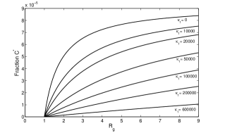
(a)

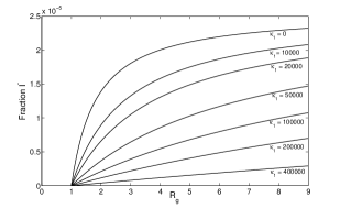
(b)

Figure 3: The equilibrium values $C^{\ast}$ (a) and $I^{\ast}$ (b) varying the reproduction number $R_{g}$ for values of $\kappa_{1}$ (with $\kappa_{2}=1.5\kappa_{1}$) from $0$ to $60\times 10^{4}$. Both $C^{\ast}$ and $I^{\ast}$ decrease as inhibition coefficients $\kappa_{1}$ and $\kappa_{2}$ increase.

Table 3 shows the equilibrium values for $\beta_{1}=7.051$ and $\beta_{2}=10.577$ (both in $years^{-1}$) resulting in $R_{g}=4$, for $\kappa_{1}=0$, $\kappa_{1}=2\times 10^{4}$, $\kappa_{1}=5\times 10^{4}$, $\kappa_{1}=10\times 10^{4}$, and $\kappa_{1}=40\times 10^{4}$ (with $\kappa_{2}=1.5\kappa_{1}$). In the absence of criminality, the coordinates of the trivial equilibrium point $P^{0}$ are $S_{1}^{0}=0.1613$, $E^{0}=0.8303$, and $S^{0}=0.0084$. The sum of all crime-related coordinates (each column) of the non-trivial equilibrium point $P^{\ast}$ is equal to $S^{0}$. When $\kappa_{1}=0$, the crime prevalence is $C^{\ast}+I^{\ast}=9.06\times 10^{-5}$.

Table 3: The equilibrium values for $\beta_{1}=7.051$ and $\beta_{2}=10.577$ (both in $years^{-1}$) resulting in $R_{g}=4$, for $\kappa_{1}=0$, $\kappa_{1}=2\times 10^{4}$, $\kappa_{1}=5\times 10^{4}$, $\kappa_{1}=10\times 10^{4}$, and $\kappa_{1}=40\times 10^{4}$ (with $\kappa_{2}=1.5\kappa_{1}$).

$\kappa_{1}$	$0$	$2\times 10^{4}$	$5\times 10^{4}$	$10\times 10^{4}$	$40\times 10^{4}$
$S^{\ast}$	$1.87\times 10^{-3}$	$4.6\times 10^{-3}$	$5.57\times 10^{-3}$	$6.72\times 10^{-3}$	$7.87\times 10^{-3}$
$L^{\ast}$	$1.42\times 10^{-4}$	$0.9\times 10^{-4}$	$0.58\times 10^{-4}$	$0.36\times 10^{-4}$	$0.11\times 10^{-4}$
$U^{\ast}$	$5.49\times 10^{-3}$	$3.47\times 10^{-3}$	$2.24\times 10^{-3}$	$1.41\times 10^{-3}$	$0.44\times 10^{-3}$
$C^{\ast}$	$7.06\times 10^{-5}$	$4.47\times 10^{-5}$	$2.89\times 10^{-5}$	$1.81\times 10^{-5}$	$0.56\times 10^{-5}$
$I^{\ast}$	$2.00\times 10^{-5}$	$1.27\times 10^{-5}$	$0.82\times 10^{-5}$	$0.51\times 10^{-5}$	$0.16\times 10^{-5}$
$F^{\ast}$	$5.55\times 10^{-4}$	$3.48\times 10^{-4}$	$2.25\times 10^{-4}$	$1.41\times 10^{-4}$	$0.44\times 10^{-4}$
$D^{\ast}$	$1.83\times 10^{-5}$	$1.16\times 10^{-5}$	$0.75\times 10^{-5}$	$0.47\times 10^{-5}$	$0.15\times 10^{-5}$
$R^{\ast}$	$2.19\times 10^{-4}$	$1.39\times 10^{-4}$	$0.90\times 10^{-4}$	$0.56\times 10^{-4}$	$0.17\times 10^{-4}$

As $\kappa_{1}$ and $\kappa_{2}$ increase, the criminals caught by police investigation ($C^{\ast}$) and the incarcerated individuals ($I^{\ast}$) decrease. The crime prevalence $C^{\ast}+I^{\ast}$, in comparison with $\kappa_{1}=0$, is reduced to $63.4\%$ ($\kappa_{1}=2\times 10^{4}$), $40.9\%$ ($\kappa_{1}=5\times 10^{4}$), $20.5\%$ ($\kappa_{1}=10\times 10^{4}$), and $7.9\%$ ($\kappa_{1}=40\times 10^{4}$). In other words, the effects of the offenders caught by police and incarceration of criminals on the naive individuals increase the dilemma to commit a crime.

Figure 4 shows the long-term (a) and short-term (b) trajectories of $C$, for $\kappa_{1}=0$, $\kappa_{1}=2\times 10^{4}$, $\kappa_{1}=5\times 10^{4}$, and $\kappa_{1}=40\times 10^{4}$ (with $\kappa_{2}=1.5\kappa_{1}$). In Figure 4(b), the curves with increasing values of $\kappa_{1}$ are from top to bottom. The dynamic trajectories are obtained by solving equation (5) with $\beta_{1}=7.235$ and $\beta_{2}=10.853$ (both in $years^{-1}$) resulting in $R_{g}=4$, and using the initial conditions given by equation (6) letting arbitrarily $f=0.001S^{0}$.

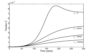
(a)

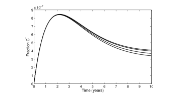
(b)

Figure 4: The long-term (a) and short-term (b) trajectories of $C$, for $\kappa_{1}=0$, $\kappa_{1}=2\times 10^{4}$, $\kappa_{1}=5\times 10^{4}$, and $\kappa_{1}=40\times 10^{4}$ (with $\kappa_{2}=1.5\kappa_{1}$). In Figure 4(b), the curves with increasing values of $\kappa_{1}$ are from top to bottom.

From Figure 4(b), the short-term (zoom near $t=0$) trajectories of $C$ showed a similar increasing phase in the first wave for all values of $\kappa_{1}$ and $\kappa_{2}$, with the curves separating after approximately $2$ $years$. The reason behind this behavior is the fact that $R_{g}$ is the same and does not depend on $\kappa_{1}$ and $\kappa_{2}$. (We recall that $R_{0}$ in epidemiology measures how fast the infection spreads out initially, while the effects of $Q$ appear later on the long-term epidemic.)

In Appendix A.1, we showed that the fraction of crime-susceptible individuals at the steady-state $\chi^{-1}$ is given by equation (A.18) for $\rho_{1}=0$. However, we supposed that $\chi^{-1}$ is given by equation (A.19) for $\rho_{1}>0$. Indeed, the asymptotic value $S^{\ast}/S^{0}$, where $S^{\ast}=\lim_{t\rightarrow\infty}S$, calculated from the dynamic trajectories $S$ (Figure 4(a) showed only the dynamic trajectories of $C$) are equal to $(1-Q)/R_{0}$ given by equation (A.19). Therefore, we have two thresholds $R_{g}=R_{0}+Q$ and $\chi^{-1}=(1-Q)/R_{0}$.

The justice system can handle the crime inhibition coefficients $\kappa_{1}$ and $\kappa_{2}$ to avoid crime practice by naive individuals. For instance, the effective police investigation and efficient court trial spread by media, and the use of handcuffs, coercive conduction, pre-trial detention, and incarceration after sentence confirmed by a lower federal court (second instance) could increase $\kappa_{1}$ and $\kappa_{2}$.

3.2 Prisoner’s dilemma – Adhere or not to the whistleblowing program

Let us consider a systemic (or epidemic) corruption in a country characterized by the crime reproduction number $R_{g}=4$ ($\beta_{1}=7.051$ and $\beta_{2}=10.577$, both in $years^{-1}$), and by the crime inhibition $\kappa_{1}=5\times 10^{4}$ and $\kappa_{2}=7.5\times 10^{4}$. This case-study corresponds to curves labeled $\kappa_{1}=50000$ in Figures 3 and 4(a), with values $C^{\ast}=3.11\times 10^{-5}$ and $I^{\ast}=0.86\times 10^{-5}$ from Table 3. We assess the effectiveness of the whistleblowing program to increase the justice system ($C^{\ast}$ and $I^{\ast}$) by varying $\varepsilon_{1}$ and $\varepsilon_{2}$ (rewards offered to the law offenders to participate in the plea bargain).

Figure 5 shows the equilibrium values $U^{\ast}$ (a) and $C^{\ast}$ (b) letting $\varepsilon_{2}=0$ and varying the reproduction number $R_{g}$ for $\varepsilon_{1}$ from $0$ to $2\times 10^{4}$ $years^{-1}$. In Figure 5(b), the curve labeled $\varepsilon_{1}=0$ corresponds to the curve labeled $\kappa_{1}=50000$ in Figure 3(a). As $\varepsilon_{1}$ increases, the number of detentions of the uncaught by police investigation $C^{\ast}$ increases.

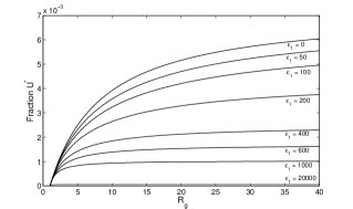
(a)

(b)

Figure 5: The equilibrium values $U^{\ast}$ (a) and $C^{\ast}$ (b) letting $\varepsilon_{2}=0$ and varying the reproduction number $R_{g}$ for $\varepsilon_{1}$ from $0$ to $2\times 10^{4}$ $years^{-1}$.

Figure 6 shows the equilibrium values $F^{\ast}$ (a) and $I^{\ast}$ (b) letting $\varepsilon_{1}=0$ and varying the reproduction number $R_{g}$ for $\varepsilon_{2}$ from $0$ to $5\times 10^{4}$ $years^{-1}$. In Figure 6(b), the curve labeled $\varepsilon_{2}=0$ corresponds to the curve labeled $\kappa_{1}=50000$ in Figure 3(b). As $\varepsilon_{2}$ increases, the number of detentions of the offenders waiting trial in freedom $I^{\ast}$ increases.

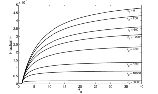
(a)

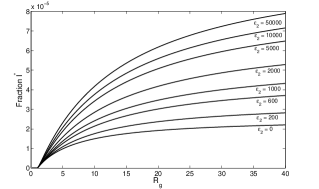
(b)

Figure 6: The equilibrium values $F^{\ast}$ (a) and $I^{\ast}$ (b) letting $\varepsilon_{1}=0$ and varying the reproduction number $R_{g}$ for $\varepsilon_{2}$ from $0$ to $5\times 10^{4}$ $years^{-1}$.

Let us illustrate the simultaneous variation of $\varepsilon_{1}$ and $\varepsilon_{2}$. Letting $\varepsilon_{2}=z_{\varepsilon}\varepsilon_{1}$, with $z_{\varepsilon}=1.5$, and varying the reproduction number $R_{g}$ for $\varepsilon_{1}$ from $0$ to $20000$ $years^{-1}$, Figure 7 shows $C^{\ast}$ for small (a) and high (b) values of $\varepsilon_{1}$. The joint action enhances the effectiveness of the justice system by increasing both $C^{\ast}$ and $I^{\ast}$ (not shown).

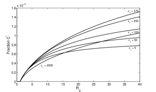
(a)

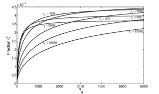
(b)

Figure 7: The equilibrium values $C^{\ast}$ (a) and $I^{\ast}$ (b) varying the crime reproduction number $R_{g}$ for $\varepsilon_{1}$ from $0$ to $20000$ $years^{-1}$, with $\varepsilon_{2}=1.5\varepsilon_{1}$.

In Figures 5 and 6, we let either $\varepsilon_{2}=0$ or $\varepsilon_{1}=0$ and varied the other parameter. When we vary $\varepsilon_{1}$ (or $\varepsilon_{2}$), individuals from class $U$ (or $F$) are transferred to $C$ (or $I$); still, the number of individuals in class $F$ (or $U$) is not affected directly by the whistleblower’s collaboration. For this reason, as $\varepsilon_{1}$ (or $\varepsilon_{2}$) increases, the number of individuals in class $U$ (or $F$) diminishes; still, the other class $F$ (or $U$) is not affected, resulting in smooth changes in the dynamic (see equation (4) for the force of law offending $\lambda$). However, the simultaneous variation of $\varepsilon_{1}$ and $\varepsilon_{2}$ illustrated in Figure 7 decreased both $U$ and $F$. Consequently, $\lambda$ decreases rapidly, and the dynamic changes qualitatively at around $\varepsilon_{1}=375$ $years^{-1}$. When $\varepsilon_{1}$ and $\varepsilon_{2}$ assume higher values but $R_{g}$ is small, the force of law offending decreases due to highly reduced numbers of individuals in $U$ and $F$, and this behavior was shown in Figure 7(a) labeled $\varepsilon_{1}=2000$. However, as $R_{g}$ increases, the numbers of individuals in $U$ and $F$ raise, and the behavior shown in Figure 7(b) followed that shown in Figures 5 and 6 – as $\varepsilon_{1}$ and $\varepsilon_{2}$ increase, $C^{\ast}$ increases.

Table 4 summarizes Figures 5-7 showing the equilibrium values varying $\varepsilon_{1}$ and $\varepsilon_{2}$. We fixed $\beta_{1}=7.051$ and $\beta_{2}=10.577$ (both in $years^{-1}$) resulting in $R_{g}=4$, and $\kappa_{1}=50000$ and $\kappa_{2}=75000$. When $\varepsilon_{1}=\varepsilon_{2}=0$, we have $U^{\ast}=2.24\times 10^{-3}$, $C^{\ast}=2.89\times 10^{-5}$, $F^{\ast}=2.25\times 10^{-4}$, and $I^{\ast}=0.82\times 10^{-5}$.

Table 4: Summary of Figures 5-7 showing the equilibrium values varying $\varepsilon_{1}$ and $\varepsilon_{2}$. The parameters $\beta_{1}=7.051$ and $\beta_{2}=10.577$ (both in $years^{-1}$) resulting in $R_{g}=4$, and $\kappa_{1}=50000$ and $\kappa_{2}=75000$ are fixed.

$\begin{array}[]{l}\varepsilon_{1}\\ \varepsilon_{2}=0\end{array}$	$\begin{array}[]{l}U^{\ast}\\ \times 10^{-3}\end{array}$	$\begin{array}[]{l}C^{\ast}\\ \times 10^{-5}\end{array}$	$\begin{array}[]{l}\varepsilon_{2}\\ \varepsilon_{1}=0\end{array}$	$\begin{array}[]{l}F^{\ast}\\ \times 10^{-4}\end{array}$	$\begin{array}[]{l}I^{\ast}\\ \times 10^{-5}\end{array}$	$\begin{array}[]{l}\varepsilon_{1}\\ \varepsilon_{2}=1.5\varepsilon_{1}\end{array}$	$\begin{array}[]{l}C^{\ast}\\ \times 10^{-5}\end{array}$	$\begin{array}[]{l}I^{\ast}\\ \times 10^{-5}\end{array}$
$0$	$2.24$	$2.89$	$0$	$2.25$	$0.82$	$0$	$2.89$	$0.82$
$100$	$1.95$	$3.08$	$600$	$1.84$	$1.03$	$50$	$2.94$	$0.88$
$400$	$1.34$	$3.50$	$2000$	$1.35$	$1.29$	$100$	$2.99$	$0.94$
$1000$	$0.78$	$3.80$	$5000$	$0.90$	$1.50$	$200$	$3.03$	$1.05$
$20000$	$0.05$	$4.07$	$50000$	$0.17$	$1.79$	$375$	$3.03$	$1.20$

As $\varepsilon_{1}$ and $\varepsilon_{2}$ increase, the criminals caught by police investigation ($C^{\ast}$) and the incarcerated individuals ($I^{\ast}$) increase, showing the effectiveness of the plea bargain. When $\varepsilon_{2}=0$, the variation in $\varepsilon_{1}$ up to $20000$ $years^{-1}$ reduced $U^{\ast}$ up to $2.23\%$ and increased $C^{\ast}$ up to $141\%$. When $\varepsilon_{1}=0$, the variation in $\varepsilon_{2}$ up to $50000$ $years^{-1}$ reduced $F^{\ast}$ up to $7.6\%$ and increased $I^{\ast}$ up to $218\%$. In other words, the dilemma to participate in the plea bargain must be increased by valuable rewards to decrease the individuals influencing positively ($U^{\ast}$ and $F^{\ast}$) and increase those impacting negatively ($C^{\ast}$ and $I^{\ast}$) to commit a crime. Notice that the overall crime is also decreased – $U^{\ast}+C^{\ast}$ up to $4\%$, and $F^{\ast}+I^{\ast}$ up to $15\%$.

The backward bifurcation occurs depending on the non-linear collaborator-dependent rate $\varepsilon_{1}$. In Appendix B.1.1, we showed the occurrence of backward bifurcation when $\beta_{1}=0$, $\kappa_{2}=0$, and $\rho_{1}=0$. Notice that $\beta_{1}=0$ means that new offenders not caught by police investigation remain “invisible” to the society and do not influence crime-susceptible individuals to commit a crime. Using values in Table 1, and letting $\varepsilon_{2}=0$, $\beta_{1}=0$, $\beta_{2}=18.090$ $years^{-1}$ (resulting in $R_{g}=1$), $\kappa_{1}=50000$ and $\kappa_{2}=1.5\kappa_{1}$, we have $C^{\ast}=0$ when $\varepsilon_{1}<\varepsilon_{1}^{c}$, and $C^{\ast}>0$ for $\varepsilon_{1}\geq\varepsilon_{1}^{c}$, with $\varepsilon_{1}^{c}=1311.8$ $years^{-1}$. Figure 8 shows the equilibrium values $C^{\ast}$ (a) and $I^{\ast}$ (b) near threshold $R_{g}=1$ and subthreshold $R^{c}\left(\varepsilon_{1}\right)$, for $\varepsilon_{1}$ from $0$ to $10000$ $years^{-1}$ – the backward bifurcation occurs when $\varepsilon_{1}\geq\varepsilon_{1}^{c}$. For $\varepsilon_{1}=1500$, $2000$, $3000$, and $10000$ (all $years^{-1}$), we have $R^{c}=0.984$, $0.902$, $0.772$, and $0.507$. In the backward bifurcation, the dotted curve (lower branch formed with small solutions $C_{<}^{\ast}$) assumes $C_{<}^{\ast}=0$ at $R_{g}=1$. Forward bifurcation is illustrated with $\varepsilon_{1}=500$ and $1000$ (all in $years^{-1}$).

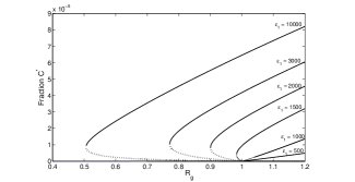
(a)

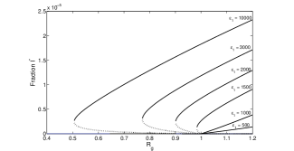
(b)

Figure 8: The equilibrium values $C^{\ast}$ (a) and $I^{\ast}$ (b) near threshold $R_{g}=1$ and subthreshold $R^{c}$, with the critical value $\varepsilon_{1}^{c}=1311.8$ $years^{-1}$.

From Figure 8, when $\varepsilon\geq\varepsilon_{1}^{c}$, we have (A) a unique $C^{\ast}>0$ for $R_{g}\geq 1$, corresponding to the non-trivial equilibrium $P^{\ast}$; (B) two equilibrium values $C_{<}^{\ast}$ (unstable equilibrium $P_{<}^{\ast}$) and $C_{>}^{\ast}$ (stable equilibrium $P_{>}^{\ast}$) for $R^{c}<R_{g}<1$; (C) at $R_{g}=R^{c}$ the two values collapse to one $C_{<}^{\ast}=C_{>}^{\ast}$; and (D) only $C^{\ast}=0$ for $R_{g}<R^{c}$, corresponding to the trivial equilibrium $P^{0}$. The backward bifurcation is characterized by the unstable branch formed by the coordinates of the equilibrium $P_{<}^{\ast}$ separating two attracting basins – letting the initial conditions at the coordinates of $P_{<}^{\ast}$, except $C(0)=C_{<}^{\ast}-\zeta$, where $\zeta>0$, the dynamic system approaches the trivial equilibrium $P^{0}$; however, for $C(0)=C_{<}^{\ast}+\zeta$, the trajectories approach to $P_{>}^{\ast}$ (see Appendix B.1.1 and Figure B.1(b)) [23]. Letting $\kappa_{1}=50000$, $\kappa_{2}=75000$, $\varepsilon_{1}=10000$ $years^{-1}$, $\varepsilon_{2}=0$, $\beta_{1}=0$, $\beta_{2}=9.711$ $years^{-1}$ (resulting in $R_{g}=0.6$), Figure 9 illustrates the role of the unstable equilibrium point $P_{<}^{\ast}$ in the dynamic system; hence, the initial conditions are

$$\left\{\begin{array}[]{l}S_{1}(0)=S_{1<}^{\ast},E(0)=E_{<}^{\ast},S(0)=S_{<}^{\ast},L(0)=L_{<}^{\ast},U(0)=U_{<}^{\ast},\\ C(0)=C_{0},F(0)=F_{<}^{\ast},I(0)=I_{<}^{\ast},D(0)=D_{<}^{\ast},R(0)=R_{<}^{\ast},\end{array}\right.$$

where the coordinates of $P_{<}^{\ast}$ are given by equation (B.2) substituting the small solution $C_{<}^{\ast}$. Letting a tiny $\zeta=0.00001C_{<}^{\ast}$, if $C_{0}=C_{<}^{\ast}-\zeta$, the attracting point is the trivial equilibrium point $P^{0}$, represented by the trajectory of $C$ in Figure 9(a). However, for $C_{0}=C_{<}^{\ast}+\zeta$, the attracting point is the non-trivial equilibrium point $P_{>}^{\ast}$, represented by the trajectory of $C$ in Figure 9(b).

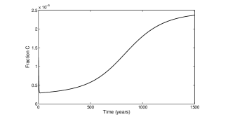
(a)

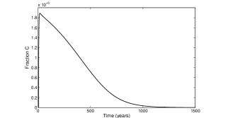
(b)

Figure 9: Illustration of two attracting basins. If $C_{0}=C_{<}^{\ast}-\zeta$, the attracting point is the trivial equilibrium point $P^{0}$ (a), while for $C_{0}=C_{<}^{\ast}+\zeta$, the attracting point is the non-trivial equilibrium point $P_{>}^{\ast}$ (b), with $\zeta=0.00001C_{<}^{\ast}$.

The plea bargain plays an essential role in criminality. The whistleblowing program benefits the justice system by helping both police investigations and court trials. Additionally, suppose that efficient measures adopted by the justice system decreased the crime reproduction number $R_{g}$ lower than one. In the absence of, or in a weak whistleblowing program ($\varepsilon<\varepsilon_{1}^{c}$), no criminals are caught ($C^{\ast}=0$). However, in an enhanced whistleblowing program, more offenders will be arrested if a critical number of criminals are convinced to collaborate with the justice system. This case can portray the imprisonments of corruptors at the highest top of the hierarchy.

4 Discussion

We developed a simplified model to describe criminality, a highly complex social phenomenon. The preceding criminality results are compared with the Covid-19 pandemic controlling efforts. The reason behind it is the common aspects of the systemic white-collar crime faced by the “car wash operation” and the Covid-19 epidemic in Brazil.

The first characteristic is the invisible agent. The struggle against corruption targets ‘invisible enemies’ that deviate budgets from education, healthcare, etc. – “they are often difficult to discover, to prove, and to punish. Such crimes are usually committed in secret, by powerful people, and with some degree of sophistication” [14]. Like other coronaviruses, SARS-CoV-2 has four structural proteins, known as the S (spike), E (envelope), M (membrane), and N (nucleocapsid) proteins; the N protein holds the RNA genome, and the S, E, and M proteins together create the viral envelope. The diameter of SARS-CoV-2 virion is 50-200 nanometers (from $5.0\times 10^{-5}$ to $20.0\times 10^{-5}$ $mm$) [6], and the image at the atomic level of the spike was obtained by cryogenic electron microscopy [21].

Another characteristic is novelty. The task force leading the “car wash operation” in Brazil faced a novel situation – the imprisonment of politicians and businessmen. Both federal judges and prosecutors had to learn how to proceed to face ‘powerful and invisible enemy’ hiding as untouchable individuals – “police, prosecutors, and the judiciary are often not well prepared for the investigation, prosecution, and judgment of these highly sophisticated crimes” [14]. Similarly, SARS-Cov-2 was initially confounded with the SARS-CoV-1 transmission, which resulted in many misguiding control efforts. The current Covid-19 pandemic showed utterly unknown, which demanded tremendous researchers’ efforts to understand the transmission of the virus, the efficient treatment, and effective vaccine [28].

We describe the fights against corruption in Brazil and associate them with the control mechanisms to mitigate the Covid-19 epidemic in Brazil to shed light on understanding and explaining the “car wash operation”.

4.1 Crime-prevention education

Figure 2 showed the equilibrium values corresponding to the law-offenders’ classes increasing as the crime reproduction number $R_{g}$ increases. The model allows to analyze the reduction in the criminality by varying the crime-prevention parameters $\eta$ and $q_{0}$, which affect the crime reproduction number $R_{g}$ given by equation (A.12). According to Dossetor [8], “a number of the most significant ‘crime prevention’ studies have not been done by criminal justice or criminology field, but by the early childhood and/or health fields, where crime prevention is but one of a number of effects derived from early childhood or home visiting interventions”.

The rapid spread of the Covid-19 epidemic required the implementation of quarantine and protective measures (use of face masks, sanitization of hands, and social distancing) [30], which showed effectiveness in controlling the pandemic. Further, the containment of the epidemic was reinforced by the introduction of vaccines. It is worth stressing the adherence to these control measures by the majority of the population. The quarantine, protective measures, and further mass vaccination to avoid infection can be compared to the crime-prevention parameters $\eta$ and $q_{0}$.

In the epidemiology model, higher values for the basic reproduction number $R_{0}$ imply a fast propagation of the disease, and more efforts are needed to eradicate the epidemic. For instance, the attempt to eliminate infection by a vaccine is achieved when the effective reproduction number $R_{ef}=1$; in other words, we must vaccinate at least a proportion $p=1-1/R_{0}$ (see Anderson and May [2]). In the case of Covid-19, it is necessary vaccinating at least $89.2\%$ (for $R_{0}=9.24$ [30]) of the population to eradicate the disease.

Using values for $q_{1}$, $q_{2}$, $q_{3}$, and $\mu$ given in Table 1, $\beta_{1}=7.051$ and $\beta_{2}=10.577$ (both in $years^{-1}$), the threshold $q_{0}^{th}=1.75\times 10^{-3}$ was calculated from equation (A.15) obtained letting $\left(\eta,\sigma,\gamma\right)\rightarrow\infty$ and $\rho_{1}=\rho_{2}=0$. (Notice that $R_{0}=q_{0}/q_{0}^{th}=5.7$, for $q_{0}=0.01$.) Therefore, it is necessary to crime-protecting at least $99.8\%$ of the population to eliminate the corruption. Interestingly, considering $R_{0}=7.63$, the Covid-19 epidemic’s first wave fades out when $99.4\%$ of individuals are immunized [31].

Another similarity with the epidemiological modeling is the role of the crime reproduction number $R_{g}=R_{0}+Q$. Figure 4 showed that the short-term dynamic was driven by the crime reproduction number $R_{g}$, while the inhibition parameters $\kappa_{1}$ and $\kappa_{2}$ affected the long-term dynamic. (We recall that $R_{0}$ in epidemiology measures how fast the infection spreads out initially, while the effects of $Q$ appear later on the long-term epidemic [26].)

4.2 Inhibition of the corruption by justice system arresting and sentencing law-offenders

Our model was formulated similar to the epidemiological modeling, where the infection is propagated depending on the contact between susceptible and infectious individuals – the force of infection increases proportionally to the number of infectious individuals. In the Covid-19 epidemic modeling, the asymptomatic individuals and fraction of mild Covid-19 cases are transmitting infection, while isolated severe Covid-19 patients in treatment are not transmitting infection; on the contrary, they influence people to adhere to control mechanisms. The criminal modeling follows these ideas: (1) the individuals uncaught ($U$) by police investigation and those caught by police but not condemned individuals (waiting for a court trial in freedom, $F$) influence and encourage crime-susceptible individuals to commit a crime (benefiting the products of crime); (2) however, the law offenders caught by police ($C$) and those sentenced by court trial ($I$) inhibit the spreading of criminality (the cost is being incarcerated). Therefore, the force of law offending increases proportionally to the law offenders evading the justice system but decreases inversely proportional to the efficacy of the justice system by catching and incarcerating law offenders. Hence, the force of law offending $\lambda$ given by equation (1) mimics the cost-benefit associated with the decision to participate in corruption.

When the “car wash operation” began (2014), the justice system was a vital ally to combat crime – a critical aspect to be mentioned is that offenders were imprisoned after condemnation sentences pronounced by lower justice courts (first and second instances). This interpretation of law resulted in the condemnation and further imprisonment of politicians and businessmen who committed corruption once the individual rights of corrupts were temporarily suspended. Moreover, media covered the combat against the corruption, showing the use of handcuffs, coercive conduction, and pre-trial detention of those under investigation. All these measures approved by the Supremo Tribunal Federal (STF, Supreme Court of Brazil) inhibited somehow the corruption.

Let us assess the decrease of corruption in an enhanced crime inhibiting society. When the media appropriately covers the corruption and the laws to combat white-collar crimes are enhanced, from Table 3, the crime prevalence $C^{\ast}+I^{\ast}$, when $\kappa_{1}$ increases from $0$ to $400000$, decreases up to $7.9\%$. The decrease in the corruption when the inhibition coefficients $\kappa_{1}$ and $\kappa_{2}$ increase was shown in Figure 3. From equation (A.16), the increase in the effectiveness of police investigation ($q_{1}$) and tribunal court ($q_{2}$) decreases the basic crime reproduction number $R_{0}$, decreasing the recruitment of new law offenders. Additionally, the increase in $C$ and $I$ decreases the force of law offending $\lambda$.

The Covid-19 pandemic shed light to show how an invisible enemy, the SARS-CoV-2, must be faced: individuals’ rights were suppressed not for days, but months [31]. Indeed, the quarantine associated with individual (sanitization of hands, use of face masks) and collective (social distancing) measures contributed to controlling the pandemic. Despite these control measures, hundreds of thousands of individuals died by lethal Covid-19 in Brazil. For this reason, the justice system correctly endorsed the suppression of individual rights for almost two years to face the struggle against an invisible enemy. In other words, individual rights were suppressed to result in collective welfare.

Summarizing, the lethality of Covid-19 resulted in the populational adherence to accept the control measures, which decreased the transmission of the virus. Roughly compared, the judicial measures suppressing white-collar criminal’s rights temporarily (use of handcuffs, coercive conduction, pre-trial detentions, for instance) and appropriate coverage of deleterious effects of corruption by media helped the “car wash operation” to combat the systemic corruption.

4.3 Plea bargain

We showed that the law offenders decreased when the inhibition coefficients $\kappa_{1}$ and $\kappa_{2}$ increased. However, the combat against corruption can be improved by the whistleblowing programs, which arrest and incarcerate ‘invisible’ white-collar criminals. In organized criminality, the identification of further law offenders is possible by convincing those caught by police investigation to adhere to the whistleblowing program. The collaboration of whistleblowers increases the efficiency of the justice system, not only catching corrupts but also inhibiting crime-susceptible individuals from committing a crime. Hence, the police-collaboration rate $\epsilon_{1}$ and judge-collaboration rate $\epsilon_{2}$ given by equation (2) mimic the reward associated with the decision to participate in the plea bargain.

As ‘invisible enemy’, the corrupts are identified by a pool of indirect shreds of evidence (no one signs a receipt of a bribe). Many judicial measures (use of handcuffs, coercive conduction, pre-trial detentions, for instance) must be used with parsimony to combat systemic corruption. Those suspicious corrupts are sentenced by court tribune after further investigations confirming their practice. These individuals are convinced to adhere to the whistleblowing program. How effective the whistleblowing program is implemented, higher becomes the justice system’s effectiveness measured by the increased incarceration of corrupts which inhibits the practice of corruption. From Table 4, the adoption of a plea bargain by the justice system, when $\varepsilon_{2}=0$ and $\varepsilon_{1}$ increases from $0$ to $20000$ $years^{-1}$, $U^{\ast}$ decreases up to $2.23\%$ and $C^{\ast}$ increases up to $141\%$, while when $\varepsilon_{1}=0$ and $\varepsilon_{2}$ increases from $0$ to $50000$ $years^{-1}$, $F^{\ast}$ decreases up to $7.6\%$ and $I^{\ast}$ increases up to $218\%$. Figures 5 and 6 showed that as the effectiveness of whistleblowing program increases, individuals uncaught by police investigation ($U$) and those waiting in freedom the court trial ($F$) are transferred to the classes of caught by police ($C$) and sentenced by court trial ($I$). In practice, the increased individuals in the classes $C$ and $I$ increase the inhibition of crime-susceptible individuals to participate in the corruption, while the decreasing in the classes $U$ and $F$ decreases the force of law-offending by crime-susceptible individuals.

As invisible enemy, Covid-19 is detected by symptoms, and those presenting symptoms are hospitalized and treated if the Real-Time Polymerase Chain Reaction (RT-PCR) test is positive. For this reason, the identification of the asymptomatic individuals by mass test and isolating those positively tested individuals is an efficient mechanism to control the SARS-CoV-2 transmission. At the early phase of the Covid-19 outbreak, many countries applied this mass screening to catch and isolate the asymptomatic individuals, which was not implemented in Brazil due to the lack of RT-PCR and serological tests. As many asymptomatic individuals should be isolated, the SARS-CoV-2 transmission must fade out quickly.

The initial investigations carried on by the “car wash operation” were able to catch a small number of corrupts. However, a well-functioning whistleblowing program helped the “car wash operation” to identify and investigate ‘invisible’ agents, sentencing, even so, a former president of Brazil. Roughly compared, a fraction of SARS-CoV-2 infection manifests Covid-19 symptoms, but mass tests identified asymptomatic individuals helping to control the epidemic.

As in the epidemiological modeling, the appearance of backward bifurcation due to the well-functioning whistleblowing policies showed the existence of more untouchable corrupts than usual (see Figures 8 and 9). In other words, to catch the highest hierarchy leaders in organized crime (corruption), the plea bargain must be very effective allied to a critical number of whistleblowers. In the disease transmission modeling, the appearance of backward bifurcation is an additional challenge to eradicate the infection because we must decrease the effective reproduction number below the sub-threshold $R_{ef}=R^{c}$ [23].

4.4 Remarks about “car wash operation” and Covid-19 epidemic’s control in Brazil

We showed the crucial role of crime inhibition and plea bargain in the preceding sections. The flowchart shown in Figure 1 and the crime reproduction number $R_{g}$ established that the police investigation (parameter $q_{1}$) is the foundation of the justice system. Based on these results, the court trial (parameter $q_{2}$ and time of court trial $1/\gamma$) must be efficient in sentencing criminals. In the “car wash operation” during 6 years, the efficient investigation of federal police (parameter $q_{1}$ higher) allied to further court trial (parameter $q_{2}$ higher and time of court trial $1/\gamma$ lower) convicted 165 individuals in both first and second instances, 49 individuals signed collaboration agreements, and 14 companies signed leniency agreements [3]. In comparison, the STF convicted only 4 individuals during this period [17]. Additionally, federal judge Moro convicted the first criminal after 12 months, while STF took 39 months [17]. This discrepancy can be naively explained by equation (A.16) – the crime reproduction number $R_{g}$ increases if $q_{1}$ and $q_{2}$ decrease, showing that the STF should not be productive unprovided of investigators.

It is worth stressing that, since 2018, the STF changed the jurisprudence and prohibited the incarceration of criminals after condemnation sentences pronounced by lower justice courts (first and second instances). Additionally, other justice measures were suppressed or weakened (use of handcuffs, coercive conduction, pre-trial detention, and plea bargain). To avoid condemnation, powerful and wealthy offenders caught by police investigation were defended and well-succeeded by famous lawyers’ offices by manipulating the flaws in law (court procedures, not the innocency of their customers) and coopting media to spread their point of view. Additionally, of greater gravity, one member of STF not only accepted their argument but declared the federal judge Moro suspicious based on records obtained by hackers. Moreover, citing a non-peer-reviewed chapter of a book [12], one member of STF released many confessed corrupts sentenced by lower instances’ federal judges stating that “the ‘car wash operation’ promoted unemployment and economic crisis in Brazil”.

Let us assess the increase of corruption in a society when crime control measures fail. When the media does not cover the corruption appropriately, and the laws to combat white-collar crimes are weakened, from Table 3, the crime prevalence $C^{\ast}+I^{\ast}$, in comparison with $\kappa_{1}=40\times 10^{4}$, is increased to $1258\%$ ($\kappa_{1}=0$), $797\%$ ($\kappa_{1}=2\times 10^{4}$), $515\%$ ($\kappa_{1}=5\times 10^{4}$), and $322\%$ ($\kappa_{1}=10\times 10^{4}$). On the other hand, from Table 4, the relaxation of the plea bargain by the justice system, when $\varepsilon_{2}=0$ and $\varepsilon_{1}$ is decreased from $20000$ $years^{-1}$ to $0$, $U^{\ast}$ is increased up to $4480\%$ and $C^{\ast}$ is decreased up to $141\%$, while when $\varepsilon_{1}=0$ and $\varepsilon_{2}$ is decreased from $50000$ $years^{-1}$ to $0$, $F^{\ast}$ is increased up to $1324\%$ and $I^{\ast}$ is decreased up to $218\%$. The overall effect is the encouragement of organized crime by increasing both $R_{g}$ and $\lambda$.

Unfortunately, we have a parallel with the Covid-19 epidemic control in Brazil. The hugely increased number of deaths due to the Covid-19 in Brazil may have several explanations – the spread of fake news (for instance, the broad use of non-scientifically proved treatments such as chloroquine, hydroxychloroquine, and ivermectin) [20], the opposition to vaccination, and depreciating the public health-threatening by opposing to the quarantine under economic argumentation (long-lasting closure of their business will affect the economy and increase unemployment). The continuous and insistently propagation of the use of non-efficient drugs as early treatment (encouraging anti-quarantine movement and non-use of individual and collective protections by a relatively significant proportion of the population), resulted in a delay in the mass immunization. As a consequence, a more virulent mutation of SARS-CoV-2 appeared [31].

Corruption does not kill as Covid-19 in a short period; still, the question is: how many and how long will the corruption practiced by the “invisible enemy” deviating national budgets result in deaths? The pandemic will last for some years, but corruption influences generations. It is worth stressing that Covid-19 fatalities increased in Brazil due to the deviation of resources allocated to the public healthcare system by politicians and businessmen. How many people died due to the lack of ICUs, healthcare workers, and vaccines? The harmful effects of systemic corruption are observed in several areas of society, for instance, the healthcare system, public education, and security.

Linking Covid-19 and corruption, we summarize that the federal authorities of Brazil opposed effective combat against an invisible enemy, letting them as a secondary public health threat. Similarly, the STF relaxed laws to fight against “secret organized” corruption. As pointed out, the plea bargain programs are not viable in weak institution environments, where protection is imperfect and court precision is low [5]. Additionally, the changes of jurisprudence by STF will signal to the Legislative (Congress) and the Executive to weaken laws to combat criminality.

The model developed to describe criminality was applied to corruption. However, this model considering crime-susceptible’s and prisoner’s dilemmas can also be used to organized crime. The justice system’s effectiveness can enhance both dilemmas to discourage the entrance into organized crime and offer rewards to disestablish the organization (by incarceration of leaders and cutting the flow of money).

5 Conclusions

We developed a deterministic model to describe organized crime considering dilemmas related to crime commitment and adherence to plea bargain. The model was applied to describe the “car wash operation” against corruption in Brazil. To better understand the rise and fall of the “car wash operation”, we compared the combat to corruption with the actions of STF and the President of Brazil to control the Covid-19 pandemic.

When “car wash operation” initiated the fight against corruption, the STF endorsed all judicial measures – (1) pre-trial detention, incarceration after sentenced by the Second Federal Court Instance (isolation of criminals by restricting individual rights), (2) uncover of hidden white-collar criminals by plea bargain (whistleblowing program), and (3) visible judicial measures (use of handcuffs and coercive conduction accompanied by appropriate media coverage). Recently, to face the Covid-19 pandemic, restrictive measures were adopted worldwide – (1) the quarantine together with restriction on the economic activities (suppressing individual rights), (2) an active search of asymptomatic and mild Covid-19 cases by mass tests (uncovering infectious individuals and isolating them), and (3) use of individual and collective protective measures appropriately propagated by the media. All these measures to control a lethal SARS-CoV-2 transmission were correctly endorsed by the STF to gain collective benefit.

The STF, however, abandoned the initial support to “car wash operation” changing the jurisprudence and restricting or even prohibiting the use of handcuffs, coercive conduction, pre-trial detention, incarceration after sentenced by the lower Federal Court, accepting fake-argumentations by lawyers, among others. It is expected that the relaxing in the combat to the corruption by justice system may increase the activities of the white-collar criminals, which misconducting Covid-19 epidemic control can shed lights. In Brazil, the President of Brazil and his staff relaxed and even opposed to the Covid-19 controlling efforts, encouraging anti-quarantine and anti-vaccine movements, use of non-scientifically proved treatments, and, also, spreading fake-news. All these actions somehow could explain the hugely increased number of deaths due to the Covid-19.

The fight against the invisible Covid-19 enemy showed that in extreme situations, extreme measures must be demanded. Indeed, our model showed that drastic measures to restrict individual rights – using handcuffs, coercive conduction, pre-trial detention, plea bargain, and other judicial actions – must be implemented with cautions to inhibit the corruption by powerful and wealthy “invisible enemies”. If the justice system is complacent with them, limiting police investigation, plea bargain, incarceration after being sentenced by the second federal court, and other harmful measures, the corruption will increase.

Conflict of interest

The authors declare there is no conflict of interest.

Appendix A The trivial equilibrium point $P^{0}$

The trivial equilibrium point $P^{0}$ of the system of equations (5), a perfect society without corruption, is given by

$$P^{0}=\left(\bar{S}_{1}=S_{1}^{0},\bar{E}=E^{0},\bar{S}=S^{0},\bar{L}=0,\bar{U}=0,\bar{C}=0,\bar{F}=0,\bar{I}=0,\bar{D}=0,\bar{R}=0\right),$$

where

$$\begin{array}[]{ccccccc}S_{1}^{0}=\frac{\mu}{\mu+\eta},&&E^{0}=\left(1-q_{0}\right)\frac{\eta}{\mu+\eta},&&\mathrm{and}&&S^{0}=q_{0}\frac{\eta}{\mu+\eta},\end{array}$$ (A.1)

with $S_{1}^{0}+E^{0}+S^{0}=1$, and $S^{0}$ is the fraction of population’s size at the risk of trespassing the law. This equilibrium point, considering $\eta\rightarrow\infty$ (well-elaborated crime-prevention policy), reduces to

$$\begin{array}[]{ccccccc}S_{1}^{0}=0,&&E^{0}=1-q_{0},&&\mathrm{and}&&S^{0}=q_{0},\end{array}$$ (A.2)

that is, the entire population is divided into two crime-protected ($E$) and crime-susceptible ($S$) classes depending only on the proportion of crime-prevention failure $q_{0}$.

The stability of $P^{0}$ is assessed by applying the next generation matrix theory considering the vector of variables $x=\left(L,U,C,F,I,R\right)$ [7]. We apply the method proposed in [24] and proved in [25]. The global stability is presented in a particular case.

A.1 The local stability

We present the existence of two thresholds – The gross reproduction number $R_{g}$ and the steady-state fraction of the crime-susceptible individuals $\chi^{-1}$ [29].

The Jacobian matrix $\bar{J}$ corresponding to the complementary vector $\bar{x}=\left(S_{1},E,S,D\right)$ evaluated at the trivial equilibrium point $P^{0}$ has negative eigen-values $\xi_{1}=-\left(\mu+\eta\right)$ and $\xi_{2}=\xi_{3}=\xi_{4}=-\mu$ (see equation (B.10) below). Therefore, the stability of the trivial equilibrium point $P^{0}$ is determined by the next generation matrix theory considering the vector of variables $x=\left(L,U,C,F,I,R\right)$.

A.1.1 The gross crime reproduction number $R_{g}$

Let us define the crime vector $f$ and the transition vector $v$ associated with the sub-system of equations (5) restricted to the variables $L$, $U$, $C$, $F$, $I$ and $R$ as

$$\begin{array}[]{lll}f^{T}=\left(\begin{array}[]{c}\frac{\beta_{1}U+\beta_{2}F}{1+\kappa_{1}C+\kappa_{2}I}S+\rho_{1}R+\rho_{2}F\\ \left(1-q_{1}\right)\sigma L\\ q_{1}\sigma L+\left(\varepsilon_{10}+\varepsilon_{1}D\right)C\\ \left(1-q_{2}-q_{3}\right)\gamma C\\ q_{2}\gamma C+\left(\varepsilon_{20}+\varepsilon_{2}D\right)F\\ \theta I\end{array}\right)&\mathrm{and}&v^{T}=\left(\begin{array}[]{c}\left(\mu+\sigma\right)L\\ \left(\mu+\varepsilon_{10}+\varepsilon_{1}D\right)U\\ \left(\mu+\gamma\right)C\\ \left(\mu+\rho_{2}+\varepsilon_{20}+\varepsilon_{2}D\right)F\\ \left(\mu+\theta\right)I\\ \left(\mu+\rho_{1}\right)R\end{array}\right),\end{array}$$ (A.3)

where $T$ stands for transposition of a matrix.

The derivatives of $f$ and $v$ with respect to $\left(L,U,C,F,I,R\right)$ evaluated at the trivial equilibrium point are denoted by the matrices $F$ and $V$, where $F$ is

$$F=\left(\begin{array}[]{cccccc}0&\beta_{1}S^{0}&0&\beta_{2}S^{0}+\rho_{2}&0&\rho_{1}\\ \left(1-q_{1}\right)\sigma&0&0&0&0&0\\ q_{1}\sigma&\varepsilon_{10}&0&0&0&0\\ 0&0&\left(1-q_{2}-q_{3}\right)\gamma&0&0&0\\ 0&0&q_{2}\gamma&\varepsilon_{20}&0&0\\ 0&0&0&0&\theta&0\end{array}\right),$$ (A.4)

and $V$ is

$$V=\left(\begin{array}[]{cccccc}\mu+\sigma&0&0&0&0&0\\ 0&\mu+\varepsilon_{10}&0&0&0&0\\ 0&0&\mu+\gamma&0&0&0\\ 0&0&0&\mu+\rho_{2}+\varepsilon_{20}&0&0\\ 0&0&0&0&\mu+\theta&0\\ 0&0&0&0&0&\mu+\rho_{1}\end{array}\right).$$ (A.5)

The next generation matrix, denoted by $FV^{-1}$, is given by

$$FV^{-1}=\left(\begin{array}[]{cccccc}0&\frac{\beta_{1}S^{0}}{\mu+\varepsilon_{10}}&0&\frac{\beta_{2}S^{0}+\rho_{2}}{\mu+\rho_{2}+\varepsilon_{20}}&0&\frac{\rho_{1}}{\mu+\rho_{1}}\\ \frac{\left(1-q_{1}\right)\sigma}{\mu+\sigma}&0&0&0&0&0\\ \frac{q_{1}\sigma}{\mu+\sigma}&\frac{\varepsilon_{10}}{\mu+\varepsilon_{10}}&0&0&0&0\\ 0&0&\frac{\left(1-q_{2}-q_{3}\right)\gamma}{\mu+\gamma}&0&0&0\\ 0&0&\frac{q_{2}\gamma}{\mu+\gamma}&\frac{\varepsilon_{20}}{\mu+\rho_{2}+\varepsilon_{20}}&0&0\\ 0&0&0&0&\frac{\theta}{\mu+\theta}&0\end{array}\right),$$

with the characteristic equation corresponding to $FV^{-1}$ being given by

$$\xi^{6}-R_{01}\xi^{4}-\left(R_{02}+Q_{F}^{1}\right)\xi^{3}-\left(R_{03}+Q_{F}^{2}+Q_{R}^{1}\right)\xi^{2}-\left(Q_{R}^{2}+Q_{R}^{3}\right)\xi-Q_{R}^{4}=0,$$ (A.6)

where the basic crime reproduction number $R_{0}$ is

$$R_{0}=R_{01}+R_{02}+R_{03},$$ (A.7)

with

$$\begin{array}[]{lllllll}R_{01}=\beta_{1}^{th}\beta_{1},&&R_{02}=\beta_{2}^{th}\beta_{2},&&\mathrm{and}&&R_{03}=\beta_{3}^{th}\beta_{2},\end{array}$$ (A.8)

where $\beta_{1}^{th}$, $\beta_{2}^{th}$, and $\beta_{3}^{th}$ are the thresholds of parameters $\beta_{1}$ and $\beta_{2}$ given by

$$\left\{\begin{array}[]{lll}\beta_{1}^{th}&=&\displaystyle\frac{\sigma}{\mu+\sigma}\left(1-q_{1}\right)\frac{S^{0}}{\mu+\varepsilon_{10}}\\ \beta_{2}^{th}&=&\displaystyle\frac{\sigma}{\mu+\sigma}q_{1}\frac{\gamma}{\mu+\gamma}\left(1-q_{2}-q_{3}\right)\frac{S^{0}}{\mu+\rho_{2}+\varepsilon_{20}}\\ \beta_{3}^{th}&=&\displaystyle\frac{\sigma}{\mu+\sigma}\left(1-q_{1}\right)\frac{\varepsilon_{10}}{\mu+\varepsilon_{10}}\frac{\gamma}{\mu+\gamma}\left(1-q_{2}-q_{3}\right)\frac{S^{0}}{\mu+\rho_{2}+\varepsilon_{20}};\end{array}\right.$$ (A.9)

and the additional crime reproduction number $Q$ is

$$Q=Q_{F}^{1}+Q_{F}^{2}+Q_{R}^{1}+Q_{R}^{2}+Q_{R}^{3}+Q_{R}^{4},$$ (A.10)

with

$$\left\{\begin{array}[]{lll}Q_{F}^{1}&=&\displaystyle\frac{\rho_{2}}{\mu+\rho_{2}+\varepsilon_{20}}\frac{\sigma}{\mu+\sigma}q_{1}\frac{\gamma}{\mu+\gamma}\left(1-q_{2}-q_{3}\right)\\ Q_{F}^{2}&=&\displaystyle\frac{\rho_{2}}{\mu+\rho_{2}+\varepsilon_{20}}\frac{\sigma}{\mu+\sigma}\left(1-q_{1}\right)\frac{\varepsilon_{10}}{\mu+\varepsilon_{10}}\frac{\gamma}{\mu+\gamma}\left(1-q_{2}-q_{3}\right)\\ Q_{R}^{1}&=&\displaystyle\frac{\rho_{1}}{\mu+\rho_{1}}\frac{\sigma}{\mu+\sigma}q_{1}\frac{\gamma}{\mu+\gamma}q_{2}\frac{\theta}{\mu+\theta}\\ Q_{R}^{2}&=&\displaystyle\frac{\rho_{1}}{\mu+\rho_{1}}\frac{\sigma}{\mu+\sigma}q_{1}\frac{\gamma}{\mu+\gamma}\left(1-q_{2}-q_{3}\right)\frac{\varepsilon_{20}}{\mu+\rho_{2}+\varepsilon_{20}}\frac{\theta}{\mu+\theta}\\ Q_{R}^{3}&=&\displaystyle\frac{\rho_{1}}{\mu+\rho_{1}}\frac{\sigma}{\mu+\sigma}\left(1-q_{1}\right)\frac{\varepsilon_{10}}{\mu+\varepsilon_{10}}\frac{\gamma}{\mu+\gamma}q_{2}\frac{\theta}{\mu+\theta}\\ Q_{R}^{4}&=&\displaystyle\frac{\rho_{1}}{\mu+\rho_{1}}\frac{\sigma}{\mu+\sigma}\left(1-q_{1}\right)\frac{\varepsilon_{10}}{\mu+\varepsilon_{10}}\frac{\gamma}{\mu+\gamma}\left(1-q_{2}-q_{3}\right)\frac{\varepsilon_{20}}{\mu+\rho_{2}+\varepsilon_{20}}\frac{\theta}{\mu+\theta}.\end{array}\right.$$ (A.11)

We interpret below $R_{0i}$, $i=1,2,3$, and $Q_{j}^{i}$, $j=F,R$ and $i=1,2,3,4$.

Equation (A.6) does not have an analytical expression for the spectral radius. However, by applying the conjecture proposed in [24] and proved in [25], we concluded that the gross crime reproduction number $R_{g}$, defined by

$$R_{g}=R_{0}+Q,$$ (A.12)

is one of the thresholds [26]. $R_{0}$ is the basic crime reproduction number, and $Q$ is an additional crime reproduction number due to the crime relapse of released ($R$) and court waiting in freedom ($F$) individuals. In epidemiological modeling, $R_{0}$ dictates the beginning of the epidemic, while the effects of $Q$ appear on the long-term dynamic (see [26]). Hence, $P^{0}$ is locally asymptotically stable if $R_{g}<1$.

The partial reproduction numbers $R_{02}$ and $R_{03}$ depending on $\beta_{2}$ obey

$$\begin{array}[]{lllll}R_{02}\geq R_{03}&&\mathrm{if}&&q_{1}\geq\frac{\varepsilon_{10}}{\mu+2\varepsilon_{10}}.\end{array}$$

If $\varepsilon_{10}=0$, then $q_{1}\geq 0$ (for all values of $q_{1}$, $R_{02}\geq R_{03}$); and for $\varepsilon_{10}\rightarrow\infty$, $R_{02}\geq R_{03}$ for $q_{1}\geq 1/2$.

Notice that $Q_{j}^{i}$ given by equation (A.11), with $j=F,R$ and $i=1,2,3,4$, depends on $\left(\varepsilon_{10},\varepsilon_{20},\rho_{1},\rho_{2}\right)$. When all parameters are zero, $\left(\varepsilon_{10},\varepsilon_{20},\rho_{1},\rho_{2}\right)=0$, then $Q_{j}^{i}=0$. However, when $\left(\varepsilon_{10},\varepsilon_{20},\rho_{1},\rho_{2}\right)\rightarrow\infty$, using that

$$\begin{array}[]{lll}\lim\limits_{\left(\rho_{2},\varepsilon_{20}\right)\rightarrow\infty}\rho_{2}/\left(\mu+\rho_{2}+\varepsilon_{20}\right)=\frac{1}{2}&\mathrm{and}&\lim\limits_{\left(\rho_{2},\varepsilon_{20}\right)\rightarrow\infty}\varepsilon_{20}/\left(\mu+\rho_{2}+\varepsilon_{20}\right)=\frac{1}{2},\end{array}$$

$Q_{j}^{i}$ depend only on $q_{1}$, $q_{2}$, and $q_{3}$ resulting, from equation (A.10), in $Q=1-q_{3}<1$. Hence, we have

$$0\leq Q=Q_{F}^{1}+Q_{F}^{2}+Q_{R}^{1}+Q_{R}^{2}+Q_{R}^{3}+Q_{R}^{4}<1$$ (A.13)

when all parameters vary from $0$ to $\infty$.

Let us analyze particular cases for the basic crime reproduction number $R_{0}$ and additional crime reproduction number $Q$. We assume the absence of self-whistleblowers, that is, $\varepsilon_{10}=0$ and $\varepsilon_{20}=0$.

1. $\sigma\rightarrow\infty$, that is, the cover-up period is zero – in this case, $\sigma/\left(\mu+\sigma\right)\rightarrow 1$ and $R_{g}=R_{0}+Q$, with

   $$\left\{\begin{array}[]{lll}R_{0}&=&\displaystyle\left(1-q_{1}\right)\frac{\beta_{1}S^{0}}{\mu}+q_{1}\frac{\gamma}{\mu+\gamma}\left(1-q_{2}-q_{3}\right)\frac{\beta_{2}S^{0}}{\mu+\rho_{2}}\\ Q&=&\displaystyle\frac{\rho_{2}}{\mu+\rho_{2}}q_{1}\frac{\gamma}{\mu+\gamma}\left(1-q_{2}-q_{3}\right)+\frac{\rho_{1}}{\mu+\rho_{1}}q_{1}\frac{\gamma}{\mu+\gamma}q_{2}\frac{\theta}{\mu+\theta}.\end{array}\right.$$

2. $\sigma\rightarrow\infty$ plus $\gamma\rightarrow\infty$, that is, the court trial period is zero – in this case, $\sigma/\left(\mu+\sigma\right)\rightarrow 1$ and $\gamma/\left(\mu+\gamma\right)\rightarrow 1$, and $R_{g}=R_{0}+Q$, with

   $$\left\{\begin{array}[]{lll}R_{0}&=&\displaystyle\left(1-q_{1}\right)\frac{\beta_{1}S^{0}}{\mu}+q_{1}\left(1-q_{2}-q_{3}\right)\frac{\beta_{2}S^{0}}{\mu+\rho_{2}}\\ Q&=&\displaystyle\frac{\rho_{2}}{\mu+\rho_{2}}q_{1}\left(1-q_{2}-q_{3}\right)+\frac{\rho_{1}}{\mu+\rho_{1}}q_{1}q_{2}\frac{\theta}{\mu+\theta}.\end{array}\right.$$

3. Besides $\sigma\rightarrow\infty$ and $\gamma\rightarrow\infty$, letting $\rho_{1}=0$ and $\rho_{2}=0$ – in this case, $Q=0$ and

   $$R_{g}=R_{0}=\displaystyle\left(1-q_{1}\right)\frac{\beta_{1}S^{0}}{\mu}+q_{1}\left(1-q_{2}-q_{3}\right)\frac{\beta_{2}S^{0}}{\mu}.$$ (A.14)

   Using $S^{0}=q_{0}$ from equation (A.2), whenever $q_{0}^{th}<q_{0}$, where $q_{0}^{th}$ is the threshold of $q_{0}$ (obtained imposing $R_{0}=1$) given by

   $$q_{0}^{th}=\displaystyle\frac{\mu}{\left(1-q_{1}\right)\beta_{1}+q_{1}\left(1-q_{2}-q_{3}\right)\beta_{2}},$$ (A.15)

   we have $R_{0}<1$, resulting in the stability of the trivial equilibrium point $P^{0}$.

To understand better the role of the fractions $q_{1}$, $q_{2}$,and $q_{3}$ in equation (A.14), let us consider $\beta_{1}=\beta_{2}=\beta$, resulting in

$$R_{g}=R_{0}=\displaystyle\left[1-q_{1}\left(q_{2}+q_{3}\right)\right]\frac{\beta S^{0}}{\mu}.$$ (A.16)

The basic crime reproduction number $R_{0}$ assumes the highest value when $q_{1}=0$ (the police investigation is completely inhibited or absent); however, for $q_{1}>0$, $R_{0}$ decreases proportionally to the increase in the incerceration by the court trial ($q_{2}$) and/or the participation of individuals caught by the police investigation in the whistleblowing program ($q_{3}$). It is worth stressing that the police innvestigation ($q_{1}$) is crucial to inhibit criminal activities.

A.1.2 The fraction of susceptible individuals $\chi^{-1}$

To calculate the second threshold, we consider a particular case, letting $\rho_{1}=0$. In this case, we remove $R$ and, using $x=\left(L,U,C,F,I\right)$, we construct the vectors $f$ and $v$ as

$$\begin{array}[]{lll}f^{T}=\left(\begin{array}[]{c}\frac{\beta_{0}+\beta_{1}U+\beta_{2}F}{1+\kappa_{1}C+\kappa_{2}I}S\\ 0\\ \varepsilon_{1}DC\\ 0\\ \varepsilon_{2}DF\end{array}\right)&\mathrm{and}&v^{T}=\left(\begin{array}[]{c}\rho_{1}R-\rho_{2}F-\left(\mu+\sigma\right)L\\ -\left(1-q_{1}\right)\sigma L+\left(\mu+\varepsilon_{10}+\varepsilon_{1}D\right)U\\ -q_{1}\sigma L-\varepsilon_{10}U+\left(\mu+\gamma\right)C\\ -\left(1-q_{2}-q_{3}\right)\gamma C+\left(\mu+\rho_{2}+\varepsilon_{20}+\varepsilon_{2}D\right)F\\ -q_{2}\gamma C-\varepsilon_{20}F+\left(\mu+\theta\right)I\end{array}\right),\end{array}$$

and the corresponding matrices $F$ and $V$ are

$$F=\left(\begin{array}[]{ccccc}0&\beta_{1}S^{0}&0&\beta_{2}S^{0}&0\\ 0&0&0&0&0\\ 0&0&0&0&0\\ 0&0&0&0&0\\ 0&0&0&0&0\end{array}\right)$$

and

$$V=\left(\begin{array}[]{ccccc}\mu+\sigma&0&0&-\rho_{2}&0\\ -\left(1-q_{1}\right)\sigma&\mu+\varepsilon_{10}&0&0&0\\ -q_{1}\sigma&-\varepsilon_{10}&\mu+\gamma&0&0\\ 0&0&-\left(1-q_{2}-q_{3}\right)\gamma&\mu+\rho_{2}+\varepsilon_{20}&0\\ 0&0&-q_{2}\gamma&-\varepsilon_{20}&\mu+\theta\end{array}\right).$$

The next generation matrix $FV^{-1}$ is given by

$$FV^{-1}=\left(\begin{array}[]{ccccc}\frac{R_{01}+R_{02}+R_{03}}{1-\left(Q_{F}^{1}+Q_{F}^{2}\right)}&A&B&C&0\\ 0&0&0&0&0\\ 0&0&0&0&0\\ 0&0&0&0&0\\ 0&0&0&0&0\end{array}\right),$$

where $A$, $B$, and $C$ are omitted ($V^{-1}$ is obtained after a tedious calculation), and the corresponding characteristic equation is given by

$$\xi^{5}-\frac{R_{01}+R_{02}+R_{03}}{1-\left(Q_{F}^{1}+Q_{F}^{2}\right)}\xi^{4}=0,$$ (A.17)

where $R_{01}$, $R_{02}$, $R_{03}$, $Q_{F}^{1}$, and $Q_{F}^{2}$ are given by equations (A.8) and (A.11). Defining the second threshold as

$$\chi=\frac{R_{01}+R_{02}+R_{03}}{1-\left(Q_{F}^{1}+Q_{F}^{2}\right)},$$

$P^{0}$ is locally asymptotically stable if $\chi<1$.

Notice that $\chi\neq 1/R_{g}$, thus the second threshold is the multiplicative inverse of the fraction of susceptible individuals given by

$$\chi^{-1}=\frac{S^{\ast}}{S^{0}}=\frac{1-\left(Q_{F}^{1}+Q_{F}^{2}\right)}{R_{01}+R_{02}+R_{03}}=\frac{1}{R_{0}}-\frac{Q_{F}^{1}+Q_{F}^{2}}{R_{0}},$$ (A.18)

according to [24]. In the general case, $\rho_{1}>0$, the calculation of $FV^{-1}$ is tough, but it is expected that

$$\chi^{-1}=\frac{S^{\ast}}{S^{0}}=\frac{1-\left(Q_{F}^{1}+Q_{F}^{2}+Q_{R}^{1}+Q_{R}^{2}+Q_{R}^{3}+Q_{R}^{4}\right)}{R_{01}+R_{02}+R_{03}}=\frac{1}{R_{0}}-\frac{Q}{R_{0}},$$ (A.19)

with $Q<1$ according to equation (A.13).

A.2 The global stability

The global stability of $P^{0}$ follows the method proposed in [18]. Let the vector of variables be $x=\left(L,U,C,F,I,R\right)$, vectors $f$ and $v$ given by equation (A.3), and matrices $F$ and $V$ given by equations (A.4) and (A.5). The vector $g$, constructed as

$$g^{T}=\left(F-V\right)x^{T}-f^{T}+v^{T},$$

is

$$g^{T}=\left(\begin{array}[]{c}\displaystyle\left(\beta_{1}U+\beta_{2}F\right)\left(S^{0}-\frac{S}{1+\kappa_{1}C+\kappa_{2}I}\right)\\ \varepsilon_{1}DC\\ -\varepsilon_{1}DC\\ \varepsilon_{2}DF\\ -\varepsilon_{2}DF\\ 0\end{array}\right),$$

where $g^{T}\geq 0$ if $S^{0}\geq S/\left(1+\kappa_{1}C+\kappa_{2}I\right)$ and $\varepsilon_{1}=\varepsilon_{2}=0$. Notice that $S^{0}\geq S$ is always true. Hence, we show the global stability for the particular case $\varepsilon_{1}=\varepsilon_{2}=0$.

Let $v_{l}=\left(z_{1},z_{2},z_{3},z_{4},z_{5},z_{6}\right)$ be the left eigenvector satisfying the equation $v_{l}V^{-1}F=\psi v_{l}$, where $\psi=\psi\left(FV^{-1}\right)$ is the spectral radius of the characteristic equation (A.6), and

$$V^{-1}F=\left[\begin{array}[]{cccccc}0&\frac{\beta_{1}S^{0}}{\mu+\sigma}&0&\frac{\beta_{2}S^{0}+\rho_{2}}{\mu+\sigma}&0&\frac{\rho_{1}}{\mu+\sigma}\\ \frac{\left(1-q_{1}\right)\sigma}{\mu+\varepsilon_{10}}&0&0&0&0&0\\ \frac{q_{1}\sigma}{\mu+\gamma}&\frac{\varepsilon_{10}}{\mu+\gamma}&0&0&0&0\\ 0&0&\frac{\left(1-q_{2}-q_{3}\right)\gamma}{\mu+\rho_{2}+\varepsilon_{20}}&0&0&0\\ 0&0&\frac{q_{2}\gamma}{\mu+\theta}&\frac{\varepsilon_{20}}{\mu+\theta}&0&0\\ 0&0&0&0&\frac{\theta}{\mu+\rho_{1}}&0\end{array}\right].$$

We must solve the system of equations

$$\left\{\begin{array}[]{rll}\displaystyle\frac{\left(1-q_{1}\right)\sigma}{\mu+\varepsilon_{10}}z_{2}+\frac{q_{1}\sigma}{\mu+\gamma}z_{3}&=&\psi z_{1}\\ \displaystyle\frac{\beta_{1}S^{0}}{\mu+\sigma}z_{1}+\frac{\varepsilon_{10}}{\mu+\gamma}z_{3}&=&\psi z_{2}\\ \displaystyle\frac{\left(1-q_{2}-q_{3}\right)\gamma}{\mu+\rho_{2}+\varepsilon_{20}}z_{4}+\frac{q_{2}\gamma}{\mu+\theta}z_{5}&=&\psi z_{3}\\ \displaystyle\frac{\beta_{2}S^{0}+\rho_{2}}{\mu+\sigma}z_{1}+\frac{\varepsilon_{20}}{\mu+\theta}z_{5}&=&\psi z_{4}\\ \displaystyle\frac{\theta}{\mu+\rho_{1}}z_{6}&=&\psi z_{5}\\ \displaystyle\frac{\rho_{1}}{\mu+\sigma}z_{1}&=&\psi z_{6},\end{array}\right.$$

and the coordinates of the vector $v_{l}$ are given by

$$\left\{\begin{array}[]{lll}z_{1}&=&\displaystyle\psi^{2}\frac{\left(\mu+\sigma\right)\left(\mu+\rho_{1}\right)}{\theta\rho_{1}}\\ z_{2}&=&\displaystyle\frac{1}{\psi^{3}}\left\{\frac{\beta_{1}S^{0}\left(\mu+\rho_{1}\right)}{\theta\rho_{1}}\psi^{4}+\frac{\varepsilon_{10}}{\mu+\gamma}\right.\\ &&\left.\times\displaystyle\left[\frac{\left(1-q_{2}-q_{3}\right)\gamma}{\mu+\rho_{2}+\varepsilon_{20}}\left(\frac{\left(\mu+\rho_{1}\right)\left(\beta_{2}S^{0}+\rho_{2}\right)}{\theta\rho_{1}}\psi^{2}+\frac{\varepsilon_{20}}{\mu+\theta}\right)+\frac{q_{2}\gamma}{\mu+\theta}\psi\right]\right\}\\ z_{3}&=&\displaystyle\frac{1}{\psi^{2}}\left\{\frac{\left(1-q_{2}-q_{3}\right)\gamma}{\mu+\rho_{2}+\varepsilon_{20}}\left[\frac{\left(\mu+\rho_{1}\right)\left(\beta_{2}S^{0}+\rho_{2}\right)}{\theta\rho_{1}}\psi^{2}+\frac{\varepsilon_{20}}{\mu+\theta}\right]+\frac{q_{2}\gamma}{\mu+\theta}\psi\right\}\\ z_{4}&=&\displaystyle\frac{1}{\psi}\left[\frac{\left(\mu+\rho_{1}\right)\left(\beta_{2}S^{0}+\rho_{2}\right)}{\theta\rho_{1}}\psi^{2}+\frac{\varepsilon_{20}}{\mu+\theta}\right]\\ z_{5}&=&1\\ z_{6}&=&\displaystyle\psi\frac{\mu+\rho_{1}}{\theta},\end{array}\right..$$

where we used the spectral radius $\psi$ as the solution of equation (A.6).

A Lyapunov function $L_{y}$ can be constructed as $L_{y}=v_{l}V^{-1}x^{T}$, resulting in

$$\begin{array}[]{ccl}L_{y}&=&\displaystyle\frac{z_{1}}{\mu+\sigma}L+\frac{z_{2}}{\mu+\varepsilon_{10}}U+\frac{z_{3}}{\mu+\gamma}C+\frac{z_{4}}{\mu+\rho_{2}+\varepsilon_{20}}F+\frac{1}{\mu+\theta}I+\frac{z_{6}}{\mu+\rho_{1}}R,\end{array}$$

which is always positive or zero ($L_{y}\geq 0$), and

$$\begin{array}[]{ccl}\frac{d}{dt}L_{y}&=&-\displaystyle\frac{1}{\psi}\frac{z_{1}}{\mu+\sigma}\left(\beta_{1}U+\beta_{2}F\right)\left(S^{0}-\psi\frac{S}{1+\kappa_{1}C+\kappa_{2}I}\right)-\frac{1}{\psi}\left(1-\psi\right)\\ &&\times\displaystyle\left[\psi z_{1}L+z_{3}\left(\varepsilon_{10}U+C\right)+\left(\frac{\rho_{2}}{\mu+\sigma}z_{1}+\frac{\varepsilon_{20}}{\mu+\theta}\right)F+\psi I+\frac{\mu+\rho_{1}}{\theta}R\right],\end{array}$$

which is negative or zero ($dL_{y}/dt\leq 0$) only if $\psi\leq 1$, and $S^{0}\geq S/\left(1+\kappa_{1}C+\kappa_{2}I\right)$, the letter is the condition to have $g^{T}\geq 0$.

Hence, the method proposed in [18] is valid only for $\varepsilon_{1}=\varepsilon_{2}=0$, in which case $P^{0}$ is globally stable if $\psi\leq 1$, and $S^{0}\geq S/\left(1+\kappa_{1}C+\kappa_{2}I\right)$. When $\varepsilon_{1}>0$ and/or $\varepsilon_{2}>0$, $P^{0}$ is locally asymptotically stable, and two positive solutions can occur when $R_{g}<1$.

A.3 Interpreting $R_{0}$ and $Q$

To interpret $R_{0}$ and $Q$, we define the following probabilities:

1. $\displaystyle p_{\sigma}=\frac{\sigma}{\mu+\sigma}$ – Probability of surviving in the class $L$, and entering into the next class.

2. $\displaystyle p_{\gamma}=\frac{\gamma}{\mu+\gamma}$ – Probability of surviving in the class $C$, and entering into the next class.

3. $\displaystyle p_{\varepsilon_{10}}=\frac{\varepsilon_{10}}{\mu+\varepsilon_{10}}$ – Probability of surviving in the class $U$, and entering into the class $C$.

4. $\displaystyle p_{\varepsilon_{20}}=\frac{\varepsilon_{20}}{\mu+\rho_{2}+\varepsilon_{20}}$ – Probability of surviving and not relapsing in the class $F$, and entering into the class $I$.

5. $\displaystyle p_{\rho_{2}}=\frac{\rho_{2}}{\mu+\rho_{2}+\varepsilon_{20}}$ – Probability of surviving and not being incarcerated in the class $F$, and entering into the class $L$.

6. $\displaystyle p_{\rho_{1}}=\frac{\rho_{1}}{\mu+\rho_{1}}$ – Probability of surviving in the class $R$, and entering into the class $L$.

7. $\displaystyle p_{\theta}=\frac{\theta}{\mu+\theta}$ – Probability of surviving in the class $I$, and entering into the class $R$.

A.3.1 Understanding $R_{0}$

The basic crime reproduction number $R_{0}=R_{01}+R_{02}+R_{03}$, given by equation (A.7), measures the strength of the criminality outbreak (beginning of the epidemic, short-term dynamic) influencing crime-susceptible individuals. The force of law-offending $\lambda$, given by equation (1), depends on the individuals in classes $U$ and $F$. From $L$, there is a unique route to reach $U$, but two routes to reach $F$. Once in these classes, they influence crime-susceptible individuals to offend the law.

1. Reaching the class $U$ from $L$ and influencing criminality – $R_{01}$. One individual in class $L$ survives in this class with probability $p_{\sigma}$ and enters into class $U$ with probability $1-q_{1}$. During the period $1/\left(\mu+\varepsilon_{10}\right)$ staying in class $U$, he/she influences $\beta_{1}S^{0}/\left(\mu+\varepsilon_{10}\right)$ individuals to commit a crime.

2. Reaching the class $F$ from $L$ and influencing criminality.

   2.a.

   From $L$ to $C$ and reaching $F$ – $R_{02}$. One individual in class $L$ survives in this class with probability $p_{\sigma}$ and enters into class $C$ with probability $q_{1}$; he/she survives in this class with probability $p_{\gamma}$ and enters into class $F$ with probability $1-q_{2}-q_{3}$. During the period $1/\left(\mu+\rho_{2}+\varepsilon_{20}\right)$ staying in class $F$, he/she influences $\beta_{2}S^{0}/\left(\mu+\rho_{2}+\varepsilon_{20}\right)$ individuals to commit a crime.

   2.b

   From $L$ to $U$ to $C$ and reaching $F$ – $R_{03}$. One individual in class $L$ survives in this class with probability $p_{\sigma}$ and enters into class $U$ with probability $1-q_{1}$; he/she survives in this class with probability $p_{\varepsilon_{10}}$ and enters into class $C$, where survives with probability $p_{\gamma}$ and enters into class $F$ with probability $1-q_{2}-q_{3}$. During the period $1/\left(\mu+\rho_{2}+\varepsilon_{20}\right)$ staying in class $F$, he/she influences $\beta_{2}S^{0}/\left(\mu+\rho_{2}+\varepsilon_{20}\right)$ individuals to commit a crime.

Therefore, $R_{0}$ is all secondary criminal co-optations produced by one offender in a crime-free community. The basic crime reproduction number depends on the non-linear terms in equation (5).

A.3.2 Understanding $Q$

The additional crime reproduction number $Q$, given by equation (A.10), measures the strength of the criminality epidemic (long-term dynamic) influencing crime-susceptible individuals. $Q$ accounts for the additional influence on the crime-susceptible individuals by the court waiting in freedom ($F$) and released ($R$) individuals when they relapse and commit crime again. Notice that an individual in $F$ returning to class $L$ has two routes to reach $F$ again ($Q_{F}^{1}$ and $Q_{F}^{2}$). However, an individual in $R$ returning to class $L$ has four routes to reach $R$ again ($Q_{R}^{1}$, $Q_{R}^{2}$, $Q_{R}^{3}$, and $Q_{R}^{4}$).

1. Leaving and returning to the same class $F$ and influencing criminality again – $Q_{F}^{1}$ and $Q_{F}^{2}$.

   1.a.

   From $F$ to $L$ to $C$ and reaching $F$ again – $Q_{F}^{1}$. One individual in class $F$ survives in this class with probability $p_{\rho_{2}}$ and enters into class $L$, where he/she survives with probability $p_{\sigma}$ and enters into class $C$ probability $q_{1}$. He/she survives this class with probability $p_{\gamma}$ and re-enters into class $F$ with probability $1-q_{2}-q_{3}$.

   1.b.

   From $F$ to $L$ to $U$ to $C$ and reaching $F$ again – $Q_{F}^{2}$. One individual in class $F$ survives in this class with probability $p_{\rho_{2}}$ and enters into class $L$, where he/she survives with probability $p_{\sigma}$ and enters into class $U$ probability $1-q_{1}$. He/she survives this class with probability $p_{\varepsilon_{10}}$ and enters into class $C$, where he/she survives with probability $p_{\gamma}$ and re-enters into class $F$ with probability $1-q_{2}-q_{3}$.

2. Leaving and returning to the same class $R$ and influencing criminality again – $Q_{R}^{1}$, $Q_{R}^{2}$, $Q_{R}^{3}$, and $Q_{R}^{4}$.

   2.a.

   From $R$ to $L$ to $C$ to $I$ and reaching $R$ again – $Q_{R}^{1}$. One individual in class $R$ survives in this class with probability $p_{\rho_{1}}$ and enters into class $L$, where he/she survives with probability $p_{\sigma}$ and enters into class $C$ probability $q_{1}$. He/she survives this class with probability $p_{\gamma}$ and enters into class $I$ with probability $q_{2}$, where he/she survives with probability $p_{\theta}$ and re-enters into class $R$.

   2.b

   From $R$ to $L$ to $C$ to $F$ to $I$ and reaching $R$ again – $Q_{R}^{2}$. One individual in class $R$ survives in this class with probability $p_{\rho_{1}}$ and enters into class $L$, where he/she survives with probability $p_{\sigma}$ and enters into class $C$ probability $q_{1}$. He/she survives this class with probability $p_{\gamma}$ and enters into class $F$ with probability $1-q_{2}-q_{3}$, where he/she survives with probability $p_{\varepsilon_{20}}$ and enters into class $I$, from which survives with probability $p_{\theta}$ and re-enters into class $R$.

   2.c.

   From $R$ to $L$ to $U$ to $C$ to $I$ and reaching $R$ again – $Q_{R}^{3}$. One individual in class $R$ survives in this class with probability $p_{\rho_{1}}$ and enters into class $L$, where he/she survives with probability $p_{\sigma}$ and enters into class $U$ probability $1-q_{1}$. He/she survives this class with probability $p_{\varepsilon_{10}}$ and enters into class $C$, where he/she survives with probability $p_{\gamma}$ and enters into class $I$ with probability $q_{2}$, from which survives with probability $p_{\theta}$ and re-enters into class $R$.

   2.d.

   From $R$ to $L$ to $U$ to $C$ to $F$ to $I$ and reaching $R$ again – $Q_{R}^{4}$. One individual in class $R$ survives in this class with probability $p_{\rho_{1}}$ and enters into class $L$, where he/she survives with probability $p_{\sigma}$ and enters into class $U$ probability $1-q_{1}$. He/she survives this class with probability $p_{\varepsilon_{10}}$ and enters into class $C$, where he/she survives with probability $p_{\gamma}$ and enters into class $F$ with probability $1-q_{2}-q_{3}$. He/she survives this class with probability $p_{\varepsilon_{20}}$ and enters into class $I$, where he/she survives with probability $p_{\theta}$ and re-enters into class $R$.

Therefore, $Q$ is all additional criminal co-optations produced by one offender when relapsing and committing a crime again. The additional crime reproduction number depends on the linear terms in equation (5).

Appendix B The non-trivial equilibrium point $P^{\ast}$

The non-trivial equilibrium point $P^{\ast}$ of the system of equations (5), the law offenders’ imprisonment, has the coordinates given by

$$\begin{array}[]{lll}P^{\ast}&=&\left(\bar{S}_{1}=S_{1}^{0},\bar{E}=E^{0},\bar{S}=S^{\ast},\bar{L}=L^{\ast},\bar{U}=U^{\ast},\right.\\ &&\left.\bar{C}=C^{\ast},\bar{F}=F^{\ast},\bar{I}=I^{\ast},\bar{D}=D^{\ast},\bar{R}=R^{\ast}\right),\end{array}$$ (B.1)

where $S^{0}=S^{\ast}+L^{\ast}+U^{\ast}+C^{\ast}+F^{\ast}+I^{\ast}+D^{\ast}+R^{\ast}$, and $S^{0}$, $S_{1}^{0}$, and $E^{0}$ are given by equation (A.1). The coordinates of the non-trivial equilibrium point $P^{\ast}$ given by equation (B.1) are

$$\left\{\begin{array}[]{lll}S^{\ast}&=&\displaystyle\frac{S^{0}\left(1+\kappa_{1}C^{\ast}+\kappa_{2}I^{\ast}\right)}{1+\kappa_{1}C^{\ast}+\kappa_{2}I^{\ast}+\frac{\beta_{1}}{\mu}U^{\ast}+\frac{\beta_{2}}{\mu}F^{\ast}}\\ L^{\ast}&=&\displaystyle\frac{\mu+\gamma}{\mu}\times\frac{\mu+\varepsilon_{10}+\frac{\varepsilon_{1}q_{3}\gamma}{\mu}C^{\ast}}{\frac{\sigma}{\mu}\left(\mu+\varepsilon_{10}+\frac{\varepsilon_{1}q_{3}\gamma}{\mu}C^{\ast}\right)-\left(1-q_{1}\right)\sigma}C^{\ast}\\ U^{\ast}&=&\displaystyle\frac{\left(1-q_{1}\right)\sigma}{\mu+\varepsilon_{10}+\frac{\varepsilon_{1}q_{3}\gamma}{\mu}C^{\ast}}\times\frac{\mu+\gamma}{\mu}\times\frac{\mu+\varepsilon_{10}+\frac{\varepsilon_{1}q_{3}\gamma}{\mu}C^{\ast}}{\frac{\sigma}{\mu}\left(\mu+\varepsilon_{10}+\frac{\varepsilon_{1}q_{3}\gamma}{\mu}C^{\ast}\right)-\left(1-q_{1}\right)\sigma}C^{\ast}\\ F^{\ast}&=&\displaystyle\frac{\left(1-q_{2}-q_{3}\right)\gamma}{\mu+\rho_{2}+\varepsilon_{20}+\frac{\varepsilon_{2}q_{3}\gamma}{\mu}C^{\ast}}C^{\ast}\\ I^{\ast}&=&\displaystyle\frac{\left(1-q_{3}\right)\gamma}{\mu+\theta}C^{\ast}-\frac{\mu+\rho_{2}}{\mu+\theta}\times\frac{\left(1-q_{2}-q_{3}\right)\gamma}{\mu+\rho_{2}+\varepsilon_{20}+\frac{\varepsilon_{2}q_{3}\gamma}{\mu}C^{\ast}}C^{\ast}\\ D^{\ast}&=&\displaystyle\frac{q_{3}\gamma}{\mu}C^{\ast}\\ R^{\ast}&=&\displaystyle\frac{\theta}{\mu+\rho_{1}}\left[\frac{\left(1-q_{3}\right)\gamma}{\mu+\theta}C^{\ast}-\frac{\mu+\rho_{2}}{\mu+\theta}\times\frac{\left(1-q_{2}-q_{3}\right)\gamma}{\mu+\rho_{2}+\varepsilon_{20}+\frac{\varepsilon_{2}q_{3}\gamma}{\mu}C^{\ast}}C^{\ast}\right],\end{array}\right.$$ (B.2)

where $C^{\ast}$ is solution of $Pol_{5}(C)\times C=0$, with $Pol_{5}(C)$ being a $5^{th}$ degree polynomial given by

$$Pol_{5}(C)=c_{5}C^{5}+c_{4}C^{4}+c_{3}C^{3}+c_{2}C^{2}+c_{1}C+c_{0},$$ (B.3)

with the coefficients $c_{i}$, $i=0,1,\cdots,5$, being given by

$$\left\{\begin{array}[]{lll}c_{5}&=&a_{6}^{2}a_{7}^{2}a_{9}a_{10}a_{12}\left(\kappa_{1}+\kappa_{2}\frac{a_{5}}{\mu+\theta}\right)\left[1-\frac{a_{1}a_{12}}{a_{1}a_{12}-a_{4}}\left(Q_{R}^{1}+Q_{R}^{3}+Q_{R}^{2th}+Q_{R}^{4th}\right)\right]\\ c_{4}&=&B_{2}D_{3}+B_{3}D_{2}\\ c_{3}&=&B_{1}D_{3}+B_{2}D_{2}+B_{3}D_{1}-A_{2}A_{5}\\ c_{2}&=&A_{3}D_{3}+B_{1}D_{2}+B_{2}D_{1}-\left(A_{1}A_{5}+A_{2}A_{4}\right)\\ c_{1}&=&A_{3}D_{2}+B_{1}D_{1}-\left(A_{1}A_{4}+A_{2}A_{3}\right)\\ c_{0}&=&a_{1}a_{2}^{2}a_{9}a_{10}\left(a_{1}a_{12}-a_{4}\right)\left(1-R_{g}\right),\end{array}\right.$$ (B.4)

where the auxiliary parameters $A_{i}$, $i=1,\cdots,5$, are

$$\left\{\begin{array}[]{l}\begin{array}[]{ll}A_{1}=\displaystyle\frac{S^{0}}{\mu}\left[a_{2}a_{4}a_{9}\beta_{1}+a_{3}\left(a_{1}a_{12}-a_{4}\right)\beta_{2}\right],&A_{2}=\displaystyle\frac{S^{0}}{\mu}\left(a_{4}a_{7}a_{9}\beta_{1}+a_{3}a_{6}a_{12}\beta_{2}\right),\end{array}\\ \begin{array}[]{llll}A_{3}=a_{2}\left(a_{1}a_{12}-a_{4}\right),&A_{4}=a_{7}\left(a_{1}a_{12}-a_{4}\right)+a_{2}a_{6}a_{12},&\mathrm{and}&A_{5}=a_{6}a_{7}a_{12},\end{array}\end{array}\right.$$

$B_{i}$, $i=1,2,3$, are

$$\left\{\begin{array}[]{lll}B_{1}&=&\displaystyle\left(a_{1}a_{12}-a_{4}\right)\left[a_{7}+a_{2}\left(\kappa_{1}+\kappa_{2}\frac{a_{5}}{\mu+\theta}\right)+a_{3}\left(\frac{\beta_{2}}{\mu}-a_{8}\kappa_{2}\right)\right]\\ &&+\displaystyle a_{2}\left(a_{4}a_{9}\frac{\beta_{1}}{\mu}+a_{6}a_{12}\right)\\ B_{2}&=&\displaystyle a_{6}a_{12}\left[a_{7}+a_{2}\left(\kappa_{1}+\kappa_{2}\frac{a_{5}}{\mu+\theta}\right)+a_{3}\left(\frac{\beta_{2}}{\mu}-a_{8}\kappa_{2}\right)\right]\\ &&+\displaystyle\left(a_{1}a_{12}-a_{4}\right)a_{7}\left(\kappa_{1}+\kappa_{2}\frac{a_{5}}{\mu+\theta}\right)+a_{4}a_{7}a_{9}\frac{\beta_{1}}{\mu}\\ B_{3}&=&\displaystyle a_{6}a_{7}a_{12}\left(\kappa_{1}+\kappa_{2}\frac{a_{5}}{\mu+\theta}\right),\end{array}\right.$$

and $D_{i}$, $i=1,2,3$, are

$$\left\{\begin{array}[]{lll}D_{1}&=&a_{1}a_{2}a_{9}a_{10}\left(1-Q\right)\\ D_{2}&=&a_{9}a_{10}\left\{a_{1}a_{7}\left[1-\left(Q_{R}^{1}+Q_{R}^{3}+Q_{R}^{2th}+Q_{R}^{4th}\right)\right]+a_{2}a_{6}\left(1-\frac{a_{1}a_{12}}{a_{1}a_{12}-a_{4}}Q\right)\right\}\\ D_{3}&=&a_{6}a_{7}a_{9}a_{10}\left[1-\frac{a_{1}a_{12}}{a_{1}a_{12}-a_{4}}\left(Q_{R}^{1}+Q_{R}^{3}+Q_{R}^{2th}+Q_{R}^{4th}\right)\right],\end{array}\right.$$

with $Q_{R}^{2th}$ and $Q_{R}^{4th}$ being the thresholds of $Q_{R}^{2}$ and $Q_{R}^{4}$,

$$\left\{\begin{array}[]{lllll}Q_{R}^{2th}&=&\lim\limits_{\varepsilon_{20}\rightarrow\infty}Q_{R}^{2}&=&\displaystyle\frac{\rho_{1}}{\mu+\rho_{1}}\frac{\sigma}{\mu+\sigma}q_{1}\frac{\gamma}{\mu+\gamma}\left(1-q_{2}-q_{3}\right)\frac{\theta}{\mu+\theta}\\ Q_{R}^{4th}&=&\lim\limits_{\varepsilon_{20}\rightarrow\infty}Q_{R}^{4}&=&\displaystyle\frac{\rho_{1}}{\mu+\rho_{1}}\frac{\sigma}{\mu+\sigma}\left(1-q_{1}\right)\frac{\varepsilon_{10}}{\mu+\varepsilon_{10}}\frac{\gamma}{\mu+\gamma}\left(1-q_{2}-q_{3}\right)\frac{\theta}{\mu+\theta},\end{array}\right.$$

and $R_{g}$ and $Q_{R}^{i}$, $i=1,\cdots,4$, are given by equations (A.12) and (A.11). The parameters $a_{i}$, with $i=1,\cdots,14$, are

$$\left\{\begin{array}[]{l}\begin{array}[]{llll}a_{1}=\mu+\varepsilon_{10},&a_{2}=\mu+\rho_{2}+\varepsilon_{20},&a_{3}=\left(1-q_{2}-q_{3}\right)\gamma,&a_{4}=\left(1-q_{1}\right)\sigma,\end{array}\\ \begin{array}[]{lllll}a_{5}=\left(1-q_{3}\right)\gamma,&a_{6}=\displaystyle\frac{q_{3}\gamma}{\mu}\varepsilon_{1},&a_{7}=\displaystyle\frac{q_{3}\gamma}{\mu}\varepsilon_{2},&a_{8}=\displaystyle\frac{\mu+\rho_{2}}{\mu+\theta},&a_{9}=\displaystyle\frac{\mu+\gamma}{\mu},\end{array}\\ \begin{array}[]{llllll}a_{10}=\displaystyle\frac{\mu+\sigma}{\mu},&a_{11}=\displaystyle\frac{\rho_{1}}{\mu},&a_{12}=\displaystyle\frac{\sigma}{\mu},&a_{13}=\displaystyle\frac{\theta}{\mu},&\mathrm{and}&a_{14}=\displaystyle\frac{\rho_{2}}{\mu}.\end{array}\end{array}\right.$$ (B.5)

Notice that $C^{\ast}=0$ is a solution, and for $C^{\ast}>0$, $C^{\ast}$ is the positive solution(s) of $Pol_{5}(C)=0$. The denominator of $L^{\ast}$ is always positive; thus $C^{\ast}\geq 0$ is the unique restriction to be populationally feasible. Letting $\varepsilon_{2}=0$ and varying $\varepsilon_{1}$, we are transferring individuals from compartment $U$ (evading police investigation) to $C$ (caught by police), which rate is proportional to the product $U\times D$. However, the collaborator-dependent rate $\varepsilon_{2}$ transfers individuals from compartment $F$ (waiting for court trial) to $I$ (condemned and incarcerated).

B.1 Particular cases

Two particular cases of the model are presented.

B.1.1 Case 1 – $\beta_{1}=0$, $\kappa_{2}=0$, and $\rho_{1}=0$

The analytical assessment of the number of positive solutions for equation (B.3) is not an easy task. For this reason, we consider a particular case, letting $\beta_{1}=0$, $\kappa_{2}=0$ and $\rho_{1}=0$. This case removes one influencing term (by $U$), one avoiding factor (by $I$), and one relapsing to crime (by $R$). In other words, we have

$$\lambda=\displaystyle\frac{\beta_{2}F}{1+\kappa_{1}C}.$$ (B.6)

In this case, $Pol_{5}(C)$ in equation (B.3) becomes a $4^{th}$ degree polynomial $Pol_{4}(C)$ given by

$$Pol_{4}\left(C\right)=c_{5}C^{4}+c_{4}C^{3}+c_{3}C^{2}+c_{2}C+c_{1},$$ (B.7)

with

$$\left\{\begin{array}[]{lll}c_{5}&=&\varepsilon_{1}\varepsilon_{2}^{2}a_{15}^{3}\kappa_{1}\\ c_{4}&=&\varepsilon_{1}\varepsilon_{2}a_{15}^{2}\left(\frac{\beta_{2}}{\mu}a_{3}+\varepsilon_{2}a_{15}+\kappa_{1}a_{2}\right)\\ &&+\varepsilon_{2}a_{15}\kappa_{1}\left\{\varepsilon_{1}a_{2}a_{15}\left[1-\left(Q_{F}^{1}+Q_{F}^{2th}\right)\right]+\varepsilon_{2}a_{1}a_{15}\right\}\\ c_{3}&=&\varepsilon_{1}\varepsilon_{2}a_{2}a_{15}^{2}\left[1-\left(R_{02}+R_{03}^{th}\right)\right]+\varepsilon_{2}a_{1}a_{2}a_{15}\kappa_{1}\left(1-Q\right)\\ &&+\left\{\varepsilon_{1}a_{2}a_{15}\left[1-\left(Q_{F}^{1}+Q_{F}^{2th}\right)\right]+\varepsilon_{2}a_{1}a_{15}\right\}\left(\frac{\beta_{2}}{\mu}a_{3}+\varepsilon_{2}a_{15}+\kappa_{1}a_{2}\right)\\ c_{2}&=&\varepsilon_{1}a_{2}^{2}a_{15}\left[1-\left(R_{02}+Q_{F}^{1}+R_{03}^{th}+Q_{F}^{2th}\right)\right]+\varepsilon_{2}a_{1}a_{2}a_{15}\left(1-R_{0}\right)\\ &&+a_{1}a_{2}\left(\frac{\beta_{2}}{\mu}a_{3}+\varepsilon_{2}a_{15}+\kappa_{1}a_{2}\right)\left(1-Q\right)\\ c_{1}&=&a_{1}a_{2}^{2}\left(1-R_{g}\right),\end{array}\right.$$

where $Q=Q_{F}^{1}+Q_{F}^{2}$, $R_{g}=R_{0}+Q$ with $R_{0}=R_{02}+R_{03}$ (see equations (A.8) and (A.11)), $\left.a_{i}\right.^{\prime}s$ are given by equation (B.5), and $R_{03}^{th}$ and $Q_{F}^{2th}$ are the thresholds of $R_{03}$ and $Q_{F}^{2}$ given by

$$\left\{\begin{array}[]{lllll}R_{03}^{th}&=&\lim\limits_{\varepsilon_{10}\rightarrow\infty}R_{03}&=&\displaystyle\frac{\sigma}{\mu+\sigma}\left(1-q_{1}\right)\frac{\gamma}{\mu+\gamma}\left(1-q_{2}-q_{3}\right)\frac{\beta_{2}S^{0}}{\mu+\rho_{2}+\varepsilon_{20}}\\ Q_{F}^{2th}&=&\lim\limits_{\varepsilon_{10}\rightarrow\infty}Q_{F}^{2}&=&\displaystyle\frac{\sigma}{\mu+\sigma}\left(1-q_{1}\right)\frac{\gamma}{\mu+\gamma}\left(1-q_{2}-q_{3}\right)\frac{\rho_{2}}{\mu+\rho_{2}+\varepsilon_{20}},\end{array}\right.$$ (B.8)

with $R_{g}=R_{02}+R_{03}+Q_{F}^{1}+Q_{F}^{2}$. Here, we substituted $a_{6}$ and $a_{7}$ by

$$\begin{array}[]{lllll}a_{6}=a_{15}\varepsilon_{1}&\mathrm{and}&a_{7}=a_{15}\varepsilon_{2},&\mathrm{where}&a_{15}=\displaystyle\frac{q_{3}\gamma}{\mu}.\end{array}$$

The coefficients of the $Pol_{4}\left(C\right)$ are $c_{4}>0$, $c_{3}>0$, and $c_{0}<0$ if $R_{g}>1$. Hence, Descartes’ signal rule assures the existence of at least one positive solution if $R_{g}>1$. However, if $R_{g}<1$, we have $c_{0}>0$ and, depending on the signal of coefficients $c_{2}$ and $c_{1}$, zero or two positive solutions are feasible. Two positive solutions for $R_{g}<1$ occur if at $R_{g}=1$ a positive solution appears. When $R_{g}=1$, we have $c_{0}=0$, and for simplicity, let us consider $\varepsilon_{10}=\varepsilon_{20}=0$ (these parameters do not affect the qualitative behavior of the model). When $\varepsilon_{2}=0$, we have $c_{5}=0$ and $c_{4}=0$, and

$$\left\{\begin{array}[]{lll}c_{3}&=&\varepsilon_{1}a_{2}a_{15}\left(\frac{\beta_{2}}{\mu}a_{3}+\kappa_{1}a_{2}\right)\left(R_{02}-Q_{F}^{2th}\right)\\ c_{2}&=&-a_{2}^{2}a_{15}\left(R_{03}^{th}+Q_{F}^{2th}\right)\left(\varepsilon_{1}-\varepsilon_{1}^{c}\right),\end{array}\right.$$

where $\varepsilon_{1}^{c}$ is the critical value for $\varepsilon_{1}$ given by

$$\varepsilon_{1}^{c}=\frac{a_{1}a_{2}\left(\frac{\beta_{2}}{\mu}a_{3}+\kappa_{1}a_{2}\right)\left(1-Q\right)}{a_{2}^{2}a_{15}\left(R_{03}^{th}+Q_{F}^{2th}\right)},$$

and a positive $C^{\ast}=-c_{2}/c_{3}$ is possible if $c_{3}$ and $c_{2}$ have opposite signal. For simplicity, let us consider $\rho_{2}=0$, that is, $Q_{F}^{2th}=0$, resulting in $c_{3}>0$. When $\varepsilon_{1}>\varepsilon_{1}^{c}$, we have $c_{2}<0$ resulting in $C^{\ast}>0$. In this case, we have a critical value (or sub-threshold) $R^{c}<1$ such that we have only $C^{\ast}=0$ when $R_{g}\leq R^{c}$, two positive solutions $C_{<}^{\ast}$ (small) and $C_{>}^{\ast}$ (big) when $R^{c}<R_{g}<1$, and a unique positive solution $C^{\ast}>0$ if $R_{g}>1$. (At $R_{g}=1$, the small positive solution becomes zero, and assumes negative value since after.) In this case we have backward bifurcation [23], and the sub-threshold $R^{c}$ can be obtained numerically.

However, when $\varepsilon_{1}=0$, for all $\varepsilon_{2}>0$, we have $c_{5}=0$, and $c_{4}>0$, $c_{3}>0$, and $c_{2}>0$; hence, the unique feasible solution is $C^{\ast}=0$. In this case, we have the forward bifurcation [23]. Additionally, if $\beta_{2}=0$, the force of law offending is

$$\lambda=\displaystyle\frac{\beta_{1}U}{1+\kappa_{1}C+\kappa_{2}I},$$

and it is not expected the occurrence of backward bifurcation [23] for all values of $\varepsilon_{1}$ and $\varepsilon_{2}$.

Summarizing, in Figure B.1 we illustrate the forward (a) and backward (b) bifurcations, with the arrows indicating the attracting equilibrium value. In the forward bifurcation, the trivial equilibrium ($C^{\ast}=0$) is stable up to $R_{g}=1$, which becomes unstable since after and the unique non-trivial equilibrium ($C^{\ast}>0$) appears. In backward bifurcation, there arises an interval $R^{c}<R_{g}<1$ where the unstable small equilibrium ($C_{-}^{\ast}$, dotted line) separates the attraction to the stable trivial equilibrium ($C^{\ast}=0$) or to the stable big equilibrium ($C_{+}^{\ast}$, continuous line). For $R_{g}>1$, the trivial equilibrium ($C^{\ast}=0$) is unstable, and the unique non-trivial equilibrium ($C_{+}^{\ast}$) is stable, which assumes $C_{+}^{\ast}>0$ at the threshold $R_{g}=1$, but assumes $C_{+}^{\ast}=0$ at the sub-threshold $R^{c}<1$.

(a)

(b)

Figure B.1: Illustration of the forward (a) and backward (b) bifurcations, with the arrows indicating the attracting equilibrium.

B.1.2 Case 2 – $\varepsilon_{1}=\varepsilon_{2}=0$

Let us consider $\varepsilon_{1}=0$ and $\varepsilon_{2}=0$, that is, the collaboration depending on the number of whistleblowers ($D$) rates are removed. The outflows, depending on the whistleblowers, are absent from compartments $U$ ($\varepsilon_{1}=0$, evading police investigation) and $F$ ($\varepsilon_{2}=0$, postponing imprisonment by court trial), and individuals caught by police investigation ($C$) and condemned by court trial ($I$) assume the lowest values. Equation (B.3) is simplified, and $C^{\ast}$ is the positive solution of equation $P_{1}\left(C\right)\times C=0$, where the solution of the $1^{st}$ degree polynomial $P_{1}\left(C\right)$ is

$$C^{\ast}=\frac{x_{1}}{x_{2}\left(1-Q\right)}\left(R_{g}-1\right),$$ (B.9)

where $R_{g}=R_{0}+Q$ is given by equation (A.12), $R_{0}$ and $Q$ are given by equations (A.7) and (A.10), and

$$\left\{\begin{array}[]{lll}x_{1}&=&\displaystyle a_{1}a_{12}-a_{4}=\frac{q_{1}\sigma\left(\mu+\varepsilon_{10}\right)+\left(1-q_{1}\right)\sigma\varepsilon_{10}}{\mu}>0\\ x_{2}&=&\displaystyle x_{1}\left[\kappa_{1}+\kappa_{2}\left(\frac{a_{5}}{\mu+\theta}-\frac{a_{3}a_{8}}{a_{2}}\right)+\frac{\beta_{2}a_{3}}{\mu a_{2}}\right]+\frac{\beta_{1}a_{4}a_{9}}{\mu}>0.\end{array}\right.$$

Therefore, if $R_{g}\geq 1$ we have $C^{\ast}\geq 0$ since $Q<1$.

B.2 Local stability

The local stability of $P^{\ast}$ is assessed numerically by calculating the eigen-values of the Jacobian matrix evaluated at this point with coordinates given by equation (B.1). We have two eigen-values $\xi_{1}=-\left(\mu+\eta\right)$ and $\xi_{2}=-\mu$, corresponding to equations for $S_{1}$ and $E$ in the system (5), plus eight eigen-values of the Jacobian matrix $J$ given by

$$J=\left[\begin{array}[]{cccccccc}-d_{1}&0&-j_{1}&j_{4}&-j_{2}&j_{5}&0&0\\ j_{3}&-d_{2}&j_{1}&-j_{4}&\rho_{2}+j_{2}&-j_{5}&0&\rho_{1}\\ 0&\left(1-q_{1}\right)\sigma&-d_{3}&0&0&0&-\varepsilon_{1}U^{\ast}&0\\ 0&q_{1}\sigma&\varepsilon_{10}+\varepsilon_{1}D^{\ast}&-d_{4}&0&0&\varepsilon_{1}U^{\ast}&0\\ 0&0&0&\left(1-q_{2}-q_{3}\right)\gamma&-d_{5}&0&-\varepsilon_{2}F^{\ast}&0\\ 0&0&0&q_{2}\gamma&\varepsilon_{20}+\varepsilon_{2}D^{\ast}&-d_{6}&\varepsilon_{2}F^{\ast}&0\\ 0&0&0&q_{3}\gamma&0&0&-\mu&0\\ 0&0&0&0&0&\theta&0&-d_{7}\end{array}\right],$$ (B.10)

where the positive diagonal elements are

$$\left\{\begin{array}[]{l}\begin{array}[]{cccc}d_{1}=\mu+j_{3},&d_{2}=\mu+\sigma,&d_{3}=\mu+\varepsilon_{10}+\varepsilon_{1}D^{\ast},&d_{4}=\mu+\gamma,\end{array}\\ \begin{array}[]{cccc}d_{5}=\mu+\rho_{2}+\varepsilon_{20}+\varepsilon_{2}D^{\ast},&d_{6}=\mu+\theta,&\mathrm{and}&d_{7}=\mu+\rho_{1},\end{array}\end{array}\right.$$

and off diagonal elements are

$$\left\{\begin{array}[]{l}\begin{array}[]{lll}j_{1}=\displaystyle\frac{\beta_{1}S^{\ast}}{1+\kappa_{1}C^{\ast}+\kappa_{2}I^{\ast}},&j_{2}=\displaystyle\frac{\beta_{2}S^{\ast}}{1+\kappa_{1}C^{\ast}+\kappa_{2}I^{\ast}},&j_{3}=\displaystyle\frac{\beta_{1}U^{\ast}+\beta_{2}F^{\ast}}{1+\kappa_{1}C^{\ast}+\kappa_{2}I^{\ast}},\end{array}\\ \begin{array}[]{lll}j_{4}=\displaystyle-\frac{\kappa_{1}\left(\beta_{1}U^{\ast}+\beta_{2}F^{\ast}\right)S^{\ast}}{\left(1+\kappa_{1}C^{\ast}+\kappa_{2}I^{\ast}\right)^{2}},&\mathrm{and}&j_{5}=\displaystyle-\frac{\kappa_{2}\left(\beta_{1}U^{\ast}+\beta_{2}F^{\ast}\right)S^{\ast}}{\left(1+\kappa_{1}C^{\ast}+\kappa_{2}I^{\ast}\right)^{2}},\end{array}\end{array}\right.$$

with the equilibrium values given by equations (B.2) and (B.3).

If all eigen-values of $J$ are negative or have negative real part if complex, then the non-trivial equilibrium point $P^{\ast}$ is locally asymptotically stable.

References

- [1] Abrams DS (2013). The imprisoner’s dilemma: A cost-benefit approach to incarceration. Faculty Scholarship at Penn. Law 553. https://scholarship.law.upenn.edu/faculty_scholarship/553.
- [2] Anderson RM, May, RM (1991). Infectious Diseases of Human. Dynamics and Control. Oxford, New York, Tokyo: Oxford University Press: 757 p.
- [3] Bechara FR, Goldschmidt PC (2020). Lessons of operation car wash: A legal, institutional, and economic analysis. Brazil Institute/Wilson Center; Washington, DC: 140 p.
- [4] Brown DK (2004). Cost-benefit analysis in criminal law. 92 Cal. L. Rev. 323: 58 p.
- [5] Buccirossi P, Immordino G, Spagnolo G (2017). Whistleblower rewards, false reports, and corporate fraud. SITE Working Paper 42. http://hdl.handle.net/10419/204753.
- [6] Chen N, et al. (2020). Epidemiological and clinical characteristics of 99 cases of 2019 novel coronavirus pneumonia in Wuhan, China: a descriptive study. Lancet 395 (10223): 507-513. DOI:10.1016/S0140-6736(20)30211-7.
- [7] Diekmann O, Heesterbeek JAP, Roberts MG (2010). The construction of next-generation matrices for compartmental epidemic models. J. R. Soc. Interface 7: 873-885.
- [8] Dossetor K (2013). Cost-benefit analysis and its application to crime prevention and criminal justice research. AIC Reports Technical and Background Paper 42.
- [9] Easton ST, Karaivanov AK (2009). Understanding optimal criminal networks. Global Crime 10 (1-2): 41-65.
- [10] Groenendijk N (1997). A principal-agent model of corruption. Crime, Law & Social Change 27: 207-229.
- [11] Kleemans ER, Poot CJ (2008). Criminal careers in organized crime and social opportunity structure. European Journal of Criminology 5 (1): 69-98. DOI: 10.1177/1477370807084225.
- [12] Marques RM (2020). Efeitos da operação lava jato na economia brasileira. In: Gonçalves M, Ramos Filho W, Nassif MI, Melo Filho H. (Org.). Relações indecentes. . São Paulo: Tirant Lo Blanc: 92-97.
- [13] Medeiros CRO, Silveira RA (2017). Petrobrás in the webs of corruption: discursive mechanisms of the Brazilian media in Operation Car Wash coverage. Rev. Cont. Org. 31: 11-20. DOI: http://dx.doi.org/10.11606/rco.v11i31.134817.
- [14] Moro SF (2018). Preventing systemic corruption in Brazil. American Academy of Arts & Sciences. DOI:10.1162/DAED_ a_00508.
- [15] Raimundo SM, Yang HM, Massad E (2018). Contagious criminal career models showing backward bifurcations: Implications for crime control policies. Journal of Applied Mathematics 2018, Article ID 1582159, doi: https://doi.org/10.1155/2018/1582159.
- [16] Roman J, Farrell G (2002). Cost-benefit analysis for crime prevention: Opportunity costs, routine savings and crime externalities. Crime Prevention Studies 14: 53-92.
- [17] Sardinha E. (2018). STF levou 1183 dias até primeira condenação ba lava jato. Moro condenou 132 no período. Congresso em foco. In (May 30, 2028): https://congressoemfoco.uol.com.br/projeto-bula/reportagem/stf-levou-1-183-dias-ate-primeira-condenacao-na-lava-jato-moro-condenou-132-no-periodo/ (accessed on December 21, 2021).
- [18] Shuai Z, van den Driessche P (2013). Global stability of infectious disease model using Lyapunov functions. SIAM J. App. Math. 73 (4): 1513-1532.
- [19] Silva MF (1999). The political economy of corruption in Brazil. Revista de Administração de Empresas 39 (3): 26-41.
- [20] Singh B, Ryan H, Kredo T, Chaplin M, Fletcher T (2021). Chloroquine or hydroxychloroquine for prevention and treatment of COVID-19. Cochrane Database Syst Rev. 2021 Feb 12; 2(2): CD013587. DOI: 10.1002/14651858.CD013587.pub2. PMID: 33624299; PMCID: PMC8094389.
- [21] Wrapp D, et al. (2020). Cryo-EM structure of the 2019-nCoV spike in the prefusion conformation. Science 367 (6483): 1260-1263. DOI:10.1126/science.abb2507.
- [22] Yang HM (2002). Population dynamics and the epidemiological model proposed by Severo. Tema 3 (2): 227-236.
- [23] Yang HM, Raimundo SM (2010). Assessing the effects of multiple infections and long latency in the dynamics of tuberculosis. Theoretical Biology and Medical Modelling 7:41, doi: http://www.tbiomed.com/content/7/1/41.
- [24] Yang, HM (2014). The basic reproduction number obtained from Jacobian and next generation matrices – A case study of dengue transmission modelling, BioSystems 126: 52–75.
- [25] Yang, HM, Greenhalgh, D (2015). Proof of conjecture in: The basic reproduction number obtained from Jacobian and next generation matrices – A case study of dengue transmission modelling, Appl. Math. Comput. 265: 103-107.
- [26] Yang, HM (2017). The transovarial transmission in the dynamics of dengue infection: epidemiological implications and thresholds. Math. Biosc. 286: 1-15.
- [27] Yang HM, Lombardi Junior LP, Castro FFM, Yang AC (2020). Mathematical model describing Covid-19 in São Paulo State, Brazil – Evaluating isolation as control mechanism and forecasting epidemiological scenarios of release. Epidemiology and Infection 148: e155. doi: 10.1017/S0950268820001600.
- [28] Yang HM, Lombardi Junior LP, Yang AC (2021). Modeling the transmission of the new coronavirus in São Paulo State, Brazil – Assessing the epidemiological impacts of isolating young and elder persons. Math. Med. Biol.: a journ. of the IMA 38 (2):137-177. doi: 10.1093/imammb/dqaa015.
- [29] Yang HM (2021). Are the beginning and ending phases of epidemics characterized by the next generation matrices? – A case study of drug-sensitive and resistant tuberculosis model. Journal of Biological Systems 2021. https://doi.org/10.1142/S0218339021500157.
- [30] Yang HM, Lombardi Junior LP, Castro FFM, Yang AC (2021). Mathematical modeling of the transmission of SARS-CoV-2 – Evaluating the impact of isolation in São Paulo State (Brazil) and lockdown in Spain associated with protective measures on the epidemic of CoViD-19. PLoS ONE 16(6): e0252271. https://doi.org/10.1371/journal.pone.0252271.
- [31] Yang HM, Lombardi Junior LP, Castro FFM, Yang AC (2021). Evaluating the impacts of relaxation and mutation in the SARS-CoV-2 on the COVID-19 epidemic based on a mathematical model – A case study of São Paulo State (Brazil). Comput. Appl. Math. 40: 272-299. doi: https://doi.org/10.1007/s40314-021-01661-w.