BeyondPlanck XVI. Limits on large-scale polarized anomalous
microwave emission from Planck LFI and WMAP

We constrained the level of polarized anomalous microwave emission (AME) on large angular scales using Planck Low-Frequency Instrument (LFI) and WMAP polarization data within a Bayesian cosmic microwave background (CMB) analysis framework. We modeled synchrotron emission with a power-law spectral energy distribution, as well as the sum of AME and thermal dust emission through linear regression with the Planck High-Frequency Instrument (HFI) 353 GHz data. This template-based dust emission model allowed us to constrain the level of polarized AME while making minimal assumptions on its frequency dependence. We neglected cosmic microwave background fluctuations, but show through simulations that these fluctuations have a minor impact on the results. We find that the resulting AME polarization fraction confidence limit is sensitive to the polarized synchrotron spectral index prior. In addition, for prior means $\beta_{\mathrm{s}}<$ $-3.1$ we find an upper limit of $p_{\mathrm{AME}}^{\rm max}\lesssim 0.6\thinspace\%$ (95 % confidence). In contrast, for means $\beta_{\mathrm{s}}=-3.0$, we find a nominal detection of $p_{\mathrm{AME}}=2.5\pm 1.0\thinspace\%$ (95 % confidence). These data are thus not strong enough to simultaneously and robustly constrain both polarized synchrotron emission and AME, and our main result is therefore a constraint on the AME polarization fraction explicitly as a function of $\beta_{\mathrm{s}}$. Combining the current Planck and WMAP observations with measurements from high-sensitivity low-frequency experiments such as C-BASS and QUIJOTE will be critical to improve these limits further.

1 Introduction

One of the primary goals of future cosmic microwave background (CMB) missions such as CMB-S4 (Abazajian et al. 2019), Simons Observatory (Ade et al. 2019), and LiteBIRD (Sugai et al. 2020) is to detect the hypothesized signal from primordial gravitational waves, or to constrain the tensor-to-scalar ratio $r$. In order for this goal to be reached, it is essential to characterize polarized Galactic emission at the 10–100 ${\rm nK}$ level.

Two emission mechanisms dominate the polarized Galactic signal at microwave frequencies: synchrotron emission below $\sim$70 GHz and thermal dust emission above $\sim$70 GHz (e.g., Page et al. 2007; Planck Collaboration X 2016). Recent measurements from Planck have shown that the polarization fractions of these two components can reach 40 and 20 %, respectively (Planck Collaboration 2018), and their rich morphologies are connected by the Galactic magnetic field. Other emission mechanisms, such as free-free and anomalous microwave emission (AME), are important contributions to the total intensity observed in the same frequency range, but no significant polarization has been detected yet (e.g., Planck Collaboration XXV 2016), although a small free-free contribution is predicted on very small angular scales near the edges of H ii regions (Rybicki & Lightman 1985).

Anomalous microwave emission was serendipitously detected while analyzing COBE–DMR and other data sets in the 10–60 GHz range (Kogut et al. 1996; Leitch et al. 1997; de Oliveira-Costa et al. 2004). This emission is highly correlated with Galactic thermal dust morphology and has been detected within specific clouds such as the Perseus molecular cloud (Watson et al. 2005; Planck Collaboration 2016; Tibbs et al. 2010; Génova-Santos et al. 2015), $\lambda$ Orionis (Bell et al. 2019; Cepeda-Arroita et al. 2021), $\rho$ Ophiuchus (Casassus et al. 2008; Arce-Tord et al. 2020), among others (Planck Collaboration 2014), and potentially even in external galaxies (Murphy et al. 2010, 2018; Battistelli et al. 2019). However, the polarized properties of this emission is still uncertain as physical models predict varying levels of potential polarized emission (Dickinson et al. 2018).

Ignoring this component during Galactic foreground removal can have a detrimental effect on polarized CMB determination. As demonstrated by Remazeilles et al. (2016), neglecting AME models with a polarization fraction as low as $\sim$ 1 % can cause a nonnegligible bias on the measured tensor-to-scalar ratio for a wide range of proposed future missions.

The currently favored model for AME is spinning dust emission, in which the radiation is due to small, rotating dust grains with an electric or magnetic dipole moment (Draine & Lazarian 1998). The total power $P_{\nu}$ emitted at frequency $\nu$ from a single grain rotating at frequency $\omega$ = $2\pi\nu$, electric or magnetic dipole moment $\mu$, and with angle $\theta$ between its dipole moment and rotation axis is given by

$$\centering P_{\nu}=\frac{2}{3}\frac{\omega^{4}\mu^{2}\sin^{2}\theta}{c^{3}}\thinspace.\@add@centering$$ (1)

Much of the theoretical work on spinning dust emission has been devoted to predicting the distribution of grain angular velocities present in the interstellar medium, which depends on properties such as grain size and shape as well as the local environment, such as the local gas density, temperature, and ionization (Draine & Lazarian 1998; Hoang et al. 2010; Silsbee et al. 2011). These properties are poorly constrained, so theoretical predictions for the frequency spectrum of the AME are highly uncertain.

The details of this model have been combined in the SpDust2 code to produce AME spectra for varying interstellar medium conditions (Hoang et al. 2010; Silsbee et al. 2011). In Planck Collaboration IX (2016), the Commander (Eriksen et al. 2008) analysis had to combine two SpDust2 spectra in order to get a good fit to the observed AME. While theoretical studies have attributed two component AME models to emission from the cold and warm neutral media (Hoang et al. 2010; Ysard et al. 2010), a recent study found no link between the AME spectrum and the fraction of HI in the cold neutral phase (Hensley et al. 2021), casting doubt on this interpretation. In this paper, we therefore seek constraints on AME properties without imposing strong assumptions on its frequency spectrum.

The polarization of spinning dust emission depends on how efficiently they align with the local magnetic field. Hoang et al. (2013) argue that starlight polarization features in HD 197770 and HD 147933-4 could be caused by weakly aligned polycyclic aromatic hydrocarbons (PAHs), corresponding to polarization from spinning PAHs of $\lesssim 1\leavevmode\nobreak\ \%$ for frequencies $\sim$ 20 GHz. Additionally, Hoang & Lazarian (2016) calculated that iron nanoparticles can efficiently align with the Galactic magnetic field, yielding a wide range of potential polarization fractions of their microwave spinning dust emission. On the other hand, Draine & Hensley (2016) argue that quantum suppression of energy dissipation interferes with alignment of very small grains, leading to extremely small polarization fractions at microwave frequencies.

Though the spinning dust model is favored due to intensity measurements, other models have not been definitively ruled out. A theory of emission from thermal fluctuations in magnetic dust grains has been proposed by Draine & Lazarian (1999), and subsequently revisited by Draine & Hensley (2013). They identified resonance behavior that can produced peaked, AME-like spectra dependent on the magnetic properties and shapes of the grains. Predictions for polarization fractions in such resonances range from $\sim$5 to 40 %, in conflict with current best limits on AME polarization.

Theoretical predictions for the low-level polarized emission from AME are supported by most published observations. Using QUIJOTE data focused on molecular complex W43r, Génova-Santos et al. (2017) found rigid upper limits for polarized AME at 16.7, 22.7, and 40.6 GHz of 0.39, 0.52 and 0.22 % respectively. The most recent analysis of QUIJOTE data by Poidevin et al. (2019) concluded that the polarization fraction is indeed consistent with zero within the Taurus molecular cloud. This analysis found the polarization fraction of AME to be less than $4.2\thinspace\%$ ($95\thinspace\%$ confidence), assuming that all of the observed polarized emission were to come from AME. Battistelli et al. (2006) measured the total emission within the Perseus region to be polarized at $P=3.4^{+1.5}_{-1.9}\thinspace\%$ at 11 GHz ($95\thinspace\%$ confidence interval), while Planck Collaboration XXV (2016) derives a $2\thinspace\sigma$ AME polarization percentage limit of less than $1.6\thinspace\%$ within the same region. The differing results are likely due to the handling of polarized synchrotron emission, and this emphasizes the importance of synchrotron marginalization.

Macellari et al. (2011) carried out a template based cross-correlation analysis with standard foreground templates to estimate the amplitude of the Galactic components in both intensity and polarization. Correlations were determined for synchrotron, dust, and free-free emission within the WMAP 5-year maps using Haslam et al. (1982), the WMAP 94 GHz dust prediction, and the Finkbeiner (2003) H$\alpha$ maps as templates, respectively. With this method they found the polarization of both dust and free-free emission to be consistent with zero for the all-sky analysis. Concerning AME, this results in a full sky AME polarization fraction at WMAP K-band of less than $5\thinspace\%$ ($95\thinspace\%$ confidence). They also highlight dust-correlated polarization fractions at a $2\thinspace\sigma$ level within some regions of the sky within the K-band, while noting slightly negative dust polarizations (negative correlation between total intensity template and polarized emission) indicating a degeneracy between sky components.

In this work we add to earlier constraints in three key ways. Firstly, rather than investigating a specific region, we fit the level of polarized dust correlated emission using nearly the full sky. Secondly, we make no assumptions about the AME SED to avoid bias from an imperfect spectral fit. Instead, we make a strong spatial assumption, namely that AME is perfectly correlated (or anti-correlated) with thermal dust emission. Finally, we employ the Bayesian BeyondPlanck framework (BeyondPlanck 2022) to marginalize over the uncertainty in the other Galactic foregrounds and systematic effects. This approach attacks the CMB analysis problem by fitting instrumental, astrophysical and cosmological parameters all jointly within an integrated Gibbs sampling framework. The synchrotron spectral index and amplitude are independently redetermined within the current paper, to allow joint fits with the AME parameters. Technically speaking, marginalization over systematic uncertainties is implemented by analysing an ensemble of different BeyondPlanck Low-Frequency Instrument (LFI) map realizations within the sampling scheme, thereby propagating low-level uncertainties from the BeyondPlanck mapmaking procedure. This is the first example of how systematic errors may be propagated into postproduction analyses using Monte-Carlo ensembles with LFI data.

The paper is organized as follows: Section 2 describes the data used in this analysis. An overview of the sky model and sampling techniques are discussed in Sects. 3 and 4 respectively, and in Sect. 5 the results of the Gibbs sampler on the BeyondPlanck data are discussed. Concluding remarks and outlook are reported in Sect. 6. All software is made publicly available.

2 Data

Because AME is only observed between 10-60 GHz in intensity, we restrict our data selection to the 20–70 GHz frequency range. As such, our main observations are the polarization observations from the Planck LFI (Planck Collaboration II 2020) and WMAP (Bennett et al. 2013) experiments. For LFI, we adopt the BeyondPlanck 30, 44, and 70 GHz frequency sky maps (BeyondPlanck 2022), which come in the form of an ensemble of samples, each of which represents a different realization of systematic effects for the frequency channel in question. These include, but are not limited to, corrections for gain variations (Gjerløw et al. 2022), correlated noise (Ihle et al. 2022), bandpass leakage (Svalheim et al. 2022a) and far sidelobe contamination (Galloway et al. 2022). In order to properly marginalize over these uncertainties, we draw maps from an ensemble of 1000 different map realizations.

For WMAP, we include the K- (22.8 GHz), Ka- (33.0 GHz), Q- (40.6 GHz), and V-band (60.8 GHz) channels. The W-band (94 GHz) data are however excluded due to a high level of systematic residuals (Bennett et al. 2013).

In addition to these main observations, we utilize the Planck DR4 353-GHz polarization map (Planck Collaboration Int. LVII 2020a) as a tracer of polarized dust emission. We use the raw DR4 353-GHz map, with no CMB subtraction, noting that this channel is strongly dust dominated. Finally, in order to derive an estimate of the polarization fraction $p_{\rm AME}$ of AME we need an estimate of the AME intensity. For this, we adopt the Planck 2015 AME component map (Planck Collaboration X 2016), rather than the corresponding BeyondPlanck AME maps (Andersen et al. 2022), as the former was derived without strong spatial priors.

All maps are smoothed to a common angular resolution of $1^{\circ}$ FWHM Gaussian beam, and discretized using the HEALPix pixelization format (Górski et al. 2005) with a resolution parameter of ${N_{\mathrm{side}}=64}$. We adopt the cosmological convention for the definition of the Stokes $Q$ and $U$ parameters, which differs from the IAU convention only in the sign of $U$ (Górski et al. 2005). Rayleigh-Jeans brightness temperature units ($\mu{\rm K_{RJ}}$) are utilized for the entirety of this work, and full bandpass integration for both WMAP and BeyondPlanck LFI maps are taken into account during the fitting procedures.

To obtain a reliable estimate of the level of detectable polarized dust emission below 60 GHz we need to mask portions of the sky which may bias our results. At the same time, it is highly desirable to include as much of the sky as possible, to maximize our signal-to-noise ratio. We therefore choose to primarily define our primary analysis mask on the central Galactic region defined in Svalheim et al. (2022b), but additionally we mask out a few compact regions with very high $\chi^{2}$’s, including Tau-A. A total of $f_{\mathrm{sky}}=91\thinspace\%$ is included in the final analysis.

3 Sky model

3.1 Modelling considerations

In this paper, we make no assumptions regarding the AME spectral energy density (SED). Instead, we note from the Planck 2015 analysis that AME in total intensity is highly correlated with thermal dust emission (Planck Collaboration X 2016). This motivates us for now to assume that any detectable polarized AME also has the same morphology as polarized thermal dust emission as measured at 353 GHz. If the grains emitting the AME are aligned by the same magnetic field aligning those responsible for FIR polarization, and if the alignment is in the usual sense, that is the short axis parallel to the magnetic field B, then the polarization direction at AME frequencies is the same as that observed at 353 GHz (Draine & Lazarian 1998).

The polarization fraction of dust emission is a function of grain properties (alignment, shape, size), density structure, and magnetic field geometry. As shown in Planck Collaboration XII (2020) using the Planck full-sky maps, neither grain alignment nor the dust temperature drive variations in the polarization fraction over diffuse and translucent sightlines (for column densities $N_{\mathrm{H}}<8\times 10^{21}\thinspace\mathrm{cm}^{-2}$, corresponding to 98 % of the sky). The highest column densities where this conclusion breaks down lie, for the most part, within the portion of the sky which is masked out here. This conclusion is supported by Clark & Hensley (2019), who find that with H I structures alone are able to reproduce the Planck 353 GHz polarization maps at degree scales with high accuracy over most of the sky. Therefore, if the grains producing the AME and the far infrared continuum emission are aligned with the same magnetic field, we expect the polarization fraction of each to be similar. Nevertheless, it is possible that, unlike the larger grains, the alignment efficiency of nanoparticles varies substantially across the sky. In this case, the polarization fractions of the two emission mechanisms would be less correlated and AME polarization fractions in excess of those derived in this work would be permitted However, there is no strong observational evidence for this scenario and we do no consider it further in our analysis.

A known issue in AME polarization studies is the presence of polarized synchrotron emission (Planck Collaboration XXV 2016). Additionally, polarized thermal dust emission is nonnegligible even at AME frequencies. In principle, we could disentangle these distinct Galactic components by using a template for polarized synchrotron emission in a way analogous to the dust emission. However, no suitable high signal-to-noise ratio polarized synchrotron templates currently exist. As an example, one might consider using the polarized synchrotron component derived by the SMICA algorithm in Planck Collaboration IV (2018). However, this analysis explicitly assumes that the polarized thermal dust emission “vanishes at 30 GHz”, and therefore all polarized emission at 30 GHz is assigned to be exclusively synchrotron emission. This would lead to erroneously tight constraints on polarized AME emission in the current analysis. In the absence of a high signal-to-noise ratio template of polarized synchrotron emission, we adopt a simple parametric power-law model to fit the synchrotron component in each pixel, and marginalize over the free parameters.

3.2 Parametric model

We model the observed emission ${d}_{\nu,p}$ in pixel $p$ at frequency $\nu$ as the sum of the true sky signal ${s}_{\nu,\thinspace p}$ and the noise ${n}_{\nu,\thinspace p}$, given by

$${d}_{\nu,p}={s}_{\nu,p}+{n}_{\nu,p}.$$ (2)

The polarized sky signal, $s_{\nu,p}$, is usually described by three components in the microwave regime in addition to AME, namely thermal dust emission, synchrotron emission, and CMB (Planck Collaboration XXV 2016; Planck Collaboration IV 2018; Svalheim et al. 2022b). In this analysis, however, we do not include CMB because this contribution is known to be small over the frequency range and angular scales of interest (Planck Collaboration V 2020), and including unconstrained degrees of freedom typically leads to nonphysical degeneracies. Instead, we perform dedicated sensitivity tests in Sect. 5.4 by adding simulated CMB fluctuations to the existing sky maps, and show that this has a minor impact on final results. The sky model may therefore be written out in the following form,

$${s}_{\nu,p}={s}_{\mathrm{s},\nu,p}+{s}_{\mathrm{AME},\nu,p}+{s}_{\mathrm{d},\nu,p}.$$ (3)

Synchrotron emission is modeled in terms of a power-law SED with a free amplitude per Stokes parameter and pixel, $a^{Q,U}_{\mathrm{s},p}$, and a spectral index, $\beta_{\mathrm{s},p}$, per pixel, but common for $Q$ and $U$,

$$s^{Q,U}_{\mathrm{s},\nu,p}=\thinspace a^{Q,U}_{\mathrm{s},p}\thinspace\Big{(}\frac{\nu}{\nu_{\rm 0,s}}\Big{)}^{\beta_{\mathrm{s},p}}.$$ (4)

We choose a reference frequency of $\nu_{\rm 0,s}=30\thinspace{\rm GHz}$ for synchrotron emission.

For thermal dust emission, we adopt a single modified blackbody (MBB) SED,

$${s}_{\mathrm{d},\nu,p}^{Q,U}=\mathcal{T}_{\mathrm{d},p}^{Q,U}\thinspace\Big{(}\frac{\nu}{\nu_{0,\mathrm{d}}}\Big{)}^{\beta_{\rm d}+1}\thinspace\frac{e^{h\nu_{0,\mathrm{d}}/kT_{\rm d}}-1}{e^{h\nu/kT_{\rm d}}-1}.$$ (5)

where $h$ and $k$ are the Planck and Boltzmann constants, respectively; $\nu_{0,\mathrm{d}}$ is the thermal dust reference frequency, which is taken to be $353\thinspace{\rm GHz}$; ${\beta_{\rm d}}$ is the thermal dust spectral index; and $T_{\rm d}=19.6\thinspace{\rm K}$ is the dust temperature; and $\mathcal{T}_{\mathrm{d},\thinspace p}$ is the Planck 353 GHz map. We marginalize over the thermal dust spectral index using the same prior as in the main BeyondPlanck analysis ($\beta_{\rm d}=1.62\pm 0.04$; Svalheim et al. 2022b) by drawing a new value for $\beta_{\rm d}$ in each Markov chain iteration.

Finally, we assume that polarized AME is spatially perfectly correlated with polarized thermal dust emission, and we adopt the Planck DR4 353 GHz map as a spatial template for polarized AME. Allowing for a single multiplicative amplitude, $a_{\mathrm{AME},\thinspace\nu}$, for both Stokes parameters, our model reads

$$s_{\mathrm{AME},\thinspace\nu,\thinspace p}^{Q,U} =a_{\mathrm{AME},\thinspace\nu}\thinspace\mathcal{T}_{\mathrm{d},\thinspace p}^{Q,U}.$$ (6)

However, to avoid a perfect degeneracy between the spatial synchrotron template and the AME template amplitudes, a maximum of $N_{\mathrm{band}}-1$ template amplitudes can be fit. To break this degeneracy, we fix $a_{\mathrm{AME},\thinspace\nu}=0$ for the WMAP V-band (61 GHz) and LFI 70 GHz channels, where the AME-to-thermal-dust ratio in intensity is $0.033$ and $0.008$, respectively, in the Planck 2015 model (Planck Collaboration X 2016).

Collecting terms, we arrive at the final complete data model,

$$s_{\nu,p}^{Q,U}=a_{\mathrm{s},p}^{Q,U}\thinspace\left(\frac{\nu}{\nu_{\rm 0,s}}\right)^{\beta_{\mathrm{s},p}}+\mathcal{T}_{\mathrm{d},p}^{Q,U}\left(\left(\frac{\nu}{\nu_{0,\mathrm{d}}}\right)^{\beta_{\mathrm{d}}+1}\thinspace\frac{e^{h\nu_{0,\mathrm{d}}/kT_{\rm d}}\text{-}1}{e^{h\nu/kT_{\rm d}}\text{-}1}+a_{\mathrm{AME},\nu}\right)$$ (7)

In this model we fit $a_{\mathrm{s},p}^{Q,U}$ and $\beta_{\mathrm{s},p}$ per pixel, and $a_{\rm AME,\nu}$ as a single value across the sky. The synchrotron amplitude is determined independently in Stokes $Q$ and $U$, while both $\beta_{\mathrm{s}}$ and $a_{\rm AME,\nu}$ are fit jointly in $Q$ and $U$. The primary goal of the following analysis is to constrain the $a_{\rm AME,\nu}$ coefficients, and the other parameters are simply considered to be nuisance parameters that we marginalize over.

3.3 From AME template amplitudes to polarization fraction

The AME polarization fraction $p_{\mathrm{AME}}$ is defined as the ratio of the polarized ($P_{\mathrm{AME},\thinspace\nu,\thinspace p}$) and total AME intensities ($I_{\mathrm{AME},\thinspace\nu,\thinspace p}$) at each frequency $\nu$ and pixel $p$, i.e. $P_{\mathrm{AME},\thinspace\nu,\thinspace p}/I_{\mathrm{AME},\thinspace\nu,\thinspace p}$.

To translate the vector of template amplitudes, $\boldsymbol{a}_{\rm AME}$, to an AME polarization fraction, $p_{\rm AME,\thinspace\nu}$, we use Eq. (6) to associate polarized AME with polarized thermal dust emission,

$$P_{\mathrm{AME},\thinspace\nu,\thinspace p}=a_{\mathrm{AME},\thinspace\nu}\sqrt{{\mathcal{T}_{\mathrm{d},\thinspace p}^{Q}}^{2}+{\mathcal{T}_{\mathrm{d},\thinspace p}^{U}}^{2}}=a_{\mathrm{AME},\thinspace\nu}\leavevmode\nobreak\ P_{353,p}.$$ (8)

Following the results from Planck 2015, we can describe $I_{\mathrm{AME},\thinspace\nu,\thinspace p}$ as the product of the frequency dependence $f_{\mathrm{AME}}(\nu)$ and the AME amplitude map $A_{\mathrm{AME},\thinspace p}$, yielding

$$p_{\mathrm{AME},\thinspace\nu,\thinspace p} =a_{\mathrm{AME},\thinspace\nu}\thinspace P_{353,\thinspace p}/I_{\mathrm{AME},\thinspace\nu,\thinspace p}$$ (9)

$$=p_{353,\thinspace p}\frac{a_{\mathrm{AME},\thinspace\nu}}{f_{\mathrm{AME}}(\nu)}\frac{I_{353,\thinspace p}}{A_{\mathrm{AME},\thinspace p}},$$ (10)

where $p_{353,\thinspace p}$ is equivalently defined as the polarization fraction at 353 GHz, i.e. $p_{353,\thinspace p}=P_{353,\thinspace p}/I_{353,\thinspace p}$. We estimate the maximum AME polarization fraction $p_{\mathrm{AME},\thinspace\nu}^{\mathrm{max}}$, corresponding to the magnetic field in the plane of the sky as

$$p_{\mathrm{AME},\thinspace\nu}^{\mathrm{max}}=p_{353}^{\mathrm{max}}\frac{a_{\mathrm{AME},\thinspace\nu}}{f_{\mathrm{AME}}(\nu)}\large\langle\frac{I_{353}}{A_{\mathrm{AME}}}\large\rangle,$$ (11)

where $p_{353}^{\rm max}$ is the maximum dust polarization fraction at 353 GHz and $\large\langle\frac{I_{353}}{A_{\mathrm{AME}}}\large\rangle$ is the ratio of the 353 GHz dust emission to 22.8 GHz AME emission, assumed to be constant over the sky in analogy with our template analysis for polarization. We adopt $p_{353}^{\rm max}=22\thinspace\%$ (Planck Collaboration XII 2020), and $\langle I_{\rm 353}/A_{\rm AME}\rangle\thinspace=\thinspace 2.5^{+0.2}_{-0.7}$ and $f_{\mathrm{AME}}(\nu)$ are taken from the Planck 2015 data products (Planck Collaboration X 2016). This allows us to estimate $p_{\mathrm{AME},\thinspace\nu}^{\mathrm{max}}$ directly from our fit amplitudes $a_{\mathrm{AME},\thinspace\nu}$.

We note that Eq. (10) provides a direct linear estimate of the AME polarization fraction in terms of the fitted AME template amplitudes, which themselves are fitted linearly to the raw data. As such, Eq. (10) supports simple Gaussian error propagation without explicit noise debiasing, which otherwise often is a problem for polarization fraction estimates with low signal-to-noise data; readers can refer to Montier et al. (2015), for example. With the current formulation, this issue is circumvented through linear association with high signal-to-noise thermal dust emission estimates that themselves have been noise debiased.

4 Sampling algorithms

4.1 Posterior distribution and Gibbs sampling

Following the general approach in the BeyondPlanck environment, we employ Bayesian sampling methods to estimate the various free parameters in our model. Let us define the set of all free parameters in Eq. (7) as $\@vec{\omega}=\{\@vec{a}_{\mathrm{AME}},\@vec{a}_{\mathrm{s}},\beta_{\mathrm{s}},\beta_{\mathrm{d}}\}$. The appropriate posterior distribution is then given by Bayes’ theorem,

$$P(\@vec{\omega}\mid\boldsymbol{d})=\frac{P(\boldsymbol{d}\mid\@vec{\omega})P(\@vec{\omega})}{P(\boldsymbol{d})}\propto\mathcal{L}(\@vec{\omega})P(\@vec{\omega}),$$ (12)

where $P(\boldsymbol{d}\mid\@vec{\omega})\equiv\mathcal{L}(\@vec{\omega})$ is the likelihood function, $P(\@vec{\omega})$ is the prior, and $P(\boldsymbol{d})$ is a normalization factor which we disregard here as it is independent of the parameters $\@vec{\omega}$.

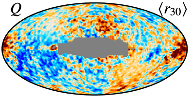
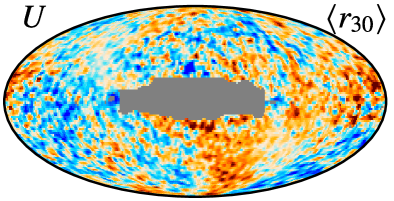
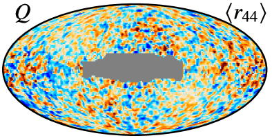
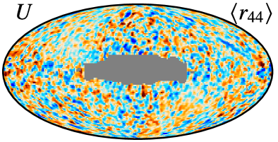
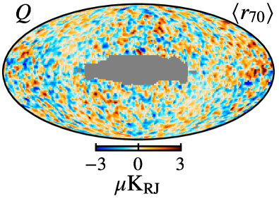
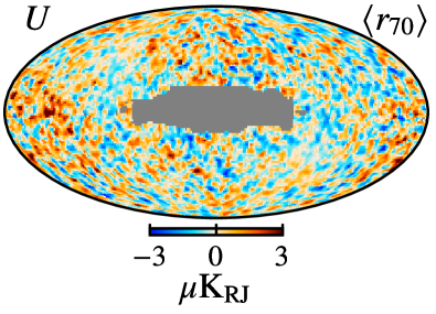
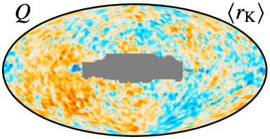
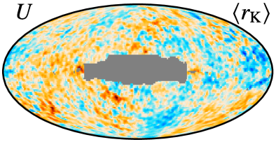
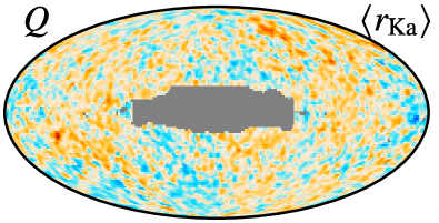
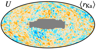
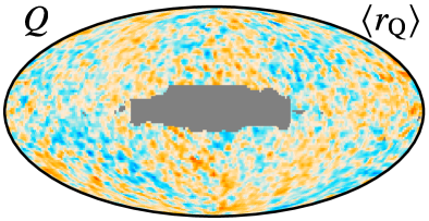
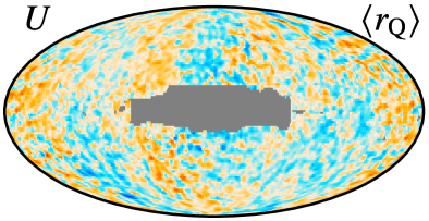
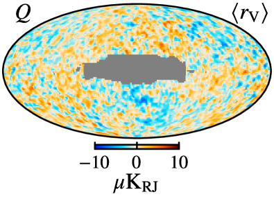
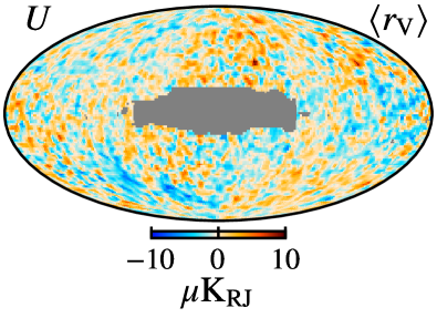
Figure 1: Posterior mean residual maps ($\boldsymbol{r}_{\nu}\thinspace=\thinspace\boldsymbol{d}_{\nu}\thinspace-\thinspace\boldsymbol{s}_{\nu}$) in Stokes $Q$ and $U$ for (from top to bottom) the BeyondPlanck LFI 30, 44, and 70 GHz maps and the WMAP K, Ka, Q, and V bands. All maps are smoothed to a common resolution of $3^{\circ}$ FWHM.

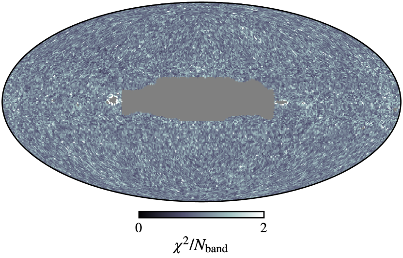
Figure 2: Mean $\chi^{2}/N_{\mathrm{band}}$ of all Gibbs iterations, averaged over Stokes $Q$ and $U$.

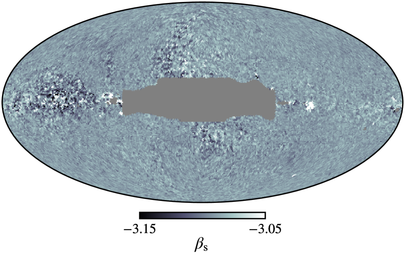
Figure 3: Posterior mean polarized synchrotron spectral index map.

In order to map out the probability distribution of our multidimensional parameter space in a computationally efficient way, we adopt Gibbs sampling (e.g., Gelman et al. 2003). In the Gibbs sampling framework we cycle through each parameter independently, drawing each parameter from a distribution conditional on the values of the other parameters; see, e.g., BeyondPlanck (2022) for details of the much larger BeyondPlanck Gibbs sampler. In the present work, the Gibbs sampler takes the following form,

$$(\@vec{a}_{\mathrm{AME}},\@vec{a}_{\mathrm{s}}) \leftarrow P(a_{\mathrm{AME}},\@vec{a}_{\mathrm{s}}|\@vec{d},\beta_{\mathrm{s}},\beta_{\mathrm{d}})$$ (13)

$$\beta_{\mathrm{s}} \leftarrow P(\beta_{\mathrm{s}}|\@vec{d},\@vec{a}_{\mathrm{AME}},\@vec{a}_{\mathrm{s}},\beta_{\mathrm{d}})$$ (14)

$$\beta_{\mathrm{d}} \leftarrow P(\beta_{\mathrm{d}}).$$ (15)

The two first steps will be detailed below, while the third step just denotes sampling the thermal dust spectral index from its Gaussian prior, as discussed in Sect. 3.2.

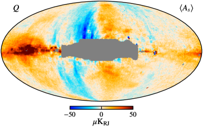
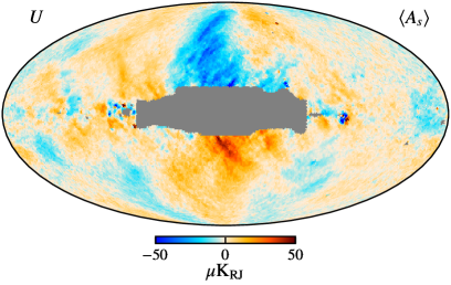
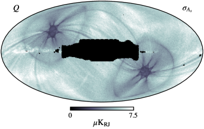
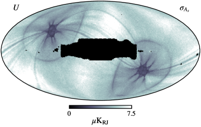
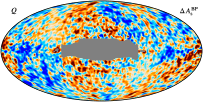
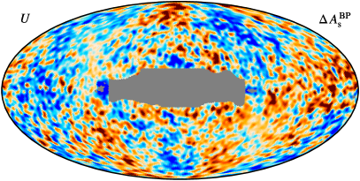
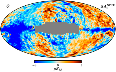
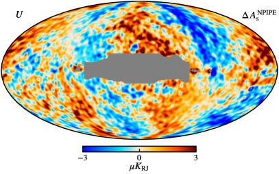
Figure 4: Posterior mean (top) and standard deviation (bottom) maps of the synchrotron amplitude at ${\rm 30\thinspace GHz}$ in Stokes Q (left) and U (right).

Figure 5: Difference between the synchrotron solution derived here and the solution derived in other works. (Top) Difference between the BeyondPlanck synchrotron solution (Svalheim et al. 2022b) and the synchrotron component derived here. (Bottom) Difference between Planck DR4 and the synchrotron component derived here. We note a difference along the Galactic plane, which is likely due to the strong degeneracy between dust and synchrotron emissions in this region. The left and right columns correspond to Stokes $Q$ and $U$, smoothed with a $3^{\circ}$ FWHM Gaussian beam.

4.2 Amplitude sampling

To sample from the conditional distribution for the amplitudes in Eq. (13), we note from Eq. (7) that the signal model is linear in both $\@vec{a}_{\mathrm{AME}}$ and $\@vec{a}_{\mathrm{s}}$. The data model in Eq. (2) may therefore be written in the following compact vector form,

$${d}_{\nu,p}=\@tens{T}_{\nu}\@vec{a}+s_{\mathrm{d},\nu}+{n}_{\nu,p},$$ (16)

where

$$\@vec{a} \equiv\begin{bmatrix}a_{\rm s,0}&\cdots&a_{\rm s,N_{\rm pix}-1}&&a_{\rm AME,1}&\cdots&a_{\rm AME,N_{\rm bands}-1}\end{bmatrix}^{T}$$

$$\@tens{T}_{\nu} \equiv\begin{bmatrix}(\frac{\nu}{\nu_{0,\thinspace{\rm s}}})^{\beta_{{\rm s},0}}&0&0&\delta_{\nu,1}\mathcal{T}_{\mathrm{d},\thinspace 0}&\cdots&\delta_{\nu,n-1}\mathcal{T}_{\mathrm{d},\thinspace 0}\\ 0&\ddots&0&\vdots&\cdots&\vdots\\ 0&0&(\frac{\nu}{\nu_{0,\thinspace{\rm s}}})^{\beta_{{\rm s},N_{\rm pix}-1}}&\delta_{\nu,1}\mathcal{T}_{\mathrm{d},\thinspace N_{\rm pix}-1}&\cdots&\delta_{\nu,n-1}\mathcal{T}_{\mathrm{d},\thinspace N_{\rm pix}-1}\end{bmatrix}.$$

In these expressions, indices for Stokes $Q$ and $U$ parameters are suppressed, but we note that all frequency or component maps should be considered as stacked vectors, $\@vec{a}=\{\@vec{a}^{Q},\@vec{a}^{U}\}$, and matrices are generalized accordingly.

With this notation, $\@vec{d}_{\nu}-\@tens{T}_{\nu}\@vec{a}-\@vec{s}_{\mathrm{d},\nu}=\@vec{n}_{\nu}$, which we assume to be Gaussian distributed with a covariance matrix $\@tens{N}_{\nu}$. Therefore, the likelihood may be written in terms of a standard multivariate Gaussian,

$$\mathcal{L}(\omega)\propto e^{-\frac{1}{2}\sum_{\nu}(\@vec{d}_{\nu}-\@tens{T}_{\nu}\@vec{a}-\@vec{s}_{\mathrm{d},\nu})^{t}\@tens{N}_{\nu}^{-1}(\@vec{d}_{\nu}-\@tens{T}_{\nu}\@vec{a}-\@vec{s}_{\mathrm{d},\nu})}\equiv e^{-\frac{1}{2}\chi^{2}(\@vec{a},\beta)}$$ (17)

When interpreted as a function of $\@vec{a}$ only, this is a strict Gaussian distribution from which a sample may be drawn through the following set of linear equations (see Appendix A of BeyondPlanck 2022 for a pedagogical derivation),

$$\sum_{\nu}\left(\@tens{T}_{\nu,\thinspace j}^{T}\@tens{N}^{-1}_{\nu}\@tens{T}_{\nu,\thinspace j}\right)\boldsymbol{a}=\sum_{\nu}\left(\@tens{T}_{\nu,\thinspace j}^{T}\@tens{N}_{\nu}^{-1}\boldsymbol{(}\@vec{d}_{\nu}-\@vec{s}_{\mathrm{d},\nu})+\@tens{T}_{\nu,\thinspace j}^{T}\@tens{N}_{\nu}^{-1/2}\boldsymbol{\eta}_{j}\right).$$

Here $\boldsymbol{\eta}_{j}$ is a vector of standard Gaussian random variates, $N(0,1)$. This equation may be solved efficiently through standard Conjugate Gradient techniques (Shewchuk 1994).

4.3 Sampling the synchrotron spectral index

Sampling the synchrotron spectral index has been an active topic of analysis throughout the history of both WMAP and Planck . Both the WMAP and Planck Collaborations note difficulties in independently determining $\beta_{\mathrm{s}}$ in polarization and therefore adopted the determination from measurements in total intensity (Bennett et al. 2013; Planck Collaboration IV 2018). Dunkley et al. (2009) assumed a prior of $\beta_{\mathrm{s}}=-3.0\pm 0.3$ from Rybicki & Lightman (1985), finding a mean index of $-3.03\pm 0.04$ in regions of the sky with high signal-to-noise. More recent analyses including S-PASS data find spatial variations in the spectral index ranging between $\beta_{\mathrm{s}}\sim-2.8$ at low Galactic latitudes, and $\beta_{\mathrm{s}}\sim-3.1$ at higher Galactic latitudes, though both are consistent with $\beta_{\mathrm{s}}\sim-3.1$. Additionally, recent work with C-BASS data shows the average synchrotron spectral index between 4.76 and 22.8 GHz to be $\beta_{\mathrm{s}}=-3.1\pm 0.02$ (Harper et al. 2022). Here we explore a variety of priors for with $-3.3<\langle\beta_{\mathrm{s}}\rangle<-3.0$, and assume a nominal prior of $\beta_{\mathrm{s}}=-3.1\pm 0.1$, following the results of Svalheim et al. (2022b).

To sample from Eq. (14), we employ a Metropolis Markov Chain Monte Carlo sampler (Metropolis et al. 1953; BeyondPlanck 2022). Specifically, let $\beta_{j}$ represent the $j$th sample of $\beta_{\rm s}$ in a Markov chain (implicitly suppressing the synchrotron label for readability), and let $T(\beta_{j+1}|\beta_{j})$ be a symmetric stochastic proposal probability distribution, i.e., $T(\beta_{j+1}|\beta_{j})=T(\beta_{j}|\beta_{j+1})$; we adopt a simple Gaussian distribution with a mean of $\beta_{j}$ and a (tunable) standard deviation of $\sigma$.

The Metropolis algorithm is then given by the following steps: First, the chain is initialized at some parameter value $\beta_{0}$, which can chosen as a good estimate to the parameter $\beta$ is as some random value. Secondly, a random sample is drawn from the proposal distribution, as $\beta_{j+1}\leftarrow T(\beta_{j+1}\mid\beta_{j})$, and define $\omega_{j}=\{\@vec{a}_{\mathrm{AME}},\@vec{a}_{\mathrm{s}},\beta_{j},\beta_{\mathrm{d}}\}$, while keeping all other parameters fixed. In order to decide if the sample should be accepted or rejected, the Metropolis acceptance probability $q$ is computed,

$$q=\frac{\mathcal{L}(\omega_{j+1})}{\mathcal{L}(\omega_{j})}\frac{P(\omega_{j+1})}{P(\omega_{j})},$$ (18)

where $\mathcal{L}(\omega)$ is given by Eq. (17) and $P(\omega)$ denotes a Gaussian prior. Once $q$ is calculated, a random number, $\eta$, is drawn from a uniform distribution $U[0,1]$, and the proposed $\omega_{j+1}$ is accepted if $\eta<q$. If the sample is rejected, set $\omega_{j+1}=\omega_{j}$. This procedure is repeated until convergence.

An intuitive observation regarding the Metropolis method is that all samples with a higher posterior probability are accepted, while some samples with a lower posterior probability are accepted. By accepting with a probability given by the ratio of the sample posteriors, the density of samples within a given parameter volume is proportional to the underlying probability density. In this work the proposal probability distribution is Gaussian with a width $\sigma$ determined by the standard deviation of the Gaussian prior distribution. An ensemble of Gaussian priors is used in this analysis to explore the effect of the prior on the final results.

5 Results

We are now ready to present the results derived by applying the Gibbs sampler described in Sect. 4 to the data summarized in Sect. 2. Unless otherwise noted, the default synchrotron spectral index prior is $\beta_{\mathrm{s}}=-3.1\pm 0.1$. For each chain, 500 full Gibbs samples are generated. Between each main sample, we recall that the LFI frequency maps are replaced by different BeyondPlanck samples to marginalize over systematic effects, as discussed in Sect. 2.

5.1 Goodness-of-fit

Before examining the details of each emission component, we consider the overall goodness-of-fit of our data model. Figure 1 shows mean residual maps for each frequency map on the form $\@vec{r}_{\nu}=\@vec{d}_{\nu}-\@tens{T}_{\nu}\@vec{a}-\@vec{s}_{\mathrm{d},\nu}$ for both LFI and WMAP. The gray region indicates the analysis mask discussed in Sect. 2. Generally we observe an excellent fit in terms of Galactic signal suppression; the Galactic plane is only barely visible at the level of a few microkelvin in the LFI 30 GHz and WMAP K-band. However, at higher latitudes there are clear large-scale residuals at the level of $\lesssim 3\thinspace\mu{\rm K}$ for LFI and $\lesssim 5\thinspace\mu{\rm K}$ for WMAP with a clear instrumental origin; for a detailed discussion of these structures, we refer the interested reader to Jarosik et al. (2007), BeyondPlanck (2022), Svalheim et al. (2022b), and Watts et al. (2022).

It is worth noting that the LFI residual maps shown in Fig. 1 appear significantly different from the corresponding maps in the main BeyondPlanck analysis. The reason for this is, as discussed earlier, that the WMAP K-band channel is excluded from the latter analysis. And from this plot we can intuitively understand why: The high signal-to-noise of the WMAP K-band heavily influences the fit of the Planck 30 GHz band, and potential uncontrolled systematic effects in the K-band may therefore compromise the LFI data themselves. We also note that the 30 GHz and K-band residuals are morphologically similar, but with opposite signs, indicating good agreement in terms of the Galactic signal, but with significantly different large-scale scanning-induced systematics. For the main BeyondPlanck analysis, which focuses on LFI, it is therefore clear why the K-band is omitted—while in the current paper, we want to establish a joint estimate between LFI and WMAP, and we want to maximize our signal-to-noise ratio, and we therefore include all data.

Figure 2 shows a corresponding $\chi^{2}$ map, which has been normalized by the number of bands. At this level, we observe very little discernible structure, except for small excesses very near the mask, indicating that the adopted mask indeed performs well.

5.2 Synchrotron component

Next we examine the derived synchrotron posterior component maps. Figure 3 shows the posterior mean map for the synchrotron spectral index, and we recall that the prior in this case is $\beta_{\mathrm{s}}=-3.1\pm 0.1$. Overall we see that $\beta_{\rm s}$ is very close to the prior mean over large portions of the sky, though we can clearly see the impact from the likelihood in some high signal-to-noise regions of the sky. In particular, we note significant deviations from the prior along the Northern Galactic Spur, in the Fan Region, and along the Galactic Plane, in agreement with Svalheim et al. (2022b). However, by far the most important conclusion to be drawn from this figure is the fact that even the combination of LFI and WMAP has very little constraining power compared to the prior with respect to the spectral index of synchrotron emission, and all results that depends on this will necessarily be sensitive to the assumed prior. In the following, we therefore consider the synchrotron index prior mean as a free hyperparameter, and all main results will be plotted as a function of this parameter.

Next, the synchrotron Stokes $Q$ and $U$ amplitude components are summarized in the form of posterior mean (top panels) and standard deviation (bottom panels) maps in Fig. 5. Figure 5 shows difference maps between the synchrotron amplitude map derived in this paper and those generated by the BeyondPlanck (top row) and Planck DR4 (bottom row) pipelines. We find excellent agreement with the different pipelines to around the $3\leavevmode\nobreak\ \thinspace\mu$K_RJ level. The most dominant differences are systematic in nature. In particular, we note that the main difference between the BeyondPlanck and current analysis is the addition of WMAP K-band, while the difference between the current analysis and the Planck DR4 additionally highlights the difference between the end-to-end Bayesian global approach (BeyondPlanck 2022) and the classic frequentist single-channel approach (Planck Collaboration Int. LVII 2020b).

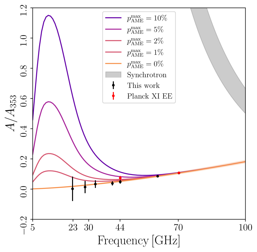
Figure 6: Fitted AME amplitudes for a synchrotron prior of $\beta{\rm s}\sim N(-3.1,0.1)$, with various models for different levels of $p_{\rm AME}^{\mathrm{max}}$ overplotted as colored curves. The red points are taken from Planck Collaboration XI (2020).

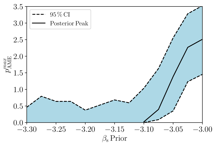
Figure 7: $95\thinspace\%$ confidence intervals for $p_{\rm AME}^{\rm max}$ as a function of the $\beta_{\rm s}$ prior mean.

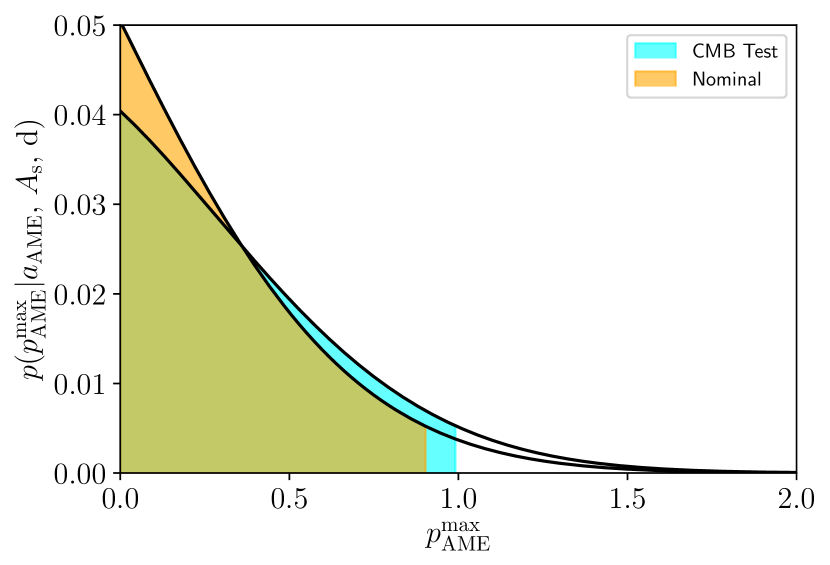
Figure 8: Comparison of likelihood slices for $p_{\rm AME}^{\rm max}$ for a synchrotron prior of $\beta_{\rm s}\thinspace\sim\thinspace N(-3.1,0.1)$ with (blue) and without (orange) additional CMB fluctuations.

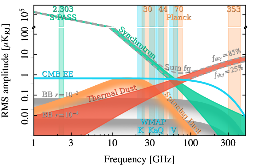
Figure 9: Polarization spectrum in the microwave frequency range. In addition to the traditional spectrum which only includes thermal dust and synchrotron emission, an AME (spinning dust) component is added here with a maximum polarization fraction of $1\thinspace\%$. The thermal dust and synchrotron spectra are determined by results from BeyondPlanck LFI analysis (Svalheim et al. 2022b). The cyan and orange vertical bands correspond to the WMAP  and Planck bands respectively.

5.3 Constraints on AME polarization

Finally, we are ready to present the main results of the current paper, namely constraints on polarized AME emission, and we start the linear amplitude parameters, $\@vec{a}_{\mathrm{AME}}$. As an example, these are shown in Fig. 6 for a synchrotron prior of $\beta_{\mathrm{s}}=-3.1\pm 0.1$. For convenience, we normalize $\@vec{a}_{\mathrm{AME}}$ with respect to the 353 GHz channel, and we plot the sum of the thermal dust emission and AME, with different AME polarization fractions marked as colored curves, ranging between 0 and 10 %.

As discussed in Sect. 3.2, AME amplitudes are not fit at LFI 70 GHz and WMAP V-band as these bands are assumed to be fully described by synchrotron and thermal dust emission. However, Planck Collaboration XI (2020) performed a similar thermal dust emission fit for LFI 70 and 44 GHz, and found good agreement with the SED at 70 GHz. Their 44 GHz result fits shows a slight excess, while in this work we find that the template amplitude fit for BeyondPlanck 44 GHz (and WMAP Q-band) is also consistent with the thermal dust SED alone, at least for a synchrotron prior of $\beta_{\mathrm{s}}=-3.1\pm 0.1$. Also for the lower frequency bands we find results consistent with nonpolarized AME, but with large uncertainties.

To constrain the corresponding AME polarization fraction, we map out the corresponding posterior distribution defined by the change-of-variables in Eq. (10). We create a grid of potential polarized AME SEDs for different polarization fractions, $s_{\nu}(p_{\rm AME})$, and calculate a log-likelihood given by

$$-2\ln\mathcal{L}(p_{\rm AME})=\sum_{\nu}\left(\frac{(\hat{a}_{\nu}-s_{\nu}(p_{\rm AME}))^{2}}{\sigma_{a,\nu}^{2}}\right)^{2}.$$ (19)

Uncertainties in the thermal dust SED are taken into account by averaging over random draws from the MBB parameters as described in Sect. 3. Slices of the full posterior distribution for each of the $\beta_{\rm s}$ priors are shown in Fig. 7, showing the 95 % confidence interval for $p_{\mathrm{AME}}^{\rm max}$, as well as the posterior peak. The nominal case (shown in the form of SED constraints in Fig. 6) is shown in Fig. 8 in orange. In this particular case, we find that the posterior peaks below 0 % with an upper limit of $p_{\mathrm{AME}}^{\rm max}<1.0\thinspace\%$ at the $95\thinspace\%$ confidence level.

However, as shown in Sect. 5.2, the current data set has very little constraining power with respect to $\beta_{\mathrm{s}}$. We therefore repeat the above calculations for a grid of $\beta_{\mathrm{s}}$, allowing the prior mean to range between $\beta=-3.3$ and $\beta=-3.0$. The results from these analyses are summarized in Fig. 7. Here we see that for any $\beta_{\mathrm{s}}\lesssim-3.1$, the distributions are consistent with a vanishing AME polarization fraction, while for flatter indices a nominal positive detection emerges. The most likely explanation for this is that synchrotron emission is oversubtracted by the flat spectral index, and this may be countered by adding a spurious polarized AME component.

Figure 7 summarizes this in the form of the 95 % confidence region as a function of the $\beta_{\mathrm{s}}$ prior mean. Here we find that the typical upper limit is $p_{\mathrm{AME}}^{\rm max}\lesssim 1.0\thinspace\%$ at 95 % confidence for $\beta_{\mathrm{s}}\lesssim-3.1$, while for $\beta_{\mathrm{s}}=-3.0$, there is a nominal detection of polarized AME with $p_{\mathrm{AME}}=2.5\pm 1.0\thinspace\%$ at 95 % confidence.

5.4 Impact of CMB fluctuations

To determine the validity of our assumption to ignore the CMB component in Sect. 3.2, we run our analysis on the same set of data, but with an additional CMB component added to each frequency map. This allows us to estimate the affect the CMB component has on our $p_{\rm AME}^{\rm max}$ constraints.

The CMB component is generated using healpy’s (Zonca et al. 2019) synfast routine, using the Planck best-fit $\Lambda$CDM power spectrum (Planck Collaboration V 2020). The results are shown in Fig. 8, where we show the $p_{\rm AME}^{\rm max}$ posterior slices of the fiducial analysis in orange and the fiducial-plus-CMB analysis in cyan. We see that an additional set of CMB fluctuations increases the upper limits on $p_{\rm AME}^{\rm max}$ by 10–$15\thinspace\%$. As a result, the main limits quoted in paper are likely overestimated, and therefore conservative, as the addition of unmodeled CMB fluctuations lead to slightly weaker constraints.

6 Summary

We have presented the first constraints on large-scale polarized AME derived based on the combination of Planck LFI and WMAP polarization measurements. These constraints are derived within the context of the BeyondPlanck framework, which allows for detailed propagation of systematic errors; the current work is an explicit example of how the BeyondPlanck Monte Carlo frequency map ensembles may be used for error propagation in external analyses. However, we do note that only Planck LFI data are currently processed through this machinery, while traditionally processed maps are employed for WMAP. The effect of this mismatch is seen in various residual and difference maps, clearly demonstrating the presence of instrumental systematic effects in one or both experiments. Work is currently on-going to reprocess the WMAP data jointly with LFI (Watts et al. 2022), but for now we note that the two experiments agree very well in terms of Galactic estimates, even if their instrumental residuals differ. We also note that the $\chi^{2}$ of our fits is excellent, which indicates that systematic errors are small compared to the noise level of each experiment.

We find that the LFI and WMAP data only have limited constraining power with respect to the spectral index of polarized synchrotron emission, and any constraint on the AME polarization fraction is significantly affected by the choice of synchrotron spectral index prior: The current data set is simply not able to robustly and simultaneously constrain polarized AME and synchrotron emission. As a result, we choose to report a limit on the AME polarization fraction that is explicitly $\beta_{\mathrm{s}}$-dependent. Specifically, for $\beta_{\mathrm{s}}\lesssim-3.1$, we find an upper limit of $p_{\mathrm{AME}}^{\rm max}\lesssim 0.6\thinspace\%$ at 95 % confidence, while for $\beta_{\mathrm{s}}\gtrsim-3.1$ there is formally a positive detection of polarized AME power.

The maximum polarization fraction of $3.5\leavevmode\nobreak\ \%$ (for $\beta_{\mathrm{s}}=-3.0$) derived here is in good agreement with and more stringent than the large-scale Macellari et al. (2011) limit of $p_{\mathrm{AME}}<5\%$. Our upper limit also agrees with more stringent upper limits placed in individual molecular cloud complexes, such as those from Battistelli et al. (2006); Génova-Santos et al. (2017); Poidevin et al. (2019), though we emphasize that the AME may be significantly less polarized than the theoretical maximum in these regions based on the magnetic field geometry and level of coherence within the beam and along the line of sight. The nondetection of polarization is in agreement with spinning dust emission theory, driven either by PAHs or nanosilicate grains, but we do not have the sensitivity to discriminate between models with modest levels of polarization and models which predict no polarization. AME driven by emission mechanisms which have polarization fractions of greater than a few percent, such as spinning iron grains (Hoang et al. 2016), are excluded.

We do note that both Planck 2018 (Planck Collaboration V 2020) and BeyondPlanck (BeyondPlanck 2022; Svalheim et al. 2022b) prefer a steep spectral index of $\boldsymbol{\beta_{\mathrm{s}}}\approx-3.3$ at high Galactic latitudes. However, those analyses consider only LFI data, and are therefore susceptible to even stronger degeneracies than what is observed in the current analysis, which also includes WMAP data. It is conceivable that the steep spectral index they observe is partially caused by polarized AME. Another complication is the possibility of curvature in the synchrotron SED, which has not been addressed in the current analysis.

The only way to actually break these degeneracies is through additional high signal-to-noise observations, both by ground-based low-frequency experiments such as C-BASS (Jew et al. 2019), S-PASS (Carretti et al. 2019), QUIJOTE (Génova-Santos et al. 2015), and by next-generation large-scale experiments such as Simons Observatory (Ade et al. 2019) and CMB-S4 (Abazajian et al. 2019). Indeed, we would argue that high-sensitivity characterization of the low-frequency polarized foreground should be a primary objective for near-term CMB experiments, as the complexity of this frequency range can have dramatic consequences for next-generation CMB B-mode satellite experiments.

This is illustrated in Fig. 9, which provides an overview of the polarized microwave sky from 1 to 500 GHz. Green and red bands show synchrotron and thermal dust emission as constrained by BeyondPlanck (Svalheim et al. 2022b), while the orange curve shows the conservative upper limit on polarized AME for a synchrotron spectral index prior of $\boldsymbol{\beta_{\mathrm{s}}}=-3.1\pm 0.1$, namely $p_{\mathrm{AME}}^{\rm max}\lesssim 1.0\thinspace\%$. Clearly, the presence of a polarized AME component with an amplitude this level would be critically important for any future B-mode experiments. In sum, the current analysis serves as a useful reminder about how little is still known about low-frequency polarized foregrounds, even after Planck and WMAP, and more data are desperately needed.