Abstract

Suppose that we have a regression problem with response variable $Y\in\mathbb{R}^{d}$ and predictor $X\in\mathbb{R}^{d}$, for $d\geq 1$. In permuted or unlinked regression we have access to separate unordered data on $X$ and $Y$, as opposed to data on $(X,Y)$-pairs in usual regression. So far in the literature the case $d=1$ has received attention, see e.g., the recent papers by Rigollet and Weed [Information & Inference, 8, 619–717] and Balabdaoui et al. [J. Mach. Learn. Res., 22(172), 1–60]. In this paper, we consider the general multivariate setting with $d\geq 1$. We show that the notion of cyclical monotonicity of the regression function is sufficient for identification and estimation in the permuted/unlinked regression model. We study permutation recovery in the permuted regression setting and develop a computationally efficient and easy-to-use algorithm for denoising based on the Kiefer-Wolfowitz [Ann. Math. Statist., 27, 887–906] nonparametric maximum likelihood estimator and techniques from the theory of optimal transport. We provide explicit upper bounds on the associated mean squared denoising error for Gaussian noise. As in previous work on the case $d=1$, the permuted/unlinked setting involves slow (logarithmic) rates of convergence rooting in the underlying deconvolution problem. Numerical studies corroborate our theoretical analysis and show that the proposed approach performs at least on par with the methods in the aforementioned prior work in the case $d=1$ while achieving substantial reductions in terms of computational complexity.

1 Introduction

In their 1971 paper [1] DeGroot et al. considered the following problem: given photographs of $n$ film stars and another set of photographs of the same film stars taken at a younger age, can we identify corresponding pairs of photographs (i.e., belonging to the same film star) based on, e.g., $d$ biometric measurements extracted from each photograph? A specific variant of this problem (illustrated in Figure 1) is studied in the present paper. Let $\mathcal{X}_{n}=\{X_{i}\}_{i=1}^{n}$ and $\mathcal{Y}_{n}=\{Y_{i}\}_{i=1}^{n}$ be given $\mathbb{R}^{d}$-valued ($d\geq 1$) samples of data (e.g., $\mathcal{X}_{n}$ denoting past photographs and $\mathcal{Y}_{n}$ recent photographs) pertaining to a common set of $n$ entities, and suppose that there is a function $f^{*}:\mathbb{R}^{d}\rightarrow\mathbb{R}^{d}$ transforming data in $\mathcal{X}_{n}$ to their matching counterparts in $\mathcal{Y}_{n}$, modulo additive noise, i.e., for some unknown permutation $\pi^{*}$ of $\{1,\ldots,n\}$, we have that

$$Y_{i}=f^{*}(X_{\pi^{*}(i)})+\epsilon_{i},\quad 1\leq i\leq n,$$ (1)

where the $\{\epsilon_{i}\}_{i=1}^{n}$ represent i.i.d. zero-mean additive noise. Note that if $\pi^{*}$ was known, the problem boils down to a standard regression / (non-parametric) function estimation setup. On the other hand, if $f^{*}$ was known, the problem boils down to a standard matching problem [2, 3]. In this paper, both $f^{*}$ and $\pi^{*}$ are assumed to be unknown, and the following tasks are considered:
(T1): (Exact) Permutation recovery, i.e., inferring the permutation $\pi^{*}$ without error,
(T2): Denoising, i.e., the construction of estimators $\{\widehat{f}(X_{i})\}_{i=1}^{n}$ for $\{f^{*}(X_{i})\}_{i=1}^{n}$. Task (T2) will also be studied in a slightly more general setup in which samples of different size, say, $\mathcal{X}_{n}$ and $\mathcal{Y}_{m}$ are observed such that samples in the latter are i.i.d. copies of $Y\overset{\mathcal{D}}{=}f^{*}(X)+\epsilon$ and samples in $\mathcal{X}_{n}$ are i.i.d. copies of $X\sim\mu$ for some suitable probability measure $\mu$ on $\mathbb{R}^{d}$, with $\overset{\mathcal{D}}{=}$ denoting equality in distribution. Adopting the terminology in [4], this generalized setup will be referred to as unlinked regression, whereas the basic setup (1) will be referred to as permuted regression. In the latter case, $\{X_{i}\}_{i=1}^{n}$ will be considered as fixed, unless stated otherwise. Applications. The problem outlined above arises in a series of applications in various domains. In computer vision, a common task is to identify corresponding pairs of images, with one image arising as a distorted image of the other [5]; in this context, the function $f^{*}$ may represent a specific combination of distortions (e.g., scaling, rotations, blur, etc.). Specific instances of (1) that have received considerable attention lately are unlabeled sensing or linear regression with unknown permutation, e.g., [6, 7, 8, 9, 10, 11, 12, 13, 14, 15, 16] in which case $f^{*}$ is an affine transformation (albeit not necessarily from $\mathbb{R}^{d}$ to $\mathbb{R}^{d}$). Among these works, the papers [11, 16] discuss applications in record linkage [17, 18, 19], specifically post-linkage data analysis [20, 21, 22]. The papers [23, 24] consider the case in which $\mathcal{X}_{n}$ and $\mathcal{Y}_{n}$ are points in the unit sphere in $\mathbb{R}^{d}$ and $f^{*}$ is a unitary map with applications in automated translation between different word embeddings. As elaborated in more detail in $\S$3.1 below, the setup (1) also arises in matrix estimation problems, in which a noisy row-permuted version of a matrix, whose columns exhibit the same ordering pattern (decreasing or increasing), is observed. The papers [25, 26, 27] discuss applications in statistical seriation [28] and microbiome data analysis. Finally, model (1) bears a relation to linkage attacks in the literature on data privacy [29, 30]: here, $\mathcal{Y}_{n}$ may represent (anonymized) sensitive data while an adversary holds auxiliary data $\mathcal{X}_{n}$ along with identifiers (e.g., individuals’ names) and tries to leverage the functional relationship between the two data sets to guess the values of the sensitive attributes contained in $\mathcal{Y}_{n}$ for each or a subset of the identifiers.

$$\begin{array}[]{ccccccccc}X_{1}&X_{2}&\ldots&X_{n}&&Y_{1}&Y_{2}&\ldots&Y_{n}\\ \includegraphics[height=25.29604pt]{plots/clooney_young}&\includegraphics[height=25.29604pt]{plots/cruise_young}&&\includegraphics[height=25.29604pt]{plots/hanks_young}&&\includegraphics[height=25.29604pt]{plots/cruise_old}&\includegraphics[height=25.29604pt]{plots/hanks_old}&\ldots&\includegraphics[height=25.29604pt]{plots/clooney_old}\end{array}$$

Figure 1: Illustration of the film stars correspondence problem described in DeGroot et al. [1]. In terms of model (1), one can potentially think of $\{Y_{1},\ldots,Y_{n}\}$ as the image of $\{X_{1},\ldots,X_{n}\}$ under some “morphing” function $f^{*}$, modulo unstructured noise.

Summary of contributions and related work. In a nutshell, the current paper can be seen as an extension of the setup in the papers [31, 32, 4] which consider (variants of) (1) with $d=1$ and $f^{*}$ monotone with known direction of monotonicity (say, non-decreasing). A fundamental question associated with (1) asks for what class of functions $f^{*}$ it is possible to perform tasks (T1) and (T2) in a statistically consistent manner. In fact, even in the absence of noise and the additional requirement that $f^{*}$ be smooth, (T1) is generally hopeless already for $d=1$ as can be seen from a simple example (cf. $\S$2).

In this paper, we establish that (T1) and (T2) can be accomplished if

$$f^{*}=\nabla\psi_{f^{*}}$$

where $\psi_{f^{*}}:\mathbb{R}^{d}\rightarrow\mathbb{R}$ is a strictly convex function. Such functions $f^{*}$ provide a natural generalization of increasing functions for $d=1$ in view of the property that

$$\langle\nabla\psi_{f^{*}}(y)-\nabla\psi_{f^{*}}(x),y-x\rangle>0\quad\text{for all}\;x,y\in\mathbb{R}^{d}.$$

Note that in particular, functions of the form $f^{*}=(f_{1}^{*},\ldots,f_{d}^{*})$ with $f_{j}^{*}$ increasing on $\mathbb{R}$, $1\leq j\leq d$, as studied in [25, 26, 27] are included, corresponding to component-wise separable additive (strictly) convex functions of the form

$$\psi_{f^{*}}(x_{1},\ldots,x_{d})=\textstyle\sum_{j=1}^{d}\psi_{f_{j}^{*}}(x_{j}).$$

Permutation recovery in the presence of noise based on the solution of a linear assignment problem associated with $\mathcal{X}_{n}$ and $\mathcal{Y}_{n}$ is shown to succeed if a certain minimum signal condition similar to conditions in related papers [25, 26, 27, 15] is met. As a byproduct, the result on permutation recovery herein yields the novel insight that the unlabeled sensing problem in [15] can be solved efficiently whenever the unknown linear transformation is positive (semi)-definite.

Regarding the task (T2) of denoising, we leverage a connection to the Brenier theorem in optimal transportation, e.g., [33, 34, 35, 36]. According to this connection, the sample $\mathcal{Y}_{n}$ is thought of as the image of $\mathcal{X}_{n}$ under an optimal transport map $f^{*}=\nabla\psi_{f^{*}}$, contaminated by additive noise. Denoising is achieved via deconvolution of the measure $\frac{1}{n}\sum_{i=1}^{n}\delta_{Y_{i}}$ and subsequent computation of an optimal coupling $\widehat{\gamma}$ between the deconvolution estimate and the measure $\frac{1}{n}\sum_{i=1}^{n}\delta_{X_{i}}$; finally, we take $\{\widehat{f}(X_{i})\}_{i=1}^{n}$ as the so-called barycentric projection of $\widehat{\gamma}$. Deconvolution is based on the Kiefer-Wolfowitz NPMLE for location mixtures [37, 38] and requires knowledge of the noise distribution. The approach developed herein is free of tuning parameters, and directly generalizes to the unlinked regression setting with samples $\mathcal{X}_{n}$ and $\mathcal{Y}_{m}$ of different size described above at the end of the first paragraph. We provide upper bounds on the mean-square denoising error $\frac{1}{n}\sum_{i=1}^{n}\lVert f^{*}(X_{i})-\widehat{f}(X_{i})\rVert_{2}^{2}$ in terms of the Hellinger distance of the Kiefer-Wolfowitz NPMLE to the underlying location mixture generating $\mathcal{Y}_{n}$ and the rate of decay of the noise distribution, the latter being a common ingredient in deconvolution problems. For Gaussian errors, all quantities can be made explicit, yielding rather slow rates of convergence in alignment with prior work [31, 32, 4] on the case $d=1$.

The main innovations of the present work over [31, 32, 4] is the generalization to arbitrary dimension $d$, whereas [31, 32, 4] only consider $d=1$. All three works are based on deconvolution, and a connection to optimal transportation, albeit for $d=1$, is already made in [32]. However, even for $d=1$, we argue that the approach developed in this paper is computationally more appealing than those in [31, 32, 4]. The method in [31] is based on the truncated characteristic function estimator originating in the deconvolution literature and hence entails a tuning parameter. The method in [32] is tuning-free and based on convex optimization; however, their deconvolution procedure involves Wasserstein distance minimization and in turn a non-smooth optimization problem that is less straightforward to solve than the Kiefer-Wolfowitz NPMLE. The method in [4] is based on a non-convex optimization problem.

The theoretical results presented in [31, 32, 4] are of different flavors, and hence not directly comparable. The paper [31] does not provide explicit rates of convergence. The paper [4] is different from [32] in the sense that the former emphasizes on the unlinked regression setting and provides rates for function estimation in the $L_{1}$-distance, whereas [32] studies the mean-squared denoising error in the permuted regression setting (1). For $d=1$, the denoising performance metric in [32] (mean squared error at the $\{X_{i}\}_{i=1}^{n}$) coincides with what is considered in the present paper. The rate herein is slightly slower than the minimax rate shown in [32], but given that both rates decrease only logarithmically in $n$, the gap is not that pronounced. More detailed comparisons are postponed to later sections in this paper. Finally, we would like to mention the paper [39] that studies the setting in [32] under discrete errors.

The approach taken in this paper and the techniques used for its analysis bear various connections to recent developments in the literature on optimal transport, e.g., on the estimation of (smooth) optimal transport maps [40, 41, 42, 43, 44]. Key steps in our proofs are based on adaptations of parts of the analysis in [44, 42, 43]. At a technical level, the main distinction of the present work compared to these earlier works is the convolution setting considered herein.

Paper outline. This paper is organized as follows. Section $\S$2 provides a more detailed discussion of the problem sketched in the introduction, and presents an overview of the technical approach taken. The theoretical properties of that approach are studied in $\S$3 and corroborated with numerical results in $\S$4. A conclusion is provided in $\S$5. Proofs of our results and additional technical details can be found in the Appendix. Notation. For the convenience of the reader, notation that is used frequently in this paper is summarized in the following table.

$\{\theta_{i}^{*}\}_{i=1}^{n}$	unknown location parameters	$f^{*}$	function of interest
$\nu_{n}^{*}$	measure $\frac{1}{n}\sum_{i=1}^{n}\delta_{\theta_{i}^{*}}$	$\psi_{f^{*}}$	convex function associated with $f^{*}$
$\nu_{n}$	measure $\frac{1}{n}\sum_{i=1}^{n}\delta_{Y_{i}}$	$\psi_{f^{*}}^{\star}$	Conjugate of $\psi_{f^{*}}$
$\mu_{n}$	measure $\frac{1}{n}\sum_{i=1}^{n}\delta_{X_{i}}$	$\pi^{*}$	ground truth permutation of $\{1,\ldots,n\}$
$\varphi$	PDF of $\epsilon/\sigma$, $\operatorname{Cov}(\epsilon)=\sigma^{2}I_{d}$	$\Pi^{*}$	permutation matrix corresponding to $\pi^{*}$
$\varphi_{\sigma}$	PDF of $\epsilon$	$\mathcal{P}(n)$	set of permutation matrices of order $n$
$\star$	convolution	$\pi,\Pi$	generic elements of $\mathcal{P}(n)$
$\textsf{f}_{n}=\varphi_{\sigma}\star\nu_{n}^{*}$	average location mixture PDF	$\mathbf{F}$	Fourier transformation (operator)
$\widehat{\textsf{f}}_{n}$	NPMLE of $\textsf{f}_{n}$	$\widehat{g}$	short for $\mathbf{F}[g]$

We often refer to a permutation via the underlying map $\pi$ and the corresponding matrix $\Pi$ in an interchangeable fashion, and accordingly $\mathcal{P}(n)$ may refer to both maps and matrices.

2 Estimation strategy

In this section we describe our estimation procedure for both tasks – (T1) and (T2). We start with a simple example that illustrates the non-identifiability of $f^{*}$ and $\pi^{*}$ in (1) without further assumptions on the structure of $f^{*}$; see Remark 1 below. It turns out that if $f^{*}$ is cyclically monotone (see Section 2.1 where we formally define this notion along with other related concepts) then model (1) is identifiable and consistent estimation can be successfully carried out. To solve the denoising problem (T2) we leverage ideas from the theory of optimal transport and the Kiefer-Wolfowitz NPMLE for location mixtures which is discussed in detail in Section 2.2. We also give our main algorithm (see Algorithm 1) and discuss the computational approach in Section 2.2.

Remark 1.

(A negative example) To gain some insights into the feasibility of tasks (T1) and (T2) given the observation model (1), let us first consider a simple example which shows that recovery of $f^{*}$ or $\pi^{*}$ is generally hopeless even in seemingly benign settings ($d=1$, no noise, $f^{*}$ smooth). Specifically, suppose that $X_{i}=Y_{i}=i/M$, $1\leq i\leq n=M-1$ for $M\geq 2$. Then both pairs $f_{1}^{*}(x)=x$ with $\pi_{1}^{*}(i)=i$, $1\leq i\leq n$, and $f_{2}^{*}(x)=1-x$ with $\pi_{2}^{*}(i)=n-i$, $1\leq i\leq n$, satisfy (1). Clearly, additionally requiring that $f^{*}$ be increasing rules out this ambiguity. In fact, estimation of monotone $f^{*}$ with known direction of monotonicity under the permuted regression setup (1) has been shown to be feasible even in the presence of noise [31, 32, 4]. At the same time, estimation of the direction of monotonicity itself is generally not possible even if $f^{*}$ is linear [45, 46].

2.1 Monotone operators and linear assignment problems

The example above for $d=1$ (and in the absence of noise) provides some useful clues regarding the generalization to arbitrary dimension $d\geq 1$. If $f^{*}$ is known to be increasing, the underlying permutation $\pi^{*}$ is immediately determined by the requirement that $Y_{i}$ must match the corresponding order statistic in $\mathcal{X}_{n}$, i.e., $X_{\pi^{*}(i)}=X_{\text{rank}(i)}$, where $\text{rank}(i)$ denotes the rank of $Y_{i}$ among $\mathcal{Y}_{n}$, $1\leq i\leq n$. It can also be shown that $\pi^{*}$ minimizes the optimization problem

$$\min_{\pi}\frac{1}{2}\sum_{i=1}^{n}|Y_{i}-X_{\pi(i)}|_{2}^{2}=-\max_{\pi}\sum_{i=1}^{n}X_{\pi(i)}Y_{i}+c,\qquad\quad c\mathrel{\mathop{:}}=\frac{1}{2}\sum_{i=1}^{n}(X_{i}^{2}+Y_{i}^{2})$$ (2)

over all permutations $\pi$ of $\{1,\ldots,n\}$. The above problem is a specifically simple instance of the class of linear assignment problems (LAPs) that are of the form

$$\min_{\Pi\in\mathcal{P}(n)}\sum_{i=1}^{n}\sum_{j=1}^{n}\Pi_{ij}C_{ij}=\min_{\Pi\in\mathcal{P}(n)}\mathrm{tr}(C^{\top}\Pi),$$ (3)

where $\mathcal{P}(n)=\{\Pi\in\{0,1\}^{n\times n}:\,\sum_{i=1}^{n}\Pi_{ij}=1,\,1\leq j\leq n,\;\sum_{j=1}^{n}\Pi_{ij}=1,\,1\leq i\leq n\}$ denotes the set of permutation matrices of dimension $n$ and $C=(c_{ij})$ is a cost matrix with entry $(i,j)$ representing the cost associated with the pairing $(i,j)$, $1\leq i,j\leq n$. LAPs (3) constitute a well-studied class of optimization problems that are known as bipartite matching problems in the literature on combinatorial optimization [2]. In light of the celebrated Birkhoff-von Neumann theorem [47], (3) can be solved efficiently via linear programming. Tailored algorithms such as the Hungarian Algorithm [48] and the Auction Algorithm [49] have runtime complexity $O(n^{3})$, and approximate solutions can be obtained via Sinkhorn iterations in time $O(n^{2}\log n)$ [50]; especially simple instances such as (2) in which $C$ has rank one reduce to sorting.

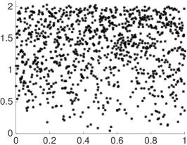
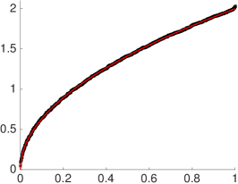
Figure 2: Left: Shuffled Data $\{(X_{i},Y_{i})\}_{i=1}^{n}$. Middle: Sorted Data $(X_{(i)},Y_{(i)})_{i=1}^{n}$ in case of negligible noise; underlying function $x\mapsto f^{*}(x)\mathrel{\mathop{:}}=2\sqrt{x}$ in red. Right: Sorted Data $(X_{(i)},Y_{(i)})_{i=1}^{n}$ in case of substantial noise. The results indicates a serious amount of bias, particularly near the boundaries.

The crucial insight here is that knowing $f^{*}$ is monotone increasing immediately allows us to recover $\pi^{*}$ in the absence of noise via the optimization problem (2). This observation prompts the following generalization. Let $\mathbb{X}^{n}\subset\mathbb{R}^{d}\times\ldots\times\mathbb{R}^{d}$ be a domain containing all possible samples $\mathcal{X}_{n}$. We require that for all $\mathcal{X}_{n}\subset\mathbb{X}^{n}$ and all $n\geq 1$, $f^{*}$ has the property that

$$\min_{\pi}\frac{1}{2}\sum_{i=1}^{n}\lVert Y_{i}-X_{\pi(i)}\rVert_{2}^{2},$$ (4)

is (uniquely) minimized by $\pi=\pi^{*}$, where $Y_{i}=f^{*}(X_{\pi^{*}(i)}),\;1\leq i\leq n$. This requirement can be expressed more succinctly via the notion of (strict) cyclical monotonicity, a notion that arises in the study of monotone operators in convex analysis [51] as well as in optimal transportation [e.g., 52, Definition 2.1], a connection that plays a fundamental role in the developments further below.

Proposition 1.

Without loss of generality, suppose that $\pi^{*}$ equals the identity id permutation. The optimization problem (4) is uniquely minimized by $\pi=\textsf{\emph{id}}$ iff $\Gamma_{f^{*}}:=\{(x,f^{*}(x)):\,x\in\mathbb{X}\}\subset\mathbb{R}^{d}\times\mathbb{R}^{d}$ is a (strictly) cyclically monotone set (with respect to the Euclidean norm), i.e., if for all $k\geq 1$ and all $\{(x_{i},y_{i})\}_{i=1}^{k}\subset\Gamma_{f^{*}}$, it holds that

$$-\sum_{i=1}^{k}\langle x_{i},y_{i}\rangle<\sum_{i=1}^{k}-\langle x_{i+1},y_{i}\rangle,\qquad x_{k+1}\mathrel{\mathop{:}}=x_{1}.$$ (5)

Proposition 1 is obtained by omitting the square terms in the objective as in (2) and decomposing permutations into their disjoint cycles; a formal proof is omitted for the sake of brevity. The following result, due to Rockafellar, precisely characterizes the class of functions $f:\mathbb{R}^{d}\rightarrow\mathbb{R}^{d}$ whose graphs are cyclically monotone.

Theorem 1.

[53] The graph of the sub-differential $\partial\psi$ of a convex function $\psi:\mathbb{R}^{d}\rightarrow\mathbb{R}^{d}$, i.e., $\Gamma_{\partial\psi}:=\{(x,y)\in\mathbb{R}^{d}\times\mathbb{R}^{d}:\psi(z)\geq\psi(x)+\langle z-x,y\rangle\;\forall z\in\mathbb{R}^{d}\}$ is a cyclically monotone subset of $\mathbb{R}^{d}\times\mathbb{R}^{d}$. Moreover, any cyclically monotone subset of $\mathbb{R}^{d}\times\mathbb{R}^{d}$ is contained in such a set.

The subdifferential of a convex function $\psi$ is a monotone operator in the sense that the relation $\{(x,\partial\psi(x)):\,x\in\mathbb{R}^{d}\}$ has the property that $\langle x-z,g_{x}-g_{z}\rangle\geq 0$ for all $x,z\in\mathbb{R}^{d}$ and all $g_{x}\in\partial\psi(x),\,g_{z}\in\partial\psi(z)$, which is in analogy to the fact monotone functions on the real line arise as derivatives of convex functions.

In combination, Proposition 1 and Rockafellar’s theorem above prompt the requirement

$$f^{*}=\nabla\psi_{f^{*}}$$

for a convex function $\psi_{f^{*}}:\mathbb{R}^{d}\rightarrow\mathbb{R}^{d}$. Working with gradients instead of subdifferentials is needed in order to ensure that $f^{*}$ is actually a map from $\mathbb{R}^{d}$ to $\mathbb{R}^{d}$ even though the distinction is somewhat minor in light of the fact that convex functions are differentiable (Lebesgue) almost everywhere.

For the purpose of permutation recovery (T1) and in turn for strict cyclical monotonicity to hold, we need to impose the additional requirement that $\psi_{f^{*}}$ be strictly convex, i.e., the strengthened first-order convexity condition

$$\psi_{f^{*}}(z)>\psi_{f^{*}}(x)+\langle\nabla\psi_{f^{*}}(x),z-x\rangle\quad\forall\;x,z\in\mathbb{R}^{d},\;x\neq z.$$ (6)

Note that $\nabla\psi_{f^{*}}:\mathbb{R}^{d}\rightarrow\mathbb{R}^{d}$ is injective if and only if (6) holds. In the presence of noise, strict convexity will further be strengthened to strong convexity (cf. Proposition 2 in $\S$3 below).

2.2 A path towards denoising (T2) via optimal transportation

Gradients of convex functions are also known as Brenier maps in the field of optimal (measure) transportation [e.g., 34, 35, 36]. Specifically, for random variables $U\sim\rho$ and $V\sim\tau$ with $\rho$ and $\tau$ absolutely continuous with respect to the Lebesgue measure on $\mathbb{R}^{d}$ such that $\operatorname{\mathbf{E}}_{U\sim\rho}[\lVert U\rVert_{2}^{2}],\operatorname{\mathbf{E}}_{V\sim\tau}[\lVert V\rVert_{2}^{2}]$ are both finite, Brenier’s theorem (in short) states that the minimization problem

$$\inf_{T}\,\frac{1}{2}\operatorname{\mathbf{E}}_{U\sim\rho}[\lVert U-T(U)\rVert_{2}^{2}],$$

over all measurable functions $T$ such that $T(U)\sim\tau$ has a solution $T^{\ast}=\nabla\psi_{T^{*}}$ for a convex function $\psi_{T^{*}}$ with $T^{*}$ being uniquely determined almost everywhere. Moreover, the solution of the reverse problem in which $\tau$ is optimally transported to $\rho$ in the above sense is the optimal transport map given by $\nabla\psi_{T^{*}}^{\star}$ with $\psi_{T^{*}}^{\star}$ denoting the Legendre-Fenchel conjugate of $\psi_{T^{*}}$; we refer to Appendix G for a more detailed background and references.

Linear assignment problems of the form (2) and $\eqref{eq:permutation_min_general}$ can be interpreted as specific discrete optimal transport problems between the atomic measures

$$\mu_{n}:=\textstyle\frac{1}{n}\textstyle\sum_{i=1}^{n}\delta_{X_{i}},\qquad\text{and}\qquad\nu_{n}:=\frac{1}{n}\sum_{i=1}^{n}\delta_{Y_{i}}.$$

The requirement that $\mu_{n}(T^{-1}(Y_{i}))=1/n$, $1\leq i\leq n$, immediately implies that the resulting optimal transport problem seeks for an optimal pairing $\{(X_{\pi(i)},Y_{i})\}_{i=1}^{n}$ over all permutations $\pi$ of $\{1,\ldots,n\}$.

The connection to optimal transportation turns out to be fruitful since it suggests a natural approach for the task of denoising (T2), i.e., the construction of estimators $\{\widehat{f}(X_{i})\}_{i=1}^{n}$ of $\{f^{*}(X_{i})\}_{i=1}^{n}$ under the permuted regression model (1). Note that solving the linear assignment problem (4) to find an optimal collection of $(X,Y)$-pairs is not suitable for this task in general since all noise inherent in the $\{Y_{i}\}_{i=1}^{n}$ is retained (cf. Figure 2). In fact, we are interested in the pairings $\{(X_{i},\theta_{i}^{*})\}_{i=1}^{n}$ with $\theta_{i}^{*}=f(X_{i}^{*})$, $1\leq i\leq n$, which corresponds to the optimal transportation problem between $\mu_{n}$ and $\nu_{n}^{*}:=\frac{1}{n}\sum_{i=1}^{n}\delta_{\theta_{i}^{*}}$. Since the latter is not given — in fact, it corresponds to the target to be recovered — suggests the need for its estimation. Below, we shall present an atomic estimator $\widehat{\nu}$ of $\nu_{n}^{*}$ of the form

$$\widehat{\nu}:=\textstyle\sum_{j=1}^{p}\widehat{\alpha}_{j}\delta_{\widehat{\theta}_{j}}$$

with atoms $\{\widehat{\theta}_{j}\}_{j=1}^{p}\subset\mathbb{R}^{d}$ and masses (i.e., positive numbers summing to one) $\{\widehat{\alpha}_{j}\}_{j=1}^{p}$. Since $p\neq n$ in general, there does not exist a transport map between $\mu_{n}$ and $\widehat{\nu}$. However, the Kantorovich problem, a relaxation of the optimal transportation problem (cf. Appendix G), can be used to obtain a proxy as follows. The Kantorovich problem is given by the optimization problem

$$\min_{\gamma\in\Pi(\mu_{n},\widehat{\nu})}\int\int\frac{1}{2}\lVert x-\theta\rVert_{2}^{2}\;d\gamma(x,\theta),$$ (7)

where the minimum is over all couplings $\gamma$ of $\mu_{n}$ and $\widehat{\nu}$, i.e., all probability measures on the set $\{X_{i}\}_{i=1}^{n}\times\{\widehat{\theta}_{j}\}_{j=1}^{p}$ whose marginal distributions are given by $\mu_{n}$ and $\widehat{\nu}$, respectively.

Let $\widehat{\gamma}$ denote a minimizer of (7). We then use the estimator

$$\widehat{f}(X_{i})\mathrel{\mathop{:}}=\operatorname{\mathbf{E}}_{(\theta,X)\sim\widehat{\gamma}}[\theta|X=X_{i}]=\frac{\int_{\theta}\theta\;d\widehat{\gamma}(\theta,X_{i})}{{\int_{\theta}\;d\widehat{\gamma}(\theta,X_{i})}}=\frac{\int_{\theta}\theta\;d\widehat{\gamma}(\theta,X_{i})}{\mu_{n}(\{X_{i}\})},\quad 1\leq i\leq n,$$ (8)

i.e., the conditional expectation of $\theta$ given $X=X_{i}$, $1\leq i\leq n$, resulting from the optimal coupling $\widehat{\gamma}$. The map $x\mapsto\operatorname{\mathbf{E}}_{(X,\theta)\sim\widehat{\gamma}}[\theta|X=x]$, $x\in\mathcal{X}_{n}$, is usually referred to as the barycentric projection of $\widehat{\gamma}$ in the optimal transport literature [54, Definition 2].

In order to finalize the outline of our approach for task (T2), which is summarized in Algorithm 1, it remains to present a specific estimator $\widehat{\nu}$ of $\nu_{n}^{*}$. Let $\varphi$ denote the density of the i.i.d. standardized noise terms $\{\epsilon_{i}/\sigma\}_{i=1}^{n}$, where we assume that $\operatorname{\mathbf{E}}[\epsilon_{1}]=0$ and $\operatorname{Cov}(\epsilon_{1})=\sigma^{2}I_{d}$, for $\sigma>0$. Then the average density of the $\{Y_{i}\}_{i=1}^{n}$ is given by the location mixture density $\textsf{f}_{n}:=\varphi_{\sigma}\star\nu_{n}^{*}$ with $\star$ denoting convolution and $\varphi_{\sigma}(\cdot):=\sigma^{-d}\varphi(\cdot/\sigma)$, i.e.,

$$\textsf{f}_{n}(y)=\int\varphi_{\sigma}(y-\theta)\;d\nu_{n}^{*}(\theta)=\frac{1}{n}\sum_{i=1}^{n}\varphi_{\sigma}(y-\theta_{i}^{*}),\quad y\in\mathbb{R}^{d}.$$

We propose to estimate $\textsf{f}_{n}$ via the Kiefer-Wolfowitz nonparametric maximum likelihood estimator (NPMLE) [37, 38] given by

$$\inf_{\textsf{f}\in\mathcal{F}_{\varphi,\sigma}}-\sum_{i=1}^{n}\log\textsf{f}(Y_{i}),\quad\mathcal{F}_{\varphi,\sigma}\mathrel{\mathop{:}}=\left\{\textsf{f}=\int\varphi_{\sigma}(y-\theta)d\nu(\theta):\;\,\nu\,\,\text{distribution on $\mathbb{R}^{d}$}\right\}.$$ (9)

$\begin{array}[]{l}\text{{Inputs}: $\mathcal{X}_{n}$, $\mathcal{Y}_{m}$, $\varphi_{\sigma},\mathbb{G}$.}\\[4.30554pt] \text{1. Solve problem \eqref{eq:Kiefer_Wolfowitz_approx1}:}\\[2.15277pt] \text{$\leadsto$ $\widehat{\nu}=\sum_{j=1}^{p}\widehat{\alpha}_{j}\delta_{\widehat{\theta}_{j}}$}\\[4.30554pt] \text{2. Compute an optimal coupling}\\ \text{$\quad$ between $\mu_{n}$ and $\widehat{\nu}$ via the}\\ \text{$\quad$ linear program \eqref{eq:Kantorovich_finite}.}\\[2.15277pt] \text{$\leadsto$ $\widehat{\Gamma}\in\mathbb{R}_{+}^{n\times p}$.}\\[4.30554pt] \text{{Return} $\widehat{f}(X_{i})=n\sum_{j}\widehat{\Gamma}_{ij}\widehat{\theta}_{j}$},\\ \text{$\qquad\quad\;\,$ $1\leq i\leq n$.}\\[129.16626pt] \end{array}$

Algorithm 1 Denoising for Permuted or Unlinked Regression

Left figure: $\nu_{n}^{*}=\frac{1}{n}\sum_{i=1}^{n}\delta_{\theta_{i}^{*}}$ with $\theta_{i}^{*}=2\sqrt{X}_{i}-0.5$, $1\leq i\leq n$, with $\mathcal{X}_{n}=\{0.1,0.2,\ldots,0.8\}$. The solid black line drawn over the vertical axis represents the mixture density $\textsf{f}_{n}=\nu_{n}^{*}\star\varphi_{\sigma}$. Right figure: Estimated mixture density $\widehat{\textsf{f}}_{n}$ and mixing measure $\widehat{\nu}$ (blue). The resulting optimal coupling $\widehat{\Gamma}$ between $\mu_{n}$ and $\widehat{\nu}$ is represented by purple dots (with sizes proportional to the corresponding entry of $\widehat{\Gamma}$. Solid black line: Function estimate $\widehat{f}$ obtained by constant interpolation based on $\{(X_{i},\widehat{f}(X_{i}))\}_{i=1}^{n}$.

Even though the optimization problem (9) is infinite-dimensional, it can be shown that a solution $\widehat{\textsf{f}}_{n}$ exists, and that the associated mixing measure $\widehat{\nu}$ is atomic with a finite number of atoms [38, 56]. We shall use $\widehat{\nu}$ as an estimator of $\nu_{n}^{*}$ that is then plugged into the Kantorovich problem (7). Note that the Kiefer-Wolfowitz problem assumes knowledge of the density $\varphi_{\sigma}$, i.e., the noise distribution. This assumption is common in deconvolution problems [57] as encountered here; in fact, without any knowledge about the noise distribution, deconvolution problems are generally ill-defined. The assumption of known $\sigma$ can potentially be relaxed (cf. $\S$5). Unlinked Regression. The estimator (8) remains applicable in the unlinked regression setting in which $\mathcal{X}_{n}$ and $\mathcal{Y}_{m}$ are of different sizes $n\neq m$ as described in the introduction with the elements of $\mathcal{Y}_{m}$ being i.i.d. as $Y\overset{\mathcal{D}}{=}f^{*}(X)+\epsilon$ with $X\sim\mu$ for some absolutely probability measure $\mu$ supported on a compact subset of $\mathbb{R}^{d}$ and $f^{*}=\nabla\psi_{f^{*}}$ for $\psi_{f^{*}}$ convex. In fact, $\mathcal{Y}_{m}$ can be used to obtain an estimator $\widehat{\nu}$ of $\frac{1}{n}\sum_{i=1}^{n}\delta_{f^{*}(X_{i})}$ as before via (9), and all subsequent steps in Algorithm 1 can be executed. The rates of convergence for the denoising error are almost identical to the permuted regression setting with $n=m$ as long as $n\asymp m$, cf. $\S$3.2. Computation. Algorithm 1 requires computation of the Kiefer-Wolfowitz NPMLE, the Kantorovich problem (7), and finally the barycentric projections (8). The Kiefer-Wolfowitz problem can be reformulated as a (non-convex) finite mixture likelihood optimization problem, and then solved via the EM algorithm [58]. Instead, in order to preserve convexity, we approximate the solution of (9) via the finite-dimensional optimization problem

$$\inf_{\textsf{f}\in\mathcal{F}_{\varphi,\sigma}^{\mathbb{G}}}-\sum_{i=1}^{n}\log\textsf{f}(Y_{i}),\quad\mathcal{F}_{\varphi,\sigma}^{\mathbb{G}}\mathrel{\mathop{:}}=\left\{\textsf{f}=\int\varphi_{\sigma}(y-\theta)d\nu(\theta):\;\,\nu\,\,\text{distribution on $\mathbb{G}$}\right\},$$ (10)

where $\mathbb{G}$ is a finite set of points in $\mathbb{R}^{d}$. Problem (10) can be rewritten as

$$\inf_{\alpha\in\Delta^{|\mathbb{G}|}}-\sum_{i=1}^{n}\log\left(\sum_{j=1}^{|\mathbb{G}|}\alpha_{j}\varphi_{\sigma}(Y_{i}-\theta_{j})\right),$$ (11)

where $\Delta^{r}\mathrel{\mathop{:}}=\{x\in\mathbb{R}_{+}^{r}:\sum_{j=1}^{r}x_{j}=1\}$ denotes the probability simplex in $\mathbb{R}^{r}$, $r\geq 1$. There is a variety of convex optimization algorithms that can be used to solve (11). Our experiments are based on a primal-dual interior point method [59] that yields fast and highly accurate results even if $|\mathbb{G}|$ includes several thousand points. Regarding $\mathbb{G}$, our default is choice is $\mathbb{G}=\mathcal{Y}_{n}$ for $d\geq 2$ and $\mathbb{G}$ being a set of $g_{n}$ linearly spaced points in the interval $[\min_{i}Y_{i},\max_{i}Y_{i}]$ with $g_{n}=n$ or $g_{n}=n^{1/2}$. In the paper [60] it is shown that the latter choice suffices to ensure comparable statistical performance to the solution of the infinite-dimensional problem (9).

Solving (10) yields the estimator $\widehat{\nu}=\sum_{j=1}^{p}\widehat{\alpha}_{j}\delta_{\widehat{\theta}_{j}}$, where $\{\widehat{\alpha}_{j}\}_{j=1}^{p}$ represent the non-zero entries of the resulting minimizer of (11) and $\{\widehat{\theta}_{j}\}_{j=1}^{p}\subseteq\mathbb{G}$ represent the corresponding atoms. Computing an optimal coupling between the two finitely supported measures $\mu_{n}$ and $\widehat{\nu}$ according to problem (7) amounts to solving the linear program

$$\min_{\Gamma\in\mathbb{R}_{+}^{n\times p}}\mathrm{tr}(C^{\top}\Gamma)\quad\text{subject to}\;\sum_{i=1}^{n}\Gamma_{ij}=\widehat{\alpha}_{j},\;1\leq j\leq p,\;\;\,\sum_{j=1}^{p}\Gamma_{ij}=\frac{1}{n},\;1\leq i\leq n,$$ (12)

where $C=(\lVert X_{i}-\widehat{\theta}_{j}\rVert_{2}^{2}/2)_{1\leq i\leq n,1\leq j\leq p}$, and the row and column sum constraints represent the requirements on the two marginal distributions. Solving (12) exhibits similar computational complexity to the linear assignment problem (3). For the numerical examples presented in this paper, we used the routine cplexlp in CPLEX [61]. Fast approximate solution can be obtained via Sinkhorn iterations [50]. For $d=1$, problem (12) becomes considerably simpler due to the natural ordering of the real line, and can be solved in time $O(n+p)$ via the so-called “Northwest Corner Rule” [33, $\S$3.4.2] after sorting the $\{X_{i}\}_{i=1}^{n}$ and $\{\widehat{\theta}_{j}\}_{j=1}^{p}$.

Finally, given a minimizer $\widehat{\Gamma}$ of (12), the barycentric projections (8) can be computed as

$$\widehat{f}(X_{i})=\sum_{j=1}^{p}\widehat{\Gamma}_{ij}\widehat{\theta}_{j}\,\Big{/}\sum_{j=1}^{p}\widehat{\Gamma}_{ij}=n\sum_{j=1}^{p}\widehat{\Gamma}_{ij}\widehat{\theta}_{j},\quad 1\leq i\leq n.$$

3 Main results

In this section, we first analyze permutation recovery (T1) based on the linear assignment problem in (4) with the distinction that $\{Y_{i}\}_{i=1}^{n}$ may be contaminated by Gaussian additive noise, i.e., $Y_{i}=f(X_{\pi^{*}(i)})+\epsilon_{i}$, $1\leq i\leq n$, with $\{\epsilon_{i}\}_{i=1}^{n}$ being i.i.d. $N(0,\sigma^{2}I_{d})$-distributed random variables. The Gaussianity assumption is not essential; generalizations to the non-isotropic case or other noise distributions satisfying various tail conditions (sub-Gaussian, sub-Exponential, $\ldots$) appear rather straightforward, and are not pursued in this paper to simplify the exposition and to facilitate the comparison to related results in previous literature, specifically [26, 15, 25].

The main technical contribution of this paper is the analysis of Algorithm 1 for the purpose of denoising (T2), which is presented subsequently.

3.1 Permutation recovery

Consider the following linear assignment problem under the permuted regression setup (1):

$$\min_{\pi}\frac{1}{2}\sum_{i=1}^{n}\lVert Y_{i}-X_{\pi(i)}\rVert_{2}^{2},$$ (13)

where the minimization is over all permutations $\pi$ of $\{1,\ldots,n\}$. Let $\widehat{\pi}$ denote the minimizer of (13). Assuming i.i.d. Gaussian errors, the following result (Proposition 2) states sufficient conditions for exact permutation recovery, i.e., the event $\{\widehat{\pi}=\pi^{*}\}$, to occur with high probability. Comparison to existing results will indicate that the required conditions cannot substantially be relaxed.

The discussion below Theorem 1 in $\S$2 has indicated the necessity of the requirement that $\psi_{f^{*}}$ be strictly convex already in the absence of noise. A further strengthening to strong convexity, i.e.,

$$\psi_{f^{*}}(z)\geq\psi_{f^{*}}(x)+\langle\nabla\psi_{f^{*}}(x),z-x\rangle+\frac{\lambda}{2}\lVert x-z\rVert_{2}^{2}\quad\forall x,z\in\mathbb{R}^{d}$$ (14)

becomes necessary to counteract noise. Equipped with strong convexity, we are in position to state the following result (proved in Appendix A.1).

Proposition 2.

Suppose that $Y_{i}=f^{*}(X_{\pi^{*}(i)})+\epsilon_{i}$, $1\leq i\leq n$ with $f^{*}=\nabla\psi_{f^{*}}$ being the gradient of a $\lambda$-strongly convex function $\psi_{f^{*}}$, for fixed vectors $\{X_{i}\}_{i=1}^{n}\subset\mathbb{R}^{d}$ and i.i.d. errors $\{\epsilon_{i}\}_{i=1}^{n}\sim N(0,\sigma^{2}I_{d})$. Let $\widehat{\pi}$ denote the minimizer of the optimization problem (13). If $\min_{i<j}\lVert X_{i}-X_{j}\rVert_{2}>\lambda^{-1}\sigma\sqrt{6\log n}$, it holds with probability at least $1-1/n$ that $\widehat{\pi}=\pi^{*}$.

Discussion. Comparison to previous work indicates that the separation condition

$$\min_{i<j}\lVert X_{i}-X_{j}\rVert_{2}\geq\lambda^{-1}\sigma\sqrt{6\log n}$$ (15)

cannot be substantially relaxed. The paper [15] considers the case in which $f^{*}(x)=B^{*}x$ is a linear transformation, which corresponds to $\psi_{f^{*}}(x)=\frac{1}{2}x^{\top}B^{*}x$ (up to an additive constant). Under the assumption of Gaussian noise as in Proposition 2 and Gaussian design, i.e., $\{X_{i}\}_{i=1}^{n}\overset{\text{i.i.d.}}{\sim}N(0,I_{d})$, it is shown that permutation recovery fails for any estimator with probability at least $1/2$ whenever

$$\sum_{j=1}^{d}\log\left(1+\frac{\lambda_{j}^{2}}{\sigma^{2}}\right)\leq\log n,$$ (16)

where $\{\lambda_{j}\}_{j=1}^{d}$ are the singular values of $B^{*}$. In the setting of this paper, $B^{*}$ is required to be symmetric positive semidefinite. Suppose that $B^{*}$ has bounded condition number, i.e., $\lambda I_{d}\preceq B^{*}\preceq C\,\lambda I_{d}$ for some constant $C\geq 1$. In this case, the left hand side of (16) becomes proportional to $d\log(1+\frac{\lambda^{2}}{\sigma^{2}})\leq d\frac{\lambda^{2}}{\sigma^{2}}$, and hence in summary, permutation recovery cannot succeed if $d\lesssim\lambda^{-2}\sigma^{2}\log n$. On the other hand, for $\{X_{i}\}_{i=1}^{n}\overset{\text{i.i.d.}}{\sim}N(0,I_{d})$, concentration results for Gaussian random vectors and the union bound yields that $\min_{i<j}\lVert X_{i}-X_{j}\rVert_{2}\gtrsim\sqrt{d}-\sqrt{\log n}\gtrsim\sqrt{d}$ for $d\gtrsim\log n$ with high probability, which, when substituted into (15), implies that the condition $d\gtrsim\lambda^{-2}\sigma^{2}\log n$ suffices for permutation recovery to succeed.

The above example shows that the condition in Proposition 2 is generally sharp, up to a constant factor. Moreover, the example reveals a “blessing of dimensionality” phenomenon in the sense that permutation recovery can typically (only) be hoped for in the regime $d\gtrsim\log n$. Indeed, for sub-Gaussian random designs, in that regime the scaling of the minimum separation $\min_{i<j}\lVert X_{i}-X_{j}\rVert_{2}$ begins to outweigh the $\sqrt{\log n}$ factor on the right hand side of the sufficient condition (15), cf. [14, Lemma B.1]. By contrast, for $d=O(1)$, $\min_{i<j}\lVert X_{i}-X_{j}\rVert_{2}$ may exhibit polynomial decay in $n$ [14, Lemma 2].

Finally, the specialization of Proposition 2 to a linear map shows that so-called unlabeled sensing problems [6] (i.e., permuted regression problems with $f^{*}$ linear) can be solved efficiently via the linear assignment problem (13) if the underlying linear map is positive definite. So far, no computationally efficient approach to unlabeled sensing problems with provable recovery guarantees was known except for the case of “sparse shuffling” in which $\pi^{*}$ is known to permute only a somewhat small fraction of $\{1,\ldots,n\}$ [14, 62, 15, 63, 64].

Connection to recovery results in the “permuted monotone matrix model”. The paper [26] considers the model

$$\mathbf{Y}=\Pi^{*}\Theta^{*}+\mathbf{Z},$$ (17)

where $\Pi^{*}$ and $\Theta^{*}$ are unknown permutation and “signal” matrices of dimension $n$-by-$n$ and $n$-by-$d$, respectively, and the entries of the noise matrix $\mathbf{Z}$ are i.i.d. $N(0,\sigma^{2})$-distributed. Moreover, the entries of each of the columns of $\Theta^{*}$ are arranged in increasing order, i.e., for all $1\leq j\leq d$, it holds that $\Theta^{*}_{ij}<\Theta^{*}_{(i+1)j}$, for $1\leq i\leq n-1$.

The paper [26] studies the problem of recovering $\Pi^{*}$ from $\mathbf{Y}$. One can think of the entries $(\Theta_{ij}^{*})$ as evaluations of monotone increasing functions $\{f_{j}^{*}\}_{j=1}^{d}$ at (unknown) design points $X_{ij}$, i.e., $\Theta_{ij}^{*}=f_{j}^{*}(X_{ij})$, $1\leq i\leq n$, $1\leq j\leq d$. Observe that functions of the form $f^{*}(x)\equiv f^{*}(x_{1},\ldots,x_{d})=(f_{1}^{*}(x_{1}),\ldots,f_{d}^{*}(x_{d}))$ with $\{f_{j}^{*}\}_{j=1}^{d}$ monotone increasing equal the gradient of a sum of univariate convex functions, i.e., $f^{*}(x)=\nabla(\psi_{f_{1}^{*}}(x_{1})+\ldots+\psi_{f_{d}^{*}}(x_{d}))$ with $\{\psi_{f_{j}^{*}}\}_{j=1}^{d}$ convex, which constitutes an important special case of the class of functions that are gradients of convex functions. As opposed to the setup under consideration in this paper, the setting in [26] does not involve any design points $\{X_{i}\}_{i=1}^{n}$. However, specific (user-designed) choices of those points in conjunction with the linear assignment problem (13) with $Y_{i}$ (the $i$-th row of $\mathbf{Y}$), $1\leq i\leq n$, can lead to specific approaches for recovering $\Pi^{*}$. Perhaps the most straightforward choice is given by $X_{i}=x_{i}\mathbf{1}_{d}$, $1\leq i\leq n$, for any increasing sequence of scalars $\{x_{i}\}_{i=1}^{n}\subset\mathbb{R}$; in this case, the LAP (13) reduces to sorting the rows of $\mathbf{Y}$ according to their row sums, which is also a rather intuitive strategy. In [26] the leading right singular vector of $\mathbf{Y}$ is used instead of $\bm{1}_{d}$, which yields improved recovery results.

Remark 2.

(Comparison to results in [25, 26]) The conditions for permutation recovery in [26] very much align with our condition (15). The agreement can be seen best if $\{f_{j}^{*}\}_{j=1}^{d}$ are linear functions with non-negative slopes $\{\eta_{j}\}_{j=1}^{d}$ and $\Theta_{ij}^{*}\equiv f_{j}^{*}(X_{ij})=f_{j}^{*}(x_{i})$, $1\leq i\leq n$, $1\leq j\leq d$, for scalars $x_{1}<\ldots<x_{n}$, in which case $\Theta^{*}=\mathbf{x}\bm{\eta}^{\top}$ with $\mathbf{x}=(x_{1},\ldots,x_{n})^{\top}$ and $\bm{\eta}=(\eta_{1},\ldots,\eta_{d})^{\top}$. It is shown in [26] that the condition $\lVert\bm{\eta}\rVert_{2}\gtrsim\sigma\sqrt{\log n}$ is necessary (in a minimax sense) for exact permutation recovery. Observe that $\lVert\bm{\eta}\rVert_{2}\asymp\sqrt{d}\min_{1\leq j\leq d}\eta_{j}$ as long as the slopes are of the same order, which agrees with the recovery condition (15) up to constant factors noting that here $\lambda=\min_{1\leq j\leq d}\eta_{j}$ and assuming the scaling $\min_{i<j}\lVert X_{i}-X_{j}\rVert_{2}\asymp\sqrt{d}$ as explained above. In particular, the requirement $d\gtrsim\log n$ becomes manifest once more, and also appears as a crucial condition in the paper [25]. The latter studies model (17) with the goal of estimating the signal $\Theta^{*}$ rather than the permutation $\Pi^{*}$. The authors of [25] show that the excess error in estimating $\Theta^{*}$ relative to an oracle that is equipped with knowledge of $\Pi^{*}$ is proportional to $\log(n)/d$.

3.2 Denoising

In this subsection, we present our main results on the denoising task (T2) based on Algorithm 1. In particular, we provide upper bounds on the mean squared error that indicate that this task can indeed be accomplished, albeit at slow rates.

The subsection is organized as follows: (i) we first present a result under the assumption of Gaussian errors for the permuted regression setting (1), which is readily extended to (ii) the unlinked regression setting with samples $\mathcal{X}_{n}$ and $\mathcal{Y}_{m}$ of different size; (iii) the univariate case $d=1$ admits faster rates, relaxed assumptions, and a considerably simpler proof. We then discuss (iv) how these results can be extended to errors from elliptical distributions with “benign tails” for which the associated NPMLE $\widehat{\textsf{f}}_{n}$ can be expected to behave similarly as in the Gaussian case.

The following theorem addresses item (i). We first list the key assumptions on $f^{*}=\nabla\psi_{f^{*}}$.

• The function $\psi_{f^{*}}$ is $\lambda$-strongly convex, i.e., (14) holds.

• The function $\psi_{f^{*}}$ is $L$-smooth, i.e.,

  $$\psi_{f^{*}}(z)\leq\psi_{f^{*}}(x)+\langle\nabla\psi_{f^{*}}(x),z-x\rangle+\frac{L}{2}\lVert x-z\rVert_{2}^{2}\quad\forall x,z\in\mathbb{R}^{d}.$$ (18)

• The sequence $f^{*}(X_{i})\equiv\theta_{i}^{*}$, $1\leq i\leq n$, is uniformly bounded, i.e., there exists $0<B<\infty$ such that $\max_{1\leq i\leq n}\lVert\theta_{i}^{*}\rVert_{2}\leq B$.

Theorem 2.

Consider the permuted regression problem (1) and suppose that $\{\epsilon_{i}\}_{i=1}^{n}$ are i.i.d. Gaussian errors with zero mean and covariance $\sigma^{2}I_{d}$. Let $\{\widehat{f}(X_{i})\}_{i=1}^{n}$ be the output of Algorithm 1. Then if $n\gtrsim_{d,B,\sigma}(\log n)^{d+1}$, with probability at least $1-5/n$, it holds that

$$\frac{1}{n}\sum_{i=1}^{n}\lVert\widehat{f}(X_{i})-f^{*}(X_{i})\rVert_{2}^{2}\lesssim_{\sigma,d,B}\frac{L}{\lambda}\frac{1}{\log n},$$

where $\gtrsim_{[\ldots]}$ and $\lesssim_{[\ldots]}$ indicate the presence of a positive multiplicative constants depending only on the quantities $[\ldots]$ given in the subscripts.

The above theorem (proved in Appendix B) indicates a rather slow rate of convergence proportional to $1/\log n$. For ease of exposition, we refrain from elaborating on the constants in terms of $\sigma$, $d$, and $B$; details can be found in the Appendix containing the proofs. Even though this paper does not present a (minimax) lower bound, rates faster than logarithmic decay generally appear little plausible in view of results in the deconvolution literature [e.g., 65, 66, 67]. Our simulation results in $\S$4 largely corroborate the rate in Theorem 2.

Unlinked Regression. Our next result (proved in Appendix B) constitutes a counterpart to Theorem 2 in the unlinked regression setting.

Theorem 3.

Consider random variables $X\sim\mu$ and $Y\overset{\mathcal{D}}{=}f^{*}(X)+\epsilon$ with $f^{*}=\nabla\psi_{f^{*}}$ such that (A1), (A2) and

$$\emph{{(A3${}^{\prime}$)}}:\qquad\operatorname{\mathbf{P}}_{X\sim\mu}(\lVert f^{*}(X)\rVert_{2}\leq B)=1$$

hold true, and $\epsilon\sim N(0,\sigma^{2}I_{d})$. Let $\{\widehat{f}(X_{i})\}_{i=1}^{n}$ denote the output of Algorithm 1 given samples $\mathcal{X}_{n}=\{X_{i}\}_{i=1}^{n}$ and $\mathcal{Y}_{m}=\{Y_{i}\}_{i=1}^{m}$ consisting of i.i.d. copies of $X$ and $Y$, respectively. Then if $m\geq C_{1}(d,B,\sigma)(\log m)^{d+1}$, with probability at least $1-5/m-C(n^{-c}+m^{-c})$, it holds that

$$\frac{1}{n}\sum_{i=1}^{n}\lVert\widehat{f}(X_{i})-f^{*}(X_{i})\rVert_{2}^{2} \leq\frac{2L}{\lambda}\Bigg{(}\frac{C_{2}(\sigma,d,B)}{\log m}+2\sqrt{\frac{\log n}{n}}\vee\Big{(}\frac{\log n}{n}\Big{)}^{2/d}+2\sqrt{\frac{\log m}{m}}\vee\Big{(}\frac{\log m}{m}\Big{)}^{2/d}\Bigg{)}$$

for absolute constants $C,c>0$ and constants $C_{1}>0$ and $C_{2}>0$ depending only on the quantities in the parentheses.

The above statement indicates that the unlinked regression case does not behave fundamentally differently from the permuted regression setting. Specifically, as long as $n\asymp m$ the extra terms in Theorem 3 incurred in distinction to Theorem 2 are lower order terms; they reflect the Wasserstein distance between the two measures $\frac{1}{n}\sum_{i=1}^{n}\delta_{f^{*}(X_{i})}$ and $\frac{1}{m}\sum_{i=1}^{m}\delta_{\theta_{i}^{*}}$ with $\theta_{i}^{*}\overset{\mathcal{D}}{=}f^{*}(X_{1})$, $1\leq i\leq n$. This Wasserstein distance decays more rapidly than the Wasserstein deconvolution rate of the NPMLE, which reflects the error incurred in step 1 in Algorithm 1. We now state a separate result for the case $d=1$; see Appendix B.6 for a proof. Even though the rates remain unchanged, it is noteworthy that assumptions (A1) and (A2) are no longer required.

Proposition 3.

Suppose that $d=1$. Then in the situation of Theorem 2,

$$\frac{1}{n}\sum_{i=1}^{n}|\widehat{f}(X_{i})-f^{*}(X_{i})|^{2}\lesssim_{\sigma,B}\frac{1}{\log n}.$$

Furthermore, in the situation of Theorem 3,

$$\frac{1}{n}\sum_{i=1}^{n}|\widehat{f}(X_{i})-f^{*}(X_{i})|^{2}\leq C(\sigma,B)\frac{1}{\log m}+4\left(\sqrt{\frac{\log n}{n}}+\sqrt{\frac{\log m}{m}}\right)$$

where $C(\sigma,B)$ is a constant depending only on $\sigma$ and $B$.

At this point, it is worth comparing the rates in Proposition 3, in the case $d=1$, to previous results in the literature. Regarding the permuted regression setting, the rate in Proposition 3 falls slightly short of the minimax rate $\{\log\log n/\log n\}^{2}$ in [32]. At the same time, the approach taken herein yields slightly faster rates in the unlinked regression setting than [4]. The authors of [4] bound the mean absolute error rather than the mean squared error; for Gaussian errors, they obtain the rate $1/(\log n)^{1/4}$, whereas a minor adoption of the proof of Proposition 3 yields the rate $1/(\log n)^{1/2}$ for the mean absolute error for the proposed estimator. Proof techniques and extension to other noise distributions. We anticipate that results similar to Theorems 2, 3 and Proposition 3 can be obtained for other (isotropic) noise distributions. In fact, in our proofs Gaussianity is used explicitly only via a specific upper bound taken from [68] on the Hellinger distance $\textsf{H}(\textsf{f}_{n},\widehat{\textsf{f}}_{n})$ for the Kiefer-Wolfowitz NPMLE (9). Outside the Gaussian distribution, such bounds do not appear to be available in the current literature. In the permuted regression setting, a key intermediate result is a bound on the squared Wasserstein distance of the form (modulo constants)

$$\textsf{W}_{2}^{2}(\nu_{n}^{*},\widehat{\nu})\leq\min_{\delta>0}\left\{\delta^{2}+\left[\textsf{h}^{2}(1/\delta)^{d}\Psi(1/\delta)\right]^{\eta(d)}\right\},$$ (19)

where h is an upper on the Hellinger distance $\textsf{H}(\widehat{\textsf{f}}_{n},\textsf{f}_{n})$, $\Psi(1/\delta)$ is an upper bound on the reciprocal of the Fourier transform of the density of the errors $1/\widehat{\varphi_{\sigma}}^{2}$ over $[-1/\delta,1/\delta]^{d}$, and $\eta(d)=2/(d+8)$.

For Gaussian errors, we use $\Psi(\delta)=\exp((1/\delta)^{2}\,c)$ and in turn $(1/\delta^{d})\Psi(1/\delta)\leq\exp((1/\delta)^{2}c^{\prime})$ for constants $c,c^{\prime}>0$. Choosing $\delta^{-2}=\frac{1}{c^{\prime}}\{-\log\textsf{h}\}$, (19) becomes

$$\textsf{W}_{2}^{2}(\nu_{n}^{*},\widehat{\nu})\leq c^{\prime}\frac{1}{\log\frac{1}{\textsf{h}}}+\textsf{h}^{\eta(d)}\lesssim\frac{1}{\log n},$$

using the upper bound on h according to Lemma 1 in Appendix D.

Faster polynomial rates can be obtained for error distributions for which $\Psi(1/\delta)=d(1/\delta)^{\beta}\lesssim(1/\delta)^{\beta}$; an example ($\beta=4$) is given by the multivariate Laplace distribution with $\widehat{\varphi_{\sigma}}(\omega)=\frac{1}{1+\sigma^{2}\lVert\omega\rVert_{2}^{2}}$. With the choice $\delta^{2}=\{\textsf{h}^{2}\delta^{-(\beta+d)}\}^{\eta(d)}$, (19) becomes $2\textsf{h}^{\frac{8}{2(d+8)+(\beta+d)\cdot 2}}$ (cf. Remark 3 in Appendix B.2). Similar deconvolution rates for finite mixtures of Laplace distributions for $d=1$ are shown in [69]. We also note that in prior work on unlinked regression [4], error bounds are derived in terms of the decay of $\widehat{\varphi_{\sigma}}$.

Establishing the bound (19) requires additional conditions on the tails of $\varphi_{\sigma}$ so that $\widehat{\nu}$ can be shown to have sufficient moments (specifically, of order $4$) with high probability. The latter property is easiest to verify for suitable spherical distributions with $\varphi(z)=\varphi(\lVert z\rVert_{2})$, and particularly among those, for suitable scale mixtures of Gaussian distributions such as the aforementioned Laplace distribution (cf. Remark 4 in Appendix B.2). At the same time, heavy-tailed scale mixtures such a the Cauchy distribution will not lend themselves to a bound of the form (19).

4 Numerical Results

In this section, we corroborate key aspects of our rationale and analysis in the preceding sections via numerical examples. The empirical performance of the proposed approach with regard to denoising (T2) will also be investigated in detail, and compared to two competing methods [4, 32] proposed previously for the case $d=1$.

4.1 Permutation Recovery

This subsection is intended as an illustration of Proposition 2 concerning task (T1), i.e., exact permutation recovery. Three different settings are considered: psd: $f^{*}(x)=Bx$, where $B$ is a symmetric positive definite matrix, corresponding to the gradient of the convex function $x\mapsto\frac{1}{2}x^{\top}Bx$. In each replication, we generate $B\sim\text{df}^{-1}\text{Wishart}(I_{d},\text{df}=2\cdot d)$, where “df” is short for “degrees of freedom”, $\{X_{i}\}_{i=1}^{n}\overset{\text{i.i.d.}}{\sim}N(0,I_{d})$, and finally $Y_{i}=f^{*}(X_{i})+\sqrt{3/2}\,\epsilon_{i}$, $1\leq i\leq n$. sep: $f^{*}(x)=(3/2)\cdot(\sqrt{x_{1}},\ldots,\sqrt{x_{d}})$, corresponding to the gradient of the separable convex function $x\equiv(x_{1},\ldots,x_{d})\mapsto\sum_{j=1}^{d}x_{j}^{3/2}$ on $\mathbb{R}_{+}^{d}$. In each replication, we generate $\{X_{i}\}_{i=1}^{n}\overset{\text{i.i.d.}}{\sim}\textsf{U}([0,1]^{d})$ and $Y_{i}=f^{*}(X_{i})+\sqrt{2/7}\,\epsilon_{i}$, $1\leq i\leq n$, where $\textsf{U}(\ldots)$ denotes the uniform distribution. exp-norm: $f^{*}(x)=\frac{1}{2}\frac{x}{\lVert x\rVert_{2}}\cdot\exp(\lVert x\rVert_{2}/2)$, corresponding to the gradient of the convex function $x\mapsto\exp(\lVert x\rVert_{2}/2)$; convexity follows from the composition rules given in [59, $\S$3.2.4]. In each replication, we generate $\{X_{i}\}_{i=1}^{n}\overset{\text{i.i.d.}}{\sim}N(0,I_{d})$, and $Y_{i}=f^{*}(X_{i})+4\epsilon_{i}$, $1\leq i\leq n$. In all three settings, we fix $n=1,000$ and the noise terms $\{\epsilon_{i}\}_{i=1}^{n}$ are drawn i.i.d. from the $N(0,I_{d})$-distribution. The noise variance is chosen specifically for each setting, to ensure comparable signal-to-noise ratios across the three settings. The dimension $d$ is varied between $10$ and $70$ in steps of $10$. For each setting and each value of $d$, we perform $100$ independent replications. In each replication, we solve the linear assignment problem (13), and obtain the scaled Hamming distance $\frac{1}{n}\sum_{i=1}^{n}\mathbb{I}(\widehat{\pi}(i)\neq i)$ (note that here $\pi^{*}(i)=i$, $1\leq i\leq n$). The results are shown in Figure 3, and confirm the central insight that results from Proposition 2, namely that permutation recovery becomes considerably easier as the dimension $d$ increases in view of the scaling of $\min_{i<j}\lVert X_{i}-X_{j}\rVert_{2}$. Ultimately, for $d$ large enough, permutation recovery succeeds in all replications for all three settings.

psd	sep	exp-norm

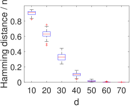
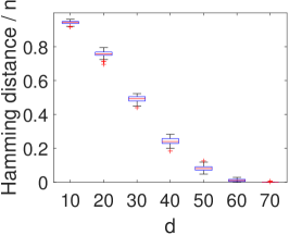
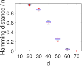
Figure 3: Boxplots of the scaled Hamming distance $\frac{1}{n}\sum_{i=1}^{n}\mathbb{I}(\widehat{\pi}(i)\neq\pi^{*}(i))$ between $\widehat{\pi}$ (from (13)) and the ground truth $\pi^{*}$ based on 100 replications for each setting (plot) and each value of $d$ (horizontal axis).

4.2 Denoising, $d=1$

In this subsection, we compare the performance of the proposed approach with regard to denoising (T2) to two methods proposed in earlier work [32, 4]. These two competing methods only discuss the case $d=1$, hence our comparison is confined to this case. For our comparison, we adopt the five settings for the function $f^{*}$ considered in [4] and depicted in the left panel of Figure 4. Specifically, these five setting are given by

• linear: $f^{*}(x)=x$, $x\in[0,10]$,

• constant: $f^{*}(x)=0$, $x\in[0,10]$,

• step2: $f^{*}(x)=2\mathbb{I}(x\in[0,5))+8\mathbb{I}(x\in[0,10])$,

• step3: $f^{*}(x)=5\mathbb{I}(x\in[10/3,20/3))+10\mathbb{I}(x\in[20/3,10])$,

• power: $f^{*}(x)=-(x-5)^{4}\mathbb{I}(x\in(0,5])+(x-5)^{4}\mathbb{I}(x\in[5,10])$.

The design points $\{X_{i}\}_{i=1}^{n}$ are sampled i.i.d. uniformly from the interval $[0,10]$, and $Y_{i}=f^{*}(X_{i})+\epsilon_{i}$, $1\leq i\leq n$ (without loss of generality, we choose the permutation $\pi^{*}$ as the identity). For the errors, we consider both Gaussian noise with zero mean and unit variance as well as Laplacian noise with zero mean and scale parameter equal to one. We consider $n=100$ and $n=1000$; comparison for larger $n$ were not considered since the approach in [4] does not scale favorably with $n$, incurring a runtime complexity of $O(n^{2})$ per gradient iteration. Hundred independent replications are performed for each configuration in terms of the setting for $f^{*}$, noise distribution, and sample size.

The proposed approach (Slawski & Sen, short SS) is run by solving the approximate NPMLE problem (10) with $\mathbb{G}$ chosen as a linearly spaced grid of size $2\lceil n^{1/2}\rceil$ between $\min_{i}Y_{i}$ and $\max_{i}Y_{i}$, and the resulting deconvolution estimate $\widehat{\nu}=\sum_{j=1}^{p}\widehat{\alpha}_{j}\delta_{\widehat{\theta}_{j}}$ is used for the Kantorovich problem (12). The competitor BDD (initials of the last names of the authors of [4]) is run based on an in-house implementation of the gradient descent method in that paper, using the starting values $\widehat{f}(X_{(i)})=Y_{(i)}$, $1\leq i\leq n$. Gradient descent is performed with constant step size; for the sake of fair comparison, six different values for the step size between $0.01$ and $0.5$ are considered, and for each configuration we report the result of the specific step size achieving minimum average error over the respective replications. The competitor RW (Rigollet & Weed, [32]) is run based on an in-house implementation of a subgradient descent method to solve the (discretized) Wasserstein deconvolution problem considered in that paper (cf. $\S$2.2 therein). The size of the quantization alphabet is taken as $\lceil 2\sqrt{n}\rceil$, linearly spaced between $\min_{i}Y_{i}$ and $\max_{i}Y_{i}$. Each optimal transport problem required for subgradient computation is approximated via Sinkhorn’s algorithm [33, $\S$4] with regularization parameter $\varepsilon=0.1$. As for BDD, we consider six different values for the step size between $5\cdot 10^{-5}$ and $2\cdot 10^{-3}$, and select the results achieving minimum average error over these six choices. Results. The results of our comparison are visualized in Figure 4 via boxplots showing the mean squared denoising errors over 100 replications. The general picture is that BDD achieves the best empirical performance (with optimized step size), while the performance of the proposed approach SS is often on par with BDD. In our comparison, the relative performance of SS is worse for “smooth” $f^{*}$ (settings linear and power). By contrast, RW performs rather poorly for the settings constant, step2, and step3. Somewhat surprisingly, RW does not exhibit any noticeable decrease in error as the sample size is increased from $100$ to $1000$ with the exception of setting linear and Gaussian errors. Despite careful monitoring of convergence and inspection of potential computational issues, it is quite well possible that the performance of RW can be improved substantially with a refined implementation since in fact all three approaches compared herein follow rather similar rationales, and gaps in performance are thus not expected.

$\begin{array}[]{c}\\[-12.91663pt] \includegraphics[height=60.70432pt]{plots/comparison_univariate_setting_1.pdf}\end{array}$	$\begin{array}[]{l}\hskip 34.44434pt\text{Gaussian errors}\\ \includegraphics[height=80.94424pt]{plots/comparison_univariate_g_1.pdf}\end{array}$	$\begin{array}[]{l}\hskip 34.44434pt\text{Laplace errors}\\ \includegraphics[height=80.94424pt]{plots/comparison_univariate_la_1.pdf}\end{array}$
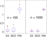
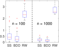
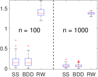
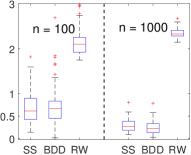
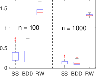
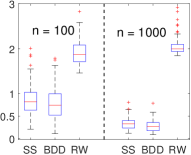
$\begin{array}[]{c}\\[-120.55518pt] \includegraphics[height=60.70432pt]{plots/comparison_univariate_setting_2.pdf}\end{array}$
$\begin{array}[]{c}\\[-120.55518pt] \includegraphics[height=60.70432pt]{plots/comparison_univariate_setting_3.pdf}\end{array}$
$\begin{array}[]{c}\\[-120.55518pt] \includegraphics[height=60.70432pt]{plots/comparison_univariate_setting_4.pdf}\end{array}$
$\begin{array}[]{c}\\[-120.55518pt] \includegraphics[height=60.70432pt]{plots/comparison_univariate_setting_5.pdf}\end{array}$

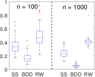
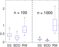
Figure 4: Results of the comparison of the three approaches under consideration for the denoising problem (T2). Left: underlying function $f^{*}$. Middle and right: Boxplots of mean squared errors for Gaussian and Laplace errors, respectively.

4.3 Denoising, $d>1$

This subsection is intended to corroborate and complement aspects of our theoretical results in $\S$3.2 regarding task (T2) for general dimension. The competitors in the preceding section were developed for the case $d=1$, hence we confine ourselves to the proposed method.

We generate data following the permuted regression setup (1). The sample $\{X_{i}\}_{i=1}^{n}$ is sampled uniformly from the unit Euclidean ball in $\mathbb{R}^{d}$ ($d=2,4$), and subsequently we generate $Y_{i}=f^{*}(X_{i})+\sigma\epsilon_{i}$, $1\leq i\leq n$, where $\sigma=1/16$ and the $\{\epsilon_{i}\}_{i=1}^{n}$ are sampled i.i.d. from the $N(0,I_{d})$-distribution and alternatively from the multivariate Laplace distribution. The settings considered for $f^{*}$ are summarized in Table 1. For the sample size, we consider $n=2^{8},2^{9},\ldots,2^{12}=4096$ (and in some selected settings $2^{13}$) in anticipation of slow rates as indicated by the results in $\S$3.2.

The proposed approach is run as follows: we solve the approximate NPMLE problem (11) with $\mathbb{G}=\{Y_{i}\}_{i=1}^{n}$ equipped with knowledge of $\varphi_{\sigma}$, and use the resulting deconvolution estimate $\widehat{\nu}$ in the Kantorovich problem (12) to obtain $\{\widehat{f}(X_{i})\}_{i=1}^{n}$. We then report the normalized MSE $\frac{1}{n\sigma^{2}}\sum_{i=1}^{n}\lVert\widehat{f}(X_{i})-f^{*}(X_{i})\rVert_{2}^{2}$. The results depicted in Figure 5 represent averages over 100 independent replications, with bars indicating $\pm$ standard error.

	cluster	linear	separable	sphere	radial
$\psi_{f^{*}}(x)$	$\max\limits_{1\leq j\leq k}\langle a_{j},x\rangle$	$\frac{1}{2}x^{\top}\sum_{j=1}^{k}v_{j}v_{j}^{\top}x$	$\frac{2}{3}\sum_{j=1}^{d}(x_{j}+1)^{3/2}$	$\lVert x\rVert_{2}$	$\exp(\lVert x\rVert_{2}^{2}/2)$
$f^{*}(x)$	$a_{x}$	$\sum_{j=1}^{k}\langle x,v_{j}\rangle v_{j}$	$\sum_{j=1}^{d}(x_{j}+1)^{1/2}$	$\frac{x}{\lVert x\rVert_{2}}$	$x\cdot\exp(\lVert x\rVert_{2}^{2}/2)$

Table 1: Summary of the simulation settings considered in $\S$4.3. In the 2nd column from the left, $a_{x}$ is short for $\{a_{j}:\left\langle x,a_{j}\right\rangle=\psi_{f^{*}}(x)\}$.

Results. First, the results shown in Figure 5 confirm that the rates are indeed slow as expected in light of the results in $\S$3.2, with an error decay that is linear on a log-log scale for some instances (corresponding to a polynomial rate in $n$) and noticeably sublinear for others. While the discussion at the end of $\S$3.2 suggests that Laplacian errors will yield faster rates, this is not confirmed by our simulations; the observed denoising error is often comparable if not higher than for Gaussian errors. Moreover, while the analysis in $\S$3.2 requires strong convexity of $\psi_{f^{*}}$, several of the settings considered here (cluster, linear with $k<d$ and sphere) do not comply with that assumption, yet the empirical results shown here do not indicate that the lack of strong convexity prompts a substantially different scaling of the denoising error. In fact, the setting cluster corresponds to a clustering problem with a finite number of clusters, i.e., the underlying problem is parametric rather than non-parametric, and one would hence intuitively expect even faster rates (this intuition is confirmed by our results). In a similar vein, we also observe smaller errors if the “intrinsic dimension” of the problem is smaller than the ambient dimension: in the setting linear, the parameter $k$ reflects the intrinsic dimension, and Figure 5 indeed shows that the denoising error drops as $k$ is reduced. For several settings with $d=4$ (in particular sphere and radial) the denoising error is essentially flat and starts decreasing only after $n$ becomes rather large. This behavior is not understood at this point; one possible explanation for the setting sphere might be the lack of strong convexity in conjunction with the absence of additional structure such as in the setting cluster.

$\begin{array}[]{l}\hskip 25.83325pt\text{{clusters}, $d=2$}\\ \includegraphics[width=138.76157pt]{plots/clusters_2}\end{array}$	$\begin{array}[]{l}\hskip 38.74988pt\text{{linear}, $d=2$}\\ \includegraphics[width=138.76157pt]{plots/linear_2}\end{array}$	$\begin{array}[]{l}\hskip 38.74988pt\text{{separable}}\\ \includegraphics[width=138.76157pt]{plots/separable}\end{array}$
$\begin{array}[]{l}\hskip 21.52771pt\text{{clusters}, Laplace, $d=2$}\\ \includegraphics[width=138.76157pt]{plots/clusters_laplace_2}\end{array}$	$\begin{array}[]{l}\hskip 30.1388pt\text{{linear}, Laplace, $d=2$}\\ \includegraphics[width=138.76157pt]{plots/linear_2_laplace}\end{array}$	$\begin{array}[]{l}\hskip 38.74988pt\text{{separable}, Laplace}\\ \includegraphics[width=138.76157pt]{plots/separable_laplace}\end{array}$
$\begin{array}[]{l}\hskip 34.44434pt\text{{clusters}, $d=4$}\\ \includegraphics[width=138.76157pt]{plots/clusters_4}\end{array}$	$\begin{array}[]{l}\hskip 38.74988pt\text{{linear}, $d=4$}\\ \includegraphics[width=138.76157pt]{plots/linear_4}\end{array}$	$\begin{array}[]{l}\hskip 38.74988pt\text{{sphere}}\\ \includegraphics[width=138.76157pt]{plots/sphere}\end{array}$
$\begin{array}[]{l}\hskip 21.52771pt\text{{clusters}, Laplace, $d=4$}\\ \includegraphics[width=138.76157pt]{plots/clusters_laplace_4}\end{array}$	$\begin{array}[]{l}\hskip 30.1388pt\text{{linear}, Laplace, $d=4$}\\ \includegraphics[width=138.76157pt]{plots/linear_4_laplace}\end{array}$	$\begin{array}[]{l}\hskip 38.74988pt\text{{sphere}, Laplace}\\ \includegraphics[width=138.76157pt]{plots/sphere_laplace.pdf}\end{array}$
	$\begin{array}[]{l}\hskip 38.74988pt\text{{radial}}\\ \includegraphics[width=138.76157pt]{plots/radial.pdf}\end{array}$	$\begin{array}[]{l}\hskip 38.74988pt\text{{radial}, Laplace}\\ \includegraphics[width=138.76157pt]{plots/radial_laplace.pdf}\end{array}$

Figure 5: Denoising results for $d=2,4$; “MSE” refers to $\frac{1}{n\sigma^{2}}\sum_{i=1}^{n}\lVert\widehat{f}(X_{i})-f^{*}(X_{i})\rVert_{2}^{2}$. The results shown represent averages $\pm$1 standard error (the error bars are hardly visible for most instances) over 100 independent replications for the respective setting given in the plot captions (unless specified otherwise, the noise distribution is Gaussian).

5 Conclusion

In this paper, we have considered permuted and uncoupled regression for maps $f^{*}:\mathbb{R}^{d}\rightarrow\mathbb{R}^{d}$ that are gradients of convex functions, the multi-dimensional analog of isotonic functions. This paper has studied exact permutation recovery and denoising, and has established several connections to several recent works involving related permuted data problems. The task of denoising is tackled via deconvolution based on the Kiefer-Wolfowitz NPMLE and optimal transport. The rich literature and the recently surging interest regarding the latter topic facilitates the analysis of the proposed approach. Compared to prior work on one-dimensional permuted regression problems, the implementation of our approach is particularly convenient since the underlying convex optimization problems are straightforward to solve and require almost no tuning; currently, the only parameter to be specified is the grid for the approximate Kiefer-Wolfowitz problem, for which straightforward default options are available that yield reasonable results empirically (cf. $\S$4).

Despite the advances made in the current paper, there are several open problems and possible extensions from both practical and theoretical viewpoints as discussed below. (I)Towards deconvolution with unknown distribution of the errors. Even though this objective appears not to be achievable in general, it is of great practical importance to relax the somewhat unrealistic assumption that the distribution of the error terms is fully known. As first steps, the following directions can be pursued: (i) the scale parameter $\sigma$ is not known, and needs to be selected in a data-driven manner, and (ii) the model used for the errors is (mildly) misspecified. (II) Beyond denoising. In this paper, we only consider denoising, i.e., the estimation of the values of the unknown function $f^{*}$ at the sample points $\{X_{i}\}_{i=1}^{n}$. A next step is to develop an approach that provides a (smooth) estimate of $f^{*}$ over, say, a compact domain. (III) Minimaxity, adaptation, strong convexity. Concerning our results obtained for denoising, the minimax rate is yet unknown except for $d=1$ [32]. While slow rates appear inevitable in general, parts of our simulation results indicate that faster rates can be obtained for instances with additional structure such as piecewise affine functions and functions with low intrinsic dimensionality. In this context, it is of interest to study whether the proposed approach adapts to such underlying low-complexity structure. Moreover, our results currently hinge on strong convexity, and it merits further investigation whether this assumption can be relaxed. (IV) Wasserstein vs. maximum likelihood (ML) deconvolution. The approach presented in this paper is based on the Kiefer-Wolfowitz problem and thus ML deconvolution. Our analysis, however, is based on bounding the distance to the underlying mixing measure in Wasserstein distance. This raises the question whether the use of the Wasserstein distance (as done in [32] for $d=1$) instead of the Kullback-Leibler divergence is more suitable for the problem at hand. At the same time, ML deconvolution is considerably more convenient from a computational perspective. An interesting connection between ML deconvolution and entropic optimal transport is made in [70]. It is of interest to study whether that connection can be leveraged to facilitate the analysis of the proposed approach. (V) Beyond equal dimensions. The route taken in this paper requires $f^{*}$ to be a map from $\mathbb{R}^{d}$ to $\mathbb{R}^{d}$. This requirement can be limiting in applications in which the two samples $\mathcal{X}_{n}$ and $\mathcal{Y}_{n}$ live in different dimensions.

Appendix A Proofs of main results

This appendix contains proofs of our main results and additional technical background and discussion. The proofs of Theorems 2, 3 and Proposition 3 are decomposed into several key pieces which are presented in dedicated sections. The specific constituents and their dependencies are outlined in Figure 6.

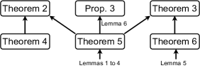
Figure 6: Chart summarizing the organization of the proofs of our main results on denoising (T2).

A.1 Proof of Proposition 2

Without loss of generality, we may assume that $\pi^{*}$ is the identity permutation, i.e., $\pi^{*}(i)=i$, $1\leq i\leq n$. It then suffices to show that the set $\{(X_{i},Y_{i})\}_{i=1}^{n}$ is cyclically monotone with respect to the cost function $c_{0}(x,y):=\lVert x-y\rVert_{2}^{2}$, or equivalently the cost function $c(x,y)=-\left\langle x,y\right\rangle$, under the conditions stated in the proposition. For this purpose, we need to show that for any subset $\{(X_{i_{j}},Y_{i_{j}})\}_{j=1}^{k}$ of $\{(X_{i},Y_{i})\}_{i=1}^{n}$ of size $k\geq 2$, it holds that

$$-\sum_{j=1}^{k}\left\langle X_{i_{j}},Y_{i_{j}}\right\rangle\leq-\sum_{j=1}^{k}\left\langle X_{i_{j+1}},Y_{i_{j}}\right\rangle,\quad i_{k+1}=i_{1}.$$ (20)

Expanding $Y_{i_{j}}=f^{*}(X_{i_{j}})+\epsilon_{i_{j}}$, $1\leq j\leq k+1$, the above inequality becomes

$$-\sum_{j=1}^{k}\left\langle X_{i_{j}},f^{*}(X_{i_{j}})+\epsilon_{i_{j}}\right\rangle\leq-\sum_{j=1}^{k}\left\langle X_{i_{j+1}},f^{*}(X_{i_{j}})+\epsilon_{i_{j}}\right\rangle.$$

Re-arranging in order to single out the contributions of the noise yields the following condition equivalent to (20)

$$\sum_{j=1}^{k}\left\langle X_{i_{j+1}}-X_{i_{j}},f^{*}(X_{i_{j}})\right\rangle+\sum_{j=1}^{k}\left\langle X_{i_{j+1}}-X_{i_{j}},\epsilon_{i_{j}}\right\rangle\leq 0.$$ (21)

By $\lambda$-strong convexity of $\psi_{f^{*}}$, we have

$$\psi_{f^{*}}(X_{i_{j+1}})-\psi_{f^{*}}(X_{i_{j}})-\langle\underbrace{\nabla\psi_{f^{*}}(X_{i_{j}})}_{f^{*}(X_{i_{j}})},X_{i_{j+1}}-X_{i_{j}}\rangle\geq\lambda\lVert X_{i_{j+1}}-X_{i_{j}}\rVert_{2}^{2},\quad 1\leq j\leq k.$$

Summation of the above inequality over $j$ and using the cyclicity condition $i_{k+1}=i_{1}$ yields

$$\sum_{j=1}^{k}\left\langle X_{i_{j+1}}-X_{i_{j}},f^{*}(X_{i_{j}})\right\rangle\leq-\lambda\sum_{j=1}^{k}\lVert X_{i_{j+1}}-X_{i_{j}}\rVert_{2}^{2}.$$ (22)

We now upper bound the second term in (21). Conditional on the $\{X_{i}\}_{i=1}^{n}$ and using the independence of the errors, we have

$$\sum_{j=1}^{k}\left\langle X_{i_{j+1}}-X_{i_{j}},\epsilon_{i_{j}}\right\rangle\sim N\Big{(}0,\sigma^{2}\sum_{j=1}^{k}\lVert X_{i_{j+1}}-X_{i_{j}}\rVert_{2}^{2}\Big{)}.$$

Now define the quantity

$$M_{k}:=\max_{\{i_{1},\ldots,i_{k}\}\subseteq\{1,\ldots,n\}}\frac{1}{\sqrt{\sum_{j=1}^{k}\lVert X_{i_{j+1}}-X_{i_{j}}\rVert_{2}^{2}}}\sum_{j=1}^{k}\left\langle X_{i_{j+1}}-X_{i_{j}},\epsilon_{i_{j}}\right\rangle.$$ (23)

The standard Gaussian tail bound $\operatorname{\mathbf{P}}(Z>z)\leq\exp(-z^{2}/2)$ for $z\geq 0$, $Z\sim N(0,1)$, combined with the union bound and the inequality $\binom{n}{k}\leq\left(\frac{en}{k}\right)^{k}$ yields

$$\operatorname{\mathbf{P}}(M_{k}\geq t)\leq\exp\left(-\frac{t^{2}}{2\sigma^{2}}+k\log(en/k)\right).$$

Choosing $t=\sigma\sqrt{4\log n+2k\log(en/k)}$, we obtain that

$$\operatorname{\mathbf{P}}\left(M_{k}\geq\sigma\sqrt{4\log n+2k\log(en/k)}\right)\leq\frac{1}{n^{2}}.$$ (24)

Combining (21), (22), (23), we note that the desired condition (20) is implied by the condition

$$\forall k=2,\ldots,n:\quad\lambda\sqrt{k}\min_{i<j}\lVert X_{i}-X_{j}\rVert\geq M_{k}.$$

Using (24) along with the observation that the function $k\mapsto\sigma\sqrt{4\log(n)/k+2\log(en/k)}$ is decreasing in $k$, a union bound over $k=2,\ldots,n$, yields that if

$$\min_{i<j}\lVert X_{i}-X_{j}\rVert_{2}\geq\frac{\sigma\sqrt{6\log n}}{\lambda},$$

the required inequality (20) for cyclic monotonicity holds with probability at least $1-1/n$.

Appendix B Proof of Theorems 2 and 3 and Proposition 3

The proofs of these two theorems involve a few other results, which we first state in the following subsections. These results may be of independent interest.

Let $\nu_{n}^{*}:=\frac{1}{n}\sum_{i=1}^{n}\delta_{\theta_{i}^{*}}=\frac{1}{n}\sum_{i=1}^{n}\delta_{f^{*}(X_{i})}$, and let $\widehat{\nu}$ denote the mixing measure associated with the NPMLE (9). Theorem 4 below provides an upper bound on the empirical $L_{2}$-loss of the barycentric projection estimator $\{\widehat{f}(X_{i})\}_{i=1}^{n}$, obtained from an optimal coupling between $\nu_{n}^{*}$ and $\widehat{\nu}$ (see (8)), in terms of the 2-Wasserstein distance between $\nu_{n}^{*}$ and $\widehat{\nu}$.

B.1 Analysis of the Kantorovich problem (12) for general $d$

The result below is the central technical component in proving Theorem 2; see Appendix C.1 for its proof.

Theorem 4.

Consider the atomic measure $\nu_{n}^{*}:=\frac{1}{n}\sum_{i=1}^{n}\delta_{\theta_{i}^{*}}$, $\theta_{i}^{*}=f^{*}(X_{i})$, $1\leq i\leq n$, with $f^{*}=\nabla\psi_{f^{*}}$ such that assumptions (A1) through (A3) in $\S$3.2 are satisfied, and let $\widehat{\nu}:=\sum_{j=1}^{p}\widehat{\alpha}_{j}\delta_{\widehat{\theta}_{j}}$ be another atomic measure on $\mathbb{R}^{d}$. Let further $\mu_{n}:=\frac{1}{n}\sum_{i=1}^{n}\delta_{X_{i}}$, and consider the barycentric projection (8) based on an optimal coupling (7) between $\mu_{n}$ and $\widehat{\nu}$. We then have

$$\frac{1}{n}\sum_{i=1}^{n}\lVert\widehat{f}(X_{i})-f^{*}(X_{i})\rVert_{2}^{2}\leq\frac{L}{\lambda}\emph{\text{$\textsf{W}_{2}^{2}$}}(\nu_{n}^{*},\widehat{\nu}).$$ (25)

We next upper bound $\text{$\textsf{W}_{2}^{2}$}(\nu_{n}^{*},\widehat{\nu})$.

B.2 Wasserstein deconvolution rates

The following result provides an upper bound on the 2-Wasserstein distance between an underlying atomic mixing measure $\nu_{n}^{*}=\frac{1}{n}\sum_{i=1}^{n}\delta_{\theta_{i}^{*}}$ with uniformly bounded support and a deconvolution estimator $\widehat{\nu}$ in terms of the Hellinger distance between the convolved measures $\nu_{n}^{*}\star\varphi_{\sigma}$ and $\widehat{\nu}\star\varphi_{\sigma}$, along the route of the proof of Theorem 2 in [71]; see Appendix C.3 for a proof.

Theorem 5.

Let $\widehat{\text{\emph{{f}}}}_{n}$ denote the NPMLE (9) with $\varphi(z)=(2\pi)^{-d/2}\exp(-\lVert z\rVert_{2}^{2})$ given $\{Y_{i}\}_{i=1}^{n}\overset{\text{\emph{i.i.d.}}}{\sim}\varphi_{\sigma}\star\nu_{n}^{*}$ with $\nu_{n}^{*}=\frac{1}{n}\sum_{i=1}^{n}\delta_{\theta_{i}^{*}}$ such that $\{\theta_{i}^{*}\}_{i=1}^{n}$ is contained in a Euclidean ball of radius $B$ centered at the origin, and let $\widehat{\nu}$ be the mixing measure associated with the NPMLE, i.e., $\widehat{\nu}\star\varphi_{\sigma}=\widehat{\text{\emph{{f}}}}_{n}$. Choose $s>k\geq 1$, and suppose that $n\geq C_{0}(d,B,\sigma)(\log n)^{d+1}$. It then holds with probability at least $1-5/n$,

$$\text{\emph{$\textsf{W}_{k}^{k}$}}(\nu_{n}^{*},\widehat{\nu})\leq C(s,k,d,\sigma,B)\left(\frac{1}{\log n}\right)^{k/2},$$

where $C_{0}$ and $C$ are positive constants depending only on the quantities in the parentheses.

B.3 Analysis of the Kantorovich problem (12) for general $d$ when $m\neq n$

The next result (proved in Appendix C.2) extends Theorem 4 to the unlinked setting based on samples $\mathcal{X}_{n}=\{X_{1},\ldots,X_{n}\}$ and $\mathcal{Y}_{m}=\{Y_{1},\ldots,Y_{m}\}$. The proof requires only one additional ingredient (Lemma 5) to the preceding proof.

Theorem 6.

Let $X_{1},\ldots,X_{n}\overset{\text{\emph{i.i.d.}}}{\sim}\mu$ and $\theta_{1}^{*},\ldots,\theta_{m}^{*}\overset{\text{\emph{i.i.d.}}}{\sim}\nu$, where the support of $\nu$ is contained in a Euclidean ball of radius $B$, and let $f^{*}=\nabla\psi_{f^{*}}$ be the Brenier map (cf. Theorem 7) transporting $\mu$ to $\nu$ with $f^{*}$ satisfying (A1) and (A2). Consider the atomic measures $\nu_{n}^{*}=\frac{1}{n}\sum_{i=1}^{n}\delta_{f^{*}(X_{i})}$, $\nu_{m}^{*}=\frac{1}{m}\sum_{i=1}^{m}\delta_{\theta_{i}^{*}}$, and $\widehat{\nu}=\sum_{j=1}^{p}\widehat{\alpha}_{j}\delta_{\widehat{\theta}_{j}}$.

Let further $\mu_{n}=\frac{1}{n}\sum_{i=1}^{n}\delta_{X_{i}}$, and consider the barycentric projection (8) based on an optimal coupling (7) between $\mu_{n}$ and $\widehat{\nu}$. For positive constants $C,c>0$, we then have, with probability at least $1-C(n^{-c}+m^{-c})$,

$$\frac{1}{n}\sum_{i=1}^{n}\lVert\widehat{f}(X_{i})-f^{*}(X_{i})\rVert_{2}^{2} \leq\frac{2L}{\lambda}\Bigg{(}\emph{\text{$\textsf{W}$}}_{2}^{2}(\widehat{\nu},\nu_{m}^{*})+2\sqrt{\frac{\log n}{n}}\vee\Big{(}\frac{\log n}{n}\Big{)}^{2/d}+2\sqrt{\frac{\log m}{m}}\vee\Big{(}\frac{\log m}{m}\Big{)}^{2/d}\Bigg{)}.$$

B.4 Proof of Theorem 2

Recall that $\nu_{n}^{*}=\frac{1}{n}\sum_{i=1}^{n}\delta_{\theta_{i}^{*}}=\frac{1}{n}\sum_{i=1}^{n}\delta_{f^{*}(X_{i})}$, and note that $\widehat{\nu}$ denotes the mixing measure associated with the NPMLE (9). Theorem 4 above then yields that the barycentric projection estimator $\{\widehat{f}(X_{i})\}_{i=1}^{n}$, obtained from an optimal coupling between $\nu_{n}^{*}$ and $\widehat{\nu}$ (see (8)), obeys the bound (25).

Next, note that, under the stated condition on $n$, the squared 2-Wasserstein distance between $\nu_{n}^{*}$ and $\widehat{\nu}$ can be bounded as $\textsf{W}_{2}^{2}(\nu_{n}^{*},\widehat{\nu})\lesssim_{d,\sigma,B}\frac{1}{\log n}$ according to Theorem 5 with the stated probability. This completes the proof of the theorem. ∎

B.5 Proof of Theorem 3

The main modification relative to the previous proof is to consider both $\nu_{n}^{*}:=\frac{1}{n}\sum_{i=1}^{n}\delta_{f^{*}(X_{i})}$ and $\nu_{m}^{*}:=\frac{1}{m}\sum_{i=1}^{m}\delta_{\theta_{i}^{*}}$, where $\{\theta_{i}^{*}\}_{i=1}^{m}\overset{\text{i.i.d.}}{\sim}\nu$. Theorem 6 bounds the mean squared denoising error in terms of the Wasserstein distance $\textsf{W}_{2}^{2}(\nu_{m}^{*},\widehat{\nu})$ and additional lower-order terms, where $\widehat{\nu}$ denotes the mixing measure associated with the NPMLE (9) based on the sample $\{Y_{i}\}_{i=1}^{m}$. We finally invoke Theorem 5 to bound $\textsf{W}_{2}^{2}(\nu_{m}^{*},\widehat{\nu})$, with $\nu_{n}^{*}$ and $\{\theta_{i}^{*}\}_{i=1}^{n}$ replaced by $\nu_{m}^{*}$ and $\{\theta_{i}^{*}\}_{i=1}^{m}$, respectively. ∎

B.6 Proof of Proposition 3

Let us consider the permuted regression setup (1), and consider the two Kantorovich problems

$$\text{(i)}\;\min_{\gamma\in\Pi(\mu_{n},\widehat{\nu})}\int(x-\theta)^{2}\,d\gamma(x,\theta),\qquad\text{(ii)}\;\min_{\gamma\in\Pi(\nu_{n}^{*},\widehat{\nu})}\int(\zeta-\theta)^{2}\,d\gamma(\zeta,\theta).$$

Let $\widehat{\gamma}^{1}$ denote the so-called Northwest-corner solution of (i), cf. [33, $\S$3.4.2], and let $\widetilde{\gamma}^{1}=(f^{*},\textsf{id})\#\widehat{\gamma}^{1}$ the push-forward (cf. Definition 1 in Appendix G) of $\widehat{\gamma}^{1}$ under the transformation that pushes forward its two marginals to $f^{*}\#\mu_{n}=\nu_{n}^{*}$ and and $\textsf{id}\#\widehat{\nu}=\widehat{\nu}$, where id denotes the identity map. Since the $\{X_{i}\}_{i=1}^{n}$ and $\{\theta_{i}^{*}\}_{i=1}^{n}$ associated with $\mu_{n}$ and $\nu_{n}^{*}$ are related by the non-decreasing transformation $f^{*}$, $\widetilde{\gamma}^{1}$ is a minimizer of (ii) as follows, e.g., from Proposition 1 in [50]. Consequently, letting $\widetilde{\theta}_{i}=\operatorname{\mathbf{E}}_{(\theta,\zeta)\sim\widetilde{\gamma}^{1}}[\theta|\zeta=\theta_{i}^{*}]$, $1\leq i\leq n$, denote the barycentric projections, we have

$$\widetilde{\theta}_{i}=\frac{\int_{\theta}\theta\;d\widetilde{\gamma}^{1}(\theta_{i}^{*},\theta)}{\int_{\theta}\;d\widetilde{\gamma}^{1}(\theta_{i}^{*},\theta)}=\frac{\int_{\theta}\theta\;d\widehat{\gamma}^{1}(X_{i},\theta)}{\int_{\theta}\;d\widehat{\gamma}^{1}(X_{i},\theta)}=\widehat{f}(X_{i}),\quad 1\leq i\leq n,$$

where the last equality is simply the definition of the $\{\widehat{f}(X_{i})\}_{i=1}^{n}$ (cf. (8)). On the other hand, by Lemma 6, $\frac{1}{n}\sum_{i=1}^{n}(\widetilde{\theta}_{i}-\theta_{i}^{*})^{2}\leq\textsf{W}_{2}^{2}(\nu_{n}^{*},\widehat{\nu})$, which concludes the proof.

The proof for the uncoupled regression setup is analogous to the proof of Theorem 3 (cf. Theorem 6 and its proof) and is hence omitted. ∎

Appendix C Proof of Theorems 4, 5 and 6

C.1 Proof of Theorem 4

Proof.

Consider an optimal coupling $\widehat{\gamma}$ between $\widehat{\nu}$ and $\mu_{n}$ minimizing (7), and let $\widehat{\gamma}_{ij}$ denote the resulting probability mass that is assigned to $X_{i}$ and $\widehat{\theta}_{j}$, $1\leq i\leq n$, $1\leq j\leq p$. Define further $\pi_{j}(X_{i})=\widehat{\Gamma}_{ij}n$, $1\leq i\leq n$, $1\leq j\leq p$. Accordingly, we have $\widehat{\alpha}_{j}=\frac{1}{n}\sum_{i=1}^{n}\pi_{j}(X_{i})=\int\pi_{j}(x)\;d\mu_{n}(x)$, $1\leq j\leq p$. Recall that $\psi_{f^{*}}^{\star}$ denotes the Legendre-Fenchel conjugate of $\psi_{f^{*}}$. We first bound $\int\psi_{f^{*}}^{\star}(\theta)\;d\widehat{\nu}(\theta)-\int\psi_{f^{*}}^{\star}(\theta)\;d\nu_{n}^{*}(\theta)$ as

$$\sum_{j=1}^{p}\psi_{f^{*}}^{\star}(\widehat{\theta}_{j})\widehat{\alpha}_{j}-\int\psi_{f^{*}}^{\star}(\theta)\;d\nu_{n}^{*}(\theta)$$

$$= \int\sum_{j=1}^{p}\pi_{j}(x)\psi_{f^{*}}^{\star}(\widehat{\theta}_{j})\;d\mu_{n}(x)-\int\psi_{f^{*}}^{\star}(f^{*}(x))\;d\mu_{n}(x)$$

$$\geq \int\psi_{f^{*}}^{\star}\left(\sum_{j=1}^{p}\pi_{j}(x)\widehat{\theta}_{j}\right)\;d\mu_{n}(x)-\int\psi_{f^{*}}^{\star}(f^{*}(x))\;d\mu_{n}(x)$$

$$= \int\psi_{f^{*}}^{\star}(\widehat{f}(x))\;d\mu_{n}(x)-\int\psi_{f^{*}}^{\star}(f^{*}(x))\;d\mu_{n}(x)$$

$$\geq \int\nabla\psi_{f^{*}}^{\star}(f^{*}(x))^{\top}(\widehat{f}(x)-f^{*}(x))\;d\mu_{n}(x)\;+\frac{1}{2L}\int\lVert\widehat{f}(x)-f^{*}(x)\rVert_{2}^{2}\;d\mu_{n}(x),$$

$$= \int x^{\top}(\widehat{f}(x)-f^{*}(x))\;d\mu_{n}(x)+\frac{1}{2L}\int\lVert\widehat{f}(x)-f^{*}(x)\rVert_{2}^{2}\;d\mu_{n}(x)$$ (26)

where the two inequalities follow from convexity and $L$-smoothness of $\psi_{f^{*}}$ in virtue of (A2), which implies $\frac{1}{L}$-strong convexity of its conjugate $\psi_{f^{*}}^{\star}$ [72]; the last equality follows from Brenier’s theorem (Theorem 7 in Appendix G) in light of which $\nabla\psi_{f^{*}}^{\star}$ is the inverse map of $f^{*}=\nabla\psi_{f^{*}}$. Moreover, the squared 2-Wasserstein distance between $\widehat{\nu}$ and $\mu_{n}$, i.e., $\textsf{W}_{2}^{2}(\widehat{\nu},\mu_{n})$, can be expressed as

$$\sum_{i=1}^{n}\sum_{j=1}^{p}\lVert\widehat{\theta}_{j}-X_{i}\rVert_{2}^{2}\widehat{\Gamma}_{ij} =\sum_{j=1}^{p}\widehat{\alpha}_{j}\lVert\widehat{\theta}_{j}\rVert_{2}^{2}+\frac{1}{n}\sum_{i=1}^{n}\lVert X_{i}\rVert_{2}^{2}-2\sum_{i=1}^{n}\sum_{j=1}^{p}\langle\widehat{\theta}_{j},X_{i}\rangle\widehat{\Gamma}_{ij}$$

$$=\int\lVert\theta\rVert_{2}^{2}\;d\widehat{\nu}(\theta)+\int\lVert x\rVert_{2}^{2}\;d\mu_{n}(x)-\frac{2}{n}\sum_{i=1}^{n}\left\langle X_{i},\sum_{j=1}^{p}n\widehat{\Gamma}_{ij}\widehat{\theta}_{j}\right\rangle$$

$$=\int\lVert\theta\rVert_{2}^{2}\;d\widehat{\nu}(\theta)+\int\lVert x\rVert_{2}^{2}\;d\mu_{n}(x)-2\int x^{\top}\widehat{f}(x)\;d\mu_{n}(x).$$ (27)

Similarly,

$$\textsf{W}_{2}^{2}(\nu_{n}^{*},\mu_{n})=\int\lVert\theta\rVert_{2}^{2}\;d\nu_{n}^{*}(\theta)+\int\lVert x\rVert_{2}^{2}\;d\mu_{n}(x)-2\int x^{\top}f^{*}(x)\;d\mu_{n}(x)$$ (28)

where we note that $f^{*}$ is the optimal transport map from $\nu_{n}^{*}$ to $\mu_{n}$ (as $f^{*}\#\mu_{n}=\nu_{n}^{*}$ and $f^{*}$ is the gradient of a convex function). Combining (26), (27), (28), we obtain that

$$\int\lVert\widehat{f}(x)-f^{*}(x)\rVert_{2}^{2}\;d\mu_{n}(x) \leq L\Big{[}\textsf{W}_{2}^{2}(\widehat{\nu},\mu_{n})-\textsf{W}_{2}^{2}(\nu_{n}^{*},\mu_{n})+2\int\psi_{f^{*}}^{\star}(\theta)\;d(\widehat{\nu}-\nu_{n}^{*})(\theta)$$

$$\qquad+\int\lVert\theta\rVert_{2}^{2}\;d(\nu_{n}^{*}-\widehat{\nu})(\theta)\Big{]}.$$ (29)

Let $\widehat{\eta}$ be an optimal coupling between $\nu_{n}^{*}$ and $\widehat{\nu}$, and let further $\eta=(\nabla\psi_{f^{*}}^{\star},\textsf{id})\#\widehat{\eta}$ be the push-forward (cf. Definition 1) of the coupling $\widehat{\eta}$ under the transformation that pushes forward its two marginals to $\nabla\psi_{f^{*}}^{\star}\#\nu_{n}^{*}=\mu_{n}$ and $\textsf{id}\#\widehat{\nu}=\widehat{\nu}$, where we have used that $\nabla\psi_{f^{*}}^{\star}(\theta_{i}^{*})=X_{i}$, $1\leq i\leq n$, by Brenier’s theorem, with id denoting the identity map.

Accordingly, by the definition of the 2-Wasserstein distance in terms of optimal couplings (cf. Appendix G), we obtain that

$$\textsf{W}_{2}^{2}(\mu_{n},\widehat{\nu})\leq\int\lVert x-\theta\rVert_{2}^{2}\;d\eta(x,\theta)=\int\lVert\nabla\psi_{f^{*}}^{\star}(\zeta)-\theta\rVert_{2}^{2}\;d\widehat{\eta}(\zeta,\theta).$$

Adding and subtracting $\zeta$ inside the norm on the right hand side and expanding the square, it follows that

$$\textsf{W}_{2}^{2}(\mu_{n},\widehat{\nu}) \leq\int\lVert\nabla\psi_{f^{*}}^{\star}(\zeta)-\zeta\rVert_{2}^{2}\,d\nu_{n}^{*}(\zeta)+\int\lVert\theta-\zeta\rVert_{2}^{2}\,d\widehat{\eta}(\zeta,\theta)+2\int\langle\nabla\psi_{f^{*}}^{\star}(\zeta)-\zeta,\zeta-\theta\rangle\,d\widehat{\eta}(\zeta,\theta)$$

$$=\textsf{W}_{2}^{2}(\nu_{n}^{*},\mu_{n})+\textsf{W}_{2}^{2}(\nu_{n}^{*},\widehat{\nu})+2\int\langle\nabla\psi_{f^{*}}^{\star}(\zeta)-\zeta,\zeta-\theta\rangle\,d\widehat{\eta}(\zeta,\theta),$$ (30)

where we have used that $\psi_{f^{*}}^{\star}$ is the optimal transport map pushing forward $\nu_{n}^{*}$ to $\mu_{n}$, the definition of the 2-Wasserstein distance in terms of optimal transport and optimal couplings, and the definition of $\widehat{\eta}$ as optimal coupling between $\nu_{n}^{*}$ and $\widehat{\nu}$.

In order to bound the rightmost term in the preceding display, we invoke (A1) which implies [72] that the function $\psi_{f^{*}}^{\star}$ is $(1/\lambda)$-smooth in the sense of (18). This yields

$$2\int\langle\nabla\psi_{f^{*}}^{\star}(\zeta),\zeta-\theta\rangle\,d\widehat{\eta}(\zeta,\theta) \leq 2\int\left\{\psi_{f^{*}}^{\star}(\zeta)-\psi_{f^{*}}^{\star}(\theta)+\frac{1}{2\lambda}\lVert\zeta-\theta\rVert_{2}^{2}\right\}\,d\widehat{\eta}(\zeta,\theta)$$

$$=2\int\psi_{f^{*}}^{\star}(\zeta)\,d\nu_{n}^{*}(\zeta)-2\int\psi_{f^{*}}^{\star}(\theta)\,d\widehat{\nu}(\theta)+\frac{1}{\lambda}\textsf{W}_{2}^{2}(\nu_{n}^{*},\widehat{\nu}),$$ (31)

using the same argument as for the preceding display to obtain the rightmost term.

Finally, we note that

$$2\int\langle-\zeta,\zeta-\theta\rangle\,d\widehat{\eta}(\zeta,\theta) =\int\left\{\lVert\theta\rVert_{2}^{2}-\lVert\theta-\zeta\rVert_{2}^{2}-\lVert\zeta\rVert_{2}^{2}\right\}\,d\widehat{\eta}(\zeta,\theta)$$

$$=\int\lVert\theta\rVert_{2}^{2}\,d\widehat{\nu}(\theta)-\int\lVert\zeta\rVert_{2}^{2}\,d\nu_{n}^{*}(\zeta)-\textsf{W}_{2}^{2}(\nu_{n}^{*},\widehat{\nu}).$$ (32)

Combining (30), (31), and (32), we obtain that

$$\textsf{W}_{2}^{2}(\mu_{n},\widehat{\nu}) \leq\textsf{W}_{2}^{2}(\nu_{n}^{*},\mu_{n})+\frac{1}{\lambda}\textsf{W}_{2}^{2}(\nu_{n}^{*},\widehat{\nu})+2\int\psi_{f^{*}}^{\star}(\zeta)\,d\nu_{n}^{*}(\zeta)-2\int\psi_{f^{*}}^{\star}(\theta)\,d\widehat{\nu}(\theta)$$

$$\qquad\quad+\int\lVert\theta\rVert_{2}^{2}\,d\widehat{\nu}(\theta)-\int\lVert\zeta\rVert_{2}^{2}\,d\nu_{n}^{*}(\zeta).$$

Substituting this bound back into (29), we observe that all but the term $\frac{L}{\lambda}\textsf{W}_{2}^{2}(\nu_{n}^{*},\widehat{\nu})$ cancel, yielding the assertion of the theorem. ∎

C.2 Proof of Theorem 6

Proof.

We first note that the argument in the previous proof continues to apply with $\nu_{n}^{*}=\frac{1}{n}\sum_{i=1}^{n}\delta_{f^{*}(X_{i})}$, which yields

$$\frac{1}{n}\sum_{i=1}^{n}\lVert\widehat{f}(X_{i})-f^{*}(X_{i})\rVert_{2}^{2}\leq\frac{L}{\lambda}\textsf{W}_{2}^{2}(\widehat{\nu},\nu_{n}^{*})$$

We then use the triangle inequality

$$\textsf{W}_{2}(\widehat{\nu},\nu_{n}^{*})\leq\textsf{W}_{2}(\widehat{\nu},\nu_{m}^{*})+\textsf{W}_{2}(\nu_{m}^{*},\nu_{n}^{*})\leq\textsf{W}_{2}(\widehat{\nu},\nu_{m}^{*})+\textsf{W}_{2}(\nu_{n}^{*},\nu)+\textsf{W}_{2}(\nu_{m}^{*},\nu),$$

and accordingly

$$\textsf{W}_{2}^{2}(\widehat{\nu},\nu_{n}^{*})\leq 2\textsf{W}_{2}^{2}(\widehat{\nu},\nu_{m}^{*})+4(\textsf{W}_{2}^{2}(\nu_{n}^{*},\nu)+\textsf{W}_{2}^{2}(\nu_{m}^{*},\nu)).$$

The proof of the result now follows by invoking Lemma 5 with the choices $t=\sqrt{\log n/n}\vee n^{-2/d}(\log n)^{2/d}$ and $t=\sqrt{\log m/m}\vee m^{-2/d}(\log m)^{2/d}$ to control the second and the third term of the above display, respectively, with the stated probability; for the second term, we use that $\{f^{*}(X_{i})\}_{i=1}^{n}\overset{\text{i.i.d.}}{\sim}\nu$ since $f^{*}$ pushes forward $\mu$ to $\nu$ (cf. Definition 1 and Theorem 7). ∎

C.3 Proof of Theorem 5

Proof.

For a Lebesgue density $h$ on $\mathbb{R}^{d}$ and $q>0$, let $\textsf{M}_{h}^{q}:=\int\lVert x\rVert_{2}^{q}\,h(x)\,dx$ denote the $q$-th moment associated with $h$.

Let $s>k$ be arbitrary and let $K:\mathbb{R}^{d}\rightarrow(0,\infty)$ be a symmetric PDF such that $\textsf{M}_{K}^{s}\mathrel{\mathop{:}}=\int_{\mathbb{R}^{d}}\lVert x\rVert_{2}^{s}\,K(x)\,dx<\infty$ and such that its Fourier transform $\widehat{K}$ is continuous with support contained in $[-1,1]^{d}$, and for $\delta>0$, let $K_{\delta}(\cdot):=\frac{1}{\delta^{d}}K(\cdot/\delta)$. By the triangle inequality, we have

$$\textsf{W}_{k}^{k}(\nu_{n}^{*},\widehat{\nu})\leq 2^{2(k-1)}\left\{\textsf{W}_{k}^{k}(\nu_{n}^{*},\nu_{n}^{*}\star K_{\delta})+\textsf{W}_{k}^{k}(\widehat{\nu},\widehat{\nu}\star K_{\delta})+\textsf{W}_{k}^{k}(\nu_{n}^{*}\star K_{\delta},\widehat{\nu}\star K_{\delta})\right\}.$$ (33)

The first two terms inside the curly brackets are of order $O(\delta^{k})$. To see this, consider couplings defined by the pairs of random variables $(X,X+\epsilon)$ and $(\widehat{X},\widehat{X}+\epsilon)$ with $X\sim\nu_{n}^{*}$, $\widehat{X}\sim\widehat{\nu}$, and $\epsilon$ (independent of ${X}$ and $\widehat{X}$) distributed according to the PDF $K_{\delta}$, and note that $\operatorname{\mathbf{E}}[\lVert X-(X+\epsilon)\rVert^{k}_{2}]=\operatorname{\mathbf{E}}[\lVert\widehat{X}-(\widehat{X}+\epsilon)\rVert^{k}_{2}]=O(\delta^{k})$. In the sequel, the third term $\textsf{W}_{k}^{k}(\nu_{n}^{*}\star K_{\delta},\widehat{\nu}\star K_{\delta})$ will be controlled. By Lemma 3 in Appendix F, we have

$$\textsf{W}_{k}^{k}(\nu_{n}^{*}\star K_{\delta},\widehat{\nu}\star K_{\delta})\leq 2^{k-1}\int_{\mathbb{R}^{d}}\lVert x\rVert_{2}^{k}\;\,d|\nu_{n}^{*}\star K_{\delta}-\widehat{\nu}\star K_{\delta}|(x).$$ (34)

Next, we aim to bound the right hand side of (34) by invoking Lemma 4 in Appendix F. For this purpose, we need to establish first that the $s$-th moment of $\nu_{n}^{*}\star K_{\delta}$ and $\widehat{\nu}\star K_{\delta}$ are finite. For $\nu_{n}^{*}\star K_{\delta}$, this follows from

$$\int_{\mathbb{R}^{d}}\lVert x\rVert_{2}^{s}\;d(\nu_{n}^{*}\star K_{\delta})(x)\; =\int_{\mathbb{R}^{d}}\int_{\mathbb{R}^{d}}\lVert x\rVert_{2}^{s}\;K_{\delta}(x-\theta)\,dx\,d\nu_{n}^{*}(\theta)$$

$$=\int_{\mathbb{R}^{d}}\int_{\mathbb{R}^{d}}\lVert x+\theta\rVert_{2}^{s}\;K_{\delta}(x)\,dx\,d\nu_{n}^{*}(\theta)$$

$$\leq 2^{s-1}\left(\delta^{s}\int_{\mathbb{R}^{d}}\lVert x\rVert_{2}^{s}\,K(x)\;dx+\int_{\mathbb{R}^{d}}\lVert\theta\rVert_{2}^{s}\;d\nu_{n}^{*}(\theta)\right)<\infty.$$

Above, we have used that the $s$-th moment of $K$ is finite by construction and that the support of $\nu_{n}^{*}$ is uniformly bounded.

Showing that the $s$-th moment of $\widehat{\nu}\star K_{\delta}$ is finite is more intricate since the support of $\widehat{\nu}$ cannot be assumed to be uniformly bounded a priori. A careful truncation argument that relies on tail bounds and the Hellinger rates of the NPMLE is presented in Appendix E. Specifically, consider the two events $\mathcal{H}$ and $\mathcal{M}$ given by

$$\mathcal{H}\mathrel{\mathop{:}}=\left\{\textsf{H}(\textsf{f}_{n},\widehat{\textsf{f}}_{n})\leq\,C(d,\sigma,B)\,\frac{(\log n)^{(d+1)/2}}{\sqrt{n}}\right\},$$ (35)

$$\mathcal{M}\mathrel{\mathop{:}}=\left\{\int_{\mathbb{R}^{d}}\lVert x\rVert_{2}^{s}\,d\widehat{\nu}(x)\leq C^{\prime}(d,\sigma,s,B)\frac{(\log n)^{(s+d+1)/2}}{\sqrt{n}}\leq C^{\prime\prime}(d,\sigma,s,B)\right\}.$$

We bound the probability of the complementary event of $\mathcal{H}\cap\mathcal{M}$ as follows:

$$\operatorname{\mathbf{P}}(\mathcal{H}^{\textsf{c}}\cup\mathcal{M}^{\textsf{c}})\leq\operatorname{\mathbf{P}}(\mathcal{H}^{\textsf{c}})+\operatorname{\mathbf{P}}(\mathcal{M}^{\textsf{c}})\leq 2\operatorname{\mathbf{P}}(\mathcal{H}^{\textsf{c}})+\operatorname{\mathbf{P}}(\mathcal{M}^{\textsf{c}}|\mathcal{H})\operatorname{\mathbf{P}}(\mathcal{H}).$$

By Lemma 2, we have

$$\operatorname{\mathbf{P}}(\mathcal{M}^{\textsf{c}}|\mathcal{H})\leq(1/n)\big{/}\operatorname{\mathbf{P}}(\mathcal{H}).$$

Substituting this into the previous display yields that

$$\operatorname{\mathbf{P}}(\mathcal{M})\geq\operatorname{\mathbf{P}}(\mathcal{M}\cap\mathcal{H})\geq 1-2\operatorname{\mathbf{P}}(\mathcal{H}^{\textsf{c}})-1/n\geq 1-5/n,$$

where the last inequality is obtained by using the definition of the event $\mathcal{H}$ and Lemma 1 with the choice $t=1$.

With these arguments in place, we apply Lemma 4 to the right hand side of (34), which yields

$$\textsf{W}_{k}^{k}(\nu_{n}^{*}\star K_{\delta},\widehat{\nu}\star K_{\delta}) \leq C(s,k,d)\,(\textsf{M}_{\nu_{n}^{*}\star K_{\delta}}^{s}+\textsf{M}_{\widehat{\nu}\star K_{\delta}}^{s})^{\frac{(s-t)d+k}{s(d+2s)}}\,\lVert\nu_{n}^{*}\star K_{\delta}-\widehat{\nu}\star K_{\delta}\rVert_{L_{2}}^{\frac{2(s-k)}{d+2s}}$$

$$\leq C^{\prime}(s,k,d,K)\,\lVert\nu_{n}^{*}\star K_{\delta}-\widehat{\nu}\star K_{\delta}\rVert_{L_{2}}^{\frac{2(s-k)}{d+2s}}$$ (36)

where $C$ and $C^{\prime}$ are positive quantities depending only on the quantities in parentheses, assuming for now that $\delta$ is uniformly bounded from above.

Consider the Fourier transforms $\widehat{K}_{\delta}$ and $\widehat{\varphi_{\sigma}}$ of $K_{\delta}$ and $\varphi_{\sigma}$, respectively, and let $g_{\delta}:=\widetilde{\widehat{K}_{\delta}/\widehat{\varphi_{\sigma}}}$ be the inverse Fourier transform of $\widehat{K}_{\delta}/\widehat{\varphi_{\sigma}}$. Note that by construction, $\widehat{K}_{\delta}$ has bounded support and hence so has $g_{\delta}$ whose Fourier transform is therefore given by $\widehat{g}_{\delta}=\widehat{K}_{\delta}/\widehat{\varphi_{\sigma}}$ according to the Fourier inversion theorem. Furthermore, by the convolution theorem we have $\widehat{K}_{\delta}=\widehat{g}_{\delta}\cdot\widehat{\varphi_{\sigma}}=\widehat{g_{\delta}\star\varphi_{\sigma}}$ and in turn $K_{\delta}=g_{\delta}\star\varphi_{\sigma}$ (cf. Appendix H). It follows that $K_{\delta}\star\nu_{n}^{*}=g_{\delta}\star\textsf{f}_{n}$ and $K_{\delta}\star\widehat{\nu}=g_{\delta}\star\widehat{\textsf{f}}_{n}$. This yields the following with regard to the term in (36):

$$\lVert\nu_{n}^{*}\star K_{\delta}-\widehat{\nu}\star K_{\delta}\rVert_{L_{2}} =\lVert g_{\delta}\star(\widehat{\textsf{f}}_{n}-\textsf{f}_{n})\rVert_{L_{2}}$$

$$\leq\lVert\widehat{\textsf{f}}_{n}-\textsf{f}_{n}\rVert_{L_{1}}\lVert g_{\delta}\rVert_{L_{2}}$$

$$\leq 2\textsf{H}(\widehat{\textsf{f}}_{n},\textsf{f}_{n})\lVert g_{\delta}\rVert_{L_{2}}$$ (37)

by the distributivity of convolution, Young’s inequality, and the fact that $\lVert\widehat{\textsf{f}}_{n}-\textsf{f}_{n}\rVert_{L_{1}}=2\textsf{TV}(\widehat{\textsf{f}}_{n},\textsf{f}_{n})\leq 2\textsf{H}(\widehat{\textsf{f}}_{n},\textsf{f}_{n})$. It remains to upper bound $\lVert g_{\delta}\rVert_{L_{2}}$. The Plancherel theorem (cf. Appendix H) yields

$$\lVert g_{\delta}\rVert_{L_{2}}^{2}=\frac{1}{(2\pi)^{d}}\int_{\mathbb{R}^{d}}\frac{\widehat{K}_{\delta}^{2}(\omega)}{\widehat{\varphi_{\sigma}}^{2}(\omega)}\;d\omega=\frac{1}{(2\pi)^{d}}\int_{\mathbb{R}^{d}}\frac{\widehat{K}^{2}(\omega\delta)}{\widehat{\varphi_{\sigma}}^{2}(\omega)}\;d\omega\leq C(K)\frac{1}{(2\pi)^{d}}\int_{[-\delta^{-1},\delta^{-1}]^{d}}\frac{1}{\widehat{\varphi_{\sigma}}^{2}(\omega)}\;d\omega.$$

For the second equality, we have used the definition of the Fourier transformation as integral transform and have a made a change of variables. For the above inequality, we have used that $\widehat{K}$ is supported on $[-1,1]^{d}$ with essential supremum bounded by a positive constant $C(K)$. It is well known that

$$\widehat{\varphi_{\sigma}}(\omega)=\frac{1}{(2\pi)^{d}}\sigma^{d/2}\exp\left(-\frac{\sigma^{2}}{2}\lVert\omega\rVert_{2}^{2}\right).$$

Combining this with the previous display yields

$$\lVert g_{\delta}\rVert_{L_{2}}^{2} \leq C(K,d,\sigma)\int_{[-\delta^{-1},\delta^{-1}]^{d}}\exp\left(\sigma^{2}\lVert\omega\rVert_{2}^{2}\right)\;d\omega$$

$$\leq C(K,d,\sigma)\,(2/\delta)^{d}\,\exp\left(\sigma^{2}d\delta^{-2}\right)$$

$$\leq C(K,d,\sigma)\,\,\exp\left(2\sigma^{2}d\delta^{-2}\right).$$ (38)

Combining (33), (36), (37) and (38) then yields

$$\textsf{W}_{k}^{k}(\nu_{n}^{*},\widehat{\nu}) \leq C(s,k,d,K,\sigma)\left\{\delta^{k}+\textsf{H}(\widehat{\textsf{f}}_{n},\textsf{f}_{n})^{\frac{2(s-k)}{d+2s}}\,\exp\left(\frac{2(s-k)}{d+2s}\sigma^{2}d\delta^{-2}\right)\right\}$$

$$\leq C^{\prime}(s,k,d,K,\sigma)\left\{\left(\frac{d\sigma^{2}}{\log\left(\frac{1}{\textsf{H}(\widehat{\textsf{f}}_{n},\textsf{f}_{n})}\right)}\right)^{k/2}+\textsf{H}(\widehat{\textsf{f}}_{n},\textsf{f}_{n})^{\frac{(s-k)}{d+2s}}\right\}$$ (39)

by choosing $\delta^{-2}=-\frac{1}{2d\sigma^{2}}\log\textsf{H}(\widehat{\textsf{f}}_{n},\textsf{f}_{n})$. Conditional on the event event $\mathcal{H}$ in (35) and the stated condition on the sample size $n$, $\textsf{H}(\widehat{\textsf{f}}_{n},\textsf{f}_{n})<1$, and thus the above choice of $\delta$ is valid in the sense that $\delta>0$. Substituting the bound on $\textsf{H}(\widehat{\textsf{f}}_{n},\textsf{f}_{n})$ under event $\mathcal{H}$ in (35) into (39), absorbing terms depending only on $s,k,d,\sigma$ and $B$ into a constant, and absorbing the second summand inside the curly brackets in (39) into the first summand at the expense of modified constants yields the assertion (the dependence on the function $K$ can be absorbed into the dependence on $d$). ∎

Remark 3.

Conditional on an event of the form (35), a bound on $\text{\emph{$\textsf{W}_{k}^{k}$}}(\nu_{n}^{*},\widehat{\nu})$ can be obtained for other than Gaussian errors distributions. Faster rates are possible if the Fourier transformation $\widehat{\varphi_{\sigma}}$ exhibits less rapid decay. Under the polynomial decay condition

$$\widehat{\varphi_{\sigma}}(\omega)\geq C(\sigma,d)\lVert\omega\rVert_{2}^{-\alpha},$$

for some $\alpha>0$, we obtain in place of (38) that

$$\lVert g_{\delta}\rVert_{L_{2}}^{2}\leq C(K,d,\sigma)\delta^{-(2\alpha+d)},$$

and thus

$$\emph{\text{$\textsf{W}_{k}^{k}$}}(\nu_{n}^{*},\widehat{\nu}) \leq C(s,k,d,K,\sigma)\left\{\delta^{k}+\emph{\text{$\textsf{H}$}}(\emph{\text{$\widehat{\textsf{f}}$}}_{n},\emph{$\text{{f}}$}_{n})^{\frac{2(s-k)}{d+2s}}\,\delta^{-(2\alpha+d)(s-k)/(d+2s)}\right\}$$

$$\leq C(s,k,d,K,\sigma)\emph{\text{$\textsf{H}$}}(\emph{\text{$\widehat{\textsf{f}}$}}_{n},\emph{$\text{{f}}$}_{n})^{\frac{2k(s-k)}{k(d+2s)+(2\alpha+d)(s-k)}}=C(s,k,d,K,\sigma)\emph{\text{$\textsf{H}$}}(\emph{\text{$\widehat{\textsf{f}}$}}_{n},\emph{$\text{{f}}$}_{n})^{c(k,s,d,\alpha)},$$

where $0<c(k,s,d,\alpha)=\frac{2k(s-k)}{k(d+2s)+(2\alpha+d)(s-k)}<1$.

Appendix D Rates of convergence of the NPMLE for Gaussian location mixtures

Rates of convergence of the NPMLE for Gaussian location mixtures in Hellinger distance for general dimension $d\geq 1$ were established in the paper [68], generalizing earlier result in [55] concerning the case $d=1$.

Lemma 1 (Theorem 2.1 and Corollary 2.2 in [68]).

Let $\widehat{\text{\emph{{f}}}}_{n}$ denote the NPMLE (9) with $\varphi(z):=(2\pi)^{-d/2}\exp(-\lVert z\rVert_{2}^{2})$ given $\{Y_{i}\}_{i=1}^{n}\overset{\text{\emph{i.i.d.}}}{\sim}\varphi_{\sigma}\star\nu_{n}^{*}$ with $\nu_{n}^{*}:=\frac{1}{n}\sum_{i=1}^{n}\delta_{\theta_{i}^{*}}$ such that $\{\theta_{i}^{*}\}_{i=1}^{n}$ is contained in a Euclidean ball of radius $B$ centered at the origin. Then for all $t\geq 1$

$$\operatorname{\mathbf{P}}(\emph{{H}}(\text{\emph{{f}}}_{n},\widehat{\text{\emph{{f}}}}_{n})>r_{n}t)\leq 2n^{-t^{2}},\qquad r_{n}\asymp\frac{(\log n)^{(d+1)/2}}{\sqrt{n}},$$

where $\asymp$ involves hidden constants depending (only) on $d$, $B$, and $\sigma$.

Appendix E Truncation argument

Lemma 2.

Consider the setup of Lemma 1, and denote by $\widehat{\nu}$ the mixing measure associated with the NPMLE. Consider the event $\mathcal{E}=\{\emph{{H}}(\text{\emph{{f}}}_{n},\widehat{\text{\emph{{f}}}}_{n})\leq\overline{h}\}$ for some $\overline{h}>0$. Conditional on $\mathcal{E}$, for any $s\geq 1$, we have $\int_{\mathbb{R}^{d}}\lVert x\rVert_{2}^{s}\;d\widehat{\nu}(x)\leq C_{1}(d,\sigma,s)(\log n)^{s/2}\cdot\overline{h}+C_{2}(d,s,\sigma,B)$ with probability at least $1-1/\{n\cdot\operatorname{\mathbf{P}}(\mathcal{E})\}$, where $C_{1}$ and $C_{2}$ are positive constants depending only on the quantities in the parentheses.

Proof.

We first note that in order to show that the $s$-th moment of $\widehat{\nu}$ is finite it suffices to show that the $s$-th moment of $\widehat{\nu}\star\varphi_{\sigma}$ is finite. In fact, consider random variables $\widehat{X}$, $\epsilon$ such that $\widehat{X}\sim\widehat{\nu}$ and $\epsilon\sim\varphi_{\sigma}$ where $\widehat{X}$ and $\epsilon$ are independent. We then have

$$\operatorname{\mathbf{E}}[\lVert\widehat{X}\rVert_{2}^{s}]=\operatorname{\mathbf{E}}[\lVert\widehat{X}-\epsilon+\epsilon\rVert_{2}^{s}]\leq 2^{s-1}(\operatorname{\mathbf{E}}[\lVert\widehat{X}+\epsilon\rVert_{2}^{s}]+\operatorname{\mathbf{E}}[\lVert\epsilon\rVert_{2}^{s}]).$$

In order to show that the $s$-th moment of $\widehat{\nu}\star\varphi_{\sigma}$ is finite, we will use Lemma 1 regarding the Hellinger rates of convergence between $\nu_{n}^{*}\star\varphi_{\sigma}$ and $\widehat{\nu}\star\varphi_{\sigma}$ and the fact that the support of $\nu_{n}^{*}$ is contained in an Euclidean ball of radius $B$ by assumption.

First note that according to established properties of the NPMLE (e.g., [56, 38]), $\widehat{\nu}$ is an atomic measure, i.e., it can be written as $\widehat{\nu}=\sum_{j=1}^{p}\widehat{\alpha}_{j}\delta_{\widehat{\theta}_{j}}$ for non-negative coefficients $\{\widehat{\alpha}_{j}\}_{j=1}^{p}\subset\mathbb{R}_{+}$ summing to one and atoms $\{\widehat{\theta}_{j}\}_{j=1}^{p}\subset\mathbb{R}^{d}$. Let

$$\widehat{B}=\max_{1\leq j\leq p}\lVert\widehat{\theta}_{j}\rVert_{2},\quad\rho=\widehat{B}+\sigma R,\quad\mathcal{R}=\mathbb{B}_{2}^{d}(\rho),\quad\mathcal{R}_{0}=\bigcup_{j=1}^{p}(\mathbb{B}_{2}^{d}(\sigma R)+\widehat{\theta}_{j})$$ (40)

for $R>0$ to be chosen later. Observe that $\mathcal{R}_{0}\subset\mathcal{R}$ and hence $\mathcal{R}^{\mathsf{c}}\subset\mathcal{R}_{0}^{\mathsf{c}}$. We have

$$\int_{\mathbb{R}^{d}}\lVert x\rVert_{2}^{s}\,d(\varphi_{\sigma}\star\widehat{\nu})(x) =\int_{\mathcal{R}}\lVert x\rVert_{2}^{s}\,d(\varphi_{\sigma}\star\widehat{\nu})(x)+\int_{\mathcal{R}^{\mathsf{c}}}\lVert x\rVert_{2}^{s}\,d(\varphi_{\sigma}\star\widehat{\nu})(x)$$

$$\leq\int_{\mathcal{R}}\lVert x\rVert_{2}^{s}\,d(\varphi_{\sigma}\star\nu_{n}^{*})(x)+\int_{\mathcal{R}}\lVert x\rVert_{2}^{s}\,d|\varphi_{\sigma}\star\widehat{\nu}-\varphi_{\sigma}\star\nu_{n}^{*}|(x)$$

$$\qquad+\int_{\mathcal{R}^{\mathsf{c}}}\lVert x\rVert_{2}^{s}\,d(\varphi_{\sigma}\star\widehat{\nu})(x)$$

$$\leq C_{1}(d,s,B,\sigma)+2\rho^{s}\underbrace{\textsf{H}(\varphi_{\sigma}\star\widehat{\nu},\varphi_{\sigma}\star\nu_{n}^{*})}_{=\textsf{H}(\widehat{\textsf{f}}_{n},\textsf{f}_{n})\leq\overline{h}\;\text{on}\;\mathcal{E}}+\int_{\mathcal{R}^{\mathsf{c}}}\lVert x\rVert_{2}^{s}\,d(\varphi_{\sigma}\star\widehat{\nu})(x)$$ (41)

for some constant $C_{1}>0$ depending only on the quantities given in parentheses. In order to obtain the bound on the middle term, we use that the integral is over $\mathbb{B}_{2}^{d}(\rho)$ and that the total variation distance can be bounded by twice the Hellinger distance. We now turn our attention to the third term in (41). We have

$$\int_{\mathcal{R}^{\mathsf{c}}}\lVert x\rVert_{2}^{s}(\varphi_{\sigma}\star\widehat{\nu})(x)\;dx \leq\int_{\mathcal{R}_{0}^{\mathsf{c}}}\lVert x\rVert_{2}^{s}(\varphi_{\sigma}\star\widehat{\nu})(x)\;dx$$

$$=\sum_{j=1}^{p}\widehat{\alpha}_{j}\int_{\sigma^{-1}(\mathcal{R}_{0}^{\mathsf{c}}-\widehat{\theta}_{j})}\lVert\sigma z+\widehat{\theta}_{j}\rVert_{2}^{s}\,\varphi(z)\;dz$$

$$\leq\sum_{j=1}^{p}\widehat{\alpha}_{j}2^{s-1}\left\{\sigma^{s}\int_{\mathbb{R}^{d}}\lVert z\rVert_{2}^{s}\,\varphi(z)\;dz+\lVert\widehat{\theta}_{j}\rVert_{2}^{s}\int_{\sigma^{-1}(\mathcal{R}_{0}^{\mathsf{c}}-\widehat{\theta}_{j})}\varphi(z)\,dz\right\}$$

$$\leq 2^{s-1}\left\{\sigma^{s}\int_{\mathbb{R}^{d}}\lVert z\rVert_{2}^{s}\,\varphi(z)\;dz+\max_{1\leq j\leq p}\lVert\widehat{\theta}_{j}\rVert_{2}^{s}\int_{\mathbb{R}^{d}\setminus\mathbb{B}_{2}^{d}(R)}\varphi(z)\,dz\right\}$$

$$\leq C_{2}(d,s,\sigma)+\widehat{B}^{s}\operatorname{\mathbf{P}}(\lVert Z\rVert_{2}\geq R),\quad Z\sim N(0,I_{d})$$

$$\leq C_{2}(d,s,\sigma)+(\widehat{B}/n)^{s}$$ (42)

by choosing $R=\sqrt{2s\log n}$, as follows from standard concentration of measure results. In the third inequality from the bottom, we have used that for any $j$

$$\sigma^{-1}(\mathcal{R}_{0}^{\mathsf{c}}-\widehat{\theta}_{j})=\sigma^{-1}\left(\bigcap_{j=1}^{p}\{\mathbb{B}_{2}^{d}(\sigma R)+\widehat{\theta}_{k}\}^{\mathsf{c}}-\widehat{\theta}_{j}\right)\subseteq\sigma^{-1}\left[\{\mathbb{B}_{2}^{d}(\sigma R)+\widehat{\theta}_{j}\}^{\mathsf{c}}-\widehat{\theta}_{j}\right]=\mathbb{R}^{d}\setminus\mathbb{B}_{2}^{d}(R).$$

In order to wrap up this proof, it remains to control $\widehat{B}$ (with high probability). With the same concentration result as used before in combination with the union bound, one shows that

$$\operatorname{\mathbf{P}}(\widehat{B}\geq B+\sigma(\sqrt{d}+2\sqrt{\log n})) \leq\operatorname{\mathbf{P}}\left(\max_{1\leq i\leq n}\lVert y_{i}\rVert_{2}\geq B+\sigma(\sqrt{d}+2\sqrt{\log n})\right)$$ (43)

$$\leq\operatorname{\mathbf{P}}\left(\max_{1\leq i\leq n}\lVert\theta_{i}^{*}\rVert_{2}+\max_{1\leq i\leq n}\lVert\epsilon_{i}\rVert_{2}\geq B+\sigma(\sqrt{d}+2\sqrt{\log n}\right)$$

$$=\operatorname{\mathbf{P}}\left(\max_{1\leq i\leq n}\lVert\epsilon_{i}\rVert_{2}\geq\sigma(\sqrt{d}+2\sqrt{\log n}\right)\leq 1/n.$$

Let $\mathcal{A}$ denote the event inside $\operatorname{\mathbf{P}}(\ldots)$ in the last line, and observe that $\operatorname{\mathbf{P}}(\mathcal{A}|\mathcal{E})\leq\operatorname{\mathbf{P}}(\mathcal{A})/\operatorname{\mathbf{P}}(\mathcal{E})$. Combining this with (41), (42), and the above choice of $R$ then yields the assertion.

Note that in the first inequality (43), we have used that $\widehat{B}=\max_{1\leq j\leq p}\lVert\widehat{\theta}_{j}\rVert_{2}\leq\max_{1\leq i\leq n}\lVert y_{i}\rVert_{2}=\mathrel{\mathop{:}}Q$ since $\varphi(z)=\varphi(\lVert z\rVert_{2})$ is decreasing in $\lVert z\rVert_{2}$. Accordingly, we have

$$\sum_{i=1}^{n}-\log\left(\sum_{j=1}^{p}\widehat{\alpha}_{j}\varphi_{\sigma}\left(y_{i}-P_{\mathbb{B}_{2}^{d}(Q)}(\widehat{\theta}_{j})\right)\right)\leq\sum_{i=1}^{n}-\log\left(\sum_{j=1}^{p}\widehat{\alpha}_{j}\varphi_{\sigma}\left(y_{i}-\widehat{\theta}_{j}\right)\right),$$

where $P$ denotes the Euclidean projection, which is a non-expansive operator for convex sets. The latter property implies that for $1\leq i\leq n$ and $1\leq j\leq p$, it holds that

$$\lVert y_{i}-P_{\mathbb{B}_{2}^{d}(Q)}(\widehat{\theta}_{j})\rVert_{2}=\lVert P_{\mathbb{B}_{2}^{d}(Q)}(y_{i})-P_{\mathbb{B}_{2}^{d}(Q)}(\widehat{\theta}_{j})\rVert_{2}\leq\lVert y_{i}-\widehat{\theta}_{j}\rVert_{2}.$$

∎

Remark 4.

Close inspection of the proof reveals that the above “truncation” argument does not rely on specific properties of the Gaussian PDF $\varphi$ other than the following:

• $\varphi(z)=\varphi(\lVert z\rVert_{2})$ is decreasing in $\lVert z\rVert_{2}$,

• $\operatorname{\mathbf{P}}_{Z\sim\varphi}(\lVert Z\rVert_{2}\geq C(d)\cdot r^{\beta})\leq C^{\prime}\exp(-cr)$ for positive constants $c,C(d),C^{\prime},\beta>0$,

in which case, for any $s\geq 1$, it holds that $\int_{\mathbb{R}^{d}}\lVert x\rVert_{2}^{s}\;d\widehat{\nu}(x)\leq C_{1}(d,\sigma,s)\log(n)^{s\cdot\beta}\cdot\text{\emph{$\textsf{H}$}}(\varphi_{\sigma}\star\nu_{n}^{*},\varphi_{\sigma}\star\widehat{\nu})+C_{2}(d,s,\sigma,B)$ with probability at least $1-1/n$. The above two properties are satisfied, e.g., by the density of the (multivariate) Laplace distribution and other suitable elliptical distributions. It is not hard to verify that for the Laplace distribution (ii) holds with exponent $\beta=3/2$.

Appendix F Miscellaneous technical lemmas

The following result for controlling the $p$-Wasserstein distance in terms of the total variation distance can be found in [34].

Lemma 3 (Theorem 6.15 in [34]).

Let $\mu$ and $\nu$ be two probability measures on $\mathbb{R}^{d}$. Then for any $1\leq p<\infty$, we have

$$\emph{{W}}_{p}^{p}(\mu,\nu)\leq 2^{p/q}\int_{\mathbb{R}^{d}}\lVert x\rVert_{2}^{p}\;d|\mu-\nu|(x),\qquad\frac{1}{p}+\frac{1}{q}=1.$$

The next result, which is taken from [71], in turn bounds the right hand side of Lemma 3 if $\mu$ and $\nu$ have densities.

Lemma 4 (Lemma 6 in [71]).

Let $f$ and $g$ be probability density functions on $\mathbb{R}^{d}$, and suppose that $\textsf{\emph{M}}_{f}^{s}:=\int\lVert x\rVert_{2}^{s}\,f(x)\,dx$ and $\textsf{\emph{M}}_{g}^{s}:=\int\lVert x\rVert_{2}^{s}\,g(x)dx$ are finite. We then have for any $0<t<s$,

$$\int_{\mathbb{R}^{d}}\lVert x\rVert_{2}^{s}\;|f(x)-g(x)|\,dx\leq 4V_{d}^{\frac{s-t}{d+2s}}\,(\textsf{\emph{M}}_{f}^{s}+\textsf{\emph{M}}_{g}^{s})^{\frac{(s-t)d+t}{s(d+2s)}}\,\lVert f-g\rVert_{L_{2}}^{\frac{2(s-t)}{d+2s}},$$

where $V_{d}:=\pi^{d/2}/\Gamma(d/2+1)$ denotes the volume of the unit Euclidean ball in $\mathbb{R}^{d}$.

The next result, which is a special case of Theorem 2 in [73], yields a concentration inequality between the squared 2-Wasserstein distance of a measure and its empirical counterpart constructed from $n$ i.i.d. samples.

Lemma 5 ([73]).

Let $\{X_{i}\}_{i=1}^{n}\overset{\text{i.i.d.}}{\sim}\nu$, where $\nu$ is a measure in $\mathbb{R}^{d}$ with compact support. Let $\nu_{n}=\frac{1}{n}\sum_{i=1}^{n}\delta_{X_{i}}$. We then have, for all $t>0$,

$$\operatorname{\mathbf{P}}(\emph{\text{$\textsf{W}$}}_{2}^{2}(\nu_{n},\nu)\geq t)\leq C\begin{cases}\exp(-cnt^{2})\quad&\text{if}\;d\leq 3,\\ \exp(-cn(t/\log(2+1/t))^{2})\quad&\text{if}\;d=4,\\ \exp(-cnt^{d/2})\quad&\text{if}\;d>4.\end{cases}$$

The following result is a key ingredient in the proof of Proposition 3.

Lemma 6.

Let $P=\sum_{i=1}^{n}\alpha_{i}\delta_{x_{i}}$ and $Q=\sum_{j=1}^{m}\beta_{j}\delta_{x_{j}^{\prime}}$ be two atomic probability measures on $\{x_{i}\}_{i=1}^{n}\subset\mathbb{R}^{d}$ and $\{x_{j}^{\prime}\}_{j=1}^{m}\subset\mathbb{R}^{d}$, and suppose that $\Gamma=(\Gamma_{ij})_{1\leq i\leq n,\;1\leq j\leq m}$ specifies an optimal coupling between $P$ and $Q$ with respect to any cost function $c$ of the form $c(x,x^{\prime})=h(\lVert x-x^{\prime}\rVert)$, for some norm $\lVert\cdot\rVert$ and $h:\mathbb{R}\rightarrow\mathbb{R}$ convex. Let $\widetilde{x}_{i}:=\sum_{j=1}^{m}\frac{\Gamma_{ij}}{\alpha_{i}}x_{j}^{\prime}$, $1\leq i\leq n$. It then holds that

$$\emph{{W}}_{c}(P,Q):=\sum_{i=1}^{n}\sum_{j=1}^{m}\Gamma_{ij}c(x_{i},x_{j}^{\prime})\geq\sum_{i=1}^{n}\alpha_{i}c(x_{i},\widetilde{x}_{i}).$$

Proof.

Define $\lambda_{ij}=\frac{\Gamma_{ij}}{\alpha_{i}}$, and note that by construction $\sum_{j=1}^{m}\lambda_{ij}=1$, for each $i$. Furthermore, observe that $c$ is convex in either of its arguments. We hence have by Jensen’s inequality that

$$\sum_{i=1}^{n}\sum_{j=1}^{m}\Gamma_{ij}c(x_{i},x_{j}^{\prime})=\sum_{i=1}^{n}\alpha_{i}\sum_{j=1}^{m}\lambda_{ij}c(x_{i},x_{j}^{\prime})\geq\sum_{i=1}^{n}\alpha_{i}c\Big{(}x_{i},\sum_{j=1}^{m}\lambda_{ij}x_{j}^{\prime}\Big{)}=\sum_{i=1}^{n}\alpha_{i}c(x_{i},\widetilde{x}_{i}).$$

∎

Appendix G Notions and Results from Optimal Transport

To make this paper self-contained, we here present notions and results from the theory of optimal transport as far as needed for the purpose of the paper. This material or slight modifications thereof are accessible from popular monographs and lecture notes on the subject, e.g., [33, 34, 35, 36, 52].

Definition 1 (Push-forward).

Let $\mu$ and $\nu$ be two Borel probability measures on measurable spaces $(\mathcal{X},\mathcal{B}_{\mathcal{X}})$ and $(\mathcal{Y},\mathcal{B}_{\mathcal{Y}})$ respectively, and let $T$ be a measurable map from $\mathcal{X}$ to $\mathcal{Y}$. The map $T$ is said to push forward $\mu$ to $\nu$, in symbols $T\#\mu=\nu$ if $T\#\mu(B)\equiv\mu(T^{-1}(B))=\nu(B)$ for all $B\in\mathcal{B}_{\mathcal{Y}}$.

Definition 2 (Optimal transport problem; Monge’s problem).

Let $\mu$ and $\nu$ be as in the previous definition, and let $c:\mathcal{X}\times\mathcal{Y}\rightarrow[0,\infty)$ be a measurable function (“cost function”). The optimal transport problem (Monge’s problem) with $\mu$, $\nu$, and $c$ is given by

$$\inf_{T}\int_{\mathcal{X}}c(x,T(x))\;d\mu(x)\qquad\text{subject to}\quad T\#\mu=\nu.$$

Any minimizer of the above problem is called an optimal transport map.

The following optimization problem is in general a relaxation of the above problem; under certain conditions, both problems are equivalent.

Definition 3 (Kantorovich problem).

Let $\mu$ and $\nu$ be as in Definition 1, and let $c$ be a cost function as in Definition 2. Let further $\Pi(\mu,\nu)$ denote the set of all couplings between $\mu$ and $\nu$, i.e., probability measures on $\mathcal{X}\times\mathcal{Y}$ whose marginals equal to $\mu$ and $\nu$. The Kantorovich problem is given by the optimization problem

$$\inf_{\gamma\in\Pi(\mu,\nu)}\int_{\mathcal{X}}\int_{\mathcal{Y}}c(x,y)\;d\gamma(x,y).$$

Any minimizer of the above problem is called an optimal transport plan.

For measures $\mu$ and $\nu$ on $\mathbb{R}^{d}$ with finite $k$-th moments ($k\geq 1$), i.e., $\int\lVert x\rVert_{2}^{k}\,d\mu(x)<\infty$ and $\int\lVert x\rVert_{2}^{k}\,d\nu(x)<\infty$, the $k$-Wasserstein distance between $\mu$ and $\nu$ is defined via the above Kantorovich problem with cost function $c(x,y)=\lVert x-y\rVert_{2}^{k}$, i.e.,

$$\textsf{W}_{k}(\mu,\nu):=\left(\inf_{\gamma\in\Pi(\mu,\nu)}\int\int\lVert x-y\rVert_{2}^{k}\;d\gamma(x,y)\right)^{1/k}.$$ (44)

A celebrated result due to Brenier characterizes optimal transport maps in the sense of Definition 2 for $\mathcal{X}=\mathcal{Y}=\mathbb{R}^{d}$ and quadratic cost, i.e., $c(x,y)=\lVert x-y\rVert_{2}^{2}$ and $\mu$ absolutely continuous with respect to the Lebesgue measure. In the sequel, we let $g^{\star}(x):=\sup_{y\in\mathbb{R}^{d}}\{\langle y,x\rangle-g(y)\}$ denote the Legendre-Fenchel conjugate of a convex function $g:\mathbb{R}^{d}\rightarrow\mathbb{R}\cup\{+\infty\}$.

Theorem 7 (Brenier).

Suppose that $\mu$ and $\nu$ are Borel probability measures on $\mathbb{R}^{d}$ with finite second moments, and suppose further that $\mu$ is absolutely continuous with respect to the Lebesgue measure. Then the optimal transport problem has a ($\mu$-a.e.) unique minimizer $T=\nabla\psi$ for a convex function $\psi:\mathbb{R}^{d}\rightarrow\mathbb{R}\cup\{+\infty\}$. Furthermore, the optimal transport problem and its Kantorovich relaxation are equivalent in the sense that the optimal coupling in Definition 3 is of the form $(\text{\emph{id}}\times T)\#\mu$. Moreover, if in addition $\nu$ is absolutely continuous, then $\nabla\psi^{\star}$ is the ($\nu$-a.e.) minimizer of the Monge problem transporting $\nu$ to $\mu$, and it holds that $\nabla\psi^{\star}\circ\nabla\psi(x)=x$ ($\mu$-a.e.), and $\nabla\psi\circ\nabla\psi^{\star}(y)=y$ ($\nu$-a.e.).

Appendix H Fourier transform on $\mathbb{R}^{d}$

For a function $g\in L^{1}(\mathbb{R}^{d})$, we define its Fourier and inverse Fourier transform by

$$\widehat{g}(\omega):=\frac{1}{(2\pi)^{d}}\int_{\mathbb{R}^{d}}\exp(-i\langle\omega,x\rangle)\,g(x)\,dx,\quad\qquad\widetilde{g}(x):=\int_{\mathbb{R}^{d}}\exp(i\langle\omega,x\rangle)\,g(\omega)\;d\omega,$$

$\omega,x\in\mathbb{R}^{d}$, respectively, where $\langle\cdot,\cdot\rangle$ here refers to the inner product on $L^{2}(\mathbb{R}^{d})$. According to the Fourier inversion theorem, we have $\widetilde{\widehat{g}}=g=\widehat{\widetilde{g}}$ if $g$ or $\widehat{g}$ has bounded support. Other important properties that are used herein are as follows:

$$\text{Plancherel theorem:}\quad\langle\widehat{g},\widehat{h}\rangle=\frac{1}{(2\pi)^{d}}\langle g,h\rangle,\qquad\text{Convolution theorem:}\quad\widehat{(f\star g)}=\widehat{f}\cdot\widehat{g},$$

where the symbol $\star$ denotes convolution.

References

- [1] M. DeGroot, P. Feder, and P. Goel, “Matchmaking,” The Annals of Mathematical Statistics, vol. 42, pp. 578–593, 1971.
- [2] R. Burkard, M. Dell’Amico, and S. Martello, Assignment Problems: Revised Reprint. SIAM, 2009.
- [3] O. Collier and A. Dalalyan, “Minimax Rates in Permutation Estimation for Feature Matching,” Journal of Machine Learning Research, vol. 17, pp. 1–31, 2016.
- [4] F. Balabdoui, C. Doss, and C. Durot, “Unlinked Monotone Regression,” July 2020, arXiv:2007.00830; to appear in Journal of Machine Learning Research.
- [5] R. Hartley and A. Zisserman, Multiple View Geometry in Computer Vision, 2nd ed. Cambridge University Press, 2004.
- [6] J. Unnikrishnan, S. Haghighatshoar, and M. Vetterli, “Unlabeled sensing with random linear measurements,” IEEE Transactions on Information Theory, vol. 64, pp. 3237–3253, 2018.
- [7] A. Pananjady, M. Wainwright, and T. Cortade, “Linear regression with shuffled data: Statistical and computational limits of permutation recovery,” IEEE Transactions on Information Theory, vol. 3826–3300, 2018.
- [8] ——, “Denoising Linear Models with Permuted Data,” 2017, arXiv:1704.07461.
- [9] A. Abid, A. Poon, and J. Zou, “Linear Regression with Shuffled Labels,” 2017, arXiv:1705.01342.
- [10] D. Hsu, K. Shi, and X. Sun, “Linear regression without correspondence,” in Advances in Neural Information Processing Systems (NIPS), 2017, pp. 1531–1540.
- [11] M. Slawski and E. Ben-David, “Linear Regression with Sparsely Permuted Data,” Electronic Journal of Statistics, vol. 1, pp. 1–36, 2019.
- [12] M. Tsakiris, L. Peng, A. Conca, L. Kneip, Y. Shi, and H. Choi, “An Algebraic-Geometric Approach to Shuffled Linear Regression,” IEEE Transactions on Information Theory, vol. 66, pp. 5130–5144, 2020.
- [13] M. Tsakiris and L. Peng, “Homomorphic sensing,” in International Conference on Machine Learning (ICML), 2019, pp. 6335–6344.
- [14] M. Slawski, E. Ben-David, and P. Li, “A Two-Stage Approach to Multivariate Linear Regression with Sparsely Mismatched Data,” Journal of Machine Learning Research, vol. 21, no. 204, pp. 1–42, 2020.
- [15] H. Zhang, M. Slawski, and P. Li, “The benefits of diversity: Permutation recovery in unlabeled sensing from multiple measurement vectors,” arXiv:1909.02496; to appear in IEEE Transactions on Information Theory, 2021.
- [16] M. Slawski, G. Diao, and E. Ben-David, “A Pseudo-Likelihood Approach to Linear Regression with Partially Shuffled Data,” December 2020, arXiv:1910.01623; to appear in Journal of Computational and Graphical Statistics.
- [17] T. Herzog, F. Scheuren, and W. Winkler, Data quality and record linkage techniques. Springer, 2007.
- [18] P. Christen, Data Matching: Concepts and Techniques for Record Linkage, Entity Resolution, and Duplicate Detection. Springer, 2012.
- [19] W. E. Winkler, “Matching and record linkage,” Wiley Interdisciplinary Reviews: Computational Statistics, vol. 6, no. 5, pp. 313–325, 2014.
- [20] F. Scheuren and W. Winkler, “Regression analysis of data files that are computer matched I,” Survey Methodology, vol. 19, pp. 39–58, 1993.
- [21] ——, “Regression analysis of data files that are computer matched II,” Survey Methodology, vol. 23, pp. 157–165, 12 1997.
- [22] P. Lahiri and M. D. Larsen, “Regression analysis with linked data,” Journal of the American Statistical Association, vol. 100, no. 469, pp. 222–230, 2005.
- [23] E. Grave, A. Joulin, and Q. Berthet, “Unsupervised alignment of embeddings with wasserstein procrustes,” in Proceedings of the Twenty-Second International Conference on Artificial Intelligence and Statistics (AISTATS), 2019, pp. 1880–1890.
- [24] X. Shi, X. Lu, and T. Cai, “Spherical regresion under mismatch corruption with application to automated knowledge translation,” 2020, to appear in Journal of the American Statistical Association.
- [25] N. Flammarion, C. Mao, and P. Rigollet, “Optimal Rates of Statistical Seriation,” Bernoulli, vol. 25, pp. 623–653, 2019.
- [26] R. Ma, T. Cai, and H. Li, “Optimal permutation recovery in permuted monotone matrix model,” Journal of the American Statistical Association, vol. 116, pp. 1358–1372, 2020.
- [27] R. Ma, T. T. Cai, and H. Li, “Optimal estimation of bacterial growth rates based on a permuted monotone matrix,” Biometrika, vol. 108, no. 3, pp. 693–708, 2021.
- [28] I. Liiv, “Seriation and matrix reordering methods: An historical overview,” Statistical Analysis and Data Mining, vol. 3, pp. 70–91, 2010.
- [29] L. Sweeney, “Computational disclosure control: A primer on data privacy protection,” Ph.D. dissertation, Massachusetts Institute of Technology, 2001.
- [30] A. Narayanan and V. Shmatikov, “Robust de-anonymization of large sparse datasets,” in IEEE Symposium on Security and Privacy, 2008, pp. 111–125.
- [31] A. Carpentier and T. Schlüter, “Learning relationships between data obtained independently,” in Proceedings of the International Conference on Artifical Intelligence and Statistics (AISTATS), 2016, pp. 658–666.
- [32] P. Rigollet and J. Weed, “Uncoupled isotonic regression via minimum Wasserstein deconvolution,” Information and Inference, vol. 8, pp. 691–717, 2019.
- [33] G. Peyré and M. Cuturi, “Computational Optimal Transport: With Applications to Data Science,” Foundations and Trends in Machine Learning, vol. 11, no. 5-6, pp. 355–607, 2019.
- [34] C. Villani, Optimal transport: old and new. Springer, 2009.
- [35] ——, Topics in Optimal Transportation. American Mathematical Society, 2003.
- [36] F. Santambrogio, Optimal Transport for Applied Mathematicians. Birkäuser, NY, 2015.
- [37] J. Kiefer and J. Wolfowitz, “Consistency of the maximum likelihood estimator in the presence of infinitely many incidental parameters,” The Annals of Mathematical Statistics, pp. 887–906, 1956.
- [38] R. Koenker and I. Mizera, “Convex optimization, shape constraints, compound decisions, and empirical Bayes rules,” Journal of the American Statistical Association, vol. 109, no. 506, pp. 674–685, 2014.
- [39] J. Meis and E. Mammen, “Uncoupled isotonic regression with discrete errors,” in Advances in Contemporary Statistics and Econometrics. Springer, 2021, pp. 123–135.
- [40] P. Ghosal and B. Sen, “Multivariate ranks and quantiles using optimal transportation and applications to goodness-of-fit testing,” May 2019, arXiv:1905.05340.
- [41] J.-C. Hütter and P. Rigollet, “Minimax estimation of smooth optimal transport maps,” The Annals of Statistics, vol. 49, no. 2, pp. 1166–1194, 2021.
- [42] N. Deb, P. Ghosal, and B. Sen, “Rates of estimation of optimal transport maps using plug-in estimators via barycentric projections,” July 2021, arXiv:2107.01718.
- [43] T. Manole, S. Balakrishnan, J. Niles-Weed, and L. Wasserman, “Plugin estimation of smooth optimal transport maps,” July 2021, arXiv:2107.12364.
- [44] L. Chizat, P. Roussillon, F. Léger, F.-X. Vialard, and G. Peyré, “Faster Wasserstein distance estimation with the Sinkhorn divergence,” June 2020, arXiv:2006.08172.
- [45] M. DeGroot and P. Goel, “Estimation of the correlation coefficient from a broken random sample,” The Annals of Statistics, vol. 8, pp. 264–278, 1980.
- [46] Z. Bai and T. Hsing, “The broken sample problem,” Probability Theory and Related Fields, vol. 131, no. 4, pp. 528–552, 2005.
- [47] G. Ziegler, Lectures on polytopes, ser. Graduate Texts in Mathematics. Springer, 1995, updated 7th edition of first priting.
- [48] D. Bertsekas and D. Castanon, “A forward/reverse auction algorihtm for asymmetric assignment problems,” Computational Optimization and Applications, vol. 1, pp. 277–297, 1992.
- [49] H. Kuhn, “The Hungarian Method for the assignment problem,” Naval Research Logistics Quarterly, vol. 2, pp. 83–97, 1955.
- [50] M. Cutur, O. Teboul, and J.-P. Vert, “Differentiable ranking and sorting using optimal transport,” in Advances in Neural Information Processing Systems, vol. 32, 2019.
- [51] H. Bauschke and P. Combettes, Convex analysis and monotone operator theory in Hilbert spaces. Springer, 2011.
- [52] R. McCann and N. Guillen, Five lectures on optimal transportation: geometry, regularity and applications. American Mathematical Society, 2011, pp. 145 – 180.
- [53] R. Rockafellar, “Characterization of the subdifferentials of convex functions,” Pacific Journal of Mathematics, vol. 17, no. 3, pp. 497–510, 1966.
- [54] F.-P. Paty, A. d’Aspremont, and M. Cuturi, “Regularity as regularization: Smooth and strongly convex brenier potentials in optimal transport,” in International Conference on Artificial Intelligence and Statistics, 2020, pp. 1222–1232.
- [55] C.-H. Zhang, “Generalized maximum likelihood estimation of normal mixture densities,” Statistica Sinica, pp. 1297–1318, 2009.
- [56] B. G. Lindsay, “The geometry of mixture likelihoods: a general theory,” The Annals of Statistics, vol. 11, pp. 86–94, 1983.
- [57] A. Meister, Deconvolution Problems in Nonparametric Statistics. Springer, 2009.
- [58] W. Jiang and C.-H. Zhang, “General maximum likelihood empirical bayes estimation of normal means,” The Annals of Statistics, vol. 37, pp. 1647–1684, 2009.
- [59] S. Boyd and L. Vandenberghe, Convex Optimization. Cambridge University Press, 2004.
- [60] L. Dicker and S. Zhao, “High-dimensional classification via nonparametric empirical Bayes and maximum likelihood inference,” Biometrika, vol. 103, no. 1, pp. 21–34, 2016.
- [61] “IBM ILOG CPLEX Optimization Studio,” http://www.ibm.com/us-en/marketplace/ibm-ilog-cplex.
- [62] M. Slawski, M. Rahmani, and P. Li, “A Robust Subspace Recovery Approach to Linear Regression with Partially Shuffled Labels,” in Uncertainty in Artificial Intelligence (UAI), 2019.
- [63] H. Zhang and P. Li, “Optimal estimator for unlabeled linear regression,” in Proceedings of the 37th International Conference on Machine Learning, 2020, pp. 11 153–11 162.
- [64] L. Peng, B. Wang, and M. Tsakiris, “Homomorphic sensing: Sparsity and noise,” in Proceedings of the 38th International Conference on Machine Learning, 2021, pp. 8464–8475.
- [65] P. Hall and S. N. Lahiri, “Estimation of distributions, moments and quantiles in deconvolution problems,” The Annals of Statistics, vol. 36, no. 5, pp. 2110–2134, 2008.
- [66] J. Fan, “On the optimal rates of convergence for nonparametric deconvolution problems,” The Annals of Statistics, pp. 1257–1272, 1991.
- [67] I. Dattner, A. Goldenshluger, and A. Juditsky, “On deconvolution of distribution functions,” The Annals of Statistics, pp. 2477–2501, 2011.
- [68] S. Saha and A. Guntuboyina, “On the nonparametric maximum likelihood estimator for Gaussian location mixture densities with application to Gaussian denoising,” Annals of Statistics, vol. 48, no. 2, pp. 738–762, 2020.
- [69] F. Gao and A. van der Vaart, “Posterior contraction rates for deconvolution of Dirichlet-Laplace mixtures,” Electronic Journal of Statistics, vol. 10, no. 1, pp. 608–627, 2016.
- [70] P. Rigollet and J. Weed, “Entropic optimal transport is maximum-likelihood deconvolution,” Comptes Rendus Mathematique, vol. 356, no. 11-12, pp. 1228–1235, 2018.
- [71] X.-L. Nguyen, “Convergence of latent mixing measures in finite and infinite mixture models,” Annals of Statistics, vol. 41, no. 1, pp. 370–400, 2013.
- [72] S. Kakade, S. Shalev-Shwartz, and A. Tewari, “On the duality of strong convexity and strong smoothness: Learning applications and matrix regularization,” 2009, http://ttic.uchicago.edu/shai/papers/KakadeShalevTewari09.pdf.
- [73] N. Fournier and A. Guillin, “On the rate of convergence in Wasserstein distance of the empirical measure,” Probability Theory and Related Fields, vol. 162, no. 3, pp. 707–738, 2015.