Pseudomodes for biharmonic operators with complex potentials

Abstract.

This article is devoted to the construction of pseudomodes of one-dimensional biharmonic operators with the complex-valued potentials via the WKB method. As a by-product, the shape of pseudospectrum near infinity can be described. This is a newly discovered systematic method that goes beyond the standard semi-classical setting which is a direct consequence. This approach can cover a wide class of previously inaccessible potentials, from logarithmic to superexponential ones.

1. Introduction

1.1. Context and motivations

In the well-known self-adjoint theory, the norm of the resolvent associated with a self-adjoint operator is very large if and only if the spectral parameter comes close to the spectrum. The picture is very different for the non-self-adjoint operator: the resolvent may blow up when the spectral parameter is far from the spectrum. It leads to the instability of the spectrum under a small perturbation and reveals that, in this case, the numerical methods will fail to compute the eigenvalues. In order to describe this pathological property of the non-self-adjoint operators, the notion of pseudospectra was regarded [27, 8, 12]. That is, given a positive number $\varepsilon$, the $\varepsilon$-pseudospectrum $\sigma_{\varepsilon}(H)$ of an operator $H$ in a complex Hilbert space is defined as its spectrum $\sigma(H)$ along with those resolvent points whose norm of the resolvent larger than $\varepsilon^{-1}$. This definition is equivalent to the description of the set $\sigma_{\varepsilon}(H)$ as the spectrum $\sigma(H)$ enlarged by the complex points $\lambda$ (called pseudoeigenvalues) for which there exists a vector $\Psi\in\mathcal{D}(H)$ such that

$$\|(H-\lambda)\Psi\|<\varepsilon\,\|\Psi\|\,.$$ (1.1)

Any $\Psi$ satisfies (1.1) is called a pseudomode (or its other names: pseudoeigenfunction, pseudoeigenvector, quasimode).

The analysis of pseudospectra of the non-self-adjoint Schrödinger operators has given rise to many investigations in twenty years [7, 16, 13, 14, 25, 22, 15, 21, 6]. By change of scale to transform the original Schrödinger operator to its semi-classical form, which has the small parameter $h^{2}$ in front of the second derivative, Davies’ pioneering work [7] has constructed the pseudomode for the semi-classical Schrödinger operator as $h\to 0$, then the pseudomode of the original operator with large $\lambda$ is achieved (i.e. those corresponding in (1.1) to $|\lambda|\to+\infty$ with $\varepsilon_{\lambda}\to 0$). However, this method seems merely effective for a certain class of polynomial potentials in which the scaling is able to be performed, while it is inapplicable, for example, for logarithmic or exponential potentials. Moreover, the semi-classical approach is even more inaccessible to the class of discontinuous potentials since the semi-classical construction of pseudomode requires that the potential is smooth (or at least continuous). In [15], Raphaël and Krejčiřík had studied the imaginary sign potential by constructing the resolvent kernel of the Schrödinger operator. Up to twenty years after the earlier Davies’ work [7], Krejčiřík and Siegl in [21] developed a direct construction of large-energy pseudomodes for Schrödinger operator, which does not require the passage through semi-classical setting and can cover all mentioned above potentials. Recently, this technique is applicable to other models such as the damped wave equation [1] and Dirac operator [20]. The purpose of the present paper is to extend the method developed in [21, 20] to higher differential operator by considering biharmomic instead of Schrödinger operators and to discover the more universal shape of the potentials such that this method works.

More precisely, this document is devoted to construct a $\lambda$-dependent family of pseudomodes $f_{\lambda}$ such that

$$\|\left(\mathscr{L}_{V}-\lambda\right)f_{\lambda}\|=o(1)\|f_{\lambda}\|,\qquad\text{ as }\lambda\to\infty\text{ in }\Omega\subset\mathbb{C}.$$ (1.2)

Here $\mathscr{L}_{V}$ is the one-dimensional biharmonic operator which is defined as a forth derivative perturbed by a complex-valued potential $V$:

$$\mathscr{L}_{V}=\frac{\mathrm{d}^{4}}{\mathrm{d}x^{4}}+V(x).$$

In [4], when the author work with the non-self-adjoint harmonic oscillator, it has shown us that we do not always obtain the decay in (1.2) by just letting $\lambda\to\infty$ in $\mathbb{C}$. Indeed, he proves in [4] that the norm of the resolvent is bounded above when $\lambda\to\infty$ along some half-lines parallel to the positive semi-axis $\mathbb{R}^{+}$ and blows up when $\lambda\to\infty$ in a region bounded by two certain curves. The set $\Omega$ is a region in the neighborhood of infinity in $\mathbb{C}$ which contains large $\lambda$ allowing the decay in (1.2) to happen and thus the norm of the resolvent will go up in this region.

There are three main theorems in this paper. The first theorem will provide the answer to the question: What is the behaviour of $V$ such that we obtain the decay in (1.2) when $\lambda\to\infty$ in the region parallel to the positive semi-axis? We will see that the behaviour at infinity of the imaginary part of $V$, denoted by $\mathrm{Im}\,V$, plays the decisive role in this mission, that is

$$\left(\lim_{x\to-\infty}\mathrm{Im}\,V(x)\right)\left(\lim_{x\to+\infty}\mathrm{Im}\,V(x)\right)<0.$$

This condition is essential to ensure the “significantly non-normality” of $H_{V}$. Theorem 2.1 also generalizes the results in [21, Thm. 3.7] and [20, Thm. 3.10, Thm. 3.11] in which only $\lambda\to+\infty$ on the positive semi-axis is considered. Furthermore, the class of the potential $V$ is also widened in our paper by controlling the derivative of $V$ by general functions $\tau_{\pm}$ (see Cond. (2.2)) instead of some polynomial functions in [21, Cond. (3.2)]. This allows us to cover the super-exponential function (see Example 4) that could not be covered in [21].

Theorem 2.2 addresses the question: What is the shape of $\Omega$ for each type of the potential $V$? Once again, our assumption can cover a larger class of potentials than [21, Asm. III] and [20, Asm. II]. By applying it for the functions from growing slowly at $+\infty$ such as logarithmic one $V(x)=i\ln(x)$ or root-type $V(x)=ix^{\gamma}$ with $\gamma\in(0,1)$ to growing faster at $+\infty$ such as polynomial $V(x)=ix^{\gamma}$ with $\gamma\geq 1$ and super-exponential functions $V(x)=ie^{e^{x}}$, the region $\Omega$ for each type of them is described differently (see Subsection 2.2.2 in which many picture for illustrations are added). Finally, Theorem 2.3 shows us that the semi-classical setting is actually a special consequence of our pseudomode construction. In all of the theorems mentioned above, the regularity of the potentials are assumed as mild as possible, which is a small plus point compared with the previous semi-classical setting that the smoothness of $V$ always assumed highly.

The technique that we employed to find the pseudomodes is the (J)WKB method (also known as the Liouville–Green approximation). The WKB method is not only seen as a tool to approximate the eigenfunction for some differential operators, but it also reveals some information of the eigenvalues. For instance, in [3, 11], the asymptotic expansions for the eigenvalues of the self-adjoint magnetic Laplacian were found in the process of doing the WKB analysis. Now we could ask a similar question for the non-self-adjoint operator

“Can we describe $\Omega$ (pseudo-spectrum near the infinity) by the WKB method?”

Continuing the work of [21, 20], we would like to provide a positive answer by considering the higher differential operator with more general potentials. We refer [20, Remark 2.3] to explain why our approach goes beyond the standard semi-classical settings. It is our belief that the study in this article is a necessary step allowing us to approach in the future with more general differential operators such as $\frac{\mathrm{d}^{n}}{\mathrm{d}x^{n}}+V(x)$ for arbitrary $n\in\mathbb{N}_{1}$ and a complex electric potential $V$. The extension of this analysis to the magnetic Laplacian with a complex magnetic field (recently motivated in [19]) also constitutes a challenging open problem.

Biharmonic operator has its own application in continuum mechanics and in linear elasticity theory. In recent years, the biharmonic operator attracted considerable attention in particular in the context of spectral theory. For instance, in [9], Enblom study the bound of the eigenvalues for the non-self-adjoint polyharmonic operator in which the biharmonic operator is a special case. The sharp confinement of the eigenvalues in a closed disk of the biharmonic operators has been produced in [18] for low dimension. We also list here some recent studies related to the spectral properties of the biharmonic operators [2, 17, 5, 10].

1.2. Handy notations and conventions

Here we summarise some special notations and conventions which we use regularly in the paper:

1. $\mathbb{N}_{k}$, with a non-negative integer $k$, is the set of integers starting from $k$;

2. For the semi real axes, we denote $\mathbb{R}_{0}^{-}\coloneqq(-\infty,0]$ and $\mathbb{R}_{0}^{+}\coloneqq[0,\infty)$, and for strictly positive or negative axes, we denote $\mathbb{R}^{-}\coloneqq(-\infty,0)$ and $\mathbb{R}^{+}\coloneqq(0,+\infty)$;

3. For the list of integer numbers from $m$ to $n$, where $m,n\in\mathbb{Z}$ and $m<n$, we denote $[[m,n]]$, i.e. $[[m,n]]:=\left\{k\in\mathbb{Z}:m\leq k\leq n\right\}$ ;

4. $f^{n}$ and $f^{(n)}$ denotes respectively the power $n$ and the $n$-th derivative of a function $f:\mathbb{R}\to\mathbb{C}$ with $n\in\mathbb{N}_{0}$;

5. We use the same symbol $\|\cdot\|:=\left\|\cdot\right\|_{L^{2}(\mathbb{R})}$ for $L^{2}$-norms of complex-valued functions defined on $\mathbb{R}$;

6. We often write $\lambda=\alpha+i\beta$ where $\alpha,\beta\in\mathbb{R}$ and denote $V_{\lambda}\coloneqq\lambda-V$;

7. For two real-valued functions $a$ and $b$, we write $a\lesssim b$ (respectively, $a\gtrsim b$) if there exists a constant $C>0$, independent of $\lambda$ and $x$ (or any other relevant parameter such as $\alpha$ and $\beta$), such that $a\leq Cb$ (respectively, $a\geq Cb$); and we write $a\approx b$ if $a\lesssim b$ and $a\gtrsim b$.

1.3. Structure of the paper

The rest of this article is organized as follows: In Section 2, we establish the main conditions for the admissible class of the potentials $V$ and the main theorems related to the central problem (1.2) come shortly after. Many nontrivial and illuminating examples are contained in this section. We reserve Section 3 to describe the WKB method for the biharmonic operators, which is the main tool to construct the pseudomodes. Section 4 is devoted to the large real pseudoeigenvalues in the region parallel to the positive semi-axis $\mathbb{R}^{+}$ while the pseudoeigenvalues corresponding to the large imaginary part are dealt with in Section 5. The method in Section 5 is also used to prove the semi-classical result.

2. Statements, results and applications

2.1. Statements and results

In this article, we consider the maximal forth-order differential operator perturbed by a multiplication operator, where we denote by the same symbol $V$, as follows

$$\mathrm{Dom}(\mathscr{L}_{V})=\left\{u\in L^{2}(\mathbb{R}):\left(\frac{\mathrm{d}^{4}}{\mathrm{d}x^{4}}+V(x)\right)u\in L^{2}(\mathbb{R})\right\},$$

$$\mathscr{L}_{V}=\frac{\mathrm{d}^{4}}{\mathrm{d}x^{4}}+V(x),$$

where $V:\mathbb{R}\to\mathbb{C}$ is assumed to be locally $L^{2}$-integrable, i.e. $V\in L^{2}_{\mathrm{loc}}(\mathbb{R})$. This condition ensures that all the action of $\mathscr{L}_{V}$ is well-defined in the sense of distributions. It follows that $\mathscr{L}_{V}$ is a closed operator. However, the closedness of $\mathscr{L}_{V}$ is inessential for our construction of pseudomode. Since the pseudomode constructed in this document has a compact support, our method can be modified to adapt with any closed extension of the operator initially defined on $\mathcal{C}_{0}^{\infty}(\mathbb{R})$.

Since $\lambda=\alpha+i\beta$, there are two obvious ways to make $\lambda$ become largely, that is increasing $\alpha$ or increasing $\beta$. Therefore, depending on the decisive role of the real part or imaginary part of the pseudoeigenvalue in the decaying estimation of (1.2), the pseudomodes are accordingly constructed in different ways.

2.1.1. Large real pseudoeigenvalues

Let us state the main assumptions on the admissible class of the potential $V$.

Assumption I.

Let $N\in\mathbb{N}_{0}$, assume that $V\in W^{N+3,\infty}_{\mathrm{loc}}(\mathbb{R})$ satisfy the following conditions:

1. $\mathrm{Im}\,V$ has a different asymptotic behaviour at $\pm\infty$:

   $$\limsup_{x\to-\infty}\mathrm{Im}\,V(x)<0<\liminf_{x\to+\infty}\mathrm{Im}\,V(x);$$ (2.1)

2. There exist continuous functions $\tau_{\pm}:\mathbb{R}_{0}^{\pm}\to\mathbb{R}^{+}$ such that, for all $n\in[[1,N+3]]$,

   $$\left|V^{(n)}(x)\right|=\mathcal{O}\left(\tau_{\pm}(x)^{n}\left|V(x)\right|\right),\qquad x\to\pm\infty;$$ (2.2)

3. Additional assumptions for $\tau_{\pm}$ and $V$ in each of the following cases:

   1. If $V$ is unbounded at $\pm\infty$, assume that $\tau_{\pm}^{(1)}$ exist for $|x|\gtrsim 1$ and there exist $\nu_{\pm}\geq-1$ for which

      $$|x|^{\nu_{\pm}}=\mathcal{O}\left(\tau_{\pm}(x)\right),\qquad\tau_{\pm}^{(1)}(x)=\mathcal{O}\left(|x|^{\nu_{\pm}}\tau_{\pm}(x)\right),\qquad x\to\pm\infty$$ (2.3)

      such that

      $$|\mathrm{Im}\,V^{(1)}(x)|=\mathcal{O}\left(\tau_{\pm}(x)\left|\mathrm{Im}\,V(x)\right|\right),\qquad x\to\pm\infty,$$ (2.4)

      and assume further that: $\exists\varepsilon_{1}>0$,

      $$\tau_{\pm}^{4}(x)\left(\tau_{\pm}^{12+4\varepsilon_{1}}(x)+\left|\mathrm{Re}\,V(x)\right|^{3+\varepsilon_{1}}\right)=\mathcal{O}\left(\left|\mathrm{Im}\,V(x)\right|^{4}\right),\qquad x\to\pm\infty;$$ (2.5)

   2. If $V$ is bounded at $\pm\infty$, then assume that: $\exists\varepsilon_{2}\in\left(0,\frac{1}{3}\right)$,

      $$\tau_{\pm}(x)=\mathcal{O}\left(|x|^{\frac{1}{3}-\varepsilon_{2}}\right),\qquad x\to\pm\infty.$$ (2.6)

Notice that the constant $\varepsilon_{1}$ in (2.5) shall be considered sufficiently small. Since optimization this constant is not interesting, we are not trying to do that in our work.

Next lines are some comments on Assumption I. By comparing with the same assumption for the potential in Schrödinger operator [21, Asm. I], the regularity of $V$ in the biharmonic operator requires to be higher, this can be seen clearly in the formula of the remainders $\mathcal{R}_{\lambda,0}$ in (3.12) and in [21, Eqn. 2.18]. These remainders are the amount left over after performing WKB construction (see Section 3). As mentioned in the introduction, the assumption (2.1) makes the operator highly non-self-adjoint. Indeed, if $\left(\mathscr{L}_{V}\right)^{*}$ is the formal adjoint of $H_{V}$, i.e. $\left(\mathscr{L}_{V}\right)^{*}=\mathscr{L}_{\overline{V}}$, it is straightforward to verify (at least algebraically) that the normality relation $\mathscr{L}_{V}\left(\mathscr{L}_{V}\right)^{*}=\left(\mathscr{L}_{V}\right)^{*}\mathscr{L}_{V}$ holds iff $\mathrm{Im}\,V^{(1)}=0$, i.e. $\mathrm{Im}\,V$ is a constant. The sign of $\mathrm{Im}\,V$ in (2.1) will determine the sign for the decay of the pseudomode. The larger $\mathrm{Im}\,V$ is, the faster the pseudomode decreases at infinity, see the estimate (4.17). Furthermore, we can invert the sign of $\mathrm{Im}\,V$ at infinity and the construction of pseudomode does not change more, see Remark 4.6. The condition (2.2) is designed exclusively for the very special shapes of transport solutions and the remainder that will be described in the next section. To control the too large $\mathrm{Re}\,V$ and any wild behaviour of the derivatives of $V$, the conditions (2.5) and (2.6) are employed, furthermore, the natural imposition of the assumption (2.5) on $\mathrm{Re}\,V$ is also discussed in Remark 4.4, which shows that this condition is optimal in the polynomial case. Finally, two assumptions (2.3) and (2.4) are technical tools to guarantee that the values of $\tau_{\pm}$ and $\mathrm{Im}\,V$ on some suitable interval can be comparable up to a constant (see (4.12)). This technique has been lately used very much, for instance, in [21, 1, 20, 24], however, in these papers, they fix the functions $\tau_{\pm}(x)\coloneqq|x|^{\nu}$ for some $\nu\geq-1$. Here, we provide an improvement of this technique by controlling by general functions $\tau_{\pm}$ satisfying (2.3). For example, $\mathrm{Im}\,V(x)=e^{e^{x}}$ can be covered by our assumption with $\tau(x)=e^{x}$, but it is not allowed by the assumption in the papers mentioned above.

In order to state our first theorem, we denote the interval $B:=[-\beta_{-},\beta_{+}]$ where $\beta_{\pm}$ are non-negative constants satisfying

$$\limsup_{x\to-\infty}\mathrm{Im}\,V(x)<-\beta_{-}\qquad\text{ and }\qquad\beta_{+}<\liminf_{x\to+\infty}\mathrm{Im}\,V(x).$$ (2.7)

Theorem 2.1.

Let Assumption I hold for some $N\in\mathbb{N}_{0}$. Then there exists a $\lambda$-dependent family $\left(\Psi_{\lambda,N}\right)\subset\textup{Dom}(H_{V})$ such that for all $\alpha\gtrsim 1$ and $\beta\in B$, we have

$$\frac{\|(H_{V}-\lambda)\Psi_{\lambda,N}\|}{\|\Psi_{\lambda,N}\|}\lesssim\alpha^{-\frac{N+1}{4}}+\sigma_{-}^{(N)}(\alpha)+\sigma_{+}^{(N)}(\alpha),$$ (2.8)

where

$$\sigma_{-}^{(N)}(\alpha)\coloneqq\alpha^{-\frac{N+1}{4}}\displaystyle\sup_{x\in[-\delta_{\alpha}^{-},0]}\tau_{-}(x)^{N+1}|V(x)|,\qquad\sigma_{+}^{(N)}(\alpha)\coloneqq\alpha^{-\frac{N+1}{4}}\displaystyle\sup_{x\in[0,\delta_{\alpha}^{+}]}\tau_{+}(x)^{N+1}|V(x)|,$$

in which $\delta_{\alpha}^{\pm}$ are defined as follows:

1. If $V$ is unbounded at $\pm\infty$, $\delta_{\alpha}^{\pm}$ are the smallest positive solutions of the equations

   $$\frac{\left|\mathrm{Im}\,V(\pm x)\right|}{\tau_{\pm}(\pm x)}=\alpha^{\frac{3+\varepsilon_{1}}{4+\varepsilon_{1}}}.$$

2. If $V$ is bounded at $\pm\infty$, $\delta_{\alpha}^{\pm}=\alpha^{\frac{3}{4-3\varepsilon_{2}}}$ .

In particular, if $V$ and $\tau_{\pm}$ is bounded at $\pm\infty$, then

$$\sigma_{\pm}^{(N)}(\alpha)\lesssim\alpha^{-\frac{N+1}{4}}.$$ (2.9)

Although the right hand side of (2.8) does not show us the decay obviously, Theorem 2.1 are very workable in many elementary cases such as logarithmic functions, polynomials, exponential functions and even super-exponential (see its application in Subsection 2.2.1). This theorem shows us that the regularity of the potentials has a direct influence on the decay rates of the problem (1.2): the more regular the potential is, the stronger the rate of decay in (1.2) is obtained. Furthermore, the shape of $\Omega$ corresponding to these large pseudoeigenvalues can be described generally as follows

$$\Omega:=\left\{\alpha+i\beta\in\mathbb{C}:\alpha\gtrsim 1\text{ and }\beta\in B\right\},$$

in which the wide of the interval $B$ can be any size as long as it is contained in the interval $\displaystyle\left(\limsup_{x\to-\infty}\mathrm{Im}\,V(x),\liminf_{x\to+\infty}\mathrm{Im}\,V(x)\right)$. Furthermore, the method can also be applied for the decaying but not integrable potential

$$V(x)=i\frac{\textup{sgn}(x)}{|x|^{\gamma}},\qquad|x|\gtrsim 1,\,\gamma\in(0,1),$$

in which the Assumption (2.1) is broken (see Example 5 and Subsection 4.4).

2.1.2. Large imaginary pseudoeigenvalues

Concerning the pseudoeigenvalues whose imaginary part $\beta$ play the main role in making the right hand side of (1.2) decaying, the pseudomodes will be constructed such that their supports live completely in $\mathbb{R}_{0}^{+}$. Therefore, it will be more convenient to consider the operators on $L^{2}(\mathbb{R}_{0}^{+})$ instead of $L^{2}(\mathbb{R})$. Then the application for the class of operators on $L^{2}(\mathbb{R})$ is easily obtained by the trivial extension of pseudomodes from $\mathbb{R}_{0}^{+}$ to $\mathbb{R}$. We assume that $\mathrm{Im}\,V$ is strictly increasing for sufficiently large $x$ and unbounded at $+\infty$ such that we can determine a unique turning point $x_{\beta}>0$ of the equation

$$\mathrm{Im}\,V(x_{\beta})=\beta.$$

The WKB analysis will be performed around $x_{\beta}$ and the support of pseudomode will be inside some appropriate neighborhood of this point. Here are our assumptions for this construction:

Assumption II.

Let $N\in\mathbb{N}_{0}$, and let $V\in W^{N+3,2}_{\mathrm{loc}}(\mathbb{R}_{0}^{+})$ satisfy all conditions of Assumption I and further the followings:

1. $\mathrm{Im}\,V$ goes to $+\infty$ as $x\to+\infty$

   $$\lim_{x\to+\infty}\mathrm{Im}\,V(x)=+\infty;$$ (2.10)

2. There exists $\left(t_{1},t_{2}\right)\in\left[0,\frac{\varepsilon_{1}}{20(3+\varepsilon_{1})}\right]^{2}$ satisfying

   $$t_{1}-\frac{1}{4+\varepsilon_{1}}t_{2}<\frac{\varepsilon_{1}}{20(4+\varepsilon_{1})}$$ (2.11)

   such that, for all $x\gtrsim 1$,

   $$\mathrm{Im}\,V(x)^{1-t_{1}}\tau(x)^{1+t_{2}} \lesssim\mathrm{Im}\,V^{(1)}(x),$$ (2.12)

   $$\left|\mathrm{Im}\,V^{(2)}(x)\right| \lesssim\mathrm{Im}\,V^{(1)}(x)\tau(x),$$ (2.13)

   where $\tau\coloneqq\tau_{+}$.

Although there are more conditions for the imaginary part $\mathrm{Im}\,V$ in Assumption II, the class of admissible potentials is still very large. In [21, Cond. 5.2] for the Schrödinger operator, the authors set up the condition

$$\mathrm{Im}\,V(x)x^{\nu}\lesssim\mathrm{Im}\,V^{(1)}(x),\qquad x\gtrsim 1,$$ (2.14)

and this is a particular case of (2.12) with $\tau(x)=x^{\nu}$ and $t_{1}=t_{2}=0$. However, (2.14) can not treat the potential $V(x)=i\ln(x)$ (here $\nu=-1$), it is because

$$\mathrm{Im}\,V(x)\tau(x)=\ln(x)x^{-1}\qquad\text{ and }\qquad\mathrm{Im}\,V^{(1)}(x)=x^{-1}.$$

By allowing $t_{1}$ and $t_{2}$ to be flexible satisfying (2.11), this potential can be covered in our assumption (see Example 6). Let us define a neighborhood of $x_{\beta}$ in which the pseudomode lives, that is

$$J_{\beta}=\left(x_{\beta}-2\Delta_{\beta},x_{\beta}+2\Delta_{\beta}\right).$$

Here, $\Delta_{\beta}$ is defined as follows: From the assumption (2.3), there exists a constant $\eta$ such that, for sufficiently large $x>0$,

$$\frac{\eta}{\tau(x)}\leq\frac{x^{-\nu}}{4},$$

where $\nu:=\nu_{+}$ is the number defined in (2.3) and then we define

$$\Delta_{\beta}\coloneqq\frac{\eta}{\tau(x_{\beta})}.$$ (2.15)

Since $\nu\geq-1$, then $x_{\beta}-2\Delta_{\beta}\geq x_{\beta}-\frac{x_{\beta}^{\nu}}{2}\geq\frac{x_{\beta}}{2}$, we deduce that $J_{\beta}\subset\mathbb{R}^{+}$ for $x_{\beta}>0$. We see that if $\tau(x)=x^{-1}$ (see Examples 6 and 7), the support of the pseudomode is able to be extended on $\mathbb{R}^{+}$, i.e. $|J_{\beta}|=4\Delta_{\beta}=4\eta x_{\beta}\to+\infty$ as $\beta\to+\infty$. This is one of the strengths of this direct construction which makes it going beyond the semi-classical construction (see [20, Remark 2.3]). Now we can state our second theorem:

Theorem 2.2.

Let Assumption II hold for some $N\in\mathbb{N}_{0}$. Assume that there exists a ($\beta$-dependent) $\alpha$ such that the following holds as $\beta\to+\infty$, for all $x\in J_{\beta}$,

$$\alpha-\mathrm{Re}\,V(x)\approx|\alpha|,$$ (2.16)

$$\left[\beta\tau(x_{\beta})\right]^{\frac{4}{5}}\lesssim|\alpha|\lesssim\left[\beta\tau(x_{\beta})^{-1}\right]^{\frac{4+\varepsilon_{1}}{3+\varepsilon_{1}}}.$$ (2.17)

Then, there exist $c>0$, $\beta_{0}>0$ and a family $\left(\Psi_{\lambda,N}\right)\subset\textup{Dom}(H_{V})$ such that for all $\beta\geq\beta_{0}$, we have

$$\frac{\|(H_{V}-\lambda)\Psi_{\lambda,N}\|_{L^{2}(\mathbb{R}^{+})}}{\|\Psi_{\lambda,N}\|_{L^{2}(\mathbb{R}^{+})}}\lesssim\kappa(\beta)+\sigma^{(N)}(\beta),$$

in which

• $\displaystyle\kappa(\beta)\coloneqq\exp\left(-c\frac{\mathrm{Im}\,V^{(1)}(x_{\beta})\tau(x_{\beta})^{-2}}{|\alpha|^{\frac{3}{4}}+\beta^{\frac{3}{4}}}\right)$,

• $\displaystyle\sigma^{(0)}(\beta):=\sum_{k=0}^{2}\sum_{j=1}^{k+1}\frac{\tau(x_{\beta})^{k+1}\left(\left|\mathrm{Re}\,V(x_{\beta})\right|^{j}+\beta^{j}\right)}{\left|\alpha\right|^{\frac{k-3}{4}+j}}$,

• $\displaystyle\sigma^{(N)}(\beta):=\sum_{k=0}^{3N-1}\sum_{j=1}^{k+N+1}\frac{\tau(x_{\beta})^{k+N+1}\left(\left|\mathrm{Re}\,V(x_{\beta})\right|^{j}+\beta^{j}\right)}{\left|\alpha\right|^{\frac{k+N-3}{4}+j}}$,   $N\geq 1$.

The same result for Schrödinger operator given in [21, Cond. (5.5)] is known to be optimal when considering the case $\mathrm{Re}\,V=0$, we believe that in this case our bound curves for $\alpha$ in (2.17) is also optimal. The study of optimality of our estimates on these bounds constitutes an interesting open problem.

2.1.3. Semi-classical setting

Let us consider the semi-classical biharmonic operator on $\mathbb{R}$

$$H_{h}=h^{4}\frac{\mathrm{d}^{4}}{\mathrm{d}x^{4}}+W(x),$$

where $h$ is the positive semi-classical parameter. By using the same construction as for Theorem 2.2, we can establish a pseudomode for this operator as $h\to 0$:

Theorem 2.3.

Let $N\in\mathbb{N}_{0}$ and let $W\in W^{N+3,\infty}_{\textup{loc}}(\mathbb{R})$, $\mu>0$, $x_{0}\in\mathbb{R}$. Assume that there exists a neighborhood $I$ of $x_{0}$ such that the function $\mathrm{Im}\,W(x)-\mathrm{Im}\,W(x_{0})$ changes its sign at the point $x_{0}$ on $I$. By fixing $z=\mu+W(x_{0})$, then there exist $h_{0}>0$ and a family $\Psi_{h,N}\in\textup{Dom}(H_{h})$ such that for all $h\in(0,h_{0})$,

$$\frac{\left\|\left(H_{h}-z\right)\Psi_{h,N}\right\|}{\|\Psi_{h,N}\|}\lesssim h^{N+1}.$$

2.2. Applications

Our goal in this section is to give some examples which are direct or indirect (Example 5) application of Theorem 2.1, Theorem 2.2 and Theorem 2.3.

2.2.1. Application of Theorem 2.1

Example 1.

Let us list some smooth potentials $V$ defined on $\mathbb{R}$ such that the Assumption I holds.

1. $V$ is bounded at both $-\infty$ and $+\infty$: Consider two smooth bounded potentials on $\mathbb{R}$

   $$V_{1}(x)=i\arctan(x)\text{ and }V_{2}(x)=i\frac{x}{\sqrt{x^{2}+1}}.$$ (2.18)

   They satisfy Assumption I with $\tau_{\pm}(x)=\left(x^{2}+1\right)^{-\frac{1}{2}}$ and

   $$\lim_{x\to-\infty}\mathrm{Im}\,V_{j}(x)=-1,\qquad\lim_{x\to+\infty}\mathrm{Im}\,V_{j}(x)=1,\qquad\text{ for }j=1,2.$$

   Since both potentials are smooth, we can achieve the arbitrary fast decay in (2.9) by taking any large $N$. More precisely, Theorem 2.1 states that: For any $N\in\mathbb{N}_{0}$ and for any $\beta_{\pm}\in[0,1)$, there exists a family $(\Psi_{\lambda,N})$ such that

   $$\frac{\|(H_{V_{j}}-\lambda)\Psi_{\lambda,N}\|}{\|\Psi_{\lambda,N}\|}\lesssim\alpha^{-\frac{N+1}{4}},\qquad\text{ for }j=1,2,$$

   for all $\lambda$ belonging to $\Omega:=\left\{\alpha+i\beta\in\mathbb{C}:\alpha\gtrsim 1\text{ and }\beta\in[-\beta_{-},\beta_{+}]\subset(-1,1)\right\}$ whose picture is given in Figure 1.

   

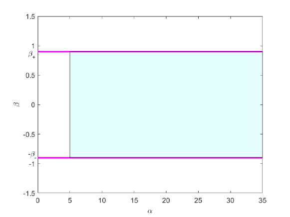
   Figure 1. Illustration of the shape of $\Omega$ (in cyan color) associated with the potentials $V_{1}(x)=i\arctan(x)$ and $V_{2}(x)=i\frac{x}{\sqrt{x^{2}+1}}$ given in (2.18).

2. $V$ is bounded at $-\infty$ and unbounded at $+\infty$: A simple choice is

   $$V(x)=i\left(e^{x}-1\right).$$

   It meets the condition (2.1) since

   $$\lim_{x\to-\infty}\mathrm{Im}\,V(x)=-1,\qquad\lim_{x\to+\infty}\mathrm{Im}\,V(x)=+\infty,$$

   and it satisfies the other conditions with $\tau_{\pm}=1$ and $\nu_{+}=0$. Depending on the behaviour of $V$ at $\pm\infty$, $\sigma_{-}^{(N)}(\alpha)$ and $\sigma_{+}^{(N)}(\alpha)$ have different decaying:

   $$\sigma_{-}^{(N)}(\alpha)\lesssim\alpha^{-\frac{N+1}{4}},\qquad\sigma_{+}^{(N)}(\alpha)=\alpha^{\frac{2-N}{4}+\varepsilon}.$$

   Here, to estimate $\sigma_{+}^{(N)}$, we just notice that $\delta_{\alpha}^{+}$ is the solution of the equation

   $$\mathrm{Im}\,V(x)=\alpha^{\frac{3+\varepsilon_{1}}{4+\varepsilon_{1}}},$$

   therefore, by writing $\frac{3+\varepsilon_{1}}{4+\varepsilon_{1}}\eqqcolon\frac{3}{4}+\varepsilon$, we get the above estimate, since

   $$\sigma_{+}^{(N)}(\alpha)=\alpha^{-\frac{N+1}{4}}\displaystyle\sup_{x\in[0,\delta_{\alpha}^{+}]}|V(x)|=\alpha^{-\frac{N+1}{4}}\mathrm{Im}\,V\left(\delta_{\alpha}^{+}\right)=\alpha^{\frac{3+\varepsilon_{1}}{4+\varepsilon_{1}}-\frac{N+1}{4}}.$$

   Then, for any $N\in\mathbb{N}_{3}$ and for any $\beta_{-}\in[0,1)$ and $\beta_{+}\in\mathbb{R}_{0}^{+}$, there exists a family $(\Psi_{\lambda,N})$ such that

   $$\frac{\|(H_{V}-\lambda)\Psi_{\lambda,N}\|}{\|\Psi_{\lambda,N}\|}\lesssim\alpha^{\frac{2-N}{4}+\varepsilon},$$

   for all $\displaystyle\lambda\in\Omega:=\left\{\alpha+i\beta\in\mathbb{C}:\alpha\gtrsim 1\text{ and }\beta\in[-\beta_{-},\beta_{+}]\subset(-1,+\infty)\right\}$.

Example 2 (Potentials with logarithmic imaginary).

Consider $V\in W^{N+3,\infty}_{\textup{loc}}(\mathbb{R})$, with $N\geq\leavevmode\nobreak\ 0$, satisfying Assumption I with $\tau_{\pm}(x)=\left(x^{2}+1\right)^{-\frac{1}{2}}$, which satisfy (2.3) with $\nu_{\pm}=-1$, that has the form

$$V(x)=\mathrm{Re}\,V(x)+i\ln\left(x+\sqrt{x^{2}+1}\right),$$

where

$$\left|\mathrm{Re}\,V(x)\right|\lesssim|x|^{\rho}\ln\left(|x|\right)^{4},\qquad|x|\gtrsim 1,\text{ with some }\rho<\frac{4}{3}.$$

The condition $\rho<\frac{4}{3}$ is sufficient to guarantee (2.5). For instance, $\mathrm{Re}\,V(x)$ is a polynomial of degree $\rho$. The range such that the constants $\beta_{\pm}$ in Theorem 2.1 can be taken is $\mathbb{R}_{0}^{+}$ since

$$\lim_{x\to-\infty}\mathrm{Im}\,V(x)=-\infty,\qquad\lim_{x\to+\infty}\mathrm{Im}\,V(x)=+\infty.$$

Concerning $\sigma_{\pm}^{(N)}(\alpha)$, since the functions $\tau_{\pm}(x)^{N+1}|V(x)|$ are bounded on $\mathbb{R}$ for any $N\geq 1$ (or for any $N\geq 0$ if $\rho<1$), we do not need to compute $\delta_{\alpha}^{\pm}$ in this situation. Accordingly, for any $N\in\mathbb{N}_{1}$ and for any $\beta_{\pm}\in\mathbb{R}_{0}^{+}$, there exists a family $(\Psi_{\lambda,N})$ such that

$$\frac{\|(H_{V}-\lambda)\Psi_{\lambda,N}\|}{\|\Psi_{\lambda,N}\|}\lesssim\alpha^{-\frac{N+1}{4}},$$

for all $\displaystyle\lambda\in\Omega:=\left\{\alpha+i\beta\in\mathbb{C}:\alpha\gtrsim 1\text{ and }\beta\in[-\beta_{-},\beta_{+}]\subset\mathbb{R}\right\}$.

Example 3 (Polynomial-like potentials).

Let us take a look at the potential $V\in W^{N+3,\infty}_{\textup{loc}}(\mathbb{R})$, with $N\geq 0$, satisfying Assumption I with $\tau_{\pm}(x)=(x^{2}+1)^{-\frac{1}{2}}$ and having the form

$$|\mathrm{Re}\,V(x)|\lesssim|x|^{\rho},\qquad|\mathrm{Im}\,V(x)|\approx|x|^{\gamma},\qquad|x|\gtrsim 1,$$

with $\rho\in\mathbb{R}$ and $\gamma\geq 0$. For examples, $\mathrm{Re}\,V$ and $\mathrm{Im}\,V$ are, respectively, the polynomials of degree $\rho$ and $\gamma$. It is necessary to assume that $\gamma\geq 0$ in order to meet the condition (2.1) and we assume further that $\gamma>\frac{3\rho-4}{4}$ such that (2.5) is satisfied. Accordingly, the fast growth of $|\mathrm{Re}\,V(x)|$ require the fast growth of $\mathrm{Im}\,V(x)$. In particular if $\rho<\frac{4}{3}$ (i.e. $|\mathrm{Re}\,V(x)|$ grows slower that $|x|^{\frac{4}{3}}$) even a bounded $\mathrm{Im}\,V$ fits. In order to apply Theorem 2.1, let us denote the quantity

$$\omega:=\max\{\rho,\gamma\}.$$

Clearly, $\omega\geq 0$ and $V$ is bounded if and only if $\omega=0$. When $|V|$ is unbounded, $\delta_{\alpha}^{\pm}$ is the solution of the equation

$$|x|^{\gamma}\left(x^{2}+1\right)^{\frac{1}{2}}=\alpha^{\frac{3+\varepsilon_{1}}{4+\varepsilon_{1}}}.$$

When $x$ is large enough, since $|x|^{\gamma}\left(x^{2}+1\right)^{\frac{1}{2}}\approx|x|^{\gamma+1}$, we can approximate the solution of the above equation with the notation $\approx$ introduced in Subsection 1.2 as follows

$$\delta^{-}_{\alpha}=\delta^{+}_{\alpha}=\delta\approx\alpha^{\frac{3}{4(\gamma+1)}+\varepsilon}.$$

Here $\varepsilon>0$ can be made arbitrary small by an appropriate choice of small $\varepsilon_{1}>0$. Hence Theorem 2.1 results that

$$\frac{\|(H_{V}-\lambda)\Psi_{\lambda,N}\|}{\|\Psi_{\lambda,N}\|}=\left\{\begin{aligned} &\mathcal{O}\left(\alpha^{-\frac{N+1}{4}}\right),\qquad&\omega\leq N+1,\\ &\mathcal{O}\left(\alpha^{-\frac{N+1}{4}+\frac{3}{4}\frac{\omega-N-1}{\gamma+1}+\varepsilon(\omega-N-1)}\right),\qquad&\omega>N+1,\end{aligned}\right.$$ (2.19)

as $\alpha\to+\infty$ and $\beta\in[-\beta_{-},\beta_{+}]$ which is mentioned in (2.7). When $V$ is bounded, the decay is also included in the case $\omega\leq N+1$. To improve the decay rate in the second case, we let $\varepsilon$ be small enough and notice that from the condition $\gamma>\frac{3\rho-4}{4}$, we can control the other term by

$$\frac{3}{4}\frac{\omega-N-1}{\gamma+1}<\left\{\begin{aligned} &\frac{3}{4}\qquad&&\text{if }\gamma\geq\rho,\\ &1\qquad&&\text{if }\gamma<\rho.\end{aligned}\right.$$

By considering $\varepsilon$ very small in (2.19), we see that the pseudomode with $N=3$ (i.e. we require at least $V\in W^{6,\infty}_{\textup{loc}}(\mathbb{R})$) is sufficient to treat all polynomial-like potentials. Comparing this with the same results for Schrödinger operators in [21, Ex. 3.8] and Dirac operators in [20, Ex. 2], more terms in the pseudomode expansion are needed in the higher order differential operators.

Example 4 (Super-exponential potential).

We devote the other application of Theorem 2.1 for the potential that is smooth and grow very fast at infinity, that is

$$V(x)=\cosh(\sinh(x))+i\sinh(\sinh(x)).$$

The Assumption I is satisfied with $\tau_{\pm}(x)=\cosh(x)$ and $\nu_{\pm}=0$. We emphasize here that [21, Asm. I] can not cover this potential, more precisely [21, Cond. 3.2] can not be satisfied. The solution $\delta$ of the equation $\frac{|\sinh(\sinh(\pm\delta))|}{\cosh(\delta)}=\alpha^{\frac{3+\varepsilon_{1}}{4+\varepsilon_{1}}}$ can be estimated as follows

$$\delta_{\alpha}^{-}=\delta_{\alpha}^{+}=\delta\approx\ln\left(\ln\left(\alpha^{\frac{3}{4}+\varepsilon}\right)\right),$$

where $\varepsilon$ can be made arbitrary small by an appropriate choice of small $\varepsilon_{1}$. Then, for arbitrary $\beta_{\pm}\in\mathbb{R}_{0}^{+}$ and for all $\beta\in[-\beta_{-},\beta_{+}]\subset\mathbb{R}$, the pseudomodes with $N\geq 3$ leads to a decay

$$\frac{\|(H_{V}-\lambda)\Psi_{\lambda,N}\|}{\|\Psi_{\lambda,N}\|}=\mathcal{O}\left(\alpha^{\frac{2-N}{4}+2\varepsilon}\right),\qquad\text{ as }\alpha\to+\infty.$$

Example 5 (Decaying potentials).

Consider a class of potentials with the asymptotic behaviour

$$V(x)=i\frac{\textup{sgn}(x)}{|x|^{\gamma}},\qquad|x|\gtrsim 1,\ 0<\gamma<1,$$ (2.20)

which spoils the assumption (2.1). However, the analysis in Subsection 4.4 shows us that we can apply the same construction as for Theorem 2.1 to set up pseudomodes for large pseudoeigenvalues $\lambda=\alpha+i\beta$ satisfying

$$|\beta|\alpha^{\frac{3}{4}\frac{\gamma}{1-\gamma}}=o(1),\qquad\text{ as }\alpha\to+\infty,\,|\beta|\to 0.$$ (2.21)

Furthermore, if we make the restriction (2.21) stronger by considering

$$|\beta|\lesssim\alpha^{-\frac{3}{4}\frac{\gamma}{1-\gamma}-\varepsilon},\qquad\text{ as }\alpha\to+\infty,$$

we will have a decay

$$\frac{\|(H_{V}-\lambda)\Psi_{\lambda,N}\|}{\|\Psi_{\lambda,N}\|}=\mathcal{O}\left(\alpha^{-\frac{N+1}{4}}\right),\qquad\text{ as }\alpha\to+\infty.$$

In other words, the $\Omega$ in the main problem (1.2) can be described by (see Figure 2)

$$\Omega=\left\{\alpha+i\beta\in\mathbb{C}:\alpha\gtrsim 1,\ |\beta|\lesssim\alpha^{-\frac{3}{4}\frac{\gamma}{1-\gamma}-\varepsilon}\right\}.$$

In [21, Eqn. 3.24], Krejčiřík and Siegl used this type of decaying potential to give a natural Laptev-Safronov eigenvalues bounds for the Schrödinger operator with $L^{p}$-potentials ($p>1$) which appears in [23, Theorem 5]. Here, in the same manner, by observing that $V\in L^{p}$ if $\gamma p>1$, it yields that

$$\frac{3}{4}\frac{\gamma}{1-\gamma}(p-1)=\frac{3}{4}\frac{\gamma p-\gamma}{1-\gamma}>\frac{3}{4}.$$

From this, we obtain a bound for $\Omega$, which is also a bound for the distribution of the eigenvalues of the biharmonic operator

$$\Omega\subset\left\{\alpha+i\beta\in\mathbb{C}:|\beta|^{p-1}=o\left(\alpha^{-\frac{3}{4}}\right),\alpha\to+\infty\right\}.$$

If the power of $\alpha$ is $-\frac{1}{2}$ in the Schrödinger case, this power is replaced by $-\frac{3}{4}$ for the biharmonic one.

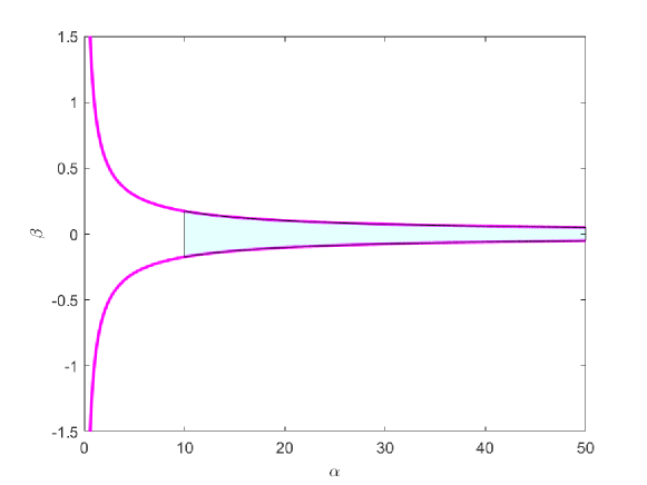
Figure 2. Illustrations of the shapes of $\Omega$ (in cyan color) associated with the potential $V(x)=i\frac{\textup{sgn}(x)}{|x|^{\gamma}}$ given in (2.20) with $\gamma=\frac{1}{2}$. The curves are the graphs of $\beta=\pm\alpha^{-\frac{3}{4}-\frac{1}{100}}$.

2.2.2. Application of Theorem 2.2

Now, we would like to apply Theorem 2.2 to study the elementary potentials considered in Subsection 2.2.1. It is worthwhile to mention here that the below Examples 6 and 8 can not be covered by [21, Cond. 5.2] or [20, Cond. 4.3].

Example 6.

Let us consider again the logarithmic potential $V\in W_{\mathrm{loc}}^{N,2}(\mathbb{R}_{0}^{+})$ that has the following behaviour

$$V(x):=i\ln(x),\qquad x\gtrsim 1.$$ (2.22)

All conditions of Assumption II are satisfied with $\tau(x)=\left(x^{2}+1\right)^{-\frac{1}{2}}\approx x^{-1}$ ($\nu=-1$ in (2.3)) as $x\gtrsim 1$, and for instance $t_{1}=0$ and some $t_{2}>0$. Given $\beta>0$, then $x_{\beta}>0$ is determined by the relation $x_{\beta}=e^{\beta}$. Since $\mathrm{Re}\,V(x)=0$, the conditions (2.16) and (2.17) are assured iff

$$\beta^{\frac{4}{5}}\exp\left(-\frac{4}{5}\beta\right)\lesssim\alpha\lesssim\beta^{\frac{4}{3}-\varepsilon}\exp\left(\left(\frac{4}{3}-\varepsilon\right)\beta\right),$$ (2.23)

where $\varepsilon>0$ can be chosen arbitrarily small by an appropriate choice of small $\varepsilon_{1}$. Then, thanks to the second inequality in (2.23), we have

$$\kappa(\beta)\lesssim\left\{\begin{aligned} &\exp\left(-c\beta^{\frac{3\varepsilon}{4}-1}\exp\left(\beta^{\frac{3\varepsilon}{4}}\right)\right)\qquad&&\text{if }\alpha>\beta,\\ &\exp\left(-c\beta^{-\frac{3}{4}}\exp\left(\beta\right)\right)\qquad&&\text{if }\alpha\leq\beta.\end{aligned}\right.$$

Let us present here the detail of estimating $\sigma^{(N)}$ for $N\geq 1$ (for $N=0$, it is analogous). If $\alpha>\beta$, we estimate straightforwardly as follows

$$\sigma^{(N)}(\beta) \lesssim\sum_{k=0}^{3N-1}\sum_{j=1}^{k+N+1}\frac{\exp\left(-(k+N+1)\beta\right)\beta^{j}}{\alpha^{\frac{k+N-3}{4}+j}}\lesssim\sum_{k=0}^{3N-1}\frac{\beta\exp\left(-(k+N+1)\beta\right)}{\beta^{\frac{k+N+1}{4}}}$$

$$\lesssim\beta^{\frac{3-N}{4}}\exp\left(-(N+1)\beta\right).$$

When $\alpha\leq\beta$, we employ the first inequality in (2.23), we obtain

$$\sigma^{(N)}(\beta) \lesssim\sum_{k=0}^{3N-1}\frac{\exp\left(-(k+N+1)\beta\right)\beta^{k+N+1}}{\alpha^{\frac{k+N-3}{4}+k+N+1}}\lesssim\sum_{k=0}^{3N-1}\frac{\beta^{k+N+1}\exp\left(-(k+N+1)\beta\right)}{\left[\beta^{\frac{4}{5}}\exp\left(-\frac{4}{5}\beta\right)\right]^{\frac{5}{4}k+\frac{5}{4}N+\frac{1}{4}}}$$

$$\lesssim\beta^{\frac{4}{5}}\exp\left(-\frac{4}{5}\beta\right).$$

In summary, Theorem 2.2 provides the pseudomodes such that

$$\frac{\|(H_{V}-\lambda)\Psi_{\lambda,N}\|}{\|\Psi_{\lambda,N}\|}=\left\{\begin{aligned} &\mathcal{O}\left(\beta^{\frac{3-N}{4}}\exp(-(N+1)\beta)\right)\qquad&&\text{ if }\alpha>\beta,\\ &\mathcal{O}\left(\beta^{\frac{4}{5}}\exp\left(-\frac{4}{5}\beta\right)\right)\qquad&&\text{ if }\alpha\leq\beta,\end{aligned}\right.$$

where $\lambda\to\infty$ in

$$\Omega:=\left\{\alpha+i\beta\in\mathbb{C}:\beta\gtrsim 1\text{ and }\beta^{\frac{4}{5}}\exp\left(-\frac{4}{5}\beta\right)\lesssim\alpha\lesssim\beta^{\frac{4}{3}-\varepsilon}\exp\left(\left(\frac{4}{3}-\varepsilon\right)\beta\right)\right\}.$$ (2.24)

From the definition of $\Omega$, we see that the pseudospectral region contains even points which stay very close to the line $\alpha=0$ (see Figure 3 3(a)).

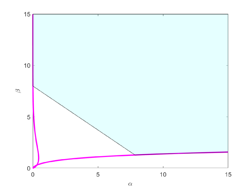
(a) $V(x)=i\ln(x)$.

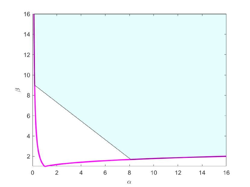
(b) $V(x)=ix^{\frac{1}{2}}$.

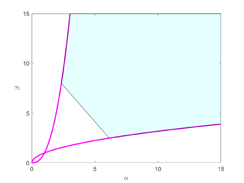
(c) $V(x)=ix^{2}$.

Figure 3. Illustration of the shapes of $\Omega$ (in cyan color) with the logarithmic function $V$ given in (2.22) and the polynomial $V$ given in (2.25): (a) $V(x)=i\ln(x)$: The curves are the graphs of $\alpha=\beta^{\frac{4}{5}}\exp\left(-\frac{4}{5}\beta\right)$ and $\alpha=\beta^{\frac{4}{3}-\frac{1}{100}}\exp\left(\left(\frac{4}{3}-\frac{1}{100}\right)\beta\right)$, (b) $V(x)=ix^{\frac{1}{2}}$: The curves are the graphs of $\alpha=\beta^{-\frac{4}{5}}$ and $\alpha=\beta^{4-\frac{1}{100}}$, (c) $V(x)=ix^{2}$: The curves are the graphs of $\alpha=\beta^{\frac{2}{5}+\frac{1}{100}}$ and $\alpha=\beta^{2-\frac{1}{100}}$.

Example 7.

Next, we want to study the polynomial potential on $\mathbb{R}_{0}^{+}$:

$$V(x)=ix^{\gamma},\qquad x\gtrsim 1$$ (2.25)

where $\gamma>0$. All the conditions of Assumption II are satisfied with $\tau$ chosen as in Example 6 and we can choose $t_{1}=t_{2}=0$. Given $\beta>0$, then $x_{\beta}>0$ is determined by $x_{\beta}=\beta^{\frac{1}{\gamma}}$. It is straightforward to check that the conditions (2.16) and (2.17) holds if we choose $\alpha=\alpha(\beta)$ in the following way

$$\beta^{\frac{4}{5}\left(1-\frac{1}{\gamma}\right)}\lesssim\alpha\lesssim\beta^{\frac{4}{3}\left(1+\frac{1}{\gamma}\right)-\varepsilon},$$ (2.26)

where $\varepsilon>0$ can be chosen arbitrarily small by an appropriate choice of small $\varepsilon_{1}$. By the second inequality in (2.26), the term $\kappa(\beta)$ can be estimated as

$$\kappa(\beta)\lesssim\left\{\begin{aligned} &\exp\left(-c\beta^{\frac{3\varepsilon}{4}}\right)\qquad&&\text{if }\alpha>\beta,\\ &\exp\left(-c\beta^{\frac{1}{\gamma}+\frac{1}{4}}\right)\qquad&&\text{if }\alpha\leq\beta.\end{aligned}\right.$$

By performing the estimate analogously in Example 6 to control $\sigma^{(N)}(\beta)$ and consider $N$ large enough, we obtain the decay in two following cases.

1. If $0<\gamma<1$, we get

   $$\frac{\|(H_{V}-\lambda)\Psi_{\lambda,N}\|}{\|\Psi_{\lambda,N}\|}=\left\{\begin{aligned} &\mathcal{O}\left(\beta^{-(N+1)\left(\frac{1}{\gamma}+\frac{1}{4}\right)+1}\right)\qquad&&\text{ if }\alpha>\beta,\\ &\mathcal{O}\left(\beta^{\frac{4}{5}\left(1-\frac{1}{\gamma}\right)}\right)\qquad&&\text{ if }\alpha\leq\beta,\end{aligned}\right.$$

   when $\lambda\to\infty$ in the region

   $$\Omega:=\left\{\alpha+i\beta\in\mathbb{C}:\beta\gtrsim 1\text{ and }\beta^{\frac{4}{5}\left(1-\frac{1}{\gamma}\right)}\lesssim\alpha\lesssim\beta^{\frac{4}{3}\left(1+\frac{1}{\gamma}\right)-\varepsilon}\right\}.$$

   The shape of this region as $\gamma=\frac{1}{2}$ is sketched in Figure 3 3(b).

2. If $\gamma>1$, we need to strengthen the first inequality in (2.26) to obtain the decay of $\sigma(\beta)$ and thus

   $$\frac{\|(H_{V}-\lambda)\Psi_{\lambda,N}\|}{\|\Psi_{\lambda,N}\|}=\left\{\begin{aligned} &\mathcal{O}\left(\beta^{-(N+1)\left(\frac{1}{\gamma}+\frac{1}{4}\right)+1}\right)\qquad&&\text{ if }\alpha>\beta,\\ &\mathcal{O}\left(\beta^{\frac{4}{5}\left(1-\frac{1}{\gamma}\right)-\varepsilon\frac{5N+1}{4}}\right)\qquad&&\text{ if }\alpha\leq\beta,\end{aligned}\right.$$

   as $\lambda\to\infty$ in

   $$\Omega:=\left\{\alpha+i\beta\in\mathbb{C}:\beta\gtrsim 1\text{ and }\beta^{\frac{4}{5}\left(1-\frac{1}{\gamma}\right)+\varepsilon}\lesssim\alpha\lesssim\beta^{\frac{4}{3}\left(1+\frac{1}{\gamma}\right)-\varepsilon}\right\}.$$

   The shape of this region as $\gamma=2$ is given in Figure 3 3(c).

Example 8.

The final example that we want to study is the superexponential potential

$$V(x)=ie^{e^{x}},\qquad x\gtrsim 1.$$ (2.27)

All conditions of Assumption II are satisfied with $\tau(x)=e^{x}$, $\nu=0$ and $t_{1}=t_{2}=0$. Given $\beta>0$, the turning point $x_{\beta}$ is determined by the relation

$$x_{\beta}=\ln\left(\ln(\beta)\right),\qquad\beta\gtrsim 1.$$

Then $\tau(x_{\beta})=\ln(\beta)$ and the conditions (2.17) are equivalent to

$$\left[\beta\ln(\beta)\right]^{\frac{4}{5}}\lesssim\alpha\lesssim\left[\frac{\beta}{\ln(\beta)}\right]^{\frac{4}{3}-\varepsilon},$$ (2.28)

where $\varepsilon>0$ can be chosen arbitrarily small by an appropriate choice of small $\varepsilon_{1}$ as above examples. By the second inequality in (2.28), we obtain the estimate for $\kappa(\beta)$:

$$\kappa(\beta)\lesssim\left\{\begin{aligned} &\exp\left(-c\left(\frac{\beta}{\ln(\beta}\right)^{\frac{3\varepsilon}{4}}\right)&&\text{if }\alpha>\beta,\\ &\exp\left(-c\frac{\beta^{\frac{1}{4}}}{\ln(\beta)}\right)&&\text{if }\alpha\leq\beta.\end{aligned}\right.$$

In order to get the decay of $\sigma^{(N)}(\beta)$, we need to strengthen the first inequality in (2.28) as follows

$$\beta^{\frac{4}{5}+\varepsilon}\ln(\beta)^{\frac{4}{5}}\lesssim\alpha\lesssim\left[\frac{\beta}{\ln(\beta)}\right]^{\frac{4}{3}-\varepsilon}.$$ (2.29)

then it yields that

$$\frac{\|(H_{V}-\lambda)\Psi_{\lambda,N}\|}{\|\Psi_{\lambda,N}\|}=\left\{\begin{aligned} &\mathcal{O}\left(\ln(\beta)^{N+1}\beta^{\frac{3-N}{4}}\right)\qquad&&\text{ if }\alpha>\beta,\\ &\mathcal{O}\left(\ln(\beta)^{\frac{4}{5}}\beta^{\frac{4}{5}-\varepsilon\frac{5N+1}{4}}\right)\qquad&&\text{ if }\alpha\leq\beta,\end{aligned}\right.$$

as $\lambda\to\infty$ in

$$\Omega:=\left\{\alpha+i\beta\in\mathbb{C}:\beta\gtrsim 1\text{ and }\beta^{\frac{4}{5}+\varepsilon}\ln(\beta)^{\frac{4}{5}}\lesssim\alpha\lesssim\left[\frac{\beta}{\ln(\beta)}\right]^{\frac{4}{3}-\varepsilon}\right\}.$$

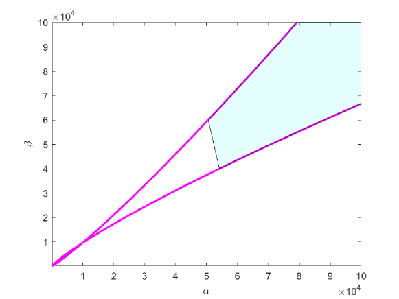
Figure 4. Illustration of the shape of $\Omega$ (in cyan color) with the superexponential $V$ given in (2.27) in which the curves are the graphs of $\alpha=\beta^{\frac{4}{5}+\frac{1}{100}}\ln(\beta)^{\frac{4}{5}}$ and $\alpha=\left[\frac{\beta}{\ln(\beta}\right]^{\frac{4}{3}-\frac{1}{100}}$.

From Figure 3 and Figure 4, we see that the pseudospectrum of the operator comes close to the imaginary axis as the potential grows slowly at infinity as logarithmic functions and root-type ones $x^{\gamma}$ with $\gamma\in(0,1)$. When the potential grows faster as polynomial and exponential functions, the pseudospectrum stay away the axes accordingly.

2.2.3. Application of Theorem 2.3

We recall some standard notions that is introduced in [22, Sec. IV]. The symbol associated with $H_{h}$ is

$$f(x,\xi)=\xi^{4}+W(x),$$

and its semi-classical pseudospectrum of $H_{h}$ is given by the closure of the set

$$\Lambda=\left\{\xi^{4}+W(x):\xi^{3}\mathrm{Im}\,W^{\prime}(x)<0\right\}.$$

Since the sign of $\xi$ can be chosen freely, we can describe $\Lambda$ as

$$\Lambda=\left\{\xi^{4}+W(x):\xi\neq 0,\ \mathrm{Im}\,W^{\prime}(x)\neq 0\right\},$$

this condition is also given in Davies’ work [7] for Schrödinger operator. Then $z\in\Lambda$ if and only if there exists $(\xi_{0},x_{0})\in\mathbb{R}^{2}$ such that $z=\xi_{0}^{4}+W(x_{0})$ with $\xi_{0}\in\mathbb{R}\setminus\{0\}$ and $\mathrm{Im}\,W^{\prime}(x_{0})\neq 0$. Taylor’s Theorem yields

$$\mathrm{Im}\,W(x)-\mathrm{Im}\,W(x_{0})=\mathrm{Im}\,W^{\prime}(x_{0})(x-x_{0})+\mathcal{O}\left(|x-x_{0}|^{2}\right).$$

Then, there exists a neighbourhood of $x_{0}$ in which the sign of the function $\mathrm{Im}\,W(x)-\leavevmode\nobreak\ \mathrm{Im}\,W(x_{0})$ changes at the point $x_{0}$ and we can apply Theorem 2.3 to obtain the pseudomode for the operator $H_{h}$ corresponding to pseudoeigenvalue $z$. Furthermore, we can extend $\Lambda$ to the set

$$\widetilde{\Lambda}=\left\{\xi^{4}+W(x)\left|\begin{aligned} &\xi\neq 0,\text{ there exists }p\in\mathbb{N}_{0}\text{ such that }\\ &\mathrm{Im}\,W^{(j)}(x)=0\text{ for all }j\neq 0,j\leq 2p\text{ and }\mathrm{Im}\,W^{(2p+1)}(x)\neq 0\end{aligned}\right.\right\}$$

which appears in the paper [26] for Schrödinger operator, and the above result remains true. In summary, we obtained the result as in the papers [7, 26] for the biharmonic operator.

3. WKB construction

3.1. The WKB expansion

Let $P_{\lambda}:\mathbb{R}\to\mathbb{C}$ be a sufficient regular function depending on the parameter $\lambda$ which will be determined later. We consider the formal conjugated operator of $\mathscr{L}_{V}-\lambda$:

$$e^{P_{\lambda}}\left(\mathscr{L}_{V}-\lambda\right)e^{-P_{\lambda}}=e^{P_{\lambda}}\left(\frac{\mathrm{d}^{4}}{\mathrm{d}x^{4}}+V(x)-\lambda\right)e^{-P_{\lambda}}=\mathcal{D}_{\lambda}+\mathcal{R}_{\lambda},$$

where $\mathcal{D}_{\lambda}$ has a differential expression and $\mathcal{R}_{\lambda}$ has a multiplication expression

$$\mathcal{D}_{\lambda}\coloneqq\frac{\mathrm{d}^{4}}{\mathrm{d}x^{4}}-4P_{\lambda}^{(1)}\frac{\mathrm{d}}{\mathrm{d}x^{3}}+6\left[\left(P_{\lambda}^{(1)}\right)^{2}-P_{\lambda}^{(2)}\right]\frac{\mathrm{d}^{2}}{\mathrm{d}x^{2}}-4\left[P_{\lambda}^{(3)}-3P_{\lambda}^{(1)}P_{\lambda}^{(2)}+\left(P_{\lambda}^{(1)}\right)^{3}\right]\frac{\mathrm{d}}{\mathrm{d}x},$$ (3.1)

$$\mathcal{R}_{\lambda}\coloneqq-P_{\lambda}^{(4)}+4P_{\lambda}^{(1)}P_{\lambda}^{(3)}+3\left(P_{\lambda}^{(2)}\right)^{2}-6\left(P_{\lambda}^{(1)}\right)^{2}P_{\lambda}^{(2)}+\left(P_{\lambda}^{(1)}\right)^{4}+V(x)-\lambda.$$

The general WKB strategy is as follows. We look for the pseudomodes in the form

$$\Psi_{\lambda}=\xi_{\lambda}e^{-P_{\lambda}},$$

where $\xi_{\lambda}$ is a cut-off function whose shape is determined later depending on the behaviour of $V$ at infinity ($\pm\infty$). From the triangular inequality, it yields that

$$\frac{\left\|\left(\mathscr{L}_{V}-\lambda\right)\Psi_{\lambda}\right\|}{\|\Psi_{\lambda}\|}=\frac{\left\|e^{-P_{\lambda}}\mathcal{D_{\lambda}}\xi_{\lambda}+\xi_{\lambda}e^{-P_{\lambda}}\mathcal{R}_{\lambda}\right\|}{\left\|\Psi_{\lambda}\right\|}\leq\frac{\left\|e^{-P_{\lambda}}\mathcal{D_{\lambda}}\xi_{\lambda}\right\|}{\left\|\Psi_{\lambda}\right\|}+\left\|\mathcal{R}_{\lambda}\right\|_{L^{\infty}(J_{\lambda})}.$$ (3.2)

Here $J_{\lambda}$ is the support of the cut-off $\xi_{\lambda}$. The WKB idea is to look for the phase $P_{\lambda}$ in the following form,

$$P_{\lambda,n}(x)=\sum_{k=-1}^{n-1}\lambda^{-k}\psi_{k}(x),\qquad n\in\mathbb{N}_{0},$$ (3.3)

where functions $\left(\psi_{k}\right)_{k\in[[-1,n-1]]}$ are to be determined by solving some ordinary differential equations (ODEs); the number $n$ is chosen later depending on the maximal possible order derivative of $V$. In principle, by letting $\lambda\to\infty$, the first term in the right hand side of (3.2) can be shown exponentially decay thanks to consideration on the support of $\xi_{\lambda}$ and the second term often decreases with the rate power of $\lambda^{-1}$. The more regular the potential is, the stronger the rate of decay in (3.2) is obtained.

Let us start with $n=0$ and put $P_{\lambda,0}$ into the formula of $\mathcal{R}_{\lambda}$ in (3.1), we obtain

$$\mathcal{R}_{\lambda,0}:=-\lambda\psi_{-1}^{(4)}+4\lambda^{2}\psi_{-1}^{(1)}\psi_{-1}^{(3)}+3\lambda^{2}\left(\psi_{-1}^{(2)}\right)^{2}-6\lambda^{3}\left(\psi_{-1}^{(1)}\right)^{2}\psi_{-1}^{(2)}+\lambda^{4}\left(\psi_{-1}^{(1)}\right)^{4}+V(x)-\lambda.$$

By solving the equation $\lambda^{4}(\psi_{-1}^{(1)})^{4}+V(x)-\lambda=0$, we often call it “eikonal” equation, the forth order of $\lambda$ in $R_{\lambda,0}$ is removed:

$$\mathcal{R}_{\lambda,0}:=-\lambda\psi_{-1}^{(4)}+4\lambda^{2}\psi_{-1}^{(1)}\psi_{-1}^{(3)}+3\lambda^{2}(\psi_{-1}^{(2)})^{2}-6\lambda^{3}(\psi_{-1}^{(1)})^{2}\psi_{-1}^{(2)}.$$ (3.4)

From this simple observation, we wish that when we increase $n$ in $P_{\lambda,n}$, the order of $\lambda$ appearing in the remainder $\mathcal{R}_{\lambda,n}$ has been reduced accordingly. For $n\in\mathbb{N}_{1}$, we replace $P_{\lambda,n}$ into $\mathcal{R}_{\lambda}$ in (3.1), we get

$$\mathcal{R}_{\lambda,n} \coloneqq-\sum_{k=-1}^{n-1}\lambda^{-k}\psi_{k}^{(4)}+4\sum_{k=-2}^{2n-2}\lambda^{-k}\sum_{\alpha_{1}+\alpha_{2}=k}\psi_{\alpha_{1}}^{(1)}\psi_{\alpha_{2}}^{(3)}+3\sum_{k=-2}^{2n-2}\lambda^{-k}\sum_{\alpha_{1}+\alpha_{2}=k}\psi_{\alpha_{1}}^{(2)}\psi_{\alpha_{2}}^{(2)}$$

$$\qquad-6\sum_{k=-3}^{3n-3}\lambda^{-k}\sum_{\alpha_{1}+\alpha_{2}+\alpha_{3}=k}\psi_{\alpha_{1}}^{(1)}\psi_{\alpha_{2}}^{(1)}\psi_{\alpha_{3}}^{(2)}+\sum_{k=-4}^{4n-4}\lambda^{-k}\sum_{\alpha_{1}+\alpha_{2}+\alpha_{3}+\alpha_{4}=k}\psi_{\alpha_{1}}^{(1)}\psi_{\alpha_{2}}^{(1)}\psi_{\alpha_{3}}^{(1)}\psi_{\alpha_{4}}^{(1)}$$

$$\qquad+V(x)-\lambda$$

$$\eqqcolon\sum_{k=-4}^{4n-4}\lambda^{-k}\phi_{k+3}.$$

Here the function $\phi_{k}$ with $k\in[[-4,4n-4]]$ are naturally defined by grouping together the terms attached with the same order of $\lambda$, with the exception of $V(x)-\lambda$ which we include in the leading order term:

$$\lambda^{4}: \left(\psi_{-1}^{(1)}\right)^{4}+\frac{V(x)-\lambda}{\lambda^{4}}\eqqcolon\phi_{-1},$$

$$\lambda^{3}: 4\left(\psi_{-1}^{(1)}\right)^{3}\psi_{0}^{(1)}-6\left(\psi_{-1}^{(1)}\right)^{2}\psi_{-1}^{(2)}\eqqcolon\phi_{0},$$

$$\lambda^{2}: 4\left(\psi_{-1}^{(1)}\right)^{3}\psi_{1}^{(1)}+6\left(\psi_{-1}^{(1)}\right)^{2}\left(\psi_{0}^{(1)}\right)^{2}-6\left(\psi_{-1}^{(1)}\right)^{2}\psi_{0}^{(2)}$$

$$\hskip 71.13188pt-12\psi_{-1}^{(1)}\psi_{0}^{(1)}\psi_{-1}^{(2)}+3\left(\psi_{-1}^{(2)}\right)^{2}+4\psi_{-1}^{(1)}\psi_{-1}^{(3)}\eqqcolon\phi_{1},$$

$$\ldots$$

For $k\in[[-3,4n-4]]$, the formulae can be written as

$$-\psi_{k}^{(4)}+4\sum_{\alpha_{1}+\alpha_{2}=k}\psi_{\alpha_{1}}^{(1)}\psi_{\alpha_{2}}^{(3)}+3\sum_{\alpha_{1}+\alpha_{2}=k}\psi_{\alpha_{1}}^{(2)}\psi_{\alpha_{2}}^{(2)}$$ (3.5)

$$-6\sum_{\alpha_{1}+\alpha_{2}+\alpha_{3}=k}\psi_{\alpha_{1}}^{(1)}\psi_{\alpha_{2}}^{(1)}\psi_{\alpha_{3}}^{(2)}+\sum_{\alpha_{1}+\alpha_{2}+\alpha_{3}+\alpha_{4}=k}\psi_{\alpha_{1}}^{(1)}\psi_{\alpha_{2}}^{(1)}\psi_{\alpha_{3}}^{(1)}\psi_{\alpha_{4}}^{(1)}\eqqcolon\phi_{k+3},$$

with the convention that $\psi_{\alpha}=0$ if $\alpha\leq-2$ or $\alpha\geq n$.

Given $n\in\mathbb{N}_{1}$, requiring $\phi_{k}=0$ for all $k\in[[-1,n-1]]$, we obtain $n+1$ ODEs which can be solved explicitly to find all $\left(\psi_{k}^{(1)}\right)_{k\in[[-1,n-1]]}$ by a recursion formula

$$\psi_{-1}^{(1)} =\pm i\lambda^{-1}\left(\lambda-V\right)^{1/4},$$ (3.6)

$$\psi_{k+1}^{(1)} =\frac{1}{4(\psi_{-1}^{(1)})^{3}}\left(\psi_{k-2}^{(4)}-4\sum_{\alpha_{1}+\alpha_{2}=k-2}\psi_{\alpha_{1}}^{(1)}\psi_{\alpha_{2}}^{(3)}-3\sum_{\alpha_{1}+\alpha_{2}=k-2}\psi_{\alpha_{1}}^{(2)}\psi_{\alpha_{2}}^{(2)}\right.$$

$$\left.\hskip 56.9055pt+6\sum_{\alpha_{1}+\alpha_{2}+\alpha_{3}=k-2}\psi_{\alpha_{1}}^{(1)}\psi_{\alpha_{2}}^{(1)}\psi_{\alpha_{3}}^{(2)}-\sum_{\begin{subarray}{c}\alpha_{1}+\alpha_{2}+\alpha_{3}+\alpha_{4}=k-2\\ \alpha_{1},\alpha_{2},\alpha_{3},\alpha_{4}\neq k+1\end{subarray}}\psi_{\alpha_{1}}^{(1)}\psi_{\alpha_{2}}^{(1)}\psi_{\alpha_{3}}^{(1)}\psi_{\alpha_{4}}^{(1)}\right),$$ (3.7)

for $k\in[[-1,n-2]]$, with the convention that $\psi_{\alpha}=0$ if $\alpha\leq-2$ or $\alpha\geq n$. After solving these ODEs, the WKB remainder is

$$\mathcal{R}_{\lambda,n}=\sum_{k=n-3}^{4n-4}\lambda^{-k}\phi_{k+3},\qquad n\in\mathbb{N}_{1}.$$ (3.8)

Since $\lambda-V(x)$ is a complex-valued function, the forth root appearing in (3.6) is considered as the principal branch of the forth root which is defined as

$$z^{\frac{1}{4}}=\frac{1}{\sqrt{2}}\left(|z|^{1/2}+\frac{1}{\sqrt{2}}\left(|z|+\mathrm{Re}\,z\right)^{1/2}\right)^{1/2}+\frac{i}{2}\frac{\mathrm{Im}\,z}{\left(|z|+\mathrm{Re}\,z\right)^{1/2}\left(|z|^{1/2}+\frac{1}{\sqrt{2}}\left(|z|+\mathrm{Re}\,z\right)^{1/2}\right)^{1/2}}.$$ (3.9)

Although there are four solutions for the eikonal equation, that is $\pm\lambda^{-1}\left(\lambda-V\right)^{1/4}$ and $\pm i\lambda^{-1}\left(\lambda-V\right)^{1/4}$, but only the latter are suitable for our pseudomodes. The choice of the sign in the definition of $\psi_{-1}^{(1)}$ will be determined by the sign of $\mathrm{Im}\,V$ at infinity (see Remark 4.6).

3.2. Structure of solutions of the transport equations and the WKB remainder

From now on, we assume that we are dealing with the plus sign in the formula of $\psi_{-1}$ in (3.6), unless otherwise stated. Let us list some first solutions of the first transport equations, $\psi_{k}^{(1)}$ for $k\geq 0$, to see which structure they are equipped with:

$$\psi_{0}^{(1)}=-\frac{3}{8}\frac{V^{(1)}}{V_{\lambda}},\qquad\psi_{1}^{(1)}=\frac{i\lambda}{V_{\lambda}^{(1/4)}}\left(\frac{5}{16}\frac{V^{(2)}}{V_{\lambda}}+\frac{45}{128}\frac{(V^{(1)})^{2}}{V_{\lambda}^{2}}\right).$$

If we continue, we will see that $\psi_{2}^{(1)}$ and $\psi_{3}^{(1)}$ has the form

$$\psi_{2}^{(1)}=\frac{\lambda^{2}}{V_{\lambda}^{\frac{2}{4}}}\left\{\frac{V^{(3)}}{V_{\lambda}},\frac{V^{(1)}V^{(2)}}{V_{\lambda}^{2}},\frac{\left(V^{(1)}\right)^{3}}{V_{\lambda}^{3}}\right\},$$

$$\psi_{3}^{(1)}=\frac{\lambda^{3}}{V_{\lambda}^{\frac{3}{4}}}\left\{\frac{V^{(4)}}{V_{\lambda}},\frac{V^{(1)}V^{(3)}}{V_{\lambda}^{2}},\frac{\left(V^{(2)}\right)^{2}}{V_{\lambda}^{2}},\frac{\left(V^{(1)}\right)^{2}V^{(2)}}{V_{\lambda}^{3}},\frac{\left(V^{(1)}\right)^{4}}{V_{\lambda}^{4}}\right\},$$

where the bracket denotes a linear combination of all elements in the bracket with complex coefficients. To estimate the transport solutions later, the coefficients attached with these elements are not important, instead the structure they share together is essential. That is: for each $k\in\mathbb{N}_{1}$, each element in the bracket of $\psi_{k}^{(1)}$ has the form

$$\frac{(V^{(1)})^{\alpha_{1}}(V^{(2)})^{\alpha_{2}}...(V^{(s)})^{\alpha_{s}}}{V_{\lambda}^{j}},$$

in which $s=k+1-j$ and all $\left(\alpha_{i}\right)_{i\in[[1,s]]}\in\mathbb{N}_{0}^{s}$ satisfy

$$\alpha_{1}+\alpha_{2}+\ldots+\alpha_{s}=j,\qquad 1\alpha_{1}+2\alpha_{2}+\ldots+s\alpha_{s}=k+1.$$

This is the content of the following lemma, but first, some notations should be introduced.

Notation 3.1.

For $j,r\in\mathbb{N}_{0}$ such that $j\leq r$, we employ the following notations

$$D_{r,j}:=\left\{\displaystyle\sum_{\alpha\in\mathcal{I}_{r,j}}c_{\alpha}(V^{(1)})^{\alpha_{1}}(V^{(2)})^{\alpha_{2}}...(V^{(r-j+1)})^{\alpha_{r-j+1}}:c_{\alpha}\in\mathbb{C}\right\},$$

where

$$\mathcal{I}_{r,j}:=\left\{\alpha\in\mathbb{N}_{0}^{r-j+1}:\sum_{p=1}^{r-j+1}p\alpha_{p}=r\text{ and }\sum_{p=1}^{r-j+1}\alpha_{p}=j\right\}\,.$$ (3.10)

When $\mathcal{I}_{r,j}=\emptyset$, we make a convention that $D_{r,j}=\{0\}$. Thus, $D_{r,0}=\{0\}$ if $r\geq 1$.

Lemma 3.2.

Let $n\in\mathbb{N}_{0}$, $V\in W_{\mathrm{loc}}^{n+3,2}(\mathbb{R})$ and functions $\left(\psi_{k}^{(1)}\right)_{k\in[[-1,n-1]]}$ be determined by (3.6) and (3.7). When $x\in\mathbb{R}$ such that $V_{\lambda}(x)\in\mathbb{C}\setminus\mathbb{R}_{0}^{-}$, then we have

$$\psi_{k}^{(m)}(x)=\frac{\lambda^{k}}{V_{\lambda}(x)^{\frac{k}{4}}}\sum_{j=0}^{k+m}\frac{d_{k+m,j}(x)}{V_{\lambda}(x)^{j}},\qquad m\in[[1,n+3-k]],\text{ with }d_{r,j}\in D_{r,j}.$$ (3.11)

Moreover, $d_{r,0}=0$ if $r\geq 1$.

The condition that the range of $V_{\lambda}$ needs to stay away from $(-\infty,0]$ is added to ensure that $V_{\lambda}^{\frac{1}{4}}$ is well-defined (i.e. non-multi-valued) and differentiable inherited from the differentiability of $V$ (since the principal branch of forth root is holomorphic on $\mathbb{C}\setminus(-\infty,0]$). From (3.4) and (3.6), the remainder when we solve up to $\psi_{-1}$ can be calculated explicitly:

$$\mathcal{R}_{\lambda,0}(x)=iV_{\lambda}(x)^{1/4}\left(\frac{1}{4}\frac{V^{(3)}(x)}{V_{\lambda}(x)}+\frac{9}{16}\frac{V^{(1)}(x)V^{(2)}(x)}{V_{\lambda}^{2}(x)}+\frac{21}{64}\frac{(V^{(1)}(x))^{3}}{V_{\lambda}^{3}(x)}\right)$$ (3.12)

$$\hskip 45.52458pt+V_{\lambda}(x)^{2/4}\left(\frac{V^{(2)}(x)}{V_{\lambda}(x)}+\frac{9}{16}\frac{(V^{(1)}(x))^{2}}{V_{\lambda}(x)^{2}}\right)+iV_{\lambda}(x)^{3/4}\left(-\frac{3}{2}\frac{V^{(1)}(x)}{V_{\lambda}(x)}\right).$$

We see that the remainder contains the elements which still share the structure mentioned above. Thanks to the recursion formula (3.7), we can show by induction that the shape of the remainder $\mathcal{R}_{\lambda,n}$ can be written by means of Notation 3.1 as follows:

Lemma 3.3.

Let $n\in\mathbb{N}_{0}$, $V\in W_{\mathrm{loc}}^{n+3,2}(\mathbb{R})$ and functions $\left(\psi_{k}^{(1)}\right)_{k\in[[-1,n-1]]}$ be determined by (3.6) and (3.7), $\left(\phi_{k}\right)_{k\in[[-1,4n-1]]}$ be as in (3.5) and $R_{\lambda,n}$ as in (3.8). When $x\in\mathbb{R}$ such that $V_{\lambda}(x)\in\mathbb{C}\setminus\mathbb{R}_{0}^{-}$, then the maximal order derivative of $V$ in $\mathcal{R}_{\lambda,n}$ is $n+3$ and

$$\mathcal{R}_{\lambda,0}(x)=\sum_{k=0}^{2}\frac{1}{V_{\lambda}(x)^{\frac{k-3}{4}}}\sum_{j=1}^{k+1}\frac{d_{k+1,j}(x)}{V_{\lambda}^{j}(x)},$$

$$\mathcal{R}_{\lambda,n}(x)=\sum_{k=0}^{3n-1}\frac{1}{V_{\lambda}(x)^{\frac{k+n-3}{4}}}\sum_{j=1}^{k+n+1}\frac{d_{k+n+1,j}(x)}{V_{\lambda}^{j}(x)},\qquad n\geq 1,\text{ with }d_{r,j}\in D_{r,j}.$$

The proofs of these lemmata is postponed to Appendix A.

4. Pseudomodes for large real pseudoeigenvalues

We reserve this section for proving Theorem 2.1. In other words, we are going to construct the pseudomode for the perturbed biharmonic operator when the real part of the spectral parameter $\lambda$ is considered largely.

From the assumptions (2.2) and (2.7), there exist constants $a_{\pm}>0$ such that, for all $\beta\in B=[-\beta_{-},\beta_{+}]$,

$$\mathrm{Im}\,V(x)-\beta\lesssim\mathrm{Im}\,V(x)\lesssim-1,\qquad x\in I^{-}\coloneqq\left\{x\in\mathbb{R}_{0}^{-}:x\leq-a_{-}\right\},$$ (4.1)

$$\mathrm{Im}\,V(x)-\beta\gtrsim\mathrm{Im}\,V(x)\gtrsim 1,\qquad x\in I^{+}\coloneqq\left\{x\in\mathbb{R}_{0}^{+}:x\geq a_{+}\right\}.$$

Notice that the constants in the above notations $\lesssim$ and $\gtrsim$ are uniformly on $\beta$. Possibly considering larger $a_{\pm}$, we assume that all the remain assumptions of Assumption I also happen on $I^{\pm}$. Furthermore, two constants $a_{\pm}$ will be used as universal constants in this section, i.e. the size of $a_{\pm}$ can be changed a finite number of times but we still keep denoting them as $a_{\pm}$.

4.1. Shapes of the cut-off functions

The cut-off function is employed to complete two tasks in our construction of pseudomodes: first, by attaching with the functions created by WKB method, the cut-off make them belong to the domain of the operator; second, the cut-off makes $(\lambda-V)^{\frac{1}{4}}$ well-defined (i.e. non-multi-valued) and differentiable in its support. In the latter, the differentiability of $(\lambda-V)^{\frac{1}{4}}$ comes from the analyticity of the forth root on $\mathbb{C}\setminus(-\infty,0]$ and the regularity of $V$ with the requirement that $\lambda-V(x)\in\mathbb{C}\setminus(-\infty,0]$ on the support of the cut-off. Let us denote by $\xi:\mathbb{R}\to[0,1]$ the cut-off function satisfying the following properties

$$\left\{\begin{aligned} &\xi\in\mathcal{C}_{0}^{\infty}(\mathbb{R}),\\ &\xi(x)=1\qquad\text{on }\left(-\delta_{\alpha}^{-}+\Delta_{\alpha}^{-},\delta_{\alpha}^{+}-\Delta_{\alpha}^{+}\right),\\ &\xi(x)=0\qquad\text{on }\mathbb{R}\setminus\left(-\delta_{\alpha}^{-},\delta_{\alpha}^{+}\right),\end{aligned}\right.$$ (4.2)

where $\delta_{\alpha}^{\pm}$ and $\Delta_{\alpha}^{\pm}<\delta_{\alpha}^{\pm}$ are $\alpha$-dependent positive numbers which will be determined later. Notice that the cut-off $\xi$ can be selected in such a way that

$$\|\xi^{(j)}\|_{L^{\infty}(\mathbb{R}_{\pm})}\lesssim\left(\Delta_{\alpha}^{\pm}\right)^{-j},\qquad j\in[[1,4]].$$ (4.3)

To simplify the notation, we introduce the following sets

$$J_{\alpha}^{-}:=\left[-\delta_{\alpha}^{-},0\right],\qquad J_{\alpha}^{+}:=\left[0,\delta_{\alpha}^{+}\right],\qquad J_{\alpha}:=J_{\alpha}^{-}\cup J_{\alpha}^{+}.$$

We use the following lemma (see the proof in [20, Lemma 3.1]) to define the boundary $\delta_{\alpha}^{\pm}$ of the cut-off $\xi$.

Lemma 4.1.

Let $g:\mathbb{R}_{0}^{+}\to\mathbb{R}_{0}^{+}$ be a continuous function and let $\alpha$ be a positive number, we define

$$\delta(\alpha):=\inf\left\{x\geq 0:g(x)=\alpha\right\}.$$

Then $\delta(\alpha)$ can be infinite $(\inf\emptyset=+\infty)$, however, when $g$ is unbounded at $+\infty$ and for all sufficiently large $\alpha>0$, the number $\delta(\alpha)$ is finite and

$$\lim_{\alpha\to+\infty}\delta(\alpha)=+\infty.$$

Furthermore, if $\alpha>g(0)$ then

$$g(x)\leq\alpha,\qquad x\in[0,\delta(\alpha)].$$

We consider the following cases:

1. When $V$ is unbounded at $\pm\infty$: From the assumption (2.5), we have

   $$\tau_{\pm}^{4+\varepsilon_{1}}(x)\lesssim\left|\mathrm{Im}\,V(x)\right|,\qquad\left|\mathrm{Re}\,V(x)\right|^{3+\varepsilon_{1}}\tau_{\pm}^{4}(x)\lesssim\left|\mathrm{Im}\,V(x)\right|^{4},\qquad x\in I^{\pm}.$$

   By choosing $\eta_{1}\in(0,1)$ such that $4+\varepsilon_{1}=\frac{4}{1-\eta_{1}}$, we will obtain, for all $x\in I^{\pm}$,

   $$\left\{\begin{aligned} &\tau_{\pm}(x)^{\frac{4}{1-\eta_{1}}}\lesssim\left|\mathrm{Im}\,V(x)\right|,\\ &\left|\mathrm{Im}\,V(x)\right|\lesssim\left|\frac{\mathrm{Im}\,V(x)}{\tau_{\pm}(x)}\right|^{\frac{4}{3+\eta_{1}}},\\ &\left|\mathrm{Re}\,V(x)\right|^{\frac{1}{1-\eta_{1}}}\lesssim\left|\frac{\mathrm{Im}\,V(x)}{\tau_{\pm}(x)}\right|^{\frac{4}{3+\eta_{1}}}.\end{aligned}\right.$$ (4.4)

2. When $V$ is bounded at $\pm\infty$, from the assumption (2.6), by choosing $\eta_{2}\in(0,1)$ such that $\frac{1}{3}-\varepsilon_{2}=\frac{1-\eta_{2}}{3+\eta_{2}}$, we have

   $$\tau_{\pm}(x)\lesssim|x|^{\frac{1-\eta_{2}}{3+\eta_{2}}},\qquad x\in I^{\pm}.$$ (4.5)

By using Lemma 4.1, we can define the boundary of the cut-off $\xi$

$$\delta_{\alpha}^{\pm}:=\inf\left\{x\geq 0:g_{\pm}(x)=\alpha\right\}$$ (4.6)

through defining functions $g_{\pm}:[0,+\infty)\to[0,+\infty)$ as follows

$$g_{\pm}(x):=\left\{\begin{aligned} &\left|\frac{\mathrm{Im}\,V(\pm x)}{\tau_{\pm}(\pm x)}\right|^{\frac{4}{3+\eta_{1}}}\qquad&&\text{ if }V\text{ is unbounded at }\pm\infty,\\ &|x|^{\frac{4}{3+\eta_{2}}}\qquad&&\text{ if }V\text{ is bounded at }\pm\infty.\end{aligned}\right.$$ (4.7)

In the latter case, since $g_{\pm}$ is strictly increasing, we can work out precisely $\delta_{\alpha}^{\pm}$ whose formula is given at Theorem 2.1. In the first case, $V$ is continuous since $V\in W^{n+3,\infty}_{\textup{loc}}(\mathbb{R})$, so are the functions $g_{\pm}$. Furthermore, thanks to $\tau_{\pm}(0)>0$, the last two conditions in (4.4), $g_{\pm}$ is unbounded at $\pm\infty$ and bounded at $0$. In practice, it is not easy to get the exact solution $\delta_{\alpha}^{\pm}$ of the equation $g_{\pm}(x)=\alpha$, instead we may approximate this solution by means of the symbol “$\approx$” introduced in the Notation 1.2 (see Examples 3 and 4).

Next, we define the remain ingredient of the cut-off $\xi$ in (4.2), that is $\Delta_{\alpha}^{\pm}$. When $V$ is unbounded at $\pm\infty$, with the aid of (2.3), there exist a constant $\kappa>0$ such that, for sufficiently large $|x|$,

$$\frac{\eta}{\tau_{\pm}(x)}\leq\frac{|x|^{-\nu_{\pm}}}{4}.$$ (4.8)

Let us define

$$\Delta_{\alpha}^{\pm}=\left\{\begin{aligned} &\frac{\eta}{\tau_{\pm}(\delta_{\alpha}^{\pm})}\qquad&&\text{if }V\text{ is unbounded at }\pm\infty,\\ &\frac{1}{4}\delta_{\alpha}^{\pm}\qquad&&\text{if }V\text{ is bounded at }\pm\infty.\end{aligned}\right.$$ (4.9)

Notice that since $\nu_{\pm}\geq-1$, from (4.8), it implies that $\Delta_{\alpha}^{\pm}\leq\delta_{\alpha}^{\pm}/4$.

Proposition 4.2.

For all sufficiently large $\alpha>0$, $\delta_{\alpha}^{\pm}$ are finite and $\displaystyle\lim_{\alpha\to+\infty}\delta_{\alpha}^{\pm}=+\infty$. Furthermore, the following hold for $\alpha\gtrsim 1$ and for all $\beta\in B$,

1. On $J_{\alpha}$,

   $$\left|\mathrm{Re}\,V(x)\right|=o(\alpha),\qquad\left|\mathrm{Im}\,V(x)\right|\lesssim\alpha,\qquad|\lambda-V(x)|\approx\alpha,$$ (4.10)

   $$\tau_{\pm}(x)\lesssim\left\{\begin{aligned} &\alpha^{\frac{1-\eta_{1}}{4}}\qquad&&\text{if }V\text{ is unbounded at }\pm\infty,\\ &\alpha^{\frac{1-\eta_{2}}{4}}\qquad&&\text{if }V\text{ is bounded at }\pm\infty.\end{aligned}\right.$$ (4.11)

2. When $V$ is unbounded at $\pm\infty$, we have

   $$\tau_{\pm}(x)\approx\tau(x),\qquad\mathrm{Im}\,V(x)\approx\mathrm{Im}\,V(\pm\delta_{\alpha}^{\pm}),\qquad x\in\mathbb{R}:|x-\delta_{\alpha}^{\pm}|\leq 2\Delta_{\alpha}^{\pm}.$$ (4.12)

Proof.

The statements related to the boundary $\delta_{\alpha}^{\pm}$ of the cut-off function $\xi$ is obtained from Lemma 4.1. We will give a proof for $x\geq 0$, the case $x\leq 0$ is analogous.

1. All the estimates in (4.10) and (4.11) will be claimed on $I^{+}\cap J_{\alpha}^{+}$. In order to have them on $J_{\alpha}^{+}$, the continuity of $V$ and $\tau_{+}$ on $[0,a_{+}]$ is employed.

   1. When $V$ is bounded at $+\infty$, the claim on the real and imaginary part of $V$ in (4.10) is obvious. The last one in (4.10) is deduced from the triangle inequality

      $$|\alpha|-|V(x)-\beta|\leq\left|\lambda-V(x)\right|\leq|\alpha|+|V(x)-\beta|,$$

      and boundedness of $B$ on $\mathbb{R}$ when $\alpha>0$ is considered largely enough. In order to estimate $\tau_{+}(x)$, we apply Lemma 4.1 with the definition of $g_{+}$ in (4.7) and the aid of (4.5), for all $x\in I^{+}\cap J_{\alpha}^{+}$,

      $$\tau_{+}(x)^{\frac{4}{1-\eta_{2}}}\lesssim|x|^{\frac{4}{3+\eta_{2}}}\leq\alpha.$$

   2. When $V$ is unbounded at $+\infty$, we apply again Lemma 4.1 with the definition of $g_{+}$ in (4.7) and the help of (4.4), we have, for all $x\in I^{+}\cap J_{\alpha}^{+}$,

      $$\left|\mathrm{Im}\,V(x)\right|\lesssim g_{+}(x)\leq\alpha,\quad\left|\mathrm{Re}\,V(x)\right|\lesssim g_{+}(x)^{1-\eta_{1}}\leq\alpha^{1-\eta_{1}}.$$

      Then the estimate for $\lambda-V$ in (4.10) is followed from

      $$\left|\alpha-\mathrm{Re}\,V(x)\right|\leq\left|\lambda-V(x)\right|\leq\left|\alpha-\mathrm{Re}\,V(x)\right|+\left|\beta-\mathrm{Im}\,V(x)\right|.$$

      The above bound of $\tau_{+}$ in (4.11) is inferred from (4.4) and Lemma 4.1 that, for all $x\in I^{+}\cap J_{\alpha}^{+}$,

      $$\tau_{+}(x)^{\frac{4}{1-\eta_{1}}}\lesssim\left|\mathrm{Im}\,V(x)\right|\lesssim g_{+}(x)\leq\alpha.$$

2. First of all, let us show that, for sufficient large $x>0$ and every $|h|\leq\frac{x^{-\nu_{+}}}{2}$, we have

   $$\tau(x+h)\approx\tau(x).$$

   Indeed, from the assumption (2.3),

   $$\left|\ln\frac{|\tau(x+h)|}{|\tau(x)|}\right|=\left|\int_{x}^{x+h}\frac{\tau^{(1)}(t)}{\tau(t)}\,\mathrm{d}t\right| \lesssim\left\{\begin{aligned} &\int_{x}^{x+h}|t|^{\nu}\,\mathrm{d}t\qquad&&h\geq 0,\\ &\int_{x+h}^{x}|t|^{\nu}\,\mathrm{d}t\qquad&&h\leq 0,\end{aligned}\right.$$

   $$\leq\left\{\begin{aligned} &h(x+h)^{\nu}\qquad&&h\geq 0,\,\nu\geq 0,\\ &hx^{\nu}\qquad&&h\geq 0,\,\nu<0,\\ &(-h)x^{\nu}\qquad&&h\leq 0,\,\nu\geq 0,\\ &(-h)(x+h)^{\nu}\qquad&&h\leq 0,\,\nu<0,\\ \end{aligned}\right.$$

   $$\lesssim 1.$$

   In the last inequality, since $\nu_{+}\geq-1$, we used the observation that, for all $|h|\leq\frac{x^{-\nu_{+}}}{2}$ and for $x>0$,

   $$\frac{x}{2}\leq x+h\leq\frac{3x}{2}.$$

   Then, the first estimate for $\tau_{+}(x)$ is deduced by replacing the above $x$ by $\delta_{\alpha}^{+}$ with the notice that $\displaystyle 2\Delta_{\alpha}^{+}\leq\frac{\left(\delta_{\alpha}^{+}\right)^{-\nu_{+}}}{2}$, thanks to (4.8) and the definition of $\Delta_{\alpha}^{+}$. We employ this idea for the function $\mathrm{Im}\,V$ as following: for large $\delta_{\alpha}^{+}$ and for all $|h|\leq 2\Delta_{\alpha}^{+}$, we have

   $$\left|\ln\frac{|\mathrm{Im}\,V(\delta_{\alpha}^{+}+h)|}{|\mathrm{Im}\,V(\delta_{\alpha}^{+})|}\right|=\left|\int_{\delta_{\alpha}^{+}}^{\delta_{\alpha}^{+}+h}\frac{\mathrm{Im}\,V^{(1)}(t)}{\mathrm{Im}\,V(t)}\,\mathrm{d}t\right| \leq\left\{\begin{aligned} &\int_{\delta_{\alpha}^{+}}^{\delta_{\alpha}^{+}+h}\tau_{+}(t)\,\mathrm{d}t&&\text{if }h\geq 0,\\ &\int_{\delta_{\alpha}^{+}+h}^{\delta_{\alpha}^{+}}\tau_{+}(t)\,\mathrm{d}t&&\text{if }h\leq 0.\end{aligned}\right.$$

   $$\lesssim\tau_{+}(\delta_{\alpha}^{+})\Delta_{\alpha}^{+}=\eta.$$

   Here, in the second inequality, we have used the estimate for $\tau_{+}$ in (4.12). Thus, the estimate for $\mathrm{Im}\,V$ in (4.12) is followed.

∎

4.2. Pseudomode estimate

Let Assumption I hold for some $N\in\mathbb{N}_{0}$. Let $\psi_{-1}^{(1)}$ be determined by (3.6) with the plus sign and $\left(\psi_{k}^{(1)}\right)_{k\in[[0,N-1]]}$ be determined by (3.7), in order to obtain the primitive functions $\left(\psi_{k}\right)_{k\in[[-1,N-1]]}$, we fix the initial data for them

$$\psi_{k}(0):=0,\qquad\forall k\in[[-1,N-1]].$$

Let us define the pseudomode for Theorem 2.1 as follows

$$\Psi_{\lambda,N}:=\xi_{\lambda}\exp(-P_{\lambda,N}),$$

where

• $\xi_{\lambda}$ is the cut-off defined in (4.2) with $\delta_{\alpha}^{\pm}$ and $\Delta_{\alpha}^{\pm}$ as in (4.6) and (4.9),

• $\displaystyle P_{\lambda,N}=\sum_{k=-1}^{N-1}\lambda^{-k}\psi_{k}(t)$ defined as in (3.3).

With the intention of estimating the pseudomode $\Psi_{\lambda,N}$ later, we firstly provide some estimates for the functions $\left(\psi_{k}^{(1)}\right)_{k\in[[-1,N-1]]}$ in the following lemma.

Lemma 4.3.

For $\alpha\gtrsim 1$ and for all $\beta\in B$, we have

$$\mathrm{Re}\,\left(\lambda\psi_{-1}^{(1)}(x)\right)\approx\frac{\mathrm{Im}\,V(x)-\beta}{\alpha^{\frac{3}{4}}}\qquad \text{on }I^{\pm}\cap J_{\alpha}^{\pm},$$ (4.13)

$$\left|\mathrm{Re}\,\left(\lambda\psi_{-1}^{(1)}(x)\right)\right|\lesssim\frac{1}{\alpha^{\frac{3}{4}}}\qquad \text{on }[-a_{-},a_{+}],$$

and for all $k\in[[-1,N-1]]$, for all $m\in[[1,3]]$ such that $k+m\geq 1$, we have

$$\left|\lambda^{-k}\psi_{k}^{(m)}(x)\right|\lesssim\frac{|V(x)|\tau_{\pm}(x)^{k+m}}{\alpha^{\frac{k}{4}+1}}\qquad \text{ on }I^{\pm}\cap J_{\alpha}^{\pm},$$ (4.14)

$$\left|\lambda^{-k}\psi_{k}^{(m)}(x)\right|\lesssim\frac{1}{\alpha^{\frac{k}{4}+1}}\qquad \text{ on }[-a_{-},a_{+}].$$

Proof.

From the formula of the eikonal solution (3.6) and the principal forth root given by (3.9), we have

$$\mathrm{Re}\,\left(\lambda\psi_{-1}^{(1)}\right)=\frac{1}{2}\frac{\mathrm{Im}\,V-\beta}{\left(|V_{\lambda}|+\alpha-\mathrm{Re}\,V\right)^{1/2}\left(|V_{\lambda}|^{1/2}+\frac{1}{\sqrt{2}}\left(|V_{\lambda}|+\alpha-\mathrm{Re}\,V\right)^{1/2}\right)^{1/2}}.$$ (4.15)

Thanks to the application of (4.10) for the denominator of $\mathrm{Re}\,\left(\lambda\psi_{-1}^{(1)}\right)$, the first estimate in (4.13) is obtained directly by the fixed sign of $\mathrm{Im}\,V-\beta$ on each $I^{-}$ and $I^{+}$ (see (4.1)), while the second one in (4.13) is attained from the continuity of $\mathrm{Im}\,V$ on $[-a_{-},a_{+}]$ and the boundedness of $B$.

For each $k\in[[-1,N-1]]$ and for each $m\in[[1,3]]$ such that $k+m\geq 1$, Lemma 3.2 and the assumption (2.2) combining with the characteristic (3.10) of the set $I_{r,j}$ yield that, on $I^{+}\cap J_{\alpha}^{+}$,

$$\left|\lambda^{-k}\psi_{k}^{(m)}\right| \leq\frac{1}{\left|V_{\lambda}\right|^{\frac{k}{4}}}\sum_{j=1}^{k+m}\frac{|d_{k+m,j}|}{|V_{\lambda}|^{j}}$$

$$\lesssim\frac{1}{|V_{\lambda}|^{\frac{k}{4}}}\sum_{j=1}^{k+m}\frac{\displaystyle\sum_{\alpha\in I_{k+m,j}}|V^{(1)}|^{\alpha_{1}}|V^{(2)}|^{\alpha_{2}}\ldots|V^{(k+m+1-j)}|^{\alpha_{k+m+1-j}}}{|V_{\lambda}|^{j}}$$

$$\lesssim\frac{\tau_{+}^{k+m}}{|V_{\lambda}|^{\frac{k}{4}}}\sum_{j=1}^{k+m}\frac{|V|^{j}}{|V_{\lambda}|^{j}}.$$

From (4.10), it implies that $|V|\lesssim\alpha\lesssim|V_{\lambda}|$ on $J_{\alpha}$. Then the first estimate in (4.14) for $x>0$ is obtained:

$$\left|\lambda^{-k}\psi_{k}^{(m)}\right|\lesssim\frac{\tau_{+}^{k+m}|V|}{|V_{\lambda}|^{\frac{k}{4}+1}}\sum_{j=0}^{k+m-1}\frac{|V|^{j}}{|V_{\lambda}|^{j}}\lesssim\frac{\tau_{+}^{k+m}|V|}{\alpha^{\frac{k}{4}+1}}.$$

On $I^{-}\cap J_{\alpha}^{-}$, all the above estimates are analogous. For $k\in[[-1,N-1]]$ and $m\in[[1,3]]$, we observe that the maximal derivatives of $V$ appearing in the expression of $\lambda^{-k}\psi_{k}^{(m)}$ is $k+m+1-1=k+m$ that is at most $N+2$. Since $V\in W_{\textup{loc}}^{N+3,\infty}(\mathbb{R})$, all the derivatives of $V$ in $\lambda^{-k}\psi_{k}^{(m)}$ are continuous. The second one in (4.14) follows immediately from the boundedness of the derivatives of $V$ on $[-a_{-},a_{+}]$. ∎

Remark 4.4 (The assumption on $\mathrm{Re}\,V$).

Let us explain why we set up the condition (2.5) on $\mathrm{Re}\,V$. We consider the polynomial potential

$$V(x)=-x^{\rho}+i\ \textup{sign}(x)|x|^{\gamma}\qquad\text{ with }\rho>0,\,\gamma>0.$$

It is obvious that the assumption (2.1) is fulfilled. In this case, we can choose $\tau_{\pm}(x)=(x^{2}+1)^{-\frac{1}{2}}$ to satisfy assumptions (2.2) and (2.4) and we have $\tau_{\pm}(x)\approx|x|^{-1}$ for $|x|\gtrsim 1$ then the condition (2.3) is satisfied with $\nu_{\pm}=-1$. The assumption (2.5) reads: there exists $\varepsilon_{1}>0$ such that

$$3\rho-4+\rho\varepsilon_{1}\leq 4\gamma.$$

We assume on the contrary that

$$3\rho-4>4\gamma.$$

By change of variable $t=\alpha^{\frac{1}{\rho}}s$, it yields that, for all $x>0$,

$$\int_{0}^{x}\left|\mathrm{Re}\,\left(\lambda\psi_{-1}^{(1)}(t)\right)\right|\,\mathrm{d}t\lesssim\int_{0}^{x}\frac{|t^{\gamma}|+|\beta|}{\left(\alpha+t^{\rho}\right)^{\frac{3}{4}}}\,\mathrm{d}t\lesssim\alpha^{\frac{4\gamma-3\rho+4}{4\rho}}\int_{0}^{+\infty}\frac{s^{\gamma}+\frac{|\beta|}{\alpha^{\gamma}}}{\left(1+s^{\rho}\right)^{\frac{3}{4}}}\,\mathrm{d}t=o(1),\qquad\alpha\to+\infty.$$

It means that the dominant part $\int_{0}^{x}\lambda\mathrm{Re}\,\left(\lambda\psi_{-1}^{(1)}(t)\right)\,\mathrm{d}t$ in the expansion of $P_{\lambda,N}$ (as we see later in the next proposition) is bounded (uniformly in $\lambda$) on $R_{+}$ and this will spoil completely the decay of our pseudomode.

Proposition 4.5.

There exists $c>0$ such that, for $\alpha\gtrsim 1$ and for all $\beta\in B$,

$$\frac{\|(\mathcal{D}_{\lambda,N}\xi)\exp(-P_{\lambda,N})\|}{\|\xi\exp(-P_{\lambda,N})\|}\lesssim\exp\left(-c\alpha^{\frac{\eta}{4}}\right),$$ (4.16)

where

• $\mathcal{D}_{\lambda,N}$ is the differential representation $D_{\lambda}$ after replacing $P$ as $P_{\lambda,N}$ in (3.1),

• $\eta:=\left\{\begin{aligned} &\eta_{1}\qquad&&\text{if }V\text{ is unbounded at }\pm\infty,\\ &\eta_{2}\qquad&&\text{if }V\text{ is bounded at }\pm\infty.\end{aligned}\right.$

Proof.

The idea of the proof is as follows.

1. We will deal with the denominator of (4.16) first by showing that it is bounded below by a constant which is independent of $\alpha$.

2. In order to handle the numerator of (4.16), we will show that the eikonal term $\lambda\psi_{-1}^{(1)}$ dominates over the other terms $\lambda^{-k}\psi_{k}^{(1)}$ with $k\geq 0$ and thus there exists constants $C_{\pm}>0$ such that, for all $x\in I^{\pm}\cap J_{\alpha}^{\pm}$,

   $$\left|\exp(-P_{\lambda,N}(x))\right|\lesssim\exp\left(-\frac{C_{\pm}}{\alpha^{3/4}}\int_{\pm a_{\pm}}^{x}\mathrm{Im}\,V(t)\,\mathrm{d}t\right).$$ (4.17)

3. From (4.17), we show that there exists a constant $c_{1}>0$ such that, for all $x\in\left[-\delta_{\alpha}^{-},-\delta_{\alpha}^{-}+\Delta_{\alpha}^{-}\right]$ and for all $x\in\left[\delta_{\alpha}^{+}-\Delta_{\alpha}^{+},\delta_{\alpha}^{+}\right]$,

   $$\left|\exp\left(-P_{\lambda,N}(x)\right)\right|\lesssim\exp\left(-c_{1}\alpha^{\frac{\eta}{4}}\right).$$ (4.18)

4. Finally, we use (4.18) to control $D_{\lambda,N}\xi$ in (4.16).

The details are as follows.

1. Let us recall that

   $$P_{\lambda,N}(x)=\sum_{k=-1}^{N-1}\int_{0}^{x}\lambda^{-k}\psi_{k}^{(1)}(t)\,\mathrm{d}t.$$

   Thanks to the estimates (4.13) and (4.14), we have the bound of (4.16),

   $$\left|\mathrm{Re}\,P_{\lambda,N}(x)\right|\lesssim\frac{1}{\alpha^{\frac{3}{4}}},\qquad x\in[0,a_{+}].$$ (4.19)

   Then, there is a constant $C_{1}>0$ such that

   $$\int_{\mathbb{R}}|\xi\exp(-P_{\lambda,n}(x))|^{2}\,\mathrm{d}x\geq\int_{0}^{a^{+}}\exp\left(-2\mathrm{Re}\,P_{\lambda,N}(x)\right)\,\mathrm{d}x\geq a_{+}\exp\left(-\frac{C_{1}}{\alpha^{3/4}}\right).$$

   Therefore, by considering large $\alpha>0$, we get

   $$\left\|\xi\exp\left(-P_{\lambda,N}\right)\right\|\gtrsim 1.$$

2. Next, we will prove (4.17). On $I^{+}\cap J^{+}_{\alpha}$, thanks to (4.14) and (4.11), we have

   $$\left|\sum_{k=0}^{N-1}\mathrm{Re}\,\left(\lambda^{-k}\psi_{k}^{(1)}(t)\right)\right| \lesssim\sum_{k=0}^{N-1}\frac{|V(t)|\tau_{+}(t)^{k+1}}{\alpha^{\frac{k}{4}+1}}=\frac{|V(t)|\tau_{+}(t)}{\alpha}\sum_{k=0}^{N-1}\left(\frac{\tau_{+}(t)}{\alpha^{\frac{1}{4}}}\right)^{k}$$

   $$\lesssim\frac{|V(t)|\tau_{+}(t)}{\alpha}.$$

   Combining this with (4.13) and (4.1), it implies that

   $$\frac{\displaystyle\left|\sum_{k=0}^{N-1}\mathrm{Re}\,\left(\lambda^{-k}\psi_{k}^{(1)}(t)\right)\right|}{\mathrm{Re}\,\left(\lambda\psi_{-1}^{(1)}(t)\right)}\lesssim\frac{|V(t)|\tau_{+}(t)}{\mathrm{Im}\,V(t)\alpha^{\frac{1}{4}}}\lesssim\left\{\begin{aligned} &\alpha^{-\frac{\eta_{1}}{4}}\qquad\text{if }V\text{ is unbounded at }+\infty,\\ &\alpha^{-\frac{\eta_{2}}{4}}\qquad\text{if }V\text{ is bounded at }+\infty.\end{aligned}\right.$$

   Indeed, we consider that cases:

   1. If $V$ is bounded at $+\infty$, the above estimate comes from (4.1) and (4.11).

   2. If $V$ is unbounded at $+\infty$, the triangular inequality leads to

      $$\frac{|V(t)|\tau_{+}(t)}{\mathrm{Im}\,V(t)\alpha^{\frac{1}{4}}}\leq\frac{|\mathrm{Re}\,V(t)|\tau_{+}(t)}{\mathrm{Im}\,V(t)\alpha^{\frac{1}{4}}}+\frac{\tau_{+}(t)}{\alpha^{\frac{1}{4}}},$$

      then (4.4), the definition of $g_{+}$ in (4.7) and Lemma 4.1 allow us to control the term with $\mathrm{Re}\,V$ as follows

      $$\frac{|\mathrm{Re}\,V(t)|\tau_{+}(t)}{\mathrm{Im}\,V(t)\alpha^{\frac{1}{4}}}\lesssim\frac{g_{+}(t)^{1-\eta_{1}}\tau_{+}(t)}{\mathrm{Im}\,V(t)\alpha^{\frac{1}{4}}}=\frac{g_{+}(t)^{\frac{1-5\eta_{1}}{4}}}{\alpha^{\frac{1}{4}}}\leq\alpha^{-\frac{5\eta_{1}}{4}}.$$

      In the last inequality, we assumed that $\varepsilon_{1}$ small enough in Assumption (2.5). Hence using (4.11) to control the term $\frac{\tau_{+}(t)}{\alpha^{\frac{1}{4}}}$, we have a conclusion.

   Therefore, (4.17) is obtained by employing (4.19) , (4.13) and (4.1). In detail, for all $x\in I^{+}\cap J_{\alpha}^{+}$, we have (with some constant $C_{+}$)

   $$\left|\exp\left(-P_{\lambda,N}(x)\right)\right| =\exp\left(-\mathrm{Re}\,P_{\lambda,N}(a_{+})-\int_{a_{+}}^{x}\sum_{k=-1}^{N-1}\mathrm{Re}\,\left(\lambda^{-k}\psi_{k}^{(1)}(t)\right)\,\mathrm{d}t\right)$$

   $$\lesssim\exp\left(-\int_{a_{+}}^{x}(1-o(1))\mathrm{Re}\,\left(\lambda\psi_{-1}^{(1)}\right)\,\mathrm{d}t\right)$$

   $$\lesssim\exp\left(-\frac{C_{+}}{\alpha^{3/4}}\int_{a_{+}}^{x}\mathrm{Im}\,V(t)\,\mathrm{d}t\right).$$

   The proof for $x\in I^{-}\cap J_{\alpha}^{-}$ is the same.

3. In order to prove (4.18), we consider two cases:

   1. If $V$ is unbounded at $+\infty$, from the property (4.12) and the definitions of $\delta_{\alpha}^{+}$ in (4.6) and $g_{+}(\delta_{\alpha}^{+})$ in (4.7), we have that, for $x\in\left[\delta_{\alpha}^{+}-\Delta_{\alpha}^{+},\delta_{\alpha}^{+}\right]$,

      $$\int_{a_{+}}^{x}\mathrm{Im}\,V(t)\,\mathrm{d}t \geq\int_{\delta_{\alpha}^{+}-2\Delta_{\alpha}^{+}}^{x}\mathrm{Im}\,V(t)\,\mathrm{d}t\gtrsim\left(\Delta_{\alpha}^{+}\right)\mathrm{Im}\,V(\delta_{\alpha}^{+})$$

      $$\gtrsim\frac{\mathrm{Im}\,V(\delta_{\alpha}^{+})}{\tau(\delta_{\alpha}^{+})}=\alpha^{\frac{3+\eta_{1}}{4}}.$$

   2. If $V$ is bounded at $+\infty$, we use the assumption (4.1) to obtain,

      $$\int_{a_{+}}^{x}\mathrm{Im}\,V(t)\,\mathrm{d}t\gtrsim\int_{\delta_{\alpha}^{+}-2\Delta_{\alpha}^{+}}^{x}\mathrm{Im}\,V(t)\,\mathrm{d}t\gtrsim\Delta_{\alpha}^{+}=\alpha^{\frac{3+\eta_{2}}{4}}.$$

   Then, (4.18) is followed directly from (4.17).

4. In order to control the terms attached with $\xi^{(\ell)}$ for $\ell\in[[1,4]]$, we notice that, for $m\in[[1,3]]$

   $$\left|P_{\lambda,N}^{(m)}(x)\right|\leq\sum_{k=-1}^{N-1}\left|\lambda^{-k}\psi_{k}^{(m)}(x)\right|\lesssim\sum_{k=-1}^{N-1}\frac{\tau_{\pm}(x)^{k+m}}{\alpha^{\frac{k}{4}}},\qquad x\in I^{\pm}\cap J_{\alpha}^{\pm}.$$

   Here we employed (4.14) and (3.6). Thanks to the upper bound of $\tau_{\pm}$ by some power of $\alpha$ in (4.11), we can bound $P_{\lambda,n}^{(m)}$ by a polynomial of $\alpha$ and thus they are also rapidly decaying when they are attached with $\exp(-c_{1}\alpha^{\frac{\eta}{4}})$. For example, we give a detail on how to deal with the terms attached with $\xi^{(4)}$ and $\xi^{(3)}$, the other terms are estimated similarly:

   1. The attached with $\xi^{(4)}$, by employing (4.3) and (4.18), we have

      $$\int_{-\delta_{\alpha}^{-}}^{-\delta_{\alpha}^{-}+\Delta_{\alpha}^{-}}|\xi^{(4)}(x)|^{2}\left|\exp\left(-P_{\lambda,N}(x)\right)\right|^{2}\,\mathrm{d}x+\int_{\delta_{\alpha}^{+}-\Delta_{\alpha}^{+}}^{\delta_{\alpha}^{+}}|\xi^{(4)}(x)|^{2}\left|\exp\left(-P_{\lambda,N}(x)\right)\right|^{2}\,\mathrm{d}x$$

      $$\lesssim\left(\Delta_{\alpha}^{-}\right)^{-7}\exp\left(-2c_{1}\alpha^{\frac{\eta}{4}}\right)+\left(\Delta_{\alpha}^{+}\right)^{-7}\exp\left(-2c_{1}\alpha^{\frac{\eta}{4}}\right).$$

      By using (4.11) for $\Delta_{\alpha}^{\pm}$ defined in (4.9) when $V$ is unbounded at $\pm\infty$ and $\delta_{\alpha}^{\pm}=\frac{\alpha^{\frac{3+\eta_{2}}{4}}}{2}$ when $V$ is bounded at $\pm\infty$, it implies that

      $$\left(\Delta_{\alpha}^{\pm}\right)^{-1}\lesssim\left\{\begin{aligned} &\alpha^{\frac{1-\eta_{1}}{4}}&&\text{if }V\text{ is unbounded at }\pm\infty,\\ &\alpha^{-\frac{3+\eta_{2}}{4}}&&\text{if }V\text{ is bounded at }\pm\infty.\end{aligned}\right.$$

      Therefore, there exists $c_{2}>0$ such that

      $$\left\|\xi^{(4)}\exp\left(-P_{\lambda,N}(x)\right)\right\|\lesssim\exp\left(-c_{2}\alpha^{\frac{\eta}{4}}\right).$$

   2. The attached with $\xi^{(3)}$, we have

      $$\left|\xi^{(3)}(x)P_{\lambda,N}^{(1)}\exp\left(-P_{\lambda,N}(x)\right)\right| \lesssim\left(\Delta_{\alpha}^{\pm}\right)^{-3}\left(\sum_{k=-1}^{N-1}\frac{\tau_{+}(x)^{k+1}}{\alpha^{\frac{k}{4}}}\right)\exp\left(-c_{1}\alpha^{\frac{\eta}{4}}\right)$$

      $$\lesssim\left(\Delta_{\alpha}^{\pm}\right)^{-3}\left(\sum_{k=-1}^{N-1}\alpha^{\frac{(k+1)(1-\eta)-k}{4}}\right)\exp(-c_{1}\alpha^{\frac{\eta}{4}})$$

      $$\lesssim\exp\left(-c_{3}\alpha^{\frac{\eta}{4}}\right).$$

   Consequently, we put everything together, we obtain (4.16).

∎

4.3. Remainder estimate (Proof of Theorem 2.1)

Obviously, $\Psi_{\lambda,N}$ belongs to the domain of $\mathscr{L}_{V}$ because of its support. By the estimate (3.2) and Proposition 4.5, we have

$$\frac{\|(\mathscr{L}_{V}-\lambda)\Psi_{\lambda,N}\|}{\|\Psi_{\lambda,N}\|}\lesssim\exp(-c\alpha^{\frac{\eta}{4}})+\|\mathcal{R}_{\lambda,N}\|_{L^{\infty}(J_{\alpha})}.$$

Let $n=N$ in Lemma 3.3, estimate as in the proof of Lemma 4.3 and employ (4.11), it yields that, for $N\geq 1$,

$$\left|\mathcal{R}_{\lambda,N}(x)\right| \lesssim\sum_{k=0}^{3N-1}\frac{1}{|V_{\lambda}|^{\frac{k+N-3}{4}}}\sum_{j=1}^{k+N+1}\frac{|d_{k+N+1,j}|}{|V_{\lambda}|^{j}}\lesssim\sum_{k=0}^{3N-1}\frac{\tau_{\pm}(x)^{k+N+1}}{|V_{\lambda}|^{\frac{k+N-3}{4}}}\sum_{j=1}^{k+N+1}\frac{|V(x)|^{j}}{|V_{\lambda}|^{j}}$$

$$\lesssim\sum_{k=0}^{3N-1}\frac{\tau_{\pm}(x)^{k+N+1}|V(x)|}{|V_{\lambda}|^{\frac{k+N+1}{4}}}\lesssim\frac{|V(x)|\tau_{\pm}(x)^{N+1}}{\alpha^{\frac{N+1}{4}}},\qquad x\in I^{\pm}\cap J_{\lambda}^{\pm}.$$

Similarly, since $V\in W^{N+3,\infty}_{\textup{loc}}(\mathbb{R})$, we have the following estimate on the compact set $[-a_{-},a_{+}]$:

$$\left|\mathcal{R}_{\lambda,N}(x)\right|\lesssim\alpha^{-\frac{N+1}{4}},\qquad x\in[-a_{-},a_{+}].$$

Likewise, with the same reason, we have the same estimate for $N=0$. Thus, the estimate (2.8) is followed for all $N\geq 0$.

Remark 4.6.

From the above construction, we see that if we change the sign of $\mathrm{Im}\,V$ in condition (2.1) as follows

$$\limsup_{x\to+\infty}\mathrm{Im}\,V(x)<0<\liminf_{x\to-\infty}\mathrm{Im}\,V(x);$$ (4.20)

then the previous analysis still works. Indeed, what we need to do is just to choose the minus sign in the formula of $\psi_{-1}^{(1)}$ in (3.6). Then, we have

$$\mathrm{Re}\,\left(\lambda\psi_{-1}^{(1)}\right)=\frac{1}{2}\frac{\beta-\mathrm{Im}\,V}{\left(|V_{\lambda}|+\alpha-\mathrm{Re}\,V\right)^{1/2}\left(|V_{\lambda}|^{1/2}+\frac{1}{\sqrt{2}}\left(|V_{\lambda}|+\alpha-\mathrm{Re}\,V\right)^{1/2}\right)^{1/2}}.$$

By fixing $\beta_{\pm}\in\mathbb{R}_{0}^{+}$ such that

$$\limsup_{x\to+\infty}\mathrm{Im}\,V(x)<-\beta_{-}\text{ and }\beta_{+}<\liminf_{x\to-\infty}\mathrm{Im}\,V(x),$$

then there exist constants $a_{\pm}>0$ such that, for all $\beta\in B=[-\beta_{-},\beta_{+}]$,

$$\mathrm{Im}\,V(x)-\beta\lesssim\mathrm{Im}\,V(x)\lesssim-1,\qquad x\in I^{+}\coloneqq\left\{x\in\mathbb{R}_{0}^{+}:x\geq a_{+}\right\},$$

$$\mathrm{Im}\,V(x)-\beta\gtrsim\mathrm{Im}\,V(x)\gtrsim 1,\qquad x\in I^{-}\coloneqq\left\{x\in\mathbb{R}_{0}^{-}:x\leq-a_{-}\right\}.$$

By repeating the procedure when proving (4.13), we have

$$\mathrm{Re}\,\left(\lambda\psi_{-1}^{(1)}(x)\right)\approx\frac{\beta-\mathrm{Im}\,V(x)}{\alpha^{\frac{3}{4}}}\gtrsim-\frac{\mathrm{Im}\,V(x)}{\alpha^{\frac{3}{4}}}\qquad \text{ on }I^{+}\cap J_{\alpha}^{+},$$ (4.21)

$$\mathrm{Re}\,\left(\lambda\psi_{-1}^{(1)}(x)\right)\approx\frac{\beta-\mathrm{Im}\,V(x)}{\alpha^{\frac{3}{4}}}\lesssim-\frac{\mathrm{Im}\,V(x)}{\alpha^{\frac{3}{4}}}\qquad \text{ on }I^{-}\cap J_{\alpha}^{-}.$$

Therefore, the pseudomode now possesses the right sign for the decay. Although all the other terms $\left(\psi_{k}^{(1)}\right)_{0\leq k\leq N-1}$ also change their signs accordingly, but it does not matter because they are all estimated with the absolute value.

4.4. Decaying potentials

We reserve this section for constructing the pseudomodes for the potentials in Example 5. Since the condition 2.1 is not met by the decaying of the potentials, we can not apply directly the previous constructions. However, the shape of the pseudomodes is the same as in the beginning of Subsection 4.2, just the definition of $\delta_{\lambda}^{\pm}$ (replace for $\delta_{\alpha}^{\pm}$) should be defined differently. In the coming paragraphs, when we say $\lambda=\alpha+i\beta\to\infty$, we mean $\alpha\to+\infty$ and $|\beta|\to 0$ ($\beta$ can be zero). Let $a_{+}>0$ such that

$$\mathrm{Im}\,V(x)=|x|^{-\gamma},\qquad x\geq a_{+}.$$

We seek for the boundary $\delta_{\lambda}^{+}$ of the cut-off such that the first term in the expansion very large when $\lambda\to\infty$. Since $V$ is bounded, we still have $|\lambda-V(x)|\approx\alpha$, thus, for $x>a_{+}$,

$$\int_{a_{+}}^{x}\mathrm{Re}\,\left(\lambda\psi_{-1}^{(1)}(t)\right)\,\mathrm{d}t\gtrsim\frac{1}{\alpha^{\frac{3}{4}}}\int_{a_{+}}^{x}\left[\mathrm{Im}\,V(t)-\beta\right]\,\mathrm{d}t=\frac{x^{1-\gamma}\left[\frac{1}{1-\gamma}-\beta x^{\gamma}\right]-\frac{a_{+}^{1-\gamma}}{1-\gamma}+\beta a_{+}}{\alpha^{\frac{3}{4}}}.$$

Here, in order that the inequality happens, we fixed the sign $\mathrm{Im}\,V-\beta>0$ on $[a_{+},\delta_{\lambda}^{+}]$ by assuming that $|\beta|\left(\delta_{\lambda}^{+}\right)^{\gamma}=o(1)$ as $\lambda\to\infty$. Combining this assumption for $\delta_{\lambda}^{+}$ with the expect that the right hand side of the above estimate very large, $\delta_{\lambda}^{\pm}$ should read

$$\alpha^{\frac{3}{4}}\left(\delta_{\lambda}^{+}\right)^{\gamma-1}+|\beta|\left(\delta_{\lambda}^{+}\right)^{\gamma}=o(1),\qquad\lambda\to\infty.$$ (4.22)

The existence of finite positive number $\delta_{\lambda}^{+}$ satisfying $\displaystyle\lim_{\lambda\to\infty}\delta_{\lambda}^{+}=+\infty$ and (4.22) is equivalent to the constraint (2.21) on $\alpha$ and $\beta$. Indeed, this is due to the following inequality for all $s>0$,

$$\alpha^{\frac{3}{4}}s^{\gamma-1}+|\beta|s^{\gamma}\geq c_{\gamma}\alpha^{\frac{3}{4}\gamma}|\beta|^{1-\gamma},\qquad c_{\gamma}=\frac{1}{\gamma^{\gamma}(1-\gamma)^{1-\gamma}},$$

and the choice of $\delta_{\lambda}^{+}$, for example, as follows

$$\delta_{\lambda}^{+}=\left\{\begin{aligned} &\alpha^{\frac{3}{4}}|\beta|^{-1}&&\text{ if }\beta\neq 0,\\ &\alpha^{\frac{1}{1-\gamma}}&&\text{ if }\beta=0.\end{aligned}\right.$$ (4.23)

Step (1) of Proposition 4.5 is easily to be obtained since all the estimates in (4.13) and (4.14) on $[0,a_{+}]$ still hold. Since the potential $V$ still satisfy the assumption (2.2) with $\tau(x)=\left(x^{2}+1\right)^{-\frac{1}{2}}$, the estimate (4.14) keep being true for all $t\in\left[a_{+},\delta_{\lambda}^{+}\right]$ and thus

$$\left|\sum_{k=0}^{N-1}\mathrm{Re}\,\left(\lambda^{-k}\psi_{k}^{(1)}(t)\right)\right|\lesssim\sum_{k=0}^{N-1}\frac{|V(t)|\tau_{+}(t)^{k+1}}{\alpha^{\frac{k}{4}+1}}\lesssim\frac{|\mathrm{Im}\,V(t)|}{\alpha}.$$

With the choice of $\delta_{\lambda}^{+}$ satisfying (4.22), we have, for all $t\in\left[a_{+},\delta_{\lambda}^{+}\right]$,

$$\mathrm{Im}\,V(t)-\beta=\frac{1-\beta t^{\gamma}}{t^{\gamma}}\gtrsim\mathrm{Im}\,V(t).$$

Therefore, we estimate as in Step (2) of Proposition 4.5, that is the terms $\lambda^{-k}\psi_{k}^{(1)}$ for $k\geq 0$ can be neglected in the expansion of $P_{\lambda,N}$ and we also obtain (4.17) for all $x\in[a_{+},\delta_{\lambda}^{+}]$. By choosing $\Delta_{\alpha}=\delta_{\lambda}^{+}/4$, we have for all $x\in[\delta_{\lambda}^{+}-\Delta_{\lambda}^{+},\delta_{\lambda}^{+}]$,

$$\int_{a_{+}}^{x}\mathrm{Im}\,V(t)\,\mathrm{d}t\gtrsim\int_{\delta_{\lambda}^{+}-2\Delta_{\lambda}^{+}}^{x}t^{-\gamma}\,\mathrm{d}t\gtrsim\left(\delta_{\lambda}^{+}\right)^{1-\gamma},$$

and thus, there exists $c_{1}>0$ such that, for all $x\in[\delta_{\lambda}^{+}-\Delta_{\lambda}^{+},\delta_{\lambda}^{+}]$,

$$\left|\exp\left(-P_{\lambda,N}(x)\right)\right|\lesssim\exp\left(-\frac{c_{1}}{\alpha^{\frac{3}{4}}\left(\delta_{\lambda}^{+}\right)^{\gamma-1}}\right).$$ (4.24)

Thanks to (4.22), we know that the right hand side of (4.24) has a decay as $\lambda\to\infty$. If we strengthen (2.21) to (with some $\varepsilon>0$)

$$|\beta|\alpha^{\frac{3}{4}\frac{\gamma}{1-\gamma}+\varepsilon}=\mathcal{O}(1),\qquad\lambda\to\infty,$$

and choose $\delta_{\lambda}^{+}$ as in (4.23), the decay of the right hand side of (4.24) is given by (with some $c>0$ and $\eta>0$)

$$\left|\exp\left(-P_{\lambda,N}(x)\right)\right|=\mathcal{O}\left(\exp\left(-c\alpha^{\eta}\right)\right).$$

The claim for $\delta_{\lambda}^{-}$, $\Delta_{\lambda}^{-}$ and the estimates on the negative axis are as same as the above. Therefore, by the same manner as Step (4), we obtain

$$\frac{\|(\mathcal{D}_{\lambda,N}\xi)\exp(-P_{\lambda,N})\|}{\|\xi\exp(-P_{\lambda,N})\|}=o(1),\qquad\lambda\to\infty.$$

Concerning the remainder $\mathcal{R}_{\lambda,N}$, since $V$ and $\tau$ are bounded on $\mathbb{R}$, we indeed have

$$\|\mathcal{R}_{\lambda,N}\|_{L^{\infty}(J_{\lambda})}\lesssim\alpha^{-\frac{N+1}{4}}.$$

5. Pseudomodes for large imagine pseudoeigenvalues

5.1. Pseudomode construction

Let Assumption II hold for some $N\in\mathbb{N}_{0}$ and let us define the pseudomode for Theorem 2.2 as follows

$$\Psi_{\lambda,N}:=\xi_{\lambda}\exp\left(-P_{\lambda,N}\right),$$

where

• $\xi_{\lambda}$ is the cut-off function chosen such that, with $\Delta_{\beta}$ and $J_{\beta}$ defined as in (2.15),

  $$\xi_{\lambda}\in\mathcal{C}_{0}^{\infty}(\mathbb{R}_{+}),\quad 0\leq\xi_{\lambda}\leq 1,$$ (5.1)

  $$\xi_{\lambda}(x)=1,\qquad\text{ for all }x\in\left(x_{\beta}-\Delta_{\beta},x_{\beta}+\Delta_{\beta}\right)=:J_{\beta}^{\prime},$$

  $$\xi_{\lambda}(x)=0,\qquad\text{ for all }x\notin\left(x_{\beta}-2\Delta_{\beta},x_{\beta}+2\Delta_{\beta}\right)=J_{\beta}.$$

• $\displaystyle P_{\lambda,N}(x)=\sum_{k=-1}^{N-1}\int_{x_{\beta}}^{x}\lambda^{-k}\psi_{k}^{(1)}(t)\,\mathrm{d}t$ in which $\psi_{-1}^{(1)}$ determined by (3.6) with the plus sign and $\left(\psi_{k}^{(1)}\right)_{k\in[[0,N-1]]}$ determined by (3.7).

From (2.4) and (2.13), we can deduce that

$$\tau(x)\approx\tau(x_{\beta}),\qquad\mathrm{Im}\,V(x)\approx\mathrm{Im}\,V(x_{\beta}),\qquad\mathrm{Im}\,V^{(1)}(x)\approx\mathrm{Im}\,V^{(1)}(x_{\beta}),\qquad x\in J_{\beta}.$$ (5.2)

Proposition 5.1.

There exists $c>0$ such that, for all $\beta\gtrsim 1$, we have

$$\frac{\left\|(\mathcal{D}_{\lambda,N}\xi)\exp(-P_{\lambda,N})\right\|_{L^{2}\left(\mathbb{R}_{0}^{+}\right)}}{\left\|\xi\exp(-P_{\lambda,N})\right\|_{L^{2}\left(\mathbb{R}_{0}^{+}\right)}}\lesssim\exp\left(-c\frac{\mathrm{Im}\,V^{(1)}(x_{\beta})\tau(x_{\beta})^{-2}}{\alpha^{\frac{3}{4}}+\beta^{\frac{3}{4}}}\right).$$ (5.3)

Proof.

Following are the lines of steps to prove the Theorem 2.2.

1. We begin the proof by showing that for sufficiently large $\beta>0$, the set of admissible $\alpha$ in (2.16) and (5.6) is non-empty.

2. Under these conditions for $\alpha$, we can show that, there exists a constant $C>0$ such that

   $$\left\|(\mathcal{D}_{\lambda,N}\xi)\exp(-P_{\lambda,N})\right\|_{L^{2}\left(\mathbb{R}_{0}^{+}\right)}\lesssim\exp\left(-C\frac{\mathrm{Im}\,V^{(1)}(x_{\beta})\tau(x_{\beta})^{-2}}{\alpha^{\frac{3}{4}}+\beta^{\frac{3}{4}}}\right).$$ (5.4)

3. Since the support $J_{\beta}$ of pseudomode makes a move as $\beta\to+\infty$, we can not bound below the denominator $\left\|\xi\exp\left(-P_{\lambda,N}\right)\right\|_{L^{2}\left(\mathbb{R}_{0}^{+}\right)}^{2}$ by a constant as in [Prop. 4.5,Step (1)]. However, we can bound it below by a small term whose inverse can be controlled by the right hand side of (5.4). Then it yields (5.3).

Before entering the details of the proof, for simplifying the later computation, let us write

$$4+\varepsilon=\frac{4}{1-\eta}$$

as in (4.4) where $\eta_{1}=\eta\in(0,1)$. Then, the condition (2.11) is rewritten in terms of $\eta$ as follows

$$\left(t_{1},t_{2}\right)\in\left[0,\frac{\eta}{5(3+\eta)}\right]^{2},\qquad t_{1}-\frac{1-\eta}{4}t_{2}<\frac{\eta}{20}.$$ (5.5)

Similarly, the condition (2.17) for $\alpha$ is revised to

$$\left[\beta\tau(x_{\beta})\right]^{\frac{4}{5}}\lesssim|\alpha|\lesssim\left[\beta\tau(x_{\beta})^{-1}\right]^{\frac{4}{3+\eta}}.$$ (5.6)

Following are the details of the proof:

1. In order to show that the set of $\alpha$ satisfying (2.16) and (5.6) is non-empty, we can choose, for instance,

   $$\alpha=\alpha(\beta):=\left[\beta\tau(x_{\beta})^{-1}\right]^{\frac{4}{3+\eta}}.$$

   Then, from (4.4) which is a direct consequence of the assumption (2.5), we have

   $$\tau(x_{\beta})^{4}\lesssim\beta^{1-\eta},\qquad\beta\lesssim\left[\beta\tau(x_{\beta})^{-1}\right]^{\frac{4}{3+\eta}},\qquad\left|\mathrm{Re}\,V(x)\right|^{\frac{1}{1-\eta}}\lesssim\left[\beta\tau(x_{\beta})^{-1}\right]^{\frac{4}{3+\eta}},$$ (5.7)

   and thus, we deduce (5.6) from

   $$\left[\beta\tau(x_{\beta})\right]^{\frac{4}{5}}\lesssim\beta\lesssim\left[\beta\tau(x_{\beta})^{-1}\right]^{\frac{4}{3+\eta}}.$$

   Furthermore, (2.16) is also followed from (5.7):

   $$|\mathrm{Re}\,V(x)|\lesssim\alpha^{1-\eta},\qquad x\in J_{\beta}.$$

   Therefore, this choice of $\alpha$ satisfies (2.16) and (5.6).

2. Following the work of Lemma 4.3 and Proposition 4.5, we firstly perform the estimate for the real part of the eikonal term $\displaystyle\int_{x_{\beta}}^{x}\lambda\psi_{-1}^{(1)}(t)\,\mathrm{d}t$ and then prove that the other transport terms $\displaystyle\int_{x_{\beta}}^{x}\lambda^{k}\psi_{k}^{(1)}(t)\,\mathrm{d}t$, for $k\in[[0,N-1]]$ play less important roles than the eikonal one. Let us recall that

   $$\mathrm{Re}\,\left(\lambda\psi_{-1}^{(1)}\right)=\frac{1}{2}\frac{\mathrm{Im}\,V-\beta}{\left(|V_{\lambda}|+\alpha-\mathrm{Re}\,V\right)^{1/2}\left(|V_{\lambda}|^{1/2}+\frac{1}{\sqrt{2}}\left(|V_{\lambda}|+\alpha-\mathrm{Re}\,V\right)^{1/2}\right)^{1/2}}.$$

   Thanks to (2.16) and (5.2), we have

   $$\left(|V_{\lambda}|+\alpha-\mathrm{Re}\,V\right)^{1/2}\left(|V_{\lambda}|^{1/2}+\frac{1}{\sqrt{2}}\left(|V_{\lambda}|+\alpha-\mathrm{Re}\,V\right)^{1/2}\right)^{1/2}\approx|\alpha|^{\frac{3}{4}}+\beta^{\frac{3}{4}}.$$

   By observing the sign of the term $\mathrm{Im}\,V(x)-\beta$ on the left and on the right of $x_{\beta}$ on $J_{\beta}$, it implies that, for all $x\in J_{\beta}$,

   $$\int_{x_{\beta}}^{x}\mathrm{Re}\,\left(\lambda\psi_{-1}^{(1)}(t)\right)\,\mathrm{d}t\approx\frac{\displaystyle\int_{x_{\beta}}^{x}\left[\mathrm{Im}\,V(t)-\beta\right]\,\mathrm{d}t}{|\alpha|^{\frac{3}{4}}+\beta^{\frac{4}{4}}}\approx\frac{\mathrm{Im}\,V^{(1)}(x_{\beta})(x-x_{\beta})^{2}}{|\alpha|^{\frac{3}{4}}+\beta^{\frac{4}{4}}}.$$ (5.8)

   Here in the last estimate, we changed variable twice in integrals and employing (5.2), in detail, that is, for all $x\in J_{\beta}$,

   $$\int_{x_{\beta}}^{x}\mathrm{Im}\,V(t)-\beta\,\mathrm{d}t =(x-x_{\beta})^{2}\int_{0}^{1}\int_{0}^{1}\xi\mathrm{Im}\,V^{(1)}\left(x_{\beta}+\tau\xi(x-x_{\beta})\right)\,\mathrm{d}\tau\mathrm{d}\xi$$

   $$\approx\mathrm{Im}\,V^{(1)}(x_{\beta})(x-x_{\beta})^{2}.$$

   On $J_{\beta}\setminus J_{\beta}^{\prime}$, all $x$ stays away from the turning point $x_{\beta}$ a distance $\Delta_{\beta}=\frac{\eta}{\tau(x_{\beta})}$, hence, for every $x\in J_{\beta}\setminus J_{\beta}^{\prime}$,

   $$\int_{x_{\beta}}^{x}\mathrm{Re}\,\left(\lambda\psi_{-1}^{(1)}(t)\right)\,\mathrm{d}t \gtrsim\frac{\mathrm{Im}\,V^{(1)}(x_{\beta})\tau(x_{\beta})^{-2}}{|\alpha|^{\frac{3}{4}}+\beta^{\frac{3}{4}}}$$

   $$\gtrsim\left\{\begin{aligned} &|\alpha|^{\frac{\eta}{5}}\beta^{\frac{\eta}{5(3+\eta)}-t_{1}}\tau(x_{\beta})^{t_{2}-\frac{\eta}{5(3+\eta)}}&&\text{ if }|\alpha|>\beta,\\ &\beta^{\frac{1}{4}-t_{1}}\tau(x_{\beta})^{t_{2}-1}&&\text{ if }|\alpha|\leq\beta.\\ \end{aligned}\right.$$ (5.9)

   In the second inequality, we used (2.4) and (5.6). Notice that, from the assumption (5.5), the powers of $\beta$ and $\tau$ are related by the following inequalities

   $$\frac{\eta}{5(3+\eta)}-t_{1}>\frac{1-\eta}{4}\left(\frac{\eta}{5(3+\eta)}-t_{2}\right),\qquad\frac{1}{4}-t_{1} >\frac{1-\eta}{4}\left(1-t_{2}\right)+\frac{\eta}{5}.$$

   Combine this with the first inequality in (5.7) and the fact $0\leq\frac{\eta}{5(3+\eta)}-t_{2}<1-t_{2}$, we obtain, for all $x\in J_{\beta}\setminus J_{\beta}^{\prime}$,

   $$\int_{x_{\beta}}^{x}\mathrm{Re}\,\left(\lambda\psi_{-1}^{(1)}(t)\right)\,\mathrm{d}t\gtrsim\frac{\mathrm{Im}\,V^{(1)}(x_{\beta})\tau(x_{\beta})^{-2}}{|\alpha|^{\frac{3}{4}}+\beta^{\frac{3}{4}}}\gtrsim\left\{\begin{aligned} &|\alpha|^{\frac{\eta}{5}}&&\text{ if }|\alpha|>\beta,\\ &\beta^{\frac{\eta}{5}}&&\text{ if }|\alpha|\leq\beta.\end{aligned}\right.$$ (5.10)

   Next, in the same manner of proving (4.14), by the choice of $\alpha$ in (2.16) and (5.6) collaborating with the first inequality in (5.7), we can show that, for $k\in[[-1,N-1]]$ and $m\in[[1,3]]$ such that $k+m\geq 1$, and for all $t\in J_{\beta}$,

   $$\left|\lambda^{-k}\psi_{k}^{(m)}(t)\right| \lesssim\sum_{j=1}^{k+m}\frac{\tau^{k+m}(t)|V(t)|^{j}}{|V_{\lambda}|^{j+\frac{k}{4}}}\lesssim\frac{\tau(x_{\beta})^{k+m}}{|\alpha|^{\frac{k}{4}}}\sum_{j=1}^{k+m}\left(1+\frac{\beta}{|\alpha|}\right)^{j}$$

   $$\lesssim\frac{\tau(x_{\beta})^{k+m}}{|\alpha|^{\frac{k}{4}}}\left(1+\frac{\beta}{|\alpha|}\right)^{k+m}$$

   $$\lesssim\left\{\begin{aligned} &\left[\frac{\tau(x_{\beta})}{\beta^{\frac{1}{4}}}\right]^{k}\tau(x_{\beta})^{m}&&\text{ if }|\alpha|>\beta,\\ &\left[\frac{\beta\tau(x_{\beta})}{|\alpha|^{\frac{5}{4}}}\right]^{k+\frac{4m}{5}}[\beta\tau(x_{\beta})]^{\frac{m}{5}}&&\text{ if }|\alpha|\leq\beta,\end{aligned}\right.$$

   $$\lesssim\left\{\begin{aligned} &\beta^{-\frac{k\eta}{4}}\tau(x_{\beta})^{m}&&\text{ if }|\alpha|>\beta,\\ &[\beta\tau(x_{\beta})]^{\frac{m}{5}}&&\text{ if }|\alpha|\leq\beta.\end{aligned}\right.$$ (5.11)

   In particular, for $k\geq 0$ and at $m=1$, by employing (5.10) for the case $|\alpha|>\beta$ and (5.9) for the other case, we obtain, for all $x\in J_{\beta}\setminus J_{\beta}^{\prime}$,

   $$\frac{\displaystyle\left|\int_{x_{\beta}}^{x}\lambda^{-k}\psi_{k}^{(1)}(t)\,\mathrm{d}t\right|}{\displaystyle\frac{\mathrm{Im}\,V^{(1)}(x_{\beta})\tau(x_{\beta})^{-2}}{\alpha^{\frac{3}{4}}+\beta^{\frac{3}{4}}}} \lesssim\left\{\begin{aligned} &|\alpha|^{-\frac{\eta}{5}}\qquad&&\text{ if }|\alpha|>\beta,\\ &\left[\beta^{\frac{1}{20}-t_{1}}\tau(x_{\beta})^{t_{2}-\frac{1}{5}}\right]^{-1}\qquad&&\text{ if }|\alpha|\leq\beta.\end{aligned}\right.$$

   Furthermore, in the case $|\alpha|\leq\beta$, we notice that

   $$\frac{1}{20}-t_{1}=\frac{1-\eta}{4}\left(\frac{1}{5}-t_{2}\right)+\frac{\eta}{20}-\left(t_{1}-\frac{1-\eta}{4}t_{2}\right).$$ (5.12)

   Accordingly, for all $k\in[[0,N-1]]$ and for all $x\in J_{\beta}\setminus J_{\beta}^{\prime}$, we get

   $$\frac{\displaystyle\left|\int_{x_{\beta}}^{x}\lambda^{-k}\psi_{k}^{(1)}(t)\,\mathrm{d}t\right|}{\displaystyle\int_{x_{\beta}}^{x}\mathrm{Re}\,(\lambda\psi_{-1}^{(1)}(t))\,\mathrm{d}t} \lesssim\frac{\displaystyle\left|\int_{x_{\beta}}^{x}\lambda^{-k}\psi_{k}^{(1)}(t)\,\mathrm{d}t\right|}{\displaystyle\frac{\mathrm{Im}\,V^{(1)}(x_{\beta})\tau(x_{\beta})^{-2}}{\alpha^{\frac{3}{4}}+\beta^{\frac{3}{4}}}}$$

   $$\lesssim\left\{\begin{aligned} &|\alpha|^{-\frac{\eta}{5}}&&\text{ if }|\alpha|>\beta,\\ &\beta^{-\left[\frac{\eta}{20}-\left(t_{1}-\frac{1-\eta}{4}t_{2}\right)\right]}&&\text{ if }|\alpha|\leq\beta.\end{aligned}\right.$$ (5.13)

   Therefore, for all $x\in J_{\beta}\setminus J_{\beta}^{\prime}$, we obtain (with some constant $C_{1}>0$)

   $$\left|\exp\left(-P_{\lambda,N}(x)\right)\right|\lesssim\exp\left(-C_{1}\frac{\mathrm{Im}\,V^{(1)}(x_{\beta})\tau(x_{\beta})^{-2}}{\alpha^{\frac{3}{4}}+\beta^{\frac{3}{4}}}\right).$$

   By using ((2)) and the fact $\left|\lambda\psi_{-1}^{(1)}\right|=\left|V_{\lambda}\right|^{\frac{1}{4}}\lesssim|\alpha|^{\frac{1}{4}}+\beta^{\frac{1}{4}}$, we have, for all $x\in J_{\beta}$,

   $$\left|P_{\lambda,N}^{(m)}(x)\right|\lesssim\left\{\begin{aligned} &|\alpha|^{\frac{m}{4}}&&\text{ if }|\alpha|>\beta,\\ &\beta^{\frac{m}{4}}&&\text{ if }|\alpha|\leq\beta.\end{aligned}\right.$$

   With the help of (5.10), we can control all appearing polynomial terms in $D_{\lambda,N}\xi$ to get the estimate (5.4).

3. In this step, we will check that $\left\|\xi\exp\left(-P_{\lambda,N}\right)\right\|_{L^{2}\left(\mathbb{R}_{0}^{+}\right)}$ is not too small. To do that, we set $\widetilde{\Delta}_{\beta}=\tau(x_{\beta})^{-\frac{4}{5}}\beta^{-\frac{1}{20}}$. Then, by (5.7), we have $\widetilde{\Delta}_{\beta}<\Delta_{\beta}$ and thus

   $$\left\|\xi\exp\left(-P_{\lambda,N}\right)\right\|_{L^{2}\left(\mathbb{R}_{0}^{+}\right)}^{2} \geq\int_{x_{\beta}}^{x_{\beta}+\widetilde{\Delta}_{\beta}}\exp\left(-2\sum_{k=-1}^{N-1}\left|\int_{x_{\beta}}^{x}\mathrm{Re}\,\left(\lambda^{-k}\psi_{k}^{(1)}(t)\right)\,\mathrm{d}t\right|\right)\,\mathrm{d}x$$

   $$\geq\widetilde{\Delta}_{\beta}\exp\left(-2\sum_{k=-1}^{N-1}\int_{x_{\beta}}^{x_{\beta}+\widetilde{\Delta}_{\beta}}\left|\mathrm{Re}\,\left(\lambda^{-k}\psi_{k}^{(1)}(t)\right)\right|\,\mathrm{d}t\right).$$

   For the integral of $\mathrm{Re}\,\left(\lambda\psi_{-1}\right)$, we make use of (5.8) for $|\alpha|>\beta$ and the fact $\left|\mathrm{Re}\,\left(\lambda\psi_{-1}^{(1)}\right)\right|\leq\left|V_{\lambda}\right|^{\frac{3}{4}}\lesssim\beta^{\frac{3}{4}}$ for $|\alpha|\leq\beta$, then we have

   $$\int_{x_{\beta}}^{x_{\beta}+\widetilde{\Delta}_{\beta}}\left|\mathrm{Re}\,\left(\lambda\psi_{-1}^{(1)}(t)\right)\right|\,\mathrm{d}t\lesssim\left\{\begin{aligned} &|\alpha|^{-\frac{3}{4}}\mathrm{Im}\,V^{(1)}(x_{\beta})\left(\widetilde{\Delta}_{\beta}\right)^{2}&&\text{ if }|\alpha|>\beta,\\ &\beta^{\frac{1}{4}}\widetilde{\Delta}_{\beta}&&\text{ if }|\alpha|\leq\beta.\end{aligned}\right.$$

   Thus, by the definition of $\widetilde{\Delta}_{\beta}$ and (5.12) combining with the first inequality in (5.7), we obtain

   $$\frac{\displaystyle\int_{x_{\beta}}^{x_{\beta}+\widetilde{\Delta}_{\beta}}\left|\mathrm{Re}\,\left(\lambda\psi_{-1}^{(1)}(t)\right)\right|\,\mathrm{d}t}{\displaystyle\frac{\mathrm{Im}\,V^{(1)}(x_{\beta})\tau(x_{\beta})^{-2}}{\alpha^{\frac{3}{4}}+\beta^{\frac{3}{4}}}} \lesssim\left\{\begin{aligned} &\left[\tau(x_{\beta})^{4}\beta^{-1}\right]^{\frac{1}{10}}&&\text{ if }|\alpha|>\beta,\\ &\left[\beta^{\frac{1}{20}-t_{1}}\tau(x_{\beta})^{t_{2}-\frac{1}{5}}\right]^{-1}&&\text{ if }|\alpha|\leq\beta,\end{aligned}\right.$$

   $$\lesssim\left\{\begin{aligned} &\beta^{-\frac{\eta}{10}}&&\text{ if }|\alpha|>\beta,\\ &\beta^{-\left[\frac{\eta}{20}-\left(t_{1}-\frac{1-\eta}{4}t_{2}\right)\right]}&&\text{ if }|\alpha|\leq\beta.\end{aligned}\right.$$

   For $k\in[[0,N-1]]$, we use (5.13) to get

   $$\frac{\displaystyle\int_{x_{\beta}}^{x_{\beta}+\widetilde{\Delta}_{\beta}}\left|\mathrm{Re}\,\left(\lambda^{-k}\psi_{k}^{(1)}(t)\right)\right|\,\mathrm{d}t}{\displaystyle\frac{\mathrm{Im}\,V^{(1)}(x_{\beta})\tau(x_{\beta})^{-2}}{\alpha^{\frac{3}{4}}+\beta^{\frac{3}{4}}}}\lesssim\left\{\begin{aligned} &|\alpha|^{-\frac{\eta}{5}}&&\text{ if }|\alpha|>\beta,\\ &\beta^{-\left[\frac{\eta}{20}-\left(t_{1}-\frac{1-\eta}{4}t_{2}\right)\right]}&&\text{ if }|\alpha|\leq\beta.\end{aligned}\right.$$

   From the above estimates, we have shown that

   $$\sum_{k=-1}^{N-1}\int_{x_{\beta}}^{x_{\beta}+\widetilde{\Delta}_{\beta}}\left|\mathrm{Re}\,\left(\lambda^{-k}\psi_{k}^{(1)}(t)\right)\right|\,\mathrm{d}t=o\left(\frac{\mathrm{Im}\,V^{(1)}(x_{\beta})\tau(x_{\beta})^{-2}}{\alpha^{\frac{3}{4}}+\beta^{\frac{3}{4}}}\right),\qquad\beta\to+\infty.$$

   Therefore, we have

   $$\frac{\left\|(\mathcal{D}_{\lambda,N}\xi)\exp(-P_{\lambda,N})\right\|_{L^{2}\left(\mathbb{R}_{0}^{+}\right)}}{\left\|\xi\exp(-P_{\lambda,N})\right\|_{L^{2}\left(\mathbb{R}_{0}^{+}\right)}} \lesssim\widetilde{\Delta}_{\beta}^{-\frac{1}{2}}\exp\left(-\left(C-o(1)\right)\frac{\mathrm{Im}\,V^{(1)}(x_{\beta})\tau(x_{\beta})^{-2}}{\alpha^{\frac{3}{4}}+\beta^{\frac{3}{4}}}\right).$$

   Thus, (5.3) is followed directly by using (5.7) and (5.10) to control the term $\widetilde{\Delta}_{\beta}^{-\frac{1}{2}}$.

∎

5.2. Remainder estimate (Proof of Theorem 2.2)

By using the same trick as proving (4.12), we can show that

$$|V(x)|\approx|V(x_{\beta})|,\qquad x\in J_{\beta}.$$ (5.14)

Indeed, since $V$ is a complex-valued function, we should be careful with some steps when we perform estimation, more precisely, for all $h\in\mathbb{R}$ such that $|h|\leq 2\Delta_{\beta}$, we have

$$\left|\ln\frac{|V(x_{\beta}+h)|}{|V(x_{\beta})|}\right|\leq\left|\textup{Log }V(x_{\beta}+h)-\textup{Log }V(x_{\beta})\right|=\left|\int_{V(x_{\beta})}^{V(x_{\beta}+h)}\frac{\mathrm{d}z}{z}\right|=\left|\int_{x_{\beta}}^{x_{\beta}+h}\frac{V^{\prime}(t)}{V(t)}\,\mathrm{d}t\right|\lesssim 1,$$

in which $\textup{Log }z$ is the principal branch of the logarithmic function with its antiderivative $\frac{1}{z}$ and keep in mind that the range $V(J_{\beta})$ stays away the negative semi-axis $\mathbb{R}_{0}^{-}$, and the last inequality is estimated as same as proving (4.12) by using (2.2).

We finish the proof by estimating the remainder whose shape is given in Lemma 3.3, for $N\geq 1$ and for all $x\in J_{\beta}$,

$$\left|\mathcal{R}_{\lambda,N}(x)\right| \lesssim\sum_{k=0}^{3N-1}\frac{1}{\left|V_{\lambda}(x)\right|^{\frac{k+N-3}{4}}}\sum_{j=1}^{k+N+1}\frac{\left|d_{k+N+1,j}(x)\right|}{\left|V_{\lambda}(x)\right|^{j}}$$

$$\lesssim\sum_{k=0}^{3N-1}\sum_{j=1}^{k+N+1}\frac{\tau(x)^{k+N+1}\left|V(x)\right|^{j}}{\left|V_{\lambda}(x)\right|^{\frac{k+N-3}{4}+j}}$$

$$\lesssim\sum_{k=0}^{3N-1}\sum_{j=1}^{k+N+1}\frac{\tau(x_{\beta})^{k+N+1}\left(\left|\mathrm{Re}\,V(x_{\beta})\right|^{j}+\beta^{j}\right)}{\left|\alpha\right|^{\frac{k+N-3}{4}+j}}.$$

Here, we employed (2.2) to control $d_{k+N+1,j}$, (2.16) for $V_{\lambda}$ in the denominator, (5.7) for function $\tau$ and (5.14) for $V$. The remainder $\mathcal{R}_{\lambda,0}$ is estimated analogously.

5.3. Pseudomode for semi-classical biharmonic operator (Proof of Theorem 2.3)

Since $\mathrm{Re}\,z-\mathrm{Re}\,W(x_{0})=\mu>0$, there exists an interval centered at $x_{0}$ included in $I$, denoted as $J\coloneqq(x_{0}-2\Delta,x_{0}+2\Delta)\subset I$, such that the function $\mathrm{Re}\,z-\mathrm{Re}\,W(t)$ is positive in $J$. Without loss of generality, we assume further that $\mathrm{Im}\,W(x)-\mathrm{Im}\,W(x_{0})<0$ for all $x\in(x_{0}-2\Delta,x_{0})$ and $\mathrm{Im}\,W(x)-\mathrm{Im}\,W(x_{0})>0$ for all $x\in(x_{0},x_{0}+2\Delta)$. Let us write our semi-classical problem in our previous setting by factoring the parameter $h^{4}$ out

$$H_{h}-z=h^{4}\left(\frac{\mathrm{d}^{4}}{\mathrm{d}x^{4}}+V_{h}(x)-\lambda_{h}\right),$$

where $V_{h}(x):=h^{-4}W(x)$ and $\lambda_{h}:=h^{-4}z$. Being inspired by the above analysis, the pseudomode is achieved around the point $x_{0}$ satisfying the equation $\mathrm{Im}\,V_{h}(x_{0})=\mathrm{Im}\,\lambda_{h}$, i.e. $\mathrm{Im}\,W(x_{0})=\mathrm{Im}\,z$. We should keep in mind that the point $x_{0}$ here is fixed. We set up the pseudomode as follows

$$\Psi_{h,N}=\xi\exp\left(-P_{h,N}\right),$$

in which

• $\xi\in\mathcal{C}_{0}^{\infty}(\mathbb{R})$ is a cut-off function which is equal $1$ on $J^{\prime}\coloneqq\left(x_{0}-\Delta,x_{0}+\Delta\right)$ and equal $0$ in the complement of $J$ in $\mathbb{R}$,

• $\displaystyle P_{h,N}(x)\coloneqq\sum_{k=-1}^{N-1}\int_{x_{0}}^{x}\lambda_{h}^{-k}\psi_{k}^{(1)}(t)\,\mathrm{d}t$ where $\psi_{-1}^{(1)}$ is determined by (3.6) with the plus sign and $\left(\psi_{k}^{(1)}\right)_{k\in[[0,N-1]]}$ is determined by (3.7), in which $V$ is replaced by $V_{h}$ and $\lambda$ is replaced by $\lambda_{h}$. If the above sign of $\mathrm{Im}\,W(x)-\mathrm{Im}\,W(x_{0})$ changes inversely on the left and on the right of $x_{0}$, we merely choose the minus sign in (3.6).

Notice that

$$\lambda_{h}-V_{h}(t)=h^{-4}\left[\left(\mathrm{Re}\,z-\mathrm{Re}\,W(t)\right)+i\left(\mathrm{Im}\,W(x_{0})-\mathrm{Im}\,W(t)\right)\right],$$

the function $\left(\lambda_{h}-V_{h}\right)^{\frac{1}{4}}$ is well-defined and so are all functions $\psi_{k}^{(1)}$, for $k\in[[-1,N-1]]$ on $J$. By the formula of $\mathrm{Re}\,\left(\lambda_{h}\psi_{-1}^{(1)}(t)\right)$ in (4.15), we obtain, for all $t\geq x_{0}$,

$$\mathrm{Re}\,\left(\lambda_{h}\psi_{-1}^{(1)}(t)\right)\gtrsim h^{-1}\frac{\mathrm{Im}\,W(t)-\mathrm{Im}\,W(x_{0})}{\left(\mathrm{Re}\,z-\mathrm{Re}\,W(t)\right)^{\frac{3}{4}}+|\mathrm{Im}\,W(t)-\mathrm{Im}\,W(x_{0})|^{\frac{3}{4}}},\qquad t\in(x_{0},x_{0}+2\Delta)$$

and

$$\mathrm{Re}\,\left(\lambda_{h}\psi_{-1}^{(1)}(t)\right)\lesssim h^{-1}\frac{\mathrm{Im}\,W(t)-\mathrm{Im}\,W(x_{0})}{\left(\mathrm{Re}\,z-\mathrm{Re}\,W(t)\right)^{\frac{3}{4}}+|\mathrm{Im}\,W(t)-\mathrm{Im}\,W(x_{0})|^{\frac{3}{4}}},\qquad t\in(x_{0}-2\Delta,x_{0}).$$

On $J\setminus J^{\prime}$, the function $\int_{x_{0}}^{x}\left(\mathrm{Im}\,W(t)-\mathrm{Im}\,W(x_{0})\right)\,\mathrm{d}t$ is bounded below by a positive constant, we have

$$\int_{x_{0}}^{x}\mathrm{Re}\,\left(\lambda_{h}\psi_{-1}^{(1)}(t)\right)\,\mathrm{d}t\gtrsim h^{-1}.$$

Thanks to the shape of the WKB solutions in Lemma 3.2, it can be seen that, for all $k\geq-1$ and for all $t\in J$,

$$\left|\lambda_{h}^{-k}\psi_{k}^{(1)}(t)\right|\lesssim h^{k}.$$

It yields that the transport terms $\left(\psi_{k}^{(1)}\right)_{k\geq 0}$ are harmless in the expansion of pseudomode and thus there exists $c_{1}>0$ such that, for all $x\in J\setminus J^{\prime}$,

$$\left|\exp\left(-P_{h,N}(x)\right)\right|\lesssim\exp(-c_{1}h^{-1}).$$

By considering on the fixed support $J$, we also obtain (with some $c_{2}>0$)

$$\left\|(\mathcal{D}_{\lambda_{h},N}\xi)\exp(-P_{h,N})\right\|_{L^{2}\left(\mathbb{R}\right)}\lesssim\exp(-c_{2}h^{-1}).$$

Let $\widetilde{\Delta}=h\Delta$ with $h<1$, we have, for all $x\in[x_{0},x_{0}+\widetilde{\Delta}]\subset J^{\prime}$,

$$\left|P_{h,N}(x)\right|\leq\sum_{k=-1}^{N-1}\widetilde{\Delta}h^{k}\lesssim 1.$$

Thus, as in [Prop. 4.5, Step (1)], it implies that

$$\|\Psi_{h}\|\gtrsim 1.$$

Concerning the remainder, we have, for all $N\geq 0$ and $x\in J$,

$$h^{4}\left|\mathcal{R}_{\lambda,N}(x)\right|\lesssim h^{N+1}.$$

The conclusion of Theorem 2.3 is followed.

Appendix A The solutions of the transport equations and the WKB remainder

This appendix is devoted to the proofs of Lemma 3.2 and Lemma 3.3. These lemmata describe the structure of the transport solutions $\left(\psi_{k}^{(1)}\right)_{k\in[[-1,n-1]]}$ and the WKB remainder $\mathcal{R}_{\lambda,n}$ which are made from the elements of $D_{r,j}$ defined in Notation 3.1. First, let us recall here some simple observations about $D_{r,j}$ which are mentioned in [21, Appendix A].

1. If $r\geq 1$, then $D_{r,0}=\{0\}$. If $r<j$, then $D_{r,j}=\{0\}$.

2. $D_{0,0}=\mathbb{C}$.

3. $D_{r,j}+D_{r,j}=D_{r,j}$.

4. $cD_{r,j}=D_{j}^{r,s}$ for any constant $c\in\mathbb{C}$.

5. $D_{r_{1},j_{1}}D_{r_{2},j_{2}}\subset D_{r_{1}+r_{2},j_{1}+j_{2}}$.

Proof of Lemma 3.2.

The induction method is employed to prove the following statement with respect to the index $k\in[[-1,n-1]]$:

$$\psi_{k}^{(m)}\in\frac{\lambda^{k}}{V_{\lambda}^{\frac{k}{4}}}\sum_{j=0}^{k+m}\frac{D_{k+m,j}}{V_{\lambda}^{j}},\qquad m\in[[1,n+3-k]].$$ (A.1)

Base step: We check that the statement is true for $k=-1$. It is a direct application of Faà di Bruno’s formula for the high derivative of the composition of the functions $f(x):=x^{\frac{1}{4}}$ and $g(x):=V_{\lambda}(x)$, for $\ell\in\mathbb{N}_{1}$,

$$\frac{\mathrm{d}^{\ell}}{\mathrm{d}x^{\ell}}f(g(x))=\sum_{j=1}^{\ell}f^{(j)}(g(x))B_{\ell,j}\left(g^{(1)}(x),g^{(2)}(x),\ldots,g^{(\ell-j+1)}(x)\right).$$

Here $B_{\ell,j}$ are Bell polynomials which have formulae

$$B_{\ell,j}\left(x_{1},x_{2},\ldots,x_{\ell-j+1}\right)=\sum_{\alpha\in I_{\ell.j}}\frac{\ell!}{\alpha_{1}!\alpha_{2}!\ldots\alpha_{\ell-j+1}!}\left(\frac{x_{1}}{1!}\right)^{\alpha_{1}}\left(\frac{x_{2}}{2!}\right)^{\alpha_{2}}\ldots\left(\frac{x_{\ell-j+1}}{(\ell-j+1)!}\right)^{\alpha_{\ell-j+1}},$$

where $\alpha=(\alpha_{1},\alpha_{2},\ldots,\alpha_{\ell-j+1})$ and $I_{\ell,j}$ is the set defined in (3.10). It is not difficult to see that $f^{(j)}(x)=c_{j}x^{\frac{1}{4}-j}$ for some $c_{j}\in\mathbb{R}$ and

$$B_{\ell,j}\left(g^{(1)}(x),g^{(2)}(x),\ldots,g^{(\ell-j+1)}(x)\right)\in D_{\ell,j}.$$

By plugging these objects in the formula of $\frac{\mathrm{d}^{\ell}}{\mathrm{d}x^{\ell}}\psi_{-1}^{(1)}=i\lambda^{-1}\frac{\mathrm{d}^{\ell}}{\mathrm{d}x^{\ell}}V_{\lambda}^{\frac{1}{4}}$, regarding the rule (1), it implies that, for all $\ell\in\mathbb{N}_{1}$,

$$\psi_{-1}^{(\ell+1)}\in\frac{\lambda^{-1}}{V_{\lambda}^{-\frac{1}{4}}}\sum_{j=0}^{\ell}\frac{D_{\ell,j}}{V_{\lambda}^{j}}.$$

Thanks to the rule (2), the claim in the case $k=-1$ is confirmed, for all $m\in\mathbb{N}_{1}$,

$$\psi_{-1}^{(m)}\in\frac{\lambda^{-1}}{V_{\lambda}^{-\frac{1}{4}}}\sum_{j=0}^{m-1}\frac{D_{m-1,j}}{V_{\lambda}^{j}}.$$

Since $V\in W^{n+3,2}_{\mathrm{loc}}(\mathbb{R})$, the maximal order of the derivative that $\psi_{-1}$ can be taken is $n+4$, in which $V^{(n+3)}$ appears in $D_{n+3,1}$ (see Notation 3.1).
Inductive step: Let $q\in[[-1,n-2]]$, we assume that (A.1) holds for all $k\in[[-1,q]]$, we need to show that

$$\psi_{q+1}^{(m)}\in\frac{\lambda^{q+1}}{V_{\lambda}^{\frac{q+1}{4}}}\sum_{j=0}^{q+m+1}\frac{D_{q+1+m,j}}{V_{\lambda}^{j}},\qquad m\in[[1,n+2-q]].$$ (A.2)

From the formula (3.7), by using the Leibniz product rule, we obtain

$$\psi_{q+1}^{(m)}= \left(\psi_{q+1}^{(1)}\right)^{(m-1)}=\sum_{i=0}^{m-1}\begin{pmatrix}m-1\\ i\end{pmatrix}\left[\frac{1}{4\left(\psi_{-1}^{(1)}\right)^{3}}\right]^{(m-1-i)}\times$$

$$\hskip 76.82234pt\left[\psi_{q-2}^{(4+i)}-4\sum_{\alpha_{1}+\alpha_{2}=q-2}\left(\psi_{\alpha_{1}}^{(1)}\psi_{\alpha_{2}}^{(3)}\right)^{(i)}-3\sum_{\alpha_{1}+\alpha_{2}=q-2}\left(\psi_{\alpha_{1}}^{(2)}\psi_{\alpha_{2}}^{(2)}\right)^{(i)}\right.$$

$$\left.\hskip 56.9055pt+6\sum_{\alpha_{1}+\alpha_{2}+\alpha_{3}=q-2}\left(\psi_{\alpha_{1}}^{(1)}\psi_{\alpha_{2}}^{(1)}\psi_{\alpha_{3}}^{(2)}\right)^{(i)}-\sum_{\begin{subarray}{c}\alpha_{1}+\alpha_{2}+\alpha_{3}+\alpha_{4}=q-2\\ \alpha_{1},\alpha_{2},\alpha_{3},\alpha_{4}\neq q+1\end{subarray}}\left(\psi_{\alpha_{1}}^{(1)}\psi_{\alpha_{2}}^{(1)}\psi_{\alpha_{3}}^{(1)}\psi_{\alpha_{4}}^{(1)}\right)^{(i)}\right].$$

We compute each term appearing in the above formula:

1. For the derivatives of $\frac{1}{\left(\psi_{-1}^{(1)}\right)^{3}}$: we do the same manner as computing the derivatives of $\psi_{-1}^{(1)}$ in the base step by considering the functions $f(x)=x^{-\frac{3}{4}}$ and $g(x)=V_{\lambda}$. Since $f^{(j)}(x)=c_{j}x^{-\frac{3}{4}-j}$ for some $c_{j}\in\mathbb{R}$, we obtain

   $$\left(\frac{1}{\left(\psi_{-1}^{(1)}\right)^{3}}\right)^{(\ell)}\in\frac{\lambda^{3}}{V_{\lambda}^{\frac{3}{4}}}\sum_{j=0}^{\ell}\frac{D_{\ell,j}}{V_{\lambda}^{j}},\qquad\ell\in[[0,n+3]].$$ (A.3)

2. For the derivatives of $\psi_{q-2}$: for each $m\in[[1,n+2-q]]$, $i\in[[0,m-1]]$, we have $4+i\in[[1,n+3-(q-2)]]$. It means that we can use the induction assumption for the derivatives of $\psi_{q-2}$:

   $$\psi_{q-2}^{(4+i)}\in\frac{\lambda^{q-2}}{V_{\lambda}^{\frac{q-2}{4}}}\sum_{j=0}^{q-2+4+i}\frac{D_{q-2+4+i,j}}{V_{\lambda}^{j}}=\frac{\lambda^{q-2}}{V_{\lambda}^{\frac{q-2}{4}}}\sum_{j=0}^{q+2+i}\frac{D_{q+2+i,j}}{V_{\lambda}^{j}}.$$ (A.4)

3. The derivatives of $\psi_{\alpha_{1}}^{(1)}\psi_{\alpha_{2}}^{(3)}$ and $\psi_{\alpha_{1}}^{(2)}\psi_{\alpha_{2}}^{(2)}$ where $\alpha_{1}+\alpha_{2}=q-2$. By the Leibniz product rule again, we have, for each $i\in[[0,m-1]]$,

   $$\left(\psi_{\alpha_{1}}^{(1)}\psi_{\alpha_{2}}^{(3)}\right)^{(i)}=\sum_{\ell=0}^{i}\begin{pmatrix}i\\ \ell\end{pmatrix}\psi_{\alpha_{1}}^{(\ell+1)}\psi_{\alpha_{2}}^{(i-\ell+3)}.$$

   For each $m\in[[1,n+2-q]]$, $i\in[[0,m-1]]$ and $\ell\in[[0,i]]$, we notice that for $\alpha_{1}\geq-1$, $\alpha_{2}\geq-1$ and $\alpha_{1}+\alpha_{2}=q-2$, we have $\ell+1\in[[1,n+3-\alpha_{1}]]$ and $i-\ell+3\in[[1,n+3-\alpha_{2}]]$. This enables us to use the induction assumption to rewrite both $\psi_{\alpha_{1}}^{(\ell+1)}$ and $\psi_{\alpha_{2}}^{(i-\ell+3)}$. Then, we arrive at

   $$\psi_{\alpha_{1}}^{(\ell+1)}\psi_{\alpha_{2}}^{(i-\ell+3)} \in\left(\frac{\lambda^{\alpha_{1}}}{V_{\lambda}^{\frac{\alpha_{1}}{4}}}\sum_{j_{1}=0}^{\alpha_{1}+\ell+1}\frac{D_{\alpha_{1}+\ell+1,j_{1}}}{V_{\lambda}^{j_{1}}}\right)\left(\frac{\lambda^{\alpha_{2}}}{V_{\lambda}^{\frac{\alpha_{2}}{4}}}\sum_{j_{2}=0}^{\alpha_{2}+i-\ell+3}\frac{D_{\alpha_{2}+i-\ell+3,j_{2}}}{V_{\lambda}^{j_{2}}}\right)$$

   $$=\frac{\lambda^{\alpha_{1}+\alpha_{2}}}{V_{\lambda}^{\frac{\alpha_{1}+\alpha_{2}}{4}}}\sum_{j=0}^{\alpha_{1}+\alpha_{2}+i+4}\sum_{q_{1}+q_{2}=j}\frac{D_{\alpha_{1}+\ell+1,q_{1}}}{V_{\lambda}^{q_{1}}}\frac{D_{\alpha_{2}+i-\ell+3,q_{2}}}{V_{\lambda}^{q_{2}}}$$

   $$\subset\frac{\lambda^{q-2}}{V_{\lambda}^{\frac{q-2}{4}}}\sum_{j=0}^{q+2+i}\sum_{q_{1}+q_{2}=j}\frac{D_{q+2+i,j}}{V_{\lambda}^{j}}$$

   $$=\frac{\lambda^{q-2}}{V_{\lambda}^{\frac{q-2}{4}}}\sum_{j=0}^{q+2+i}\frac{D_{q+2+i,j}}{V_{\lambda}^{j}},$$

   in which we used

   • the rule (1) for the first equality, that is $D_{\alpha_{1}+\ell+1,q_{1}}=\{0\}$ and $D_{\alpha_{2}+i-\ell+3,q_{2}}=\{0\}$ when $q_{1}>\alpha_{1}+\ell+1$ and if $q_{2}>\alpha_{2}+i-\ell+3$,

   • the rule (5) and $\alpha_{1}+\alpha_{2}=q-2$ for the inclusion,

   • the rule (3) for the second equality.

   Since the resulting terms do not depend on $\ell$ any more, by the rule (3) and (4), it implies that

   $$\left(\psi_{\alpha_{1}}^{(1)}\psi_{\alpha_{2}}^{(3)}\right)^{(i)}\in\sum_{\ell=0}^{i}\begin{pmatrix}i\\ \ell\end{pmatrix}\frac{\lambda^{q-2}}{V_{\lambda}^{\frac{q-2}{4}}}\sum_{j=0}^{q+i+2}\sum_{q_{1}+q_{2}=j}\frac{D_{q+2+i,j}}{V_{\lambda}^{j}}=\frac{\lambda^{q-2}}{V_{\lambda}^{\frac{q-2}{4}}}\sum_{j=0}^{q+2+i}\frac{D_{q+2+i,j}}{V_{\lambda}^{j}}.$$ (A.5)

4. In the same manner as above, we have

   $$\left(\psi_{\alpha_{1}}^{(2)}\psi_{\alpha_{2}}^{(2)}\right)^{(i)} \in\frac{\lambda^{k-2}}{V_{\lambda}^{\frac{k-2}{4}}}\sum_{j=0}^{q+2+i}\frac{D_{q+2+i,j}}{V_{\lambda}^{j}},$$ (A.6)

   $$\left(\psi_{\alpha_{1}}^{(1)}\psi_{\alpha_{2}}^{(1)}\psi_{\alpha_{3}}^{(2)}\right)^{(i)} \in\frac{\lambda^{q-2}}{V_{\lambda}^{\frac{q-2}{4}}}\sum_{j=0}^{q+2+i}\frac{D_{q+2+i,j}}{V_{\lambda}^{j}},$$

   $$\left(\psi_{\alpha_{1}}^{(1)}\psi_{\alpha_{2}}^{(1)}\psi_{\alpha_{3}}^{(1)}\psi_{\alpha_{4}}^{(1)}\right)^{(i)} \in\frac{\lambda^{q-2}}{V_{\lambda}^{\frac{q-2}{4}}}\sum_{j=0}^{q+2+i}\frac{D_{q+2+i,j}}{V_{\lambda}^{j}}.$$

To finish the proof, we put (A.3), (A.4), (A.5) and (A.6) together into the formula of $\psi_{q+1}^{(m)}$, we obtain

$$\psi_{q+1}^{(m)}\in \sum_{i=0}^{m-1}\left(\frac{\lambda^{3}}{V_{\lambda}^{\frac{3}{4}}}\sum_{j_{1}=0}^{m-1-i}\frac{D_{m-1-i,j_{1}}}{V_{\lambda}^{j_{1}}}\right)\left(\frac{\lambda^{q-2}}{V_{\lambda}^{\frac{q-2}{4}}}\sum_{j_{2}=0}^{q+2+i}\frac{D_{q+2+i,j_{2}}}{V_{\lambda}^{j_{2}}}\right)$$

$$= \sum_{i=0}^{m-1}\frac{\lambda^{q+1}}{V_{\lambda}^{\frac{q+1}{4}}}\sum_{j=0}^{q+m+1}\sum_{q_{1}+q_{2}=j}\frac{D_{m-1-i,q_{1}}}{V_{\lambda}^{q_{1}}}\frac{D_{q+2+i,q_{2}}}{V_{\lambda}^{q_{2}}}$$

$$\subset \sum_{i=0}^{m-1}\frac{\lambda^{q+1}}{V_{\lambda}^{\frac{q+1}{4}}}\sum_{j=0}^{q+m+1}\sum_{q_{1}+q_{2}=j}\frac{D_{q+m+1,q_{1}+q_{2}}}{V_{\lambda}^{q_{1}+q_{2}}}$$

$$= \frac{\lambda^{q+1}}{V_{\lambda}^{\frac{q+1}{4}}}\sum_{j=0}^{q+m+1}\frac{D_{q+m+1,j}}{V_{\lambda}^{j}},$$

where we employed the rule (3) for the first membership, the rule (1) for the second equality as proving in (A.5), the rule (5) for the inclusion and the rule (3) for the final equality. Therefore, the inductive claim in (A.2) is proved. ∎

Proof of Lemma (3.3).

When $n=0$, the conclusion of the Lemma follows from (3.4) and the fact that $\psi_{-1}^{(1)}=\lambda^{-1}iV_{\lambda}^{\frac{1}{4}}$. When $n>0$, thanks to (3.5) and (3.8), the reminder $\mathcal{R}_{\lambda,n}$ can be written in the following way

$$\mathcal{R}_{\lambda,n}= \sum_{k=n-3}^{4n-4}\lambda^{-k}\phi_{k+3}$$

$$= \sum_{k=n-3}^{4n-4}\lambda^{-k}\left(-\psi_{k}^{(4)}+4\sum_{\begin{subarray}{c}\alpha_{1}+\alpha_{2}=k\\ -1\leq\alpha_{1},\alpha_{2}\leq n-1\end{subarray}}\psi_{\alpha_{1}}^{(1)}\psi_{\alpha_{2}}^{(3)}+3\sum_{\begin{subarray}{c}\alpha_{1}+\alpha_{2}=k\\ -1\leq\alpha_{1},\alpha_{2}\leq n-1\end{subarray}}\psi_{\alpha_{1}}^{(2)}\psi_{\alpha_{2}}^{(2)}\right.$$

$$\left.\hskip 56.9055pt-6\sum_{\begin{subarray}{c}\alpha_{1}+\alpha_{2}+\alpha_{3}=k\\ -1\leq\alpha_{1},\alpha_{2},\alpha_{3}\leq n-1\end{subarray}}\psi_{\alpha_{1}}^{(1)}\psi_{\alpha_{2}}^{(1)}\psi_{\alpha_{3}}^{(2)}+\sum_{\begin{subarray}{c}\alpha_{1}+\alpha_{2}+\alpha_{3}+\alpha_{4}=k\\ -1\leq\alpha_{1},\alpha_{2},\alpha_{3},\alpha_{4}\leq n-1\end{subarray}}\psi_{\alpha_{1}}^{(1)}\psi_{\alpha_{2}}^{(1)}\psi_{\alpha_{3}}^{(1)}\psi_{\alpha_{4}}^{(1)}\right).$$

By using the fact that $\psi_{k}=0$ for all $k>n-1$, we can reduce the indices of the sums as follows

$$\mathcal{R}_{\lambda,n}= -\underbrace{\sum_{k=n-3}^{n-1}\lambda^{-k}\psi_{k}^{(4)}}_{S_{1}}+4\underbrace{\sum_{k=n-3}^{2n-2}\lambda^{-k}\sum_{\begin{subarray}{c}\alpha_{1}+\alpha_{2}=k\\ -1\leq\alpha_{1},\alpha_{2}\leq n-1\end{subarray}}\psi_{\alpha_{1}}^{(1)}\psi_{\alpha_{2}}^{(3)}}_{S_{2}}+3\underbrace{\sum_{k=n-3}^{2n-2}\lambda^{-k}\sum_{\begin{subarray}{c}\alpha_{1}+\alpha_{2}=k\\ -1\leq\alpha_{1},\alpha_{2}\leq n-1\end{subarray}}\psi_{\alpha_{1}}^{(2)}\psi_{\alpha_{2}}^{(2)}}_{S_{3}}$$

$$-6\underbrace{\sum_{k=n-3}^{3n-3}\lambda^{-k}\sum_{\begin{subarray}{c}\alpha_{1}+\alpha_{2}+\alpha_{3}=k\\ -1\leq\alpha_{1},\alpha_{2},\alpha_{3}\leq n-1\end{subarray}}\psi_{\alpha_{1}}^{(1)}\psi_{\alpha_{2}}^{(1)}\psi_{\alpha_{3}}^{(2)}}_{S_{4}}+\underbrace{\sum_{k=n-3}^{4n-4}\lambda^{-k}\sum_{\begin{subarray}{c}\alpha_{1}+\alpha_{2}+\alpha_{3}+\alpha_{4}=k\\ -1\leq\alpha_{1},\alpha_{2},\alpha_{3},\alpha_{4}\leq n-1\end{subarray}}\psi_{\alpha_{1}}^{(1)}\psi_{\alpha_{2}}^{(1)}\psi_{\alpha_{3}}^{(1)}\psi_{\alpha_{4}}^{(1)}}_{S_{5}}.$$

For each $k\in[[-1,n-1]]$, Lemma 3.2 shows us that the maximal possible derivative of $V$ in $\psi_{k}^{(1)}$ is $k+1$. Therefore, the maximal possible derivative of $V$ in $\mathcal{R}_{\lambda,n}$ that may appear in $\psi_{n-1}^{(4)}$ is $n+3$.

Using Lemma 3.2, we obtain

$$S_{1}\in\sum_{k=n-3}^{n-1}\frac{1}{V_{\lambda}^{\frac{k}{4}}}\sum_{j=0}^{k+4}\frac{D_{k+4,j}}{V_{\lambda}^{j}}=\sum_{k=0}^{2}\frac{1}{V_{\lambda}^{\frac{k+n-3}{4}}}\sum_{j=0}^{k+n+1}\frac{D_{k+n+1,j}}{V_{\lambda}^{j}}.$$

In order to estimate $S_{m}$ for $m\in[[2,5]]$, we do the same trick as proving (A.6). For example, to estimate $S_{2}$, we do as follows

$$S_{2}\in \sum_{k=n-3}^{2n-2}\lambda^{-k}\sum_{\begin{subarray}{c}\alpha_{1}+\alpha_{2}=k\\ -1\leq\alpha_{1},\alpha_{2}\leq n-1\end{subarray}}\left(\frac{\lambda^{\alpha_{1}}}{V_{\lambda}^{\frac{\alpha_{1}}{4}}}\sum_{j_{1}=0}^{\alpha_{1}+1}\frac{D_{\alpha_{1}+1,j_{1}}}{V_{\lambda}^{j_{1}}}\right)\left(\frac{\lambda^{\alpha_{2}}}{V_{\lambda}^{\frac{\alpha_{2}}{4}}}\sum_{j_{2}=0}^{\alpha_{2}+3}\frac{D_{\alpha_{2}+3,j_{2}}}{V_{\lambda}^{j_{2}}}\right)$$

$$= \sum_{k=n-3}^{2n-2}\frac{1}{V_{\lambda}^{\frac{k}{4}}}\sum_{\begin{subarray}{c}\alpha_{1}+\alpha_{2}=k\\ -1\leq\alpha_{1},\alpha_{2}\leq n-1\end{subarray}}\sum_{j=0}^{\alpha_{1}+\alpha_{2}+4}\sum_{q_{1}+q_{2}=j}\frac{D_{\alpha_{1}+1,q_{1}}}{V_{\lambda}^{q_{1}}}\frac{D_{\alpha_{2}+3,q_{2}}}{V_{\lambda}^{q_{2}}}$$

$$\subset \sum_{k=n-3}^{2n-2}\frac{1}{V_{\lambda}^{\frac{k}{4}}}\sum_{j=0}^{k+4}\frac{D_{k+4,j}}{V_{\lambda}^{j}}=\sum_{k=0}^{n+1}\frac{1}{V_{\lambda}^{\frac{k+n-3}{4}}}\sum_{j=0}^{k+n+1}\frac{D_{k+n+1,j}}{V_{\lambda}^{j}}.$$

Similarly, we obtain

$$S_{3}\in\sum_{k=0}^{n+1}\frac{1}{V_{\lambda}^{\frac{k+n-3}{4}}}\sum_{j=0}^{k+n+1}\frac{D_{k+n+1,j}}{V_{\lambda}^{j}},$$

$$S_{4}\in\sum_{k=0}^{2n}\frac{1}{V_{\lambda}^{\frac{k+n-3}{4}}}\sum_{j=0}^{k+n+1}\frac{D_{k+n+1,j}}{V_{\lambda}^{j}},$$

$$S_{5}\in\sum_{k=0}^{3n-1}\frac{1}{V_{\lambda}^{\frac{k+n-3}{4}}}\sum_{j=0}^{k+n+1}\frac{D_{k+n+1,j}}{V_{\lambda}^{j}}.$$

Therefore, thanks to the rules (1) (for $j=0$ and $r\geq 1$, $D_{r,j}=\{0\}$) and (3), the conclusion of Lemma 3.3 is obtained. ∎

References

- [1] A. Arifoski and P. Siegl. Pseudospectra of the damped wave equation with unbounded damping. SIAM J. Math. Anal., 52(2):1343–1362, 2020.
- [2] J. M. Arrieta, F. Ferraresso, and P. D. Lamberti. Spectral analysis of the biharmonic operator subject to Neumann boundary conditions on dumbbell domains. Integral Equations Operator Theory, 89(3):377–408, 2017.
- [3] Y. Bonthonneau and N. Raymond. WKB constructions in bidimensional magnetic wells. Math. Res. Lett., 27(3):647–663, 2020.
- [4] L. S. Boulton. Non-self-adjoint harmonic oscillator, compact semigroups and pseudospectra. J. Operator Theory, 47(2):413–429, 2002.
- [5] B. Colbois and L. Provenzano. Neumann eigenvalues of the biharmonic operator on domains: geometric bounds and related results. arXiv:1907.02252 [math.SP], 2019.
- [6] L. Cossetti and D. Krejčiřík. Absence of eigenvalues of non-self-adjoint Robin Laplacians on the half-space. Proc. Lond. Math. Soc. (3), 121(3):584–616, 2020.
- [7] E. B. Davies. Semi-classical states for non-self-adjoint Schrödinger operators. Comm. Math. Phys., 200(1):35–41, 1999.
- [8] E. B. Davies. Linear operators and their spectra. Cambridge University Press, 2007.
- [9] A. Enblom. Estimates for eigenvalues of Schrödinger operators with complex-valued potentials. Lett. Math. Phys., 106(2):197–220, 2016.
- [10] F. Ferraresso and L. Provenzano. On the eigenvalues of the biharmonic operator with Neumann boundary conditions on a thin set. arXiv:2108.03969 [math.SP], 2021.
- [11] Y. Guedes Bonthonneau, T. Nguyen Duc, N. Raymond, and S. Vũ Ngọc. Magnetic WKB constructions on surfaces. Rev. Math. Phys., 33(7):Paper No. 2150022, 41, 2021.
- [12] B. Helffer. Spectral theory and its applications. Cambridge University Press, New York, 2013.
- [13] R. Henry. Spectral instability for the complex Airy operator and even non-selfadjoint anharmonic oscillators. J. Spectr. Theory, 4:349–364, 2014.
- [14] R. Henry. Spectral projections of the complex cubic oscillator. Ann. H. Poincaré, 15:2025–2043, 2014.
- [15] R. Henry and D. Krejčiřík. Pseudospectra of the Schrödinger operator with a discontinuous complex potential. J. Spectr. Theory, 7(3):659–697, 2017.
- [16] M. Hitrik, J. Sjöstrand, and J. Viola. Resolvent estimates for elliptic quadratic differential operators. Anal. PDE, 6:181–196, 2013.
- [17] A. Hulko. On the number of eigenvalues of the biharmonic operator on perturbed by a complex potential. Rep. Math. Phys., 81(3):373–383, 2018.
- [18] O. O. Ibrogimov, D. Krejčiřík, and A. Laptev. Sharp bounds for eigenvalues of biharmonic operators with complex potentials in low dimensions. Math. Nachr., 294(7):1333–1349, 2021.
- [19] D. Krejčiřík. Complex magnetic fields: an improved Hardy-Laptev-Weidl inequality and quasi-self-adjointness. SIAM J. Math. Anal., 51(2):790–807, 2019.
- [20] D. Krejčiřík and T. Nguyen Duc. Pseudomodes for non-self-adjoint dirac operators. arXiv:2011.09433v2 [math-ph], 2020.
- [21] D. Krejčiřík and P. Siegl. Pseudomodes for Schrödinger operators with complex potentials. J. Funct. Anal., 276(9):2856–2900, 2019.
- [22] D. Krejčiřík, P. Siegl, M. Tater, and J. Viola. Pseudospectra in non-Hermitian quantum mechanics. J. Math. Phys., 56(10):103513, 32, 2015.
- [23] A. Laptev and O. Safronov. Eigenvalue estimates for Schrödinger operators with complex potentials. Comm. Math. Phys., 292(1):29–54, 2009.
- [24] B. Mityagin, P. Siegl, and J. Viola. Concentration of eigenfunctions of schroedinger operators. arXiv:1910.10048 [math.SP], 2020.
- [25] R. Novák. On the pseudospectrum of the harmonic oscillator with imaginary cubic potential. Int. J. Theor. Phys., 54:4142–4153, 2015.
- [26] K. Pravda-Starov. A general result about the pseudo-spectrum of Schrödinger operators. Proc. R. Soc. Lond. Ser. A Math. Phys. Eng. Sci., 460(2042):471–477, 2004.
- [27] L. N. Trefethen and M. Embree. Spectra and pseudospectra. Princeton University Press, Princeton, NJ, 2005. The behavior of nonnormal matrices and operators.