An open tool based on life^x for myofibers generation in cardiac computational models

Abstract

Background: Modeling the whole cardiac function involves the solution of several complex multi-physics and multi-scale models that are highly computationally demanding, which call for simpler yet accurate, high-performance computational tools. Despite the efforts made by several research groups, no software for whole-heart fully-coupled cardiac simulations in the scientific community has reached full maturity yet.

Results: In this work we present the first publicly released package of life^x, a high-performance Finite Element solver for multi-physics and multi-scale problems developed in the framework of the iHEART project. The goal of life^x is twofold. On the one side, it aims at making in silico experiments easily reproducible and accessible to a wide community of users, including those with a background in medicine or bio-engineering. On the other hand, as an academic research library life^x can be exploited by scientific computing experts to explore new mathematical models and numerical methods within a robust development framework. life^x has been developed with a modular structure and will be released bundled in different modules. The tool presented here proposes an innovative generator for myocardial fibers based on s, which are the essential building blocks for modeling the electrophysiological, mechanical and electromechanical cardiac function, from single-chamber to whole-heart simulations.

Conclusions: The tool presented in this document is intended to provide the scientific community with a computational tool that incorporates general state of the art models and solvers for simulating the cardiac function within a high-performance framework that exposes a user- and developer-friendly interface. This report comes with an extensive technical and mathematical documentation to welcome new users to the core structure of a prototypical life^x application and to provide them with a possible approach to include the generated cardiac fibers into more sophisticated computational pipelines. In the near future, more modules will be successively published either as pre-compiled binaries for x86-64 Linux systems or as open source software.

Background

The human heart function is a complex system involving interacting processes at the molecular, cellular, tissue, and organ levels with widely varying time scales. For this reason, it is still among the most arduous modeling and computational challenges in a field where in silico models and experiments are essential to reproduce both physiological and pathological behaviors [1].

A satisfactorily accurate model for the whole cardiac function must be able to describe a wide range of different processes, such as: the propagation of the trans-membrane potential and the flow of ionic species in the myocardium, the deformation caused by the muscle contraction, the dynamics of the blood flow through the heart chambers and cardiac valves [2]. In particular, the dynamics of ionic species needs for accurate models specifically designed to reproduce physiological [3] and pathological scenarios [4, 5] (such as the ten Tusscher–Panfilov [6] and the Courtemanche-Ramirez-Nattel [7] ionic models for ventricular/atrial cells, respectively).

These demanding aspects make whole-heart fully-coupled simulations computationally intensive and call for simpler yet accurate, high-performance computational tools.

In this work we introduce life^x (pronounced /,lafks/), a high-performance Finite Element (FE) numerical solver for multi-physics and multi-scale differential problems. It is written in C++ using the most modern programming techniques available in the C++17 standard and is built upon the deal.II [8] FE core. The official life^x logo is shown in Figure 1.

Figure 1: life^x official logo.

The code is natively parallel and designed to run on diverse architectures, ranging from laptop computers to High Performance Computing (HPC) facilities and cloud platforms. We tested our software on a cluster node endowed with 192 cores based on Intel Xeon Gold 6238R, 2.20 GHz, available at MOX, Dipartimento di Matematica, Politecnico di Milano, and on the GALILEO100 supercomputer available at CINECA (Intel CascadeLake 8260, 2.40GHz, see https://wiki.u-gov.it/confluence/display/SCAIUS/UG3.3%3A+GALILEO100+UserGuide for more technical specifications).

Despite being conceived as an academic research library in the framework of the iHEART project (see Section Acknowledgements), life^x is intended to provide the scientific community with a Finite Element solver for real world applications that boosts the user and developer experience without sacrificing its computational efficiency and universality.

The initial development of life^x has been oriented towards a heart module incorporating several state-of-the-art core models for the simulation of cardiac electrophysiology, mechanics, electromechanics, blood fluid dynamics and myocardial perfusion. Such models have been recently exploited for a variety of standalone or coupled simulations both under physiological and pathological conditions (see, e.g., [9, 4, 10, 11, 12, 5, 13, 14, 15, 16]).

Since this first release is focused on modeling the cardiac fibers, in the next two paragraphs we will briefly review the physiology of myofibers and the most used mathematical methods to model them, describing in detail their implementation which is included within this life^x version.

Cardiac fibers: physiology and modeling

The heart is a four chambers muscular organ whose function is to pump the blood throughout the whole circulatory system. The upper chambers, the right and left atria, receive incoming blood. The lower chambers, the right and left ventricles, pump blood out of the heart and are more muscular than atria. The left heart (i.e. left atrium and left ventricle) pumps the oxygenated blood through the systemic circulation, meanwhile the right heart (i.e. right atrium and right ventricle) recycles the deoxygenated blood through the pulmonary circulation [17, 1]. The atria and the ventricles are separated by the atrioventricular valves (mitral and tricuspid valves) that regulate the blood transfer from the upper to lower cavities. The four chambers are connected to the circulatory system: the ventricles with the aorta through the aortic valve and pulmonary artery via the pulmonary valve; the left atrium with the left and right pulmonary veins, whereas the right atrium with superior and inferior caval veins [17, 1].

The heart wall is made up of three layers: the internal thin endocardium, the external thin epicardium and the thick muscular cardiac tissue, the myocardium. Most of the myocardium is occupied by cardiomyocytes, striated excitable muscle cells that are joined together in linear arrays. The result of cluster cardiomyocytes, locally organized as composite laminar sheets, defines the orientation of muscular fibers (also called myofibers). Aggregations of myofibers give rise to the fiber-reinforced heart structure defining the cardiac muscular architecture [18, 19].

A schematic representation of the multiscale myocardial fiber-structure is shown in Figure 2. Ventricular muscular fibers are well-organized as two intertwined spirals wrapping the heart around, defining the characteristic myocardial helical structure [20, 21]. Local orientation of myofibers is identified by their angle on the tangent plane and on the normal plane of the heart, called the helical and the sheet angles, respectively [18, 22]. The transition inside the myocardial wall is characterized by a continuous, almost linear change in helical angle from about $60^{\circ}$ at the epicardium to nearly $-60^{\circ}$ at the endocardium [21, 18].

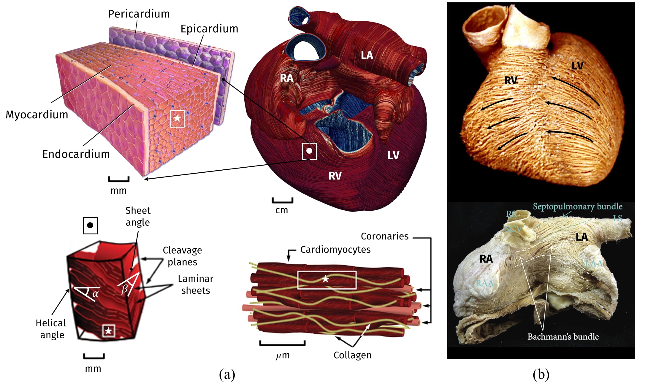
Figure 2: (a) Representation of the multiscale cardiac muscle. (b) Anatomical dissection of myocardial fibers in ventricles (top) and atria (bottom). Images taken and readapted from [54, 55, 56, 57]. Images were available either freely under a Creative Commons Attribution license or have been granted reuse permission by the copyright holder.

Atrial fibers architecture is very different from that of the ventricles, where myofibers are aligned in a regular pattern [18]. Indeed, myofibers in the atria are arranged in individual bundles running along different directions throughout the wall chambers [23, 24]. Preferred orientation of myofibers in the human atria is characterized by multiple overlapping structures, which promote the formation of separate attached bundles [25], as shown in Figure 2.

The cardiac muscular fiber architecture is the backbone of a proper pumping function and has a strong influence on the electric signal propagation throughout the myocardium and also on the mechanical contraction of the muscle [26, 27, 28, 29]. This motivates the need to accurately include fibers orientation in cardiac computational models in order to obtain physically sound results [30, 3, 16].

Due to the difficulty of reconstructing cardiac fibers from medical imaging, different methodologies have been proposed to provide a realistic surrogate of myofibers orientation [31, 21, 32, 33, 34, 35, 36, 37, 38, 39]. Among these, atlas-based methods map and project a detailed fiber field, previously reconstructed on an atlas, on the geometry of interest, exploiting imaging or histological data [21, 34, 39]. However, these methods require complex registration algorithms and their results depend on the original atlas data upon which they have been built.

Alternative strategies for generating myofiber orientations are the Rule-Based Methods [40, 41, 42, 35, 36, 37, 32, 3]. RBM describe fiber orientations with mathematically sound rules based on histological and imaging observations and only require information about the myocardial geometry [18]. These methods parametrize the transmural and apico-basal directions in the entire myocardium in order to assign orthotropic (longitudinal, transversal and normal) myofibers [3].

A particular class of RBM, which relies on the solution of Laplace boundary-value problems, is known as s, addressed in [31, 32, 33] and recently analyzed under a unified mathematical formulation [3]. LDRBMs define the transmural and apico-basal directions by taking the gradient of harmonic functions (the potentials) corresponding to suitable Dirichlet boundary conditions. These directions are then properly rotated to match histological observations [18, 21, 20, 23].

This initial release includes a generator for myocardial fibers based on LDRBMs [3], with application to a number of different prototypical and realistic geometries (slab models, left ventricles and left atria).

s

In this section, we briefly recall the LDRBMs that stand behind the myocardial fiber generation. In Section Results and Discussion we will present several examples where we elaborate on how to reproduce and run the algorithms presented hereafter.

This getting started guide presents LDRBMs for (ventricular and spherical) slabs, (based and complete) left ventricular and left atrial geometries. For further details about the LDRBMs presented here see also [3].

The following common steps are the building blocks of all LDRBMs.

1. Labelled mesh:

Provide a labelled volumetric mesh of the domain $\Omega$ to define specific partition of the boundary $\partial\Omega$ as

$$\partial\Omega=\Gamma_{\mathrm{epi}}\cup\Gamma_{\mathrm{endo}}\cup\Gamma_{\mathrm{base}}\cup\Gamma_{\mathrm{apex}},$$

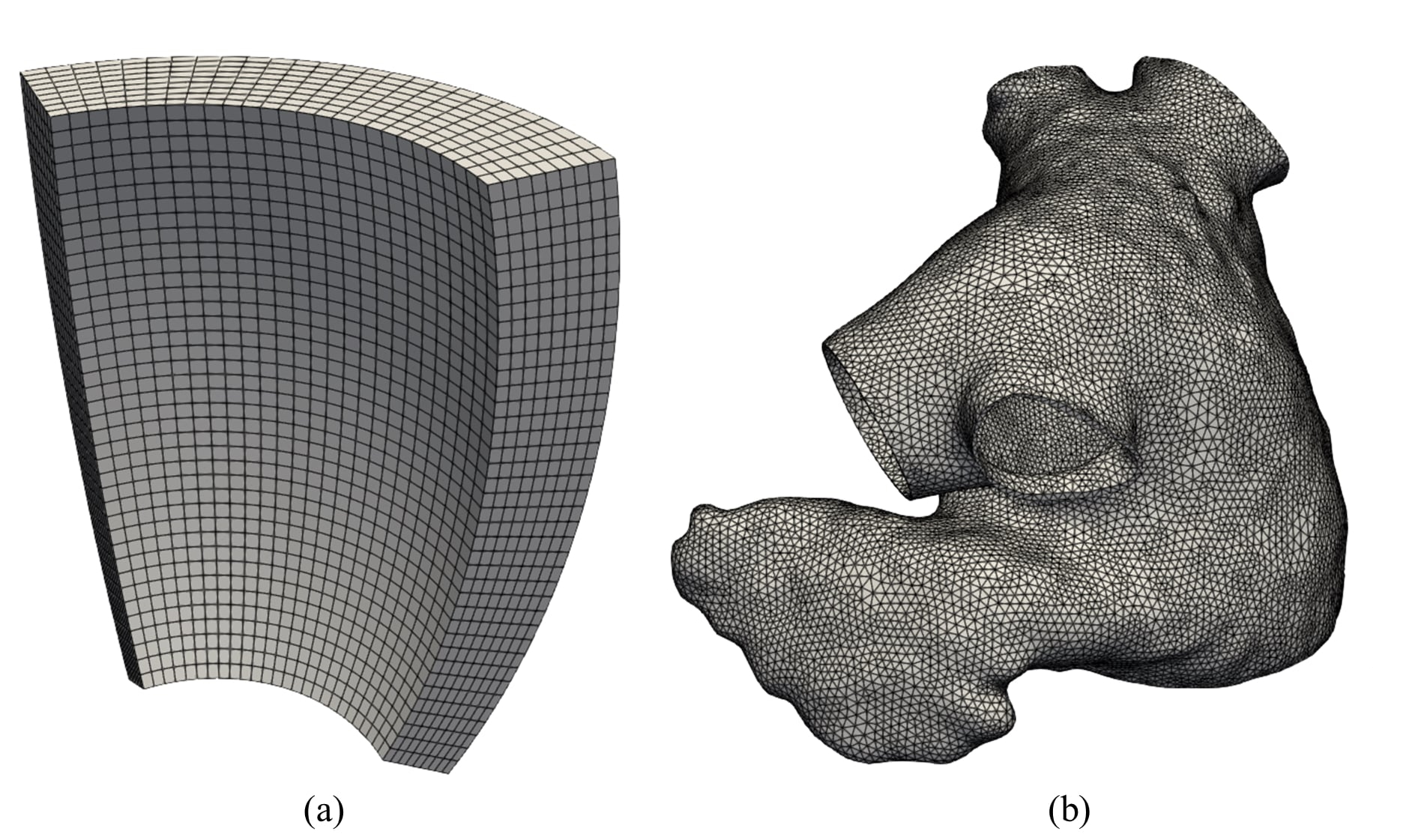
Figure 3: (a) Hexahedral mesh of a ventricular slab. (b) Tetrahedral mesh of a realistic left atrium [38].

where $\Gamma_{\mathrm{endo}}$ is the endocardium, $\Gamma_{\mathrm{epi}}$ is the epicardium, $\Gamma_{\mathrm{base}}$ is the basal plane and $\Gamma_{\mathrm{apex}}$ is the apex, which are demarcated through proper surface labels included in the input mesh. life^x is designed to support both hexahedral and tetrahedral labelled meshes in the widely used *.msh format, see Figure 3. This type of mesh can be generated by a variety of mesh generation software (e.g. gmsh, netgen, vmtk and meshtools). Otherwise, other mesh-format types can be converted in *.msh using for example the open-source library meshio.

Epicardium and endocardium:

for the ventricular slab geometry $\Gamma_{\mathrm{endo}}$ and $\Gamma_{\mathrm{epi}}$ are the lateral walls of the slab, see Figures 4(a); for the spherical slab, the ventricular and atrial geometries $\Gamma_{\mathrm{endo}}$ and $\Gamma_{\mathrm{epi}}$ are the internal and external surfaces, see Figures 4(b-f).

Basal plane and apex:

for the ventricular slab geometry $\Gamma_{\mathrm{base}}$ and $\Gamma_{\mathrm{apex}}$ are the top and bottom surfaces, respectively (see Figure 4(a)); for the spherical slab, $\Gamma_{\mathrm{base}}$ and $\Gamma_{\mathrm{apex}}$ are selected as the north and south pole points of the epicardial sphere (see Figure 4(b)); for the based ventricular geometry $\Gamma_{\mathrm{base}}$ is an artificial basal plane located well below the cardiac valves (see Figure 4(d)), while for the complete ventricular geometry $\Gamma_{\mathrm{base}}$ is split into $\Gamma_{\mathrm{mv}}$ and $\Gamma_{\mathrm{av}}$, representing the mitral and aortic valve rings, respectively (see Figure 4(e)); for the ventricular geometries $\Gamma_{\mathrm{apex}}$ is selected as the epicardial point furthest from the ventricular base (see Figures 4(d-e)); for the atrial geometry $\Gamma_{\mathrm{base}}$ is the mitral valve ring and $\Gamma_{\mathrm{apex}}$ represents the apex of the left atrial appendage (see Figures 4(c-f));

Atrial pulmonary rings:

the atrial geometry type also requires the definition of the boundary labels for the left $\Gamma_{\mathrm{lpv}}$ and right $\Gamma_{\mathrm{rpv}}$ pulmonary vein rings, see Figures 4(c-f).

2. Transmural direction:

A transmural distance $\phi$ is defined to compute the distance of the epicardium from the endocardium, by means of the following Laplace-Dirichlet (LD) problem:

$$[left=\empheqlbrace]\begin{aligned} -\Delta\phi&=0,&\qquad&{\text{in }}\Omega,\\ \phi&=1,&\qquad&{\text{on }}\Gamma_{\mathrm{epi}},\\ \phi&=0,&\qquad&{\text{on }}\Gamma_{\mathrm{endo}},\\ \nabla\phi\cdot\mathbf{n}&=0,&\qquad&{\text{on }}\partial\Omega\setminus(\Gamma_{\mathrm{endo}}\cup\Gamma_{\mathrm{epi}}).\end{aligned}$$ (1)

Then, the transmural distance gradient $\nabla\phi$ is used to build the unit transmural direction:

$$\widehat{\boldsymbol{e}}_{t}=\frac{\nabla\phi}{\|\nabla\phi\|}.$$

3. Normal direction:

A normal (or apico-basal) direction $\boldsymbol{k}$ (which is directed from the apex towards the base) is introduced and used to build the unit normal direction $\widehat{\boldsymbol{e}}_{n}$:

$$\widehat{\boldsymbol{e}}_{n}=\frac{\boldsymbol{k}-(\boldsymbol{k}\cdot\widehat{\boldsymbol{e}}_{t})\widehat{\boldsymbol{e}}_{t}}{\|\boldsymbol{k}-(\boldsymbol{k}\cdot\widehat{\boldsymbol{e}}_{t})\widehat{\boldsymbol{e}}_{t}\|}.$$

The normal direction $\boldsymbol{k}$ can be computed following one of these approaches (see also Figure 5):

Rossi-Lassila (RL) et al. approach [31]:

$\boldsymbol{k}$ is defined as the vector $\mathbf{n}_{\mathrm{base}}$, i.e. the outward normal to the basal plane, that is $\boldsymbol{k}=\mathbf{n}_{\mathrm{base}}$.

Bayer-Trayanova (BT) et al. approach [32]:

$\boldsymbol{k}$ is the gradient of the solution $\psi$ ($\boldsymbol{k}=\nabla\psi$), which can be obtained by solving the following LD problem:

$$[left=\empheqlbrace]\begin{aligned} -\Delta\psi&=0,&\qquad&{\text{in }}\Omega,\\ \psi&=1,&\qquad&{\text{on }}\Gamma_{\mathrm{base}},\\ \psi&=0,&\qquad&{\text{on }}\Gamma_{\mathrm{apex}},\\ \nabla\psi\cdot\mathbf{n}&=0,&\qquad&{\text{on }}\partial\Omega\setminus(\Gamma_{\mathrm{base}}\cup\Gamma_{\mathrm{apex}}).\end{aligned}$$ (2)

Doste et al. approach [33]:

$\boldsymbol{k}$ is a weighted sum of the apico-basal ($\nabla\psi_{\mathrm{ab}}$) and apico-outflow-tract ($\nabla\psi_{\mathrm{ot}}$) directions, obtained using an interpolation function $w$:

$$\boldsymbol{k}=w\nabla\psi_{\mathrm{ab}}+(1-w)\nabla\psi_{\mathrm{ot}},$$

where $\psi_{\mathrm{ab}}$ and $\psi_{\mathrm{ot}}$ are obtained by solving LD problems in the form of (2) where $\Gamma_{\mathrm{base}}=\Gamma_{\mathrm{mv}}$ (for $\psi_{\mathrm{ab}}$) and $\Gamma_{\mathrm{base}}=\Gamma_{\mathrm{av}}$ (for $\psi_{\mathrm{ot}}$), respectively. Moreover, the interpolation function $w$ is obtained by solving:

$$[left=\empheqlbrace]-\Delta w =0, {\text{in }}\Omega,$$

$$w =1, {\text{on }}\Gamma_{\mathrm{mv}}\cup\Gamma_{\mathrm{apex}},$$

$$w =0, {\text{on }}\Gamma_{\mathrm{av}},$$

$$\nabla w\cdot\mathbf{n} =0, {\text{on }}\partial\Omega\setminus(\Gamma_{\mathrm{av}}\cup\Gamma_{\mathrm{mv}}\cup\Gamma_{\mathrm{apex}}).$$

Piersanti et al. approach [3]:

for each point in $\Omega$, a unique normal direction $\boldsymbol{k}$ is selected among the gradient of several normal directions $\boldsymbol{k}=\nabla\psi_{\mathrm{i}}$ ($\mathrm{i=ab,v,r}$), where $\psi_{\mathrm{i}}$ are obtained by solving the following LD problem

$$[left=\empheqlbrace]\begin{aligned} -\Delta\psi_{\mathrm{i}}&=0,&\qquad&{\text{in }}\Omega,\\ \psi_{\mathrm{i}}&=\chi_{\mathrm{a}},&\qquad&{\text{on }}\Gamma_{\mathrm{a}},\\ \psi_{\mathrm{i}}&=\chi_{\mathrm{b}},&\qquad&{\text{on }}\Gamma_{\mathrm{b}},\\ \nabla\psi_{i}\cdot\mathbf{n}&=0,&\qquad&{\text{on }}\partial\Omega\setminus(\Gamma_{\mathrm{a}}\cup\Gamma_{\mathrm{b}}).\end{aligned}$$ (3)

Please refer to [3] for further details about the selection procedure for $\boldsymbol{k}$ and the specific choices of $\chi_{\mathrm{a}}$, $\chi_{\mathrm{b}}$, $\Gamma_{\mathrm{a}}$ and $\Gamma_{\mathrm{b}}$ in problem (2) made for $\psi_{\mathrm{i}}$ ($i=\mathrm{ab},\mathrm{v},\mathrm{r}$).

The BT approach is used in the ventricular and spherical slab geometry types, see also Figure 5(a). The BT and RL approaches can be adopted in the based ventricular geometry (by setting either Algorithm type equal to BT or RL in the parameter file, respectively), while the Doste approach is used in the complete ventricular geometry, see also Figure 5(b). Finally, the Piersanti approach is employed for the atrial geometry, see also Figure 5(c).

4. Local coordinate system:

For each point of the domain an orthonormal local coordinate axial system is defined by $\widehat{\boldsymbol{e}}_{t}$, $\widehat{\boldsymbol{e}}_{n}$ and the unit longitudinal direction $\widehat{\boldsymbol{e}}_{l}$ (orthogonal to the previous ones), as shown in Figure 6:

$$Q=\left[\widehat{\boldsymbol{e}}_{l},\widehat{\boldsymbol{e}}_{n},\widehat{\boldsymbol{e}}_{t}\right]=\left\{\begin{aligned} \widehat{\boldsymbol{e}}_{t}&=\frac{\nabla\phi}{\|\nabla\phi\|},\\ \widehat{\boldsymbol{e}}_{n}&=\frac{\boldsymbol{k}-(\boldsymbol{k}\cdot\widehat{\boldsymbol{e}}_{t})\widehat{\boldsymbol{e}}_{t}}{\|\boldsymbol{k}-(\boldsymbol{k}\cdot\widehat{\boldsymbol{e}}_{t})\widehat{\boldsymbol{e}}_{t}\|},\\ \widehat{\boldsymbol{e}}_{l}&=\widehat{\boldsymbol{e}}_{n}\times\widehat{\boldsymbol{e}}_{t}.\end{aligned}\right.$$ (4)

5. Axis rotation:

The reference frame is rotated with the purpose of defining the myofibers orientation: $\boldsymbol{f}$ the fiber direction, $\boldsymbol{n}$ the sheet-normal direction and $\boldsymbol{s}$ the sheet direction. Specifically, $\widehat{\boldsymbol{e}}_{l}$ rotates counter-clockwise around $\widehat{\boldsymbol{e}}_{t}$ by the helical angle $\alpha$, whereas the transmural direction $\widehat{\boldsymbol{e}}_{t}$ is rotated counter-clockwise around $\widehat{\boldsymbol{e}}_{l}$ by the sheetlet angle $\beta$, see Figure 6:

$$\left[\widehat{\boldsymbol{e}}_{l},\widehat{\boldsymbol{e}}_{n},\widehat{\boldsymbol{e}}_{t}\right]\longrightarrow\left[\boldsymbol{f},\boldsymbol{n},\boldsymbol{s}\right],$$

The rotation angles follow the linear relationships:

$$\alpha(\phi)=\alpha_{\mathrm{endo}}(1-\phi)+\alpha_{\mathrm{epi}}\phi,\qquad\beta(\phi)=\beta_{\mathrm{endo}}(1-\phi)+\beta_{\mathrm{epi}}\phi,$$

where $\alpha_{\mathrm{endo}}$, $\alpha_{\mathrm{epi}}$, $\beta_{\mathrm{endo}}$, $\beta_{\mathrm{epi}}$ are suitable helical and sheetlet rotation angles on the epicardium and endocardium (specifying in the parameter file alpha epi, alpha endo, beta epi, beta endo). Moreover, for the complete ventricular geometry it is possible to set specific fiber and sheet angle rotations in the outflow tract (OT) region (i.e. around the aortic valve ring) by specifying alpha epi OT, alpha endo OT, beta epi OT, beta endo OT). Finally, for the atrial geometry type, no transmural variation in the myofibers direction is prescribed and the three unit directions correspond to the final myofibers directions $[\widehat{\boldsymbol{e}}_{l},\widehat{\boldsymbol{e}}_{n},\widehat{\boldsymbol{e}}_{t}]=[\boldsymbol{f},\boldsymbol{n},\boldsymbol{s}]$.

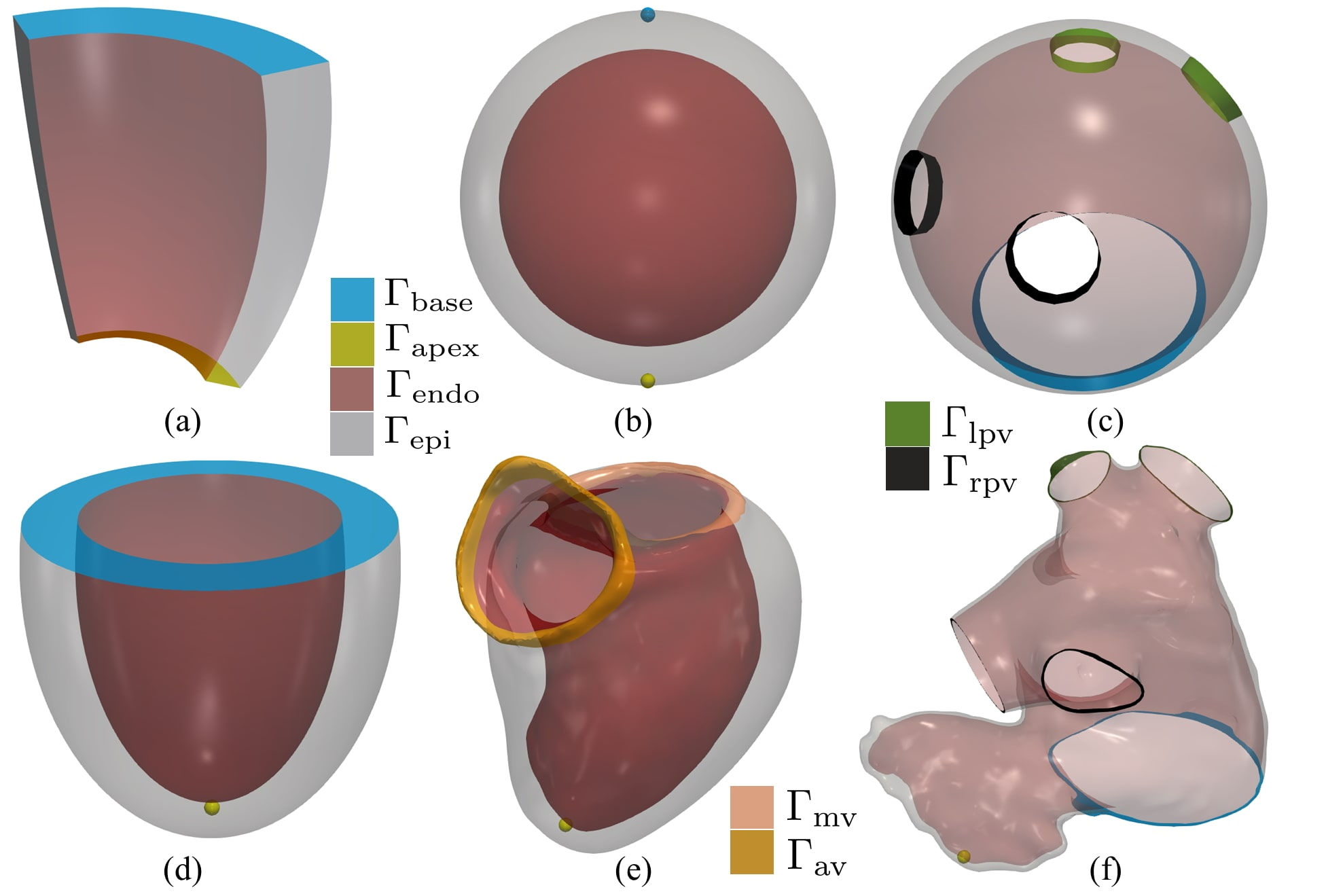
Figure 4: Labelled meshes. (a) Ventricular slab. (b) Spherical slab. (c) Idealized left atrium. (d) Idealized based left ventricle. (e) Realistic complete left ventricle. (f) Realistic left atrium. $\Gamma_{\mathrm{base}}$ denotes the basal plane, $\Gamma_{\mathrm{apex}}$ the apex, $\Gamma_{\mathrm{endo}}$ the endocardium, $\Gamma_{\mathrm{epi}}$ the epicardium, $\Gamma_{\mathrm{lpv}}$, $\Gamma_{\mathrm{rpv}}$ the left (right) pulmonary veins, respectively.

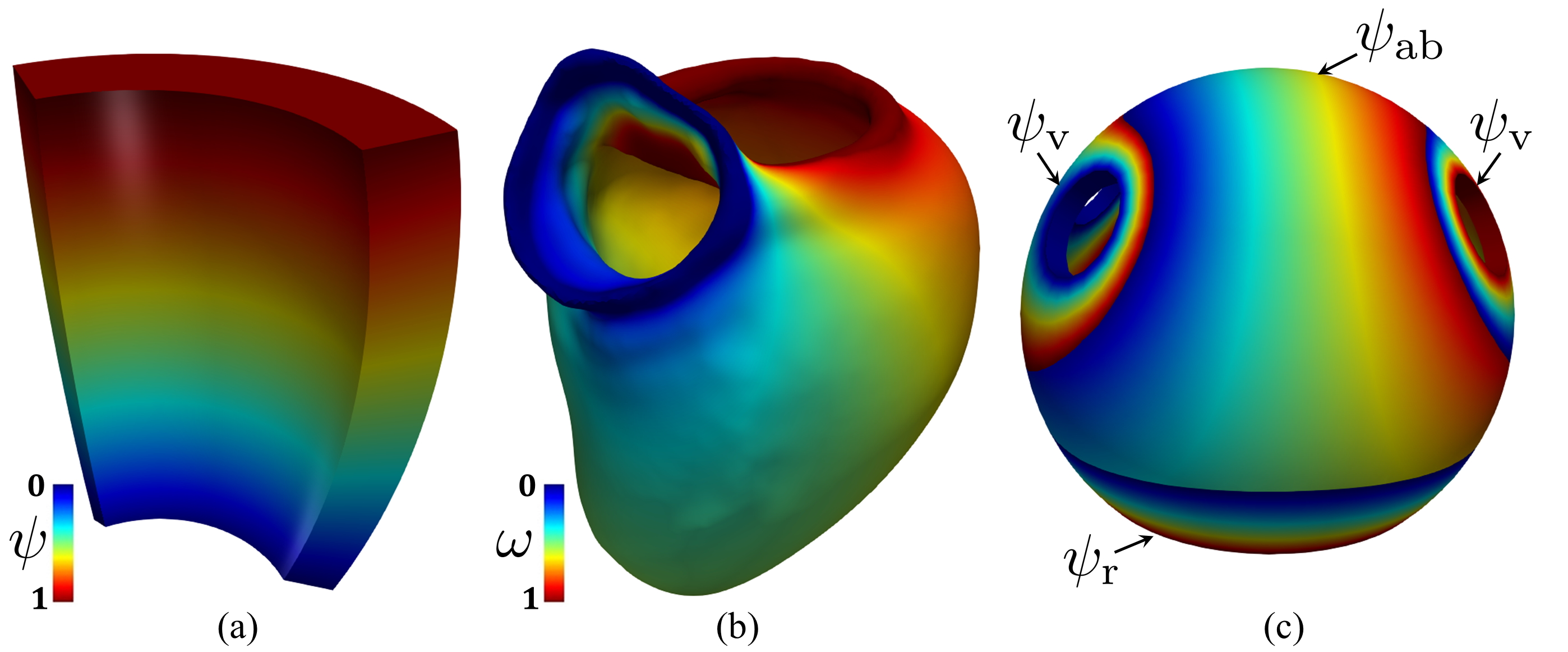
Figure 5: Different types of normal distances: (a) Bayer-Trayanova et al. approach [32]. (b) Doste et al. approach [33]. (c) Piersanti et al. approach [3].

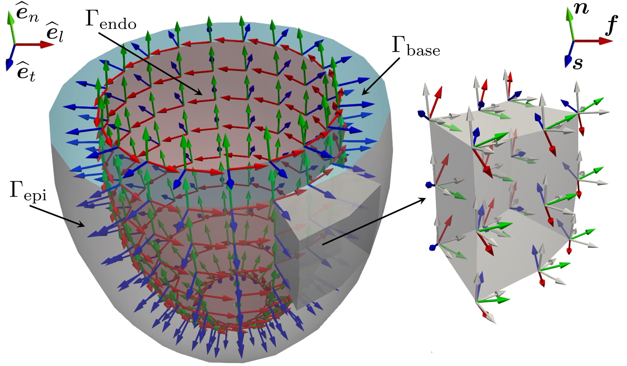
Figure 6: Representation of the local coordinate system employed by a LDRBM for an idealized ventricular domain. Only directions on the endocardium $\Gamma_{\mathrm{endo}}$ are represented. In blue: unit transmural direction, $\widehat{\boldsymbol{e}}_{t}$. In green: unit normal direction, $\widehat{\boldsymbol{e}}_{n}$. In red: unit longitudinal direction, $\widehat{\boldsymbol{e}}_{l}$. Right: zoom on a slab of the left ventricular myocardium showing the three final myofibers orientations $\boldsymbol{f}$, $\boldsymbol{s}$ and $\boldsymbol{n}$.

In order to represent the fiber architecture, LDRBMs use the gradient of specific intra-chamber distances, by means of harmonic problems, combined with a precise definition of boundary sections where boundary conditions are prescribed. This strategy makes the fibers less open to subjective variability. On the other hand, the myofiber orientations could be adapted to a patient-specific setting by simply changing the parameters involved in LDRBMs (e.g. the helical and sheetlet angles $\alpha$ and $\beta$). Therefore, unlike other RBMs requiring manual or semi-automatic interventions, LDRBMs can be easily applied to any arbitrary patient-specific geometry [3].

Comparison to existing software

Several packages have been developed and are available in the framework of cardiac fibers generation.

Meshtools [43] is a comand-line tool designed to automate image-based mesh generation and manipulate tasks in cardiac modeling workflows, such as operations on label fields and/or geometric features; it integrates seamlessly with the openCARP ecosystem [44]; the algorithms supported are only for left ventricular geometries and of BT type. KIT-IBT-LDRB_Fibers is a MATLAB tool for generating left and bi-ventricular fibers; the original BT algorithm was adapted to eliminate a discontinuity in the fiber field in correspondence of the free walls and to yield a fiber rotation that is directly proportional to the transmural Laplace solution (approximately linear across the wall) [45]. CARDIO SUITE for GIMIAS includes tools for patient-specific modelling that allow to generate the FE meshes required for the simulations and to build additional structures such as fiber orientation [46]; at the time of writing and to the best of our knowledge, the latest version was released in 2016. SimCardio is advertised as the only fully open-source software package providing a complete pipeline from medical image data segmentation to patient specific blood flow simulation and analysis; its module svFSI supports specifying distributed fiber and sheet direction generated by BT-like rule-based algorithms.

Poisson interpolation algorithms [35] have inspired the implementation of fiber generation packages, despite being generally more computationaly demanding than, e.g., RL or BT algorithms [31]. This class of methods has been implemented in Cardiac Chaste, which supports automatic generation of mathematical model for fiber orientation associated with both idealized and anatomically-based geometry meshes [47], and in BeatIt, which is to our knowledge the only publicly available software which natively supports the generation of fiber architectures also for atrial geometries [48].

Compared to the software described above, the strengths of life^x reside in its user-friendly interface and in its generality, by supporting either idealized and realistic, (left) ventricular and atrial geometries and for each of them the user can selected one of the different state-of-the-art algorithms described in Section  ‣ Background. Finally, life^x offers a seamless integration with many other core models (specifically cardiac electrophysiology, mechanics and electromechanics) for modeling the cardiac function from single-chamber to whole-heart simulations which will be targeted by future releases.

Implementation

In this section we introduce technical specifications of life^x as well as a thorough documentation of the user interface exposed. The users will be guided from downloading it to running a full simulation of the algorithms presented in Section  ‣ Background.

Technical specifications

Here we specify the package content, copyright and licensing information and software and hardware specifications required by the present life^x release.

Package content

The fiber generation module of life^x is delivered in binary form as an AppImage executable.

This provides a universal package for x86-64 Linux operating systems, without the need to deliver different distribution-specific versions. From the user’s perspective, this implies an effortless download-then-run process, without having to manually take care of installing the proper system dependencies required.

Once the source code will be made publicly accessible, a standard build-from-source procedure with automatic installers will be available to make the dependencies setup tailored to the specific hardware of HPC facilities or cloud platforms.

License and third-party software

This work is copyrighted by the life^x authors and licensed under the Creative Commons Attribution Non-Commercial No-Derivatives 4.0 International License.

life^x makes use of third-party libraries. Please note that such libraries are copyrighted by their respective authors (independent of the life^x authors) and are covered by various permissive licenses.

The third-party software bundled with (in binary form), required by, copied, modified or explicitly used in life^x include the following packages:

Boost:

its modules Filesystem and Math are used for manipulating files/directories and for advanced mathematical functions and interpolators, respectively;

deal.II:

it provides support to mesh handling, assembling and solving Finite Element problems (with a main support to third-party libraries as PETSc and Trilinos for linear algebra data structures and solvers) and to input/output functionalities;

VTK:

it is used for importing external surface or volume input data and coefficients appearing in the mathematical formulation.

Some of the packages listed above, as stated by their respective authors, rely on additional third-party dependencies that may also be bundled (in binary form) with life^x, although not used directly. These dependencies include: ADOL-C, ARPACK-NG, BLACS, Eigen, FFTW, GLPK, HDF5, HYPRE, METIS, MUMPS, NetCDF, OpenBLAS, ParMETIS, ScaLAPACK, Scotch, SuiteSparse, SuperLU, oneTBB, p4est.

The libraries listed above are all free software and, as such, they place few restrictions on their use. However, different terms may hold. Please refer to the content of the folder doc/licenses/ for more information on license and copyright statements for these packages.

Finally, an MPI installation (such as OpenMPI or MPICH) may also be required to successfully run life^x executables in parallel.

Software and hardware requirements

As an AppImage, this life^x release has been built on Debian Buster (the current oldstable version) following the “Build on old systems, run on newer systems” paradigm.

Therefore, it is expected to run on (virtually) any recent enough x86-64 Linux distribution, assuming that glibc version 2.28 or higher is installed.

Quick start guide: running a life^x executable

The following steps are required in order to run a life^x executable.

Download and install

First, download and extract the life^x release archive available at https://doi.org/10.5281/zenodo.5810268. Then :

1. open a terminal;

2. move to the directory containing the
   lifex_fiber_generation-1.4.0-x86_64.AppImage file:

   ⬇

   cd /path/to/lifex/

3. make the AppImage executable:

   ⬇

   chmod +x lifex_fiber_generation-1.4.0-x86_64.AppImage

4. lifex_fiber_generation-1.4.0-x86_64.AppImage is now ready to be executed:

   ⬇

   ./lifex_fiber_generation-1.4.0-x86_64.AppImage [ARGS]...

Root permissions are not required. Please note that, in order for the above procedure to succeed, AppImage relies upon the userspace filesystem framework FUSE which is assumed to be installed on your system. In case of errors, please try with the following commands:

⬇

./lifex_fiber_generation-1.4.0-x86_64.AppImage \

--appimage-extract

squashfs-root/usr/bin/lifex_fiber_generation [ARGS]...

or refer to the AppImage troubleshooting guide.

Step 0 - Set the parameter file

Each life^x application or example (including also the fiber generation executable described in Section Download and install) defines a set of parameters that are required in order to be run. They involve problem-specific parameters (such as constitutive relations, geometry, time interval, boundary conditions, …) as well as numerical parameters (types of linear/non-linear solvers, tolerances, maximum number of iterations, …) or output-related options.

In case an application has sub-dependencies (such as a linear solver), also the related parameters are included (typically in a proper subsection).

Every application comes with a set of command line options, which can be printed using the -h (or --help) flag:

⬇

./executable_name -h

The first step before running an executable is to generate the parameter file(s) containing all the default parameter values. This is done via the -g (or --generate-params) flag:

⬇

./executable_name -g

that by default generates a parameter file named after the executable, in .prm format.

By default, only parameters considered standard are printed. The parameter file verbosity can be decreased or increased by passing an optional flag minimal or full to the -g flag, respectively:

⬇

./executable_name -g minimal

The parameter basename to generate can be customized with the -f (or --params-filename) option:

⬇

./executable_name -g -f custom_param_file.ext

Absolute or relative paths can be specified.

At user’s option, in order to guarantee a flexible interface to external file processing tools, the parameter file extension ext can be chosen among three different interchangeable file formats prm, json or xml, from the most human-readable to the most machine-readable.

As an example, the three parameter files listed in Listings 1, 2 and 3 are semantically equivalent.

We highlight that, following with the design of the ParameterHandler class of deal.II, each parameter is provided with:

• a given pattern, specifying the parameter type (e.g. boolean, integer, floating-point number, string, list, …) and, whenever relevant, a range of admissible values (pattern description);

• a default value, printed in the parameter file upon generation and implicitly assumed if the user omits a custom value;

• the actual value, possibly overriding the default one;

• a documentation string;

• a global index.

All of these features, combined to a runtime check for the correctness of each parameter, make the code syntactically and semantically robust with respect to possible errors or typos introduced unintentionally.

⬇

# Listing of Parameters

# ---------------------

subsection Fiber generation

subsection Mesh and space discretization

# Specify whether the input mesh has hexahedral or

# tetrahedral elements. Available options are: Hex | Tet.

set Element type = Hex

# Number of global mesh refinement steps applied to the initial grid (Hex only).

set Number of refinements = 0

subsection File

# Mesh file.

set Filename =

# Mesh scaling factor: 1e-3 => from [mm] to [m].

set Scaling factor = 1e-3

end

end

subsection Output

# Enable/disable output.

set Enable output = true

# Output file.

set Filename = fibers

end

end

Listing 1: PRM parameter file format.

⬇

{

"Fiber_20generation": {

"Mesh_20and_20space_20discretization": {

"File": {

"Filename": {

"value": "",

"default_value": "",

"documentation": "Mesh file.",

"pattern": "0",

"pattern_description": "[FileName (Type: input)]"

},

"Scaling_20factor": {

"value": "1",

"default_value": "1e-3",

"documentation": "Mesh scaling factor: 1e-3 => from [mm] to [m].",

"pattern": "1",

"pattern_description": "[Double 0...MAX_DOUBLE (inclusive)]"

}

},

"Element_20type": {

"value": "Hex",

"default_value": "Hex",

"documentation": "Specify whether the input mesh has hexahedral or tetrahedral elements. Available options are: Hex | Tet.",

"pattern": "2",

"pattern_description": "[Selection Hex|Tet ]"

},

"Number_20of_20refinements": {

"value": "0",

"default_value": "0",

"documentation": "Number of global mesh refinement steps applied to the initial grid (Hex only).",

"pattern": "3",

"pattern_description": "[Integer range 0...2147483647 (inclusive)]"

}

},

"Output": {

"Enable_20output": {

"value": "true",

"default_value": "true",

"documentation": "Enable\/disable output.",

"pattern": "4",

"pattern_description": "[Bool]"

},

"Filename": {

"value": "fibers",

"default_value": "fibers",

"documentation": "Output file.",

"pattern": "5",

"pattern_description": "[FileName (Type: output)]"

}

}

}

}

Listing 2: JSON parameter file format.

⬇

<?xml version="1.0" encoding="utf-8"?>

<ParameterHandler>

<Fiber_20generation>

<Mesh_20and_20space_20discretization>

<File>

<Filename>

<value/>

<default_value/>

<documentation>Mesh file.</documentation>

<pattern>0</pattern>

<pattern_description>[FileName (Type: input)]</pattern_description>

</Filename>

<Scaling_20factor>

<value>1</value>

<default_value>1</default_value>

<documentation>Mesh scaling factor: 1e-3 =&gt; from [mm] to [m].</documentation>

<pattern>1</pattern>

<pattern_description>[Double 0...MAX_DOUBLE (inclusive)]</pattern_description>

</Scaling_20factor>

</File>

<Element_20type>

<value>Hex</value>

<default_value>Hex</default_value>

<documentation>Specify whether the input mesh has hexahedral or tetrahedral elements. Available options are: Hex | Tet.</documentation>

<pattern>2</pattern>

<pattern_description>[Selection Hex|Tet ]</pattern_description>

</Element_20type>

<Number_20of_20refinements>

<value>0</value>

<default_value>0</default_value>

<documentation>Number of global mesh refinement steps applied to the initial grid (Hex only).</documentation>

<pattern>3</pattern>

<pattern_description>[Integer range 0...2147483647 (inclusive)]</pattern_description>

</Number_20of_20refinements>

</Mesh_20and_20space_20discretization>

<Output>

<Enable_20output>

<value>true</value>

<default_value>true</default_value>

<documentation>Enable/disable output.</documentation>

<pattern>4</pattern>

<pattern_description>[Bool]</pattern_description>

</Enable_20output>

<Filename>

<value>fibers</value>

<default_value>fibers</default_value>

<documentation>Output file.</documentation>

<pattern>5</pattern>

<pattern_description>[FileName (Type: output)]</pattern_description>

</Filename>

</Output>

</Fiber_20generation>

</ParameterHandler>

Listing 3: XML parameter file format.

Once generated, the user can modify, copy, move or rename the parameter file depending on their needs.

Step 1 - Run

To run an executable, the -g flag has simply to be omitted whereas the -f option is used to specify the parameter file to be read (as opposed to written, in generation mode), e.g.:

⬇

./executable_name -f custom_param_file.ext [option...]

If no -f flag is provided, a file named executable_name.prm is assumed to be available in the directory where the executable is run from.

The path to the directory where all the app output files will be saved to can be selected via the -o (or --output-directory) flag:

⬇

./executable_name -o ./results/

If the specified directory does not already exist, it will be created. By default, the current working directory is used.

Absolute or relative paths can be specified for both the input parameter file and the output directory.

Parallel run

To run an app in parallel, use the mpirun or mpiexec wrapper commands (which may vary depending on the MPI implementation available on your machine) e.g.:

⬇

mpirun -n <N_PROCS> ./executable_name [option...]

where <N_PROCS> is the desired number of parallel processes to run on.

As a rule of thumb, 10000 to 100000 degrees of freedom per process should lead to the best performance.

Dry run and parameter file conversion

Upon running, a parameter log file is automatically generated in the output directory, that can be used later to retrieve which parameters had been used for a specific run.

By default, log_params.ext will be used as its filename. This can be changed via the -l (or --log-file) flag, e.g.:

⬇

./executable_name -l my_log_file.ext [option...]

The extension is not mandatory: if unspecified, the same extension as the input parameter file will be used.

If the dry run option is enabled via the -d (or --dry-run) flag, the execution terminates right after the parameter log file generation. This has a two-fold purpose:

1. checking the correctness of the parameters being declared and parsed before running the actual simulation (if any of the parameters does not match the specified pattern or has a wrong name or has not been declared in a given subsection then a runtime exception is thrown);

2. converting a parameter file between two different formats/extensions. For example, the following command converts input.xml to
   output.json:

   ⬇

   ./executable_name -f input.xml -d -l output.json [option...]

Results and Discussion

The LDRBMs described in Section  ‣ Background have been applied to a set of idealized or realistic test cases, namely ventricular and spherical slabs, based and complete left ventricular and left atrial geometries.

This section presents the results obtained, as well as a possible pipeline for reproducing such test cases, consisting of the following steps:

1. setting up input data (e.g. generating or importing computational meshes);

2. setting up the parameter files associated with a given simulation scenario and running the corresponding simulation;

3. post-processing the solution and visualizing the output.

A mesh sensitivity analysis has been performed and reported in Section Mesh sensitivity and validation.

Input data

Additional input data (scripts, meshes and parameter files) associated with the guided examples described below can be downloaded from the release archive https://doi.org/10.5281/zenodo.5810268.

In this getting started guide, we provide different ready-to-use meshes, namely

• a set of four idealized geometries consisting of a ventricular slab, a spherical slab, an idealized based left ventricle and an idealized left atrium, see Figures 4(a-d);

• two realistic geometries composed by a left ventricle and a left atrium, see Figures 4(e-f).

The idealized meshes have been generated using the built-in CAD engine of gmsh, an open-source 3D FE mesh generator, starting from the corresponding gmsh geometrical models (represented by *.geo files, also provided) defined using their boundary representation, where a volume is bounded by a set of surfaces. For details about the geometrical definition of a model geometry we refer to the online documentation of gmsh.

In order to perform the mesh generation, starting from the geometrical files provided in this tutorial, the following command can be run in a terminal:

⬇

gmsh geometry.geo -clscale s -o mesh.msh -save

where geometry.geo is the geometrical file model, mesh.msh is the output mesh file, which will be provided as an input to a life^x app, and s $\in(0,1]$ is the mesh element size factor. To produce a coarser (finer) mesh the clscale factor can be reduced (increased).

The realistic left ventricle and left atrium have been produced starting from the open-source meshes adopted in [38] (for the left atrium) and in [49] (for the left ventricle) and using the Vascular Modelling Toolkit (vmtk) software [50] along with the semi-automatic meshing tools recently proposed in [51].

All the characteristic informations of the ready-to-use meshes, above described, are reported in Table 1.

Geometry	Type	$\text{h}_{\text{min}}\,\text{[mm]}$	$\text{h}_{\text{avg}}\,\text{[mm]}$	$\text{h}_{\text{max}}\,\text{[mm]}$	#elements	#vertices	Quality
Ventricular slab	Hex	4.74	5.95	6.73	988	1400	1.69
Ventricular slab	Tet	3.10	6.76	8.71	2439	762	2.91
Spherical slab	Tet	1.96	3.46	4.70	18455	4924	2.46
Idealized left atrium	Tet	2.78	3.43	4.15	10039	3387	2.36
Idealized left ventricle	Tet	1.71	3.53	4.93	74488	16567	3.27
Realistic left ventricle	Tet	0.51	1.17	1.67	1885227	330703	2.80
Realistic left atrium	Tet	0.15	1.00	1.76	112994	33297	4.23

Table 1: Mesh information regarding the ready-to-use meshes presented in this work. In particular the mesh quality is computed selecting the edge ratio option in the ParaView mesh quality filter.

Generating fibers

Parameter files for fiber generation are characterized by a common section named Mesh and space discretization. Select Element type = Tet for tetrahedral meshes or Element type = Hex for hexahedral meshes. Finally, specify in FE space degree the degree of the (piecewise continuous) polynomial FE space used to solve the LD problems described above. Finally, we remark that life^x internally treats all physical quantities as if they are provided in International System of Units (SI): therefore, a Scaling factor can be set in order to convert the input mesh from a given unit of measurement (e.g. if the mesh coordinates are provided in millimeters then Scaling factor must be set equal to 1e-3).

The Geometry type parameters enables to specify the kind of geometry provided in input, in order to apply the proper LDRBM algorithm among the ones described above. Once specified, parameters related to the specific algorithm and geometry will be parsed from a subsection named after the value of Geometry type.

All parameters missing from the parameter file will take their default value, which is hard-coded.

⬇

subsection Mesh and space discretization

set Element type = Tet

set FE space degree = 1

set Geometry type = Slab

subsection File

set Filename = /path/to/mesh/slab.msh

set Scaling factor = 1e-3

end

end

Slab fibers

Specify Geometry type = Slab to prescribe fibers in slab geometries and the path of the input mesh file in Filename.

Ventricular slab

For a ventricular slab geometry Sphere slab = false must be set. Specify the label for the top (Tags base up) and bottom (Tags base down) surfaces of the slab, as well as the epicardium (Tags epi) and endocardium (Tags endo) ones. Finally, prescribe the helical and sheetlet rotation angles at the epicardium and endocardium using the corresponding alpha epi, alpha endo, beta epi, beta endo parameters.

⬇

subsection Slab

set Sphere slab = false

set Tags base up = 50

set Tags base down = 60

set Tags epi = 10

set Tags endo = 20

set alpha epi = -60

set alpha endo = 60

set beta epi = 45

set beta endo = -45

end

Spherical slab

For a spherical slab geometry set Sphere slab = true. Specify the epicardial coordinates $(x,y,z)$ of the north (North pole) and south (South pole) poles of the sphere of the slab, and the labels of the endocardium (Tags endo) and epicardium (Tags epi). Finally, prescribe the helical and sheetlet rotation angles at the epicardium and endocardium in alpha epi, alpha endo, beta epi, beta endo. A fiber architecture for the sphere slab with radial fiber $\boldsymbol{f}$ can be prescribed by setting in the parameter file Sphere with radial fibers = true. This consists of exchanging the sheet direction $\boldsymbol{s}$ with the fiber direction $\boldsymbol{f}$. Instead, a tangential (to the epicardial and endocardial surfaces) fiber field $\boldsymbol{f}$ is assigned when Sphere with radial fibers = false.

⬇

subsection Slab

set Sphere slab = true

set Sphere with radial fibers = true

set North pole = 0 0 0.025

set South pole = 0 0 -0.025

set Tags epi = 10

set Tags endo = 20

set alpha epi = 0

set alpha endo = 0

set beta epi = 0

set beta endo = 0

end

Left ventricular fibers

Specify Geometry type = Left ventricle to prescribe fibers in a based left ventricular geometry, or Geometry type = Left ventricle complete to prescribe fibers in complete left ventricular geometry. Other mesh-related parameters have the same meaning as described above.

⬇

subsection Mesh and space discretization

set Element type = Tet

set FE space degree = 1

set Geometry type = Left ventricle complete

subsection File

set Filename = /path/to/mesh/ventricle.msh

set Scaling factor = 1e-3

end

end

Based left ventricle

Specify the labels for the basal plane (Tags base), the epicardium (Tags epi) and endocardium (Tags endo) of the ventricle. Select RL or BT approach in Algorithm type. Prescribe the helical and sheetlet rotation angles at the epicardium and endocardium in alpha epi, alpha endo, beta epi, beta endo. Finally, for the RL approach specify the outward normal vector to the basal plane in Normal to base, while for the BT approach prescribe the apex epicardial coordinates $(x,y,z)$ (Apex) of the ventricle.

⬇

subsection Left ventricle

set Tags base = 50

set Tags epi = 10

set Tags endo = 20

set Algorithm type = BT

set alpha epi = -60

set alpha endo = 60

set beta epi = 20

set beta endo = -20

subsection RL

set Normal to base = 0 0 1

end

subsection BT

set Apex = 0 0 0.0601846

end

end

Selecting the RL approach as Algorithm type, this setup can be also exploited in bi-ventricular geometries (not included in the example meshes). In this case, the mesh must have two additional surface labels in the right ventricular endocardium: one delimiting the part facing to the septum (e.g. 15) and the other for the remaining part (e.g. 25). In this way, it is sufficient to set Tags endo as the two endocardial labels (excluding the right septum) and Tags epi as the epicardial label and the right endocardial septum label. Further detail on this approach can be found in [3].

⬇

subsection Left ventricle

...

set Tags epi = 10, 15

set Tags endo = 20, 25

set Algorithm type = RL

...

end

Complete left ventricle

Specify the labels for the mitral (Tags MV) and aortic (Tags AV) valve rings, the epicardium (Tags epi) and endocardium (Tags endo) of the ventricle. Prescribe the apex epicardial coordinates $(x,y,z)$ in Apex. Finally, define the helical and sheetlet rotation angles at the epicardium and endocardium in alpha epi, alpha endo, beta epi, beta endo. A specific helical and sheetlet rotation angles around the outflow tract of the left ventricle (i.e. the mitral valve ring) can be specified by setting alpha epi OT, alpha endo OT, beta epi OT, beta endo OT.

⬇

subsection Left ventricle complete

set Tags MV = 50

set Tags AV = 60

set Tags epi = 10

set Tags endo = 20

set Apex = 0.0692 0.0710 0.3522

set alpha epi = -60

set alpha endo = 60

set beta epi = 20

set beta endo = -20

set alpha epi OT = 0

set alpha endo OT = 90

set beta epi OT = 0

set beta endo OT = 0

end

Left atrial fibers

Specify Geometry type = Left atrium to prescribe fibers in a left atrial geometry. Other mesh-related parameters have the same meaning as described above.

⬇

subsection Mesh and space discretization

set Element type = Tet

set FE space degree = 1

set Geometry type = Left atrium

subsection File

set Filename = /path/to/mesh/atrium.msh

set Scaling factor = 1e-3

end

end

Idealized left atrium

Select Appendage = false to prescribe fibers in the hollow sphere geometry. Specify the labels for the mitral valve ring (Tags MV), the right (Tags RPV) and left (Tags LPV) pulmonary veins rings, the epicardium (Tags epi) and endocardium (Tags endo) of the idealized atrium. Finally, select the dimension of the atrial bundles: Tau bundle MV for the mitral valve bundle; Tau bundle LPV and Tau bundle RPV for the left and right pulmonary valves rings bundle.

⬇

subsection Left atrium

set Appendage = false

set Tags epi = 30

set Tags endo = 10

set Tags RPV = 20

set Tags LPV = 50

set Tags MV = 40

set Tau bundle MV = 0.65

set Tau bundle LPV = 0.85

set Tau bundle RPV = 0.15

end

Realistic left atrium

Select Appendage = true to prescribe fibers in a realistic left atrial geometry. Specify the labels for the mitral valve ring (Tags MV), the right (Tags RPV) and left (Tags LPV) pulmonary veins rings, the epicardium (Tags epi) and endocardium (Tags endo) of the idealized atrium. Prescribe in Apex the epicardial coordinates $(x,y,z)$ for the apex of the atrial appendage. Finally, select the dimension of the atrial bundles: for the mitral valve bundle Tau bundle MV; for the left and right pulmonary valves rings bundle Tau bundle LPV and Tau bundle RPV, respectively.

⬇

subsection Left atrium

set Appendage = true

set Apex = 83.868 16.369 45.989

set Tags epi = 30

set Tags endo = 10

set Tags RPV = 20

set Tags LPV = 50

set Tags MV = 40

set Tau bundle MV = 0.60

set Tau bundle LPV = 0.90

set Tau bundle RPV = 0.10

end

Output and visualization

To enable the output select Enable output = true and specify the corresponding output filename in Filename. This will produce a XDMF schema file named output_filename.xdmf (wrapped around a same-named HDF5 output file output_filename.h5) that can be visualized in ParaView, an open-source multi-platform data analysis and visualization application. Specifically, the streamtracer and the tube filters of ParaView can be applied in sequence to visualize the fiber fields, such as the one shown in Figure 7.

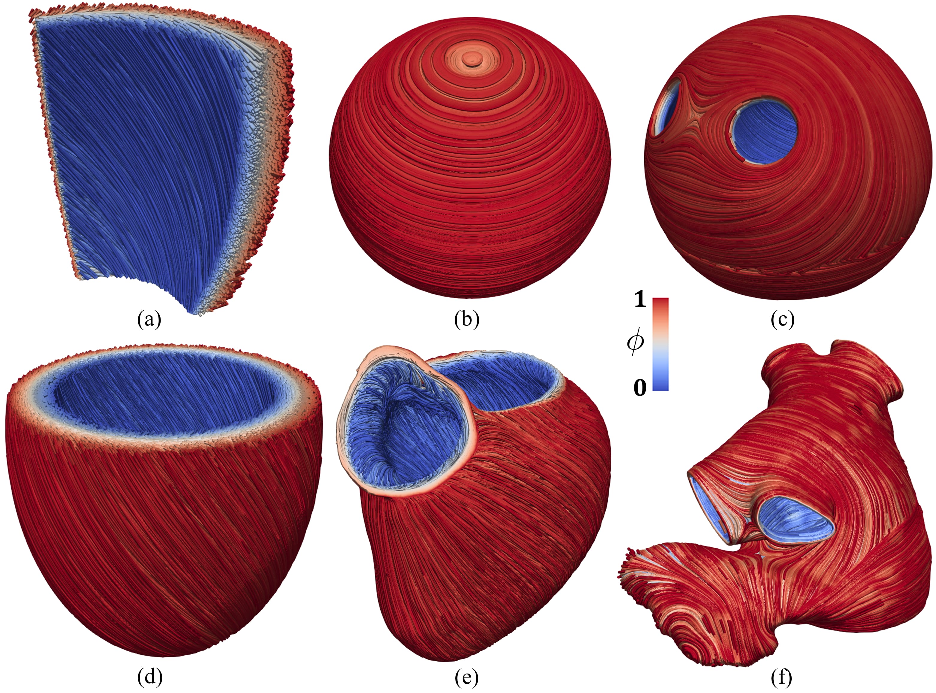
Figure 7: Fiber field $\boldsymbol{f}$ visualized as streamlines. (a) Ventricular slab. (b) Spherical slab with circumferential fibers. (c) Idealized left atrium. (d) Idealized based left ventricle. (e) Realistic complete left ventricle. (f) Realistic left atrium.

⬇

subsection Output

set Enable output = true

set Filename = fibers

end

Moreover, the HDF5 file format guarantees that the output can easily be further post-processed, not only for visualization purposes but rather to be fed as an input to more sophisticated computational pipelines.

Mesh sensitivity and validation

The robustness of the algorithms presented above is confirmed by performing a mesh sensitivity analysis. Specifically, we consider the ventricular slab geometry shown in Figure 4(a) and two related sets of discretization with hexahedral and with tetrahedral elements, respectively. For each of the two element types, we run the fiber generation algorithm (see Section Ventricular slab) for four decreasing mesh sizes $h_{1}>h_{2}>h_{3}>h_{4}$.

As the fibers field is orthonormalized, the difference between two numerical solutions is only due to the orientation angle. This allows us to define an error estimate as:

$$\Delta_{\theta}^{i}=\left|\arccos\left(\mathbf{f}_{0}^{i}\cdot\mathbf{f}_{0}^{4}\right)\right|,\ i=1,2,3,$$

where $\mathbf{f}_{0}^{i}$ is the fiber field computed on the mesh with size $h_{i}$ and the results on the finest mesh with size $h_{4}$ are considered as a reference solution.

i	$h\,\text{[mm]}$	#dofs	$\displaystyle\operatorname*{avg}_{\Omega}\Delta_{\theta}^{i}\,[{}^{\circ}]$	$\displaystyle\max_{\Omega}\Delta_{\theta}^{i}\,[{}^{\circ}]$
1	5.95	1400	0.62	6.33
2	3.00	9477	0.24	4.54
3	1.50	69377	0.08	2.40
4	0.75	530145	—	—

Table 2: Mesh sensitivity analysis for hexahedral elements.

i	$h\,\text{[mm]}$	#dofs	$\displaystyle\operatorname*{avg}_{\Omega}\Delta_{\theta}^{i}\,[{}^{\circ}]$	$\displaystyle\max_{\Omega}\Delta_{\theta}^{i}\,[{}^{\circ}]$
1	6.76	762	1.35	7.85
2	3.53	3989	0.50	5.57
3	1.76	25661	0.19	4.28
4	0.88	179338	—	—

Table 3: Mesh sensitivity analysis for tetrahedral elements.

We show the error distribution in the whole domain in Figure 8, while Tables 2 and 3 report the average and maximum errors for the hexahedral and the tetrahedral meshes, respectively. We determine both an average and a maximum error smaller than 8^∘ even for the coarsest mesh. These values are very small and, in particular, much smaller than the physiological fibers dispersion angle [52].

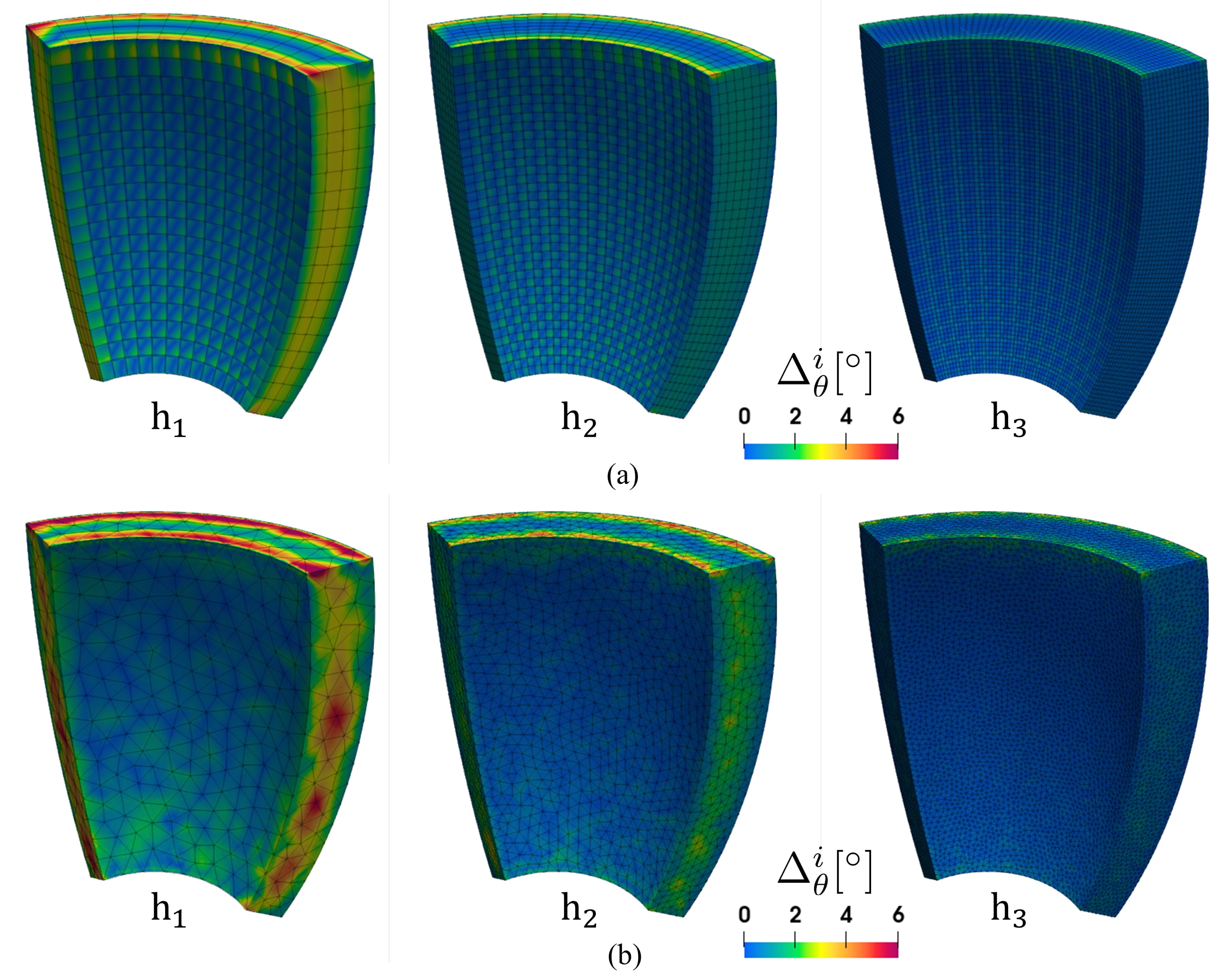
Figure 8: Mesh sensitivity analysis performed on the ventricular slab geometry and three different mesh sizes $h_{1},h_{2},h_{3}$. (a) Hexahedral meshes. (b) Tetrahedral meshes.

The interest of accurately reconstructing a fiber orientation field consists of providing it as an input to more sophisticated computational models, such as for cardiac electrophysiology and electromechanics. As the dynamics of such physical models demands for a high resolution in both time and space [3, 16, 53], the LDRBM algorithms are typically run on fine meshes. Therefore, the impact of possible numerical errors due to the mesh size is to be considered negligible, as confirmed by the small errors presented above.

The proposed LDRBMs have been validated in [3], where the fiber orientation field computed numerically provided a satisfactory match to histological data.

Furthermore, the anisotropic nature of the fiber orientation strongly influences the electrophysiological, mechanical and electromechanical cardiac function. Therefore, an indirect way to validate the fiber field provided by LDRBMs is to compute quantitative indices or biomarkers in such kind of simulations.

Matching quantitative indices in a physiological range is only possible when the fiber reconstruction algorithm is accurate enough: this is shown in [3] for the whole-heart electrophysiology, in [16] for the ventricular electromechanics, and in [53] for the whole-heart electromechanics.

Future developments

As anticipated in Section Background, the development of life^x has been initially oriented towards a heart module incorporating packages for the simulation of cardiac electrophysiology, mechanics, electromechanics and blood fluid dynamics models.

In the near future, the deployment of life^x will follow two lines:

• more modules will be successively published in binary form, starting from an advanced solver for cardiac electrophysiology and other solvers for the cardiac function;

• in the meantime, the source code associated with life^x core and with previous binary releases will be gradually made publicly available under an open-source license.

In the long run, also modules unrelated to the cardiac function are expected to be included within life^x.

Conclusions

life^x is intended to provide the scientific community with an integrated FE framework for exploring many physiological and pathological scenarios using in silico experiments for the whole-heart cardiac function, boosting both the user and developer experience without sacrificing its computational efficiency and universality.

We believe that this software release provides the scientific community with an invaluable tool for in silico scenario analyses of myofibers orientation; such a tool supports either idealized and realistic, (left) ventricular and atrial geometries. It also offers a seamless integration of LDRBMs into more sophisticated computational pipelines involving other core models – such as electrophysiology, mechanics and electromechanics – for the cardiac function, in a wide range of settings covering from single-chamber to whole-heart simulations.

The content of this initial release is published on the official website https://lifex.gitlab.io/: we encourage users to interact with the life^x development community via the issue tracker of our public website repository. Any curiosity, question, bug report or suggestion is welcome!

News and announcements about life^x will be posted to the official website https://lifex.gitlab.io/. Stay tuned!

Availability and requirements

Project name: life^x
Project home page: https://lifex.gitlab.io/
Operating system(s): Linux (x86-64)
Programming language: C++
Other requirements: glibc version 2.28 or higher
License: CC BY-NC-ND 4.0
Any restrictions to use by non-academics: no additional restriction.

List of abbreviations

FE

Finite Element

BT

Bayer-Trayanova

RL

Rossi-Lassila

HPC

High Performance Computing

LD

Laplace-Dirichlet

RBM

Rule-Based Method

LDRBM

Laplace-Dirichlet Rule-Based Method

SI

International System of Units

References

- [1] Quarteroni, A., Dede’, L., Manzoni, A., Vergara, C.: Mathematical Modelling of the Human Cardiovascular System: Data, Numerical Approximation, Clinical Applications. Cambridge Monographs on Applied and Computational Mathematics, vol. 33 (2019). doi:10.1017/9781108616096
- [2] Quarteroni, A., Lassila, T., Rossi, S., Ruiz-Baier, R.: Integrated heart—coupling multiscale and multiphysics models for the simulation of the cardiac function. Computer Methods in Applied Mechanics and Engineering 314, 345–407 (2017). doi:10.1016/j.cma.2016.05.031. Special Issue on Biological Systems Dedicated to William S. Klug
- [3] Piersanti, R., Africa, P.C., Fedele, M., Vergara, C., Dede’, L., Corno, A.F., Quarteroni, A.: Modeling cardiac muscle fibers in ventricular and atrial electrophysiology simulations. Computer Methods in Applied Mechanics and Engineering 373, 113468 (2021)
- [4] Salvador, M., Fedele, M., Africa, P.C., Sung, E., Dede’, L., Prakosa, A., Chrispin, J., Trayanova, N., Quarteroni, A.: Electromechanical modeling of human ventricles with ischemic cardiomyopathy: numerical simulations in sinus rhythm and under arrhythmia. Computers in Biology and Medicine 136, 104674 (2021). doi:10.1016/j.compbiomed.2021.104674
- [5] Salvador, M., Regazzoni, F., Pagani, S., Dede’, L., Trayanova, N., Quarteroni, A.: The role of mechano-electric feedbacks and hemodynamic coupling in scar-related ventricular tachycardia. Computers in Biology and Medicine, 105203 (2022)
- [6] ten Tusscher, K.H.W.J., Panfilov, A.V.: Alternans and spiral breakup in a human ventricular tissue model. American Journal of Physiology-Heart and Circulatory Physiology 291(3), 1088–1100 (2006). doi:10.1152/ajpheart.00109.2006. PMID: 16565318
- [7] Courtemanche, M., Ramirez, R.J., Nattel, S.: Ionic mechanisms underlying human atrial action potential properties: insights from a mathematical model. American Journal of Physiology-Heart and Circulatory Physiology 275(1), 301–321 (1998). doi:10.1152/ajpheart.1998.275.1.H301. PMID: 9688927
- [8] Arndt, D., Bangerth, W., Blais, B., Fehling, M., Gassmöller, R., Heister, T., Heltai, L., Köcher, U., Kronbichler, M., Maier, M., Munch, P., Pelteret, J.P., Proell, S., Konrad, S., Turcksin, B., Wells, D., Zhang, J.: The deal.II library, version 9.3. Journal of Numerical Mathematics 29(3), 171–186 (2021). doi:10.1515/jnma-2021-0081
- [9] Regazzoni, F., Salvador, M., Africa, P.C., Fedele, M., Dede’, L., Quarteroni, A.: A cardiac electromechanical model coupled with a lumped-parameter model for closed-loop blood circulation. Journal of Computational Physics, 111083 (2022)
- [10] Regazzoni, F., Quarteroni, A.: Accelerating the convergence to a limit cycle in 3d cardiac electromechanical simulations through a data-driven 0d emulator. Computers in Biology and Medicine 135, 104641 (2021). doi:10.1016/j.compbiomed.2021.104641
- [11] Zingaro, A., Fumagalli, I., Fedele, M., Africa, P.C., Dede’, L., Quarteroni, A., Corno, A.F.: A geometric multiscale model for the numerical simulation of blood flow in the human left heart. Discrete and Continuous Dynamical Systems - S 15(8), 2391–2427 (2022). doi:10.3934/dcdss.2022052
- [12] Bucelli, M., Dede’, L., Quarteroni, A., Vergara, C.: Partitioned and monolithic algorithms for the numerical solution of cardiac fluid-structure interaction. MOX Report (2021). https://www.mate.polimi.it/biblioteca/add/qmox/78-2021.pdf
- [13] Fumagalli, I., Vitullo, P., Scrofani, R., Vergara, C.: Image-based computational hemodynamics analysis of systolic obstruction in hypertrophic cardiomyopathy. medRxiv (2021). doi:10.1101/2021.06.02.21258207
- [14] Stella, S., Vergara, C., Maines, M., Catanzariti, D., Africa, P.C., Demattè, C., Centonze, M., Nobile, F., Del Greco, M., Quarteroni, A.: Integration of activation maps of epicardial veins in computational cardiac electrophysiology. Computers in Biology and Medicine 127, 104047 (2020). doi:10.1016/j.compbiomed.2020.104047
- [15] Dede’, L., Regazzoni, F., Vergara, C., Zunino, P., Guglielmo, M., Scrofani, R., Fusini, L., Cogliati, C., Pontone, G., Quarteroni, A.: Modeling the cardiac response to hemodynamic changes associated with covid-19: a computational study. Mathematical Biosciences and Engineering 18(4), 3364–3383 (2021)
- [16] Piersanti, R., Regazzoni, F., Salvador, M., Corno, A.F., Dede’, L., Vergara, C., Quarteroni, A.: 3d-0d closed-loop model for the simulation of cardiac biventricular electromechanics. Computer Methods in Applied Mechanics and Engineering 391, 114607 (2022). doi:10.1016/j.cma.2022.114607
- [17] Quarteroni, A., Lassila, T., Rossi, S., Ruiz-Baier, R.: Integrated Heart-Coupling multiscale and multiphysics models for the simulation of the cardiac function. Computer Methods in Applied Mechanics and Engineering 314, 345–407 (2017)
- [18] Streeter Jr, D.D., Spotnitz, H.M., Patel, D.P., Ross Jr, J., Sonnenblick, E.H.: Fiber orientation in the canine left ventricle during diastole and systole. Circulation Research 24(3), 339–347 (1969)
- [19] LeGrice, I.J., Smaill, B.H., Chai, L.Z., Edgar, S.G., Gavin, J.B., Hunter, P.J.: Laminar structure of the heart: ventricular myocyte arrangement and connective tissue architecture in the dog. American Journal of Physiology-Heart and Circulatory Physiology 269(2), 571–582 (1995)
- [20] Greenbaum, R.A., Ho, S.Y., Gibson, D.G., Becker, A.E., Anderson, R.H.: Left ventricular fibre architecture in man. Heart 45(3), 248–263 (1981)
- [21] Lombaert, H., Peyrat, J., Croisille, P., Rapacchi, S., Fanton, L., Cheriet, F., Clarysse, P., Magnin, I., Delingette, H., Ayache, N.: Human atlas of the cardiac fiber architecture: study on a healthy population. IEEE Transactions on Medical Imaging 31(7), 1436–1447 (2012)
- [22] Toussaint, N., Stoeck, C.T., Schaeffter, T., Kozerke, S., Sermesant, M., Batchelor, P.G.: In vivo human cardiac fibre architecture estimation using shape-based diffusion tensor processing. Medical Image Analysis 17(8), 1243–1255 (2013)
- [23] Ho, S.Y., Anderson, R.H., Sánchez-Quintana, D.: Atrial structure and fibres: morphologic bases of atrial conduction. Cardiovascular Research 54, 325–336 (2002)
- [24] Ho, S.Y., Sánchez-Quintana, D.: The importance of atrial structure and fibers. Clinical Anatomy: The Official Journal of the American Association of Clinical Anatomists and the British Association of Clinical Anatomists 22, 52–63 (2009)
- [25] D. Sánchez-Quintana, D., Pizarro, G., López-Mínguez, J.R., Ho, S.Y., Cabrera, J.A.: Standardized review of atrial anatomy for cardiac electrophysiologists. Journal of Cardiovascular Translational Research 6, 124–144 (2013)
- [26] Roberts, D.E., Hersh, L.T., Scher, A.M.: Influence of cardiac fiber orientation on wavefront voltage, conduction velocity, and tissue resistivity in the dog. Circulation Research 44(5), 701–712 (1979)
- [27] Punske, B.B., Taccardi, B., Steadman, B., Ershler, P.R., England, A., Valencik, M.L., McDonald, J.A., Litwin, S.E.: Effect of fiber orientation on propagation: electrical mapping of genetically altered mouse hearts. Journal of Electrocardiology 38(4), 40–44 (2005)
- [28] Eriksson, T.S.E., Prassl, A.J., Plank, G., Holzapfel, G.A.: Influence of myocardial fiber/sheet orientations on left ventricular mechanical contraction. Mathematics and Mechanics of Solids 18(6), 592–606 (2013)
- [29] Palit, A., Bhudia, S.K., Arvanitis, T.N., Turley, G.A., Williams, M.A.: Computational modelling of left-ventricular diastolic mechanics: Effect of fibre orientation and right-ventricle topology. Journal of Biomechanics 48(4), 604–612 (2015)
- [30] Guan, D., Yao, J., Luo, X., Gao, H.: Effect of myofibre architecture on ventricular pump function by using a neonatal porcine heart model: from DT-MRI to rule-based methods. Royal Society Open Science 7(4), 191655 (2020)
- [31] Rossi, S., Lassila, T., Ruiz-Baier, R., Sequeira, A., Quarteroni, A.: Thermodynamically consistent orthotropic activation model capturing ventricular systolic wall thickening in cardiac electromechanics. European Journal of Mechanics-A/Solids 48, 129–142 (2014)
- [32] Bayer, J.D., Blake, R.C., Plank, G., Trayanova, N.: A novel rule-based algorithm for assigning myocardial fiber orientation to computational heart models. Annals of Biomedical Engineering 40(10), 2243–2254 (2012)
- [33] Doste, R., Soto-Iglesias, D., Bernardino, G., Alcaine, A., Sebastian, R., Giffard-Roisin, S., Sermesant, M., Berruezo, A., Sanchez-Quintana, D., Camara, O.: A rule-based method to model myocardial fiber orientation in cardiac biventricular geometries with outflow tracts. International Journal for Numerical Methods in Biomedical Engineering 35(4), 3185 (2019)
- [34] Hoermann, J.M., Pfaller, M.R., Avena, L., Bertoglio, C., Wall, W.A.: Automatic mapping of atrial fiber orientations for patient-specific modeling of cardiac electromechanics using image registration. International Journal for Numerical Methods in Biomedical Engineering 35(6), 3190 (2019)
- [35] Wong, J., Kuhl, E.: Generating fibre orientation maps in human heart models using poisson interpolation. Computer methods in biomechanics and biomedical engineering 17(11), 1217–1226 (2014)
- [36] Krueger, M.W., Schmidt, V., Tobón, C., Weber, F.M., Lorenz, C., Keller, D.U.J., Barschdorf, H., Burdumy, M., Neher, P., Plank, G., et al.: Modeling atrial fiber orientation in patient-specific geometries: a semi-automatic rule-based approach. In: International Conference on Functional Imaging and Modeling of the Heart, pp. 223–232 (2011)
- [37] Ferrer, A., Sebastián, R., Sánchez-Quintana, D., Rodríguez, J.F., Godoy, E.J., Martínez, L., Saiz, J.: Detailed anatomical and electrophysiological models of human atria and torso for the simulation of atrial activation. PloS One 10(11), 0141573 (2015)
- [38] Fastl, T.E., Tobon-Gomez, C., Crozier, A., Whitaker, J., Rajani, R., McCarthy, K.P., Sanchez-Quintana, D., Ho, S.Y., O’Neill, M.D., Plank, G., et al.: Personalized computational modeling of left atrial geometry and transmural myofiber architecture. Medical Image Analysis (2018)
- [39] Roney, C.H., Bendikas, R., Pashakhanloo, F., Corrado, C., Vigmond, E.J., McVeigh, E.R., Trayanova, N.A., Niederer, S.A.: Constructing a human atrial fibre atlas. Annals of Biomedical Engineering (2020)
- [40] Beyar, R., Sideman, S.: A computer study of the left ventricular performance based on fiber structure, sarcomere dynamics, and transmural electrical propagation velocity. Circulation Research 55(3), 358–375 (1984)
- [41] Potse, M., Dubé, B., Richer, J., Vinet, A., Gulrajani, R.M.: A comparison of monodomain and bidomain reaction-diffusion models for action potential propagation in the human heart. IEEE Transactions on Biomedical Engineering 53(12), 2425–2435 (2006)
- [42] Nielsen, P., Le Grice, I.J., Smaill, B.H., Hunter, P.J.: Mathematical model of geometry and fibrous structure of the heart. American Journal of Physiology-Heart and Circulatory Physiology 260(4), 1365–1378 (1991)
- [43] Neic, A., Gsell, M.A.F., Karabelas, E., Prassl, A.J., Plank, G.: Automating image-based mesh generation and manipulation tasks in cardiac modeling workflows using meshtool. SoftwareX 11, 100454 (2020). doi:10.1016/j.softx.2020.100454
- [44] Plank, G., Loewe, A., Neic, A., Augustin, C., Huang, Y.-L., Gsell, M.A.F., Elias Karabelas, J.S. Mark Nothstein, Prassl, A.J., Seemann, G., Vigmond, E.J.: The openCARP simulation environment for cardiac electrophysiology. Computer Methods and Programs in Biomedicine 208, 106223 (2021). doi:10.1016/j.cmpb.2021.106223
- [45] Kovacheva, E., Gerach, T., Schuler, S., Ochs, M., Dössel, O., Loewe, A.: Causes of altered ventricular mechanics in hypertrophic cardiomyopathy: an in-silico study. BioMedical Engineering OnLine 20(1), 1–28 (2021)
- [46] Larrabide, I., Omedas, P., Martelli, Y., Planes, X., Nieber, M., Moya, J.A., Butakoff, C., Sebastián, R., Camara, O., Craene, M.D., et al.: Gimias: an open source framework for efficient development of research tools and clinical prototypes. In: International Conference on Functional Imaging and Modeling of the Heart, pp. 417–426 (2009). Springer
- [47] Cooper, F.R., Baker, R.E., Bernabeu, M.O., Bordas, R., Bowler, L., Bueno-Orovio, A., Byrne, H.M., Carapella, V., Cardone-Noott, L., Cooper, J., et al.: Chaste: cancer, heart and soft tissue environment. Journal of Open Source Software (2020)
- [48] Rossi, S., Gaeta, S., Griffith, B.E., Henriquez, C.S.: Muscle thickness and curvature influence atrial conduction velocities. Frontiers in physiology, 1344 (2018)
- [49] Strocchi, M., Augustin, C.M., Gsell, M.A.F., Karabelas, E., Neic, A., Gillette, K., Razeghi, O., Prassl, A.J., Vigmond, E.J., Behar, J.M., Gould, J., Sidhu, B., Rinaldi, C.A., Bishop, M.J., Plank, G., Niederer, S.A.: A publicly available virtual cohort of four-chamber heart meshes for cardiac electro-mechanics simulations. PLOS ONE 15, 1–26 (2020). doi:10.1371/journal.pone.0235145
- [50] Antiga, L., Steinman, D.A.: The vascular modeling toolkit (2008)
- [51] Fedele, M., Quarteroni, A.: Polygonal surface processing and mesh generation tools for the numerical simulation of the cardiac function. International Journal for Numerical Methods in Biomedical Engineering 37(4), 3435 (2021)
- [52] Guan, D., Zhuan, X., Holmes, W., Luo, X., Gao, H.: Modelling of fibre dispersion and its effects on cardiac mechanics from diastole to systole. Journal of Engineering Mathematics 128(1), 1–24 (2021)
- [53] Fedele, M., Piersanti, R., Regazzoni, F., Salvador, M., Africa, P.C., Bucelli, M., Zingaro, A., Dede’, L., Quarteroni, A.: A comprehensive and biophysically detailed computational model of the whole human heart electromechanics. arXiv (2022). doi:10.48550/ARXIV.2207.12460
- [54] Chabiniok, R., Wang, V.Y., Hadjicharalambous, M., Asner, L., Lee, J., Sermesant, M., Kuhl, E., Young, A.A., Moireau, P., Nash, M.P., et al.: Multiphysics and multiscale modelling, data–model fusion and integration of organ physiology in the clinic: ventricular cardiac mechanics. Interface Focus 6(2), 20150083 (2016)
- [55] Anderson, R.H., Niederer, P.F., Sanchez-Quintana, D., Stephenson, R.S., Agger, P.: How are the cardiomyocytes aggregated together within the walls of the left ventricular cone? Journal of Anatomy 235(4), 697–705 (2019)
- [56] Sánchez-Quintana, D., López-Mínguez, J.R., Macías, Y., Cabrera, J.A., Saremi, F.: Left atrial anatomy relevant to catheter ablation. Cardiology Research and Practice 2014 (2014)
- [57] Blausen.com staff: Medical gallery of Blausen Medical 2014. WikiJournal of Medicine (2014). https://en.wikiversity.org/wiki/WikiJournal_of_Medicine/Medical_gallery_of_Blausen_Medical_2014