Deformed Butler-Volmer Models for Convex Semilogarithmic Current-Overpotential Profiles of Li-ion Batteries

Abstract

The Butler-Volmer (BV) equation links the current flux crossing an electrochemical interface to the electric potential drop across it with the assumption of Arrhenius kinetics and the Boltzmann factor. Applying the semilogarithmic Tafel analysis in which the logarithm of current is plotted vs. the overpotential one expects straight lines from which the fundamental reaction rate of the kinetic process can be computed. However, some Li-ion battery data, which is the focus here, show nonlinear convex profiles that cannot be adequately fitted with the standard BV model. We propose instead two deformed BV models for the analysis of such types of behaviors constructed from the superposition of cells exhibiting only local equilibrium and thus giving rise to the power-law $q$-exponential and $\kappa$-exponential functions. Non-Boltzmann distributions have been successfully employed for the modeling of a wide spectrum of physical systems in nonequilibrium situations, but not yet for batteries. We verify the validity of the deformed BV models on experimental data obtained from LiFePO4 and Li-O2 batteries.

UOS]Dept. of Sustainable and Renewable Energy Engineering, University of Sharjah, Sharjah, P.O. Box 27272, United Arab Emirates Center for Advanced Materials Research, Research Institute of Sciences and Engineering, University of Sharjah, Sharjah,, P.O. Box 27272, United Arab Emirates FIU]Dept. of Mechanical and Materials Engineering, Florida International University, Miami, FL33174, United States UOS]Dept. of Applied Physics and Astronomy, University of Sharjah, PO Box 27272, Sharjah, United Arab Emirates FIU]Dept. of Mechanical and Materials Engineering, Florida International University, Miami, FL33174, United States

1 Introduction

Chemical-to-electrical or electrical-to-chemical energy conversion in electrochemical energy devices and systems such as batteries and fuel cells or in electrodeposition and electrolysis require the presence of two phases in contact with each other. Generally there is an electron-conducting phase but ionic insulator on the one hand, and an ionic conductor but electric insulator on the other hand. The phases can be solid, liquid or gas. At the inter-phase boundary or interface, which should be thought of as a physical and not a mathematical plane, chemical reactions accompanied with charge carriers transfer from one phase to another take place. Understanding and properly modeling the measurements carried out on such systems is important for many applications including renewable energy technologies with energy storage, electric vehicles, smart grids, and corrosion prevention ¹. In particular, it is important and useful to describe the system-level relationship between the electrical current flowing through an electrode, or charge dynamics with time, and the potential difference between the electrode itself and a point in the bulk electrolyte. Several approaches have been proposed to model kinetic rate behavior. The macroscopic phenomenological Butler–Volmer (BV) model is the de facto mathematical model used for describing the simultaneous anodic reaction (oxidation) and cathodic reaction (reduction) on the same electrode surface ². Microscopic theories, including Marcus, Marcus-Hush-Chidsey (MHC) and their extensions are also powerful in describing electron transfer kinetics in both directions with physically-tractable quantities ^{3, 4}. However, the main limitation for the widespread use of Marcus-type theories is that the rate has no simple closed-form expression. It is defined in terms on indefinite integral over Fermi-Dirac distribution function for which different computational algorithms have been proposed with different levels of accuracy and computational costs ⁵. Our focus here is on the BV model.

The BV equation can be derived from different approaches including the kinetic law of mass action ⁶, non-equilibrium thermodynamics ², principle of thermal activation process ⁷, and also from first principles ⁸, but here we present the derivation from transition state theory ⁹. From Arrhenius kinetics, it is observed that the natural logarithm of the reaction rate $k$ and the reciprocal of the absolute temperature $T$ are linearly related according to:

$$\frac{\partial\ln(k)}{\partial(1/T)}=-\frac{E_{a}}{R}$$ (1)

where $R$ is the universal gas constant and $E_{a}$ is an experimental/phenomenological activation energy ⁶, which can be thought of as the energy necessary to overcome a certain energy barrier for particles to transition from the well of reactants to the well of products, and thus for the reaction to proceed. Arrhenius’ suggestion that there is a transition state intermediate between reactants and products was central to the development of transition state theory ¹⁰. Let us consider the case of a single-step charge transfer redox reaction of the form:

$$\ce{Ox}+n\ce{e}^{-}\rightleftharpoons\ce{Red}$$ (2)

The forward or oxidation ($\ce{Ox}+n\ce{e}^{-}\rightarrow\ce{Red}$) and backward or reduction ($\ce{Red}\rightarrow\ce{Ox}+n\ce{e}^{-}$) charge transfer reactions can be described by the charge transfer reaction rates $k_{f}$ and $k_{b}$. Their associate forward and backward current densities (per unit surface) crossing the interface are taken to be proportional to the surface concentrations $C_{\text{Ox}}$ and $C_{\text{Red}}$, and can be written as:

$$i_{f}=nFk_{f}C_{\text{Ox}}$$ (3)

$$i_{b}=nFk_{b}C_{\text{Red}}$$ (4)

where $F$ is the Faraday constant. Thus the net current flowing through the electrode is given by the difference ⁶:

$$i=i_{f}-i_{b}=nF(k_{f}C_{\text{Ox}}-k_{b}C_{\text{Red}})$$ (5)

Now by incorporating the expressions for the potential and temperature-dependence of the forward and backward charge transfer reaction rates, which are assumed to follow Arrhenius profiles (with $E_{a}$ taken as a linear function of the potential $\psi$) as:

$$k_{f}=k_{f}^{0}\exp\left(\frac{-\alpha_{\text{Red}}\psi}{RT/F}\right)$$ (6)

$$k_{b}=k_{b}^{0}\exp\left(\frac{\alpha_{\text{Ox}}\psi}{RT/F}\right)$$ (7)

Eq. 5 turns to be:

$${i}={nF}\left\{k_{f}^{0}C_{\ce{Ox}}\exp\left(\frac{-\alpha_{\text{Red}}\psi}{RT/F}\right)-k_{b}^{0}C_{\ce{Red}}\exp\left(\frac{\alpha_{\text{Ox}}\psi}{RT/F}\right)\right\}$$ (8)

This equation is known as the kinetic BV equation for the current-potential relationship with pure charge transfer overpotential. Here, the dimensionless parameters $\alpha_{\ce{Red}}$ and $\alpha_{\ce{Ox}}$ (taking values between 0 and 1 with $\alpha_{\ce{Red}}+\alpha_{\ce{Ox}}=1$) denote the transfer or symmetry factors associated with the oxidation and reduction reactions, respectively, or qualitatively a measure of the ”position” of the transition state ¹¹, $RT/F=V_{th}$ is the thermal voltage, and $\psi$ is the potential of the electrode through which current flows, which is different from the equilibrium potential $\psi_{0}$ established when no current passes through the electrode. The difference $\eta=\psi-\psi_{0}$ is known as the overpotential. Eq. 8 can also be expressed in terms of the current exchange density $i_{0}$ (i.e. when $i_{f}=i_{b}=i_{0}$ which takes place at the equilibrium potential $\psi_{0}$) such that:

$${i}=i_{0}\left\{\exp\left(\frac{-\alpha_{\text{Red}}\eta}{RT/F}\right)-\exp\left(\frac{\alpha_{\text{Ox}}\eta}{RT/F}\right)\right\}$$ (9)

Note that with the use of the dimensionless overpotential scaled to the thermal voltage, $\eta^{*}=\eta/V_{th}$, the dimensionless current $i^{*}=i/i_{0}$, and $\alpha_{\text{Red}}=\alpha$, Eq. 9 can be rewritten as ¹:

$$i^{*}=\exp\left[-\alpha\eta^{*}\right]-\exp\left[(1-\alpha)\eta^{*}\right]$$ (10)

For the particular case of $\alpha=0.5$, which is commonly used for battery modeling, the expression for $i^{*}$ simplifies to:

$$i^{*}=2\sinh(-\eta^{*}/2)$$ (11)

The Tafel technique of plotting $\ln(i^{*})$ versus $\eta^{*}$ gives a straight line of slope $-\alpha$ for $\eta^{*}<0$ and $(1-\alpha)$ for $\eta^{*}>0$ from which the charge transfer rates can be estimated ^{1, 12, 13, 14}.

The validity of the BV model is based on the assumption that the concentration of the reacting species are independent of the current density and the potential, and consequently only pure charge transfer overpotential is involved ⁹. It is also commonly assumed that the transfer coefficient is independent or a weak function of the applied potential and can be considered as constant ¹¹. The surface of the electrode is considered flat and stress-free ⁷. Furthermore, within the BV framework an exponential Boltzmann factor for the reaction rate dependence on the temperature is considered. The Boltzmann factor, which is essentially a comparison between the energy of the molecules and the energy of the barrier when the system is in thermodynamic equilibrium and characterized by a certain temperature, assumes that particles are totally independent, non-interacting and obey the laws of ideal gases ¹⁵. It also assumes that elementary volumes of the system are equiprobable. These assumptions are the basis for Boltzmann-Gibbs (BG) statistical mechanics in which the exponential and Gaussian distributions are those that maximize the BG entropy by virtue of the the Central Limit Theorem (CLT), and ensure the equilibrium state.

However, there are several instances where the semilogarithmic Tafel analysis of $\ln(i^{*})$ versus $\eta^{*}$ does not result in linear profiles, but rather curved plots which is the motivation for this work ^{1, 16, 17, 18, 13, 14}. Focusing on battery materials and devices, curved Tafel plots have been reported for instance by Munakata et al. ¹⁷ in experiments conducted on single (porous) particles of LiFePO4, which is a widely used cathode material for large-scale batteries. The fitting with the BV model with the symmetry factor $\alpha=0.5$ was reasonable enough for a small portion of the voltage-current data only ¹⁷. Viswanathan et al. ¹⁸ reported also highly nonlinear Tafel plots for the discharge of nonaqueous Li-air (or Li-O2) battery. The charging data were less unusual by showing slight nonlinearities in the profiles. Generally speaking, reacting systems we are interested in are actually away from equilibrium and transition from one metastable state to a neighboring state of metastable equilibrium in response to external stimuli ¹⁹. Thus, the assumption of thermodynamic equilibrium is not always appropriate, and the statistics may not necessarily follow BG statistics ^{10, 19, 15}. In fact, for many complex systems at off-equilibrium conditions it is often observed that power-law distributions are most common as it is the case for example with the dissolution reaction of magnesium (or aluminum) in aqueous cupric chloride solution ²⁰. Magnesium (or aluminum) dissolves to form MgCl2 (or AlCl3) and copper precipitates at local reaction rates that can be affected by concentration fluctuations, pitting dissolution and the formation of the Cu layer, which tends to inhibit the reaction itself. Furthermore, the breakdown of the Cu layer because of liberation of hydrogen gas, convective turbulence near the reactive surface, and erosion of underlying metal, increase the local reaction rate at the freshly exposed surfaces. As a result, one observes fluctuations in current and voltage found to follow power-law behavior. ²⁰. Other systems that exhibit power-law statistics are for example the power grid frequency fluctuations ²¹, epidemiology and spreading dynamics of diseases ²², and atomic packing in metallic glasses ²³ to name a few.

The purpose of this contribution is to formulate and study a generalized BV model by incorporating the power-law (i) $q$-exponential function based on Tsallis nonextensive statistics ^{24, 25} and (ii) the $\kappa$-exponential based on Kaniadakis statistics ^{26, 27} instead of the traditional exponential Boltzmann factor based on BG statistics. Such approaches have been proven successful for describing many complex nonequilibrium systems at stationary state that behave like the collective superposition of many subsystems, themselves they follow the BG statistics. These systems usually involve long-range interactions, non-Markovian memory effects and anomalous diffusion for instance. The single Boltzmann factor employed in the BV kinetic model is recovered as a limiting case. We note that the generalization of reaction rate coefficients using the $q$-exponential structure instead of the standard Arrhenius exponential function has been proposed by Niven ²⁸, Bagci ²⁹, Yin et al. ^{30, 31, 32} amongst others ^{33, 34, 35, 36}, but to the best of our knowledge this is the first study on the extension of the BV model using such a framework for analyzing battery data. Furthermore, we are not aware of any studies using the $\kappa$-exponential function to do so.

The rest of the manuscript is organized as follows. In Section 2 we will provide a brief summary of some important deformed functions (mostly deformed exponential functions) and their properties, and formulate the corresponding modified BV expressions. In Section 3 we analyze experimental Lithium batteries results compiled from the literature for which we compare fittings using standard, and $q$- and $\kappa$-deformed BV equations.

2 Theory

We consider the simplified case model of an electrode/electrolyte system with single-step charge transfer redox reaction as described by reaction 2. The global equilibrium of the reacting system, which is driven away from equilibrium, is assumed to be influenced by fluctuations and stochastic events. Such fluctuations can originate for instance from the effects of the non-uniformity of the electrode/electrolyte interfaces, porous and fractal structures, long-range interactions, irreversibilities and parasitic reactions, particle trapping and partial charge transfer, as well as local variations in thermodynamic parameters. When modeling such stochastic dynamics, the question that comes first is how to approximate the noise distribution? This can be modeled on the one hand using non-Gaussian distributions when fluctuations are known to display heavy tails and skewness such as in the form of Levy-stable distributions ²¹, or on the other hand the underlying stochastic process can be interpreted as a superposition of multiple Gaussian distributions, leading to the framework of Beck and Cohen superstatistics ^{37, 38, 39, 21}, which is also able to explain heavy tails and skewness. We consider here the latter with the assumption that the macroscopic electrode/electrolyte system is made up of many subsystems that are temporarily in local equilibrium, but each has different statistics (e.g. standard deviation). This can also be viewed from the angle that the process finds an equilibrium with an approximately Gaussian distribution determined by the current noise, and then after a lapse of time large enough compared with the intrinsic timescale of the system, the system finds another equilibrium also following an approximately Gaussian distribution but with different statistics ²¹. In other words, we are considering the situation in which the total distribution of the transfer reaction rate can be viewed as several aggregated Gaussian distributions, making it not only dependent on the potential and absolute temperature as it is the case in Eqs. 6 and 7, but also on the extent and statistics of fluctuations superposed on the equilibrium. The fluctuating variable could be for instance the inverse temperature $\beta=1/T$ (or in energy units $\beta=1/(k_{B}T)$) or any other intensive quantity ^{39, 37}.

Figure 1: Illustration of a discretized electrode system into a number of spatial cells with different values of inverse temperatures $\beta$ (derived in this example from a Gamma distribution with unit scale and shape parameter 3). In the left side we show a low magnification of the electrode whereas in right side a zoomed area is depicted

In Fig. 1 we show a schematic illustration of how one can imagine the inhomogeneous electrode system to look like when discretized into a number of spatial cells with different values of $\beta$. Each cell is large enough so that it can be represented by a constant value of $\beta$, and thus a single Boltzmann factor is valid. In this regard, from Beck and Cohen ^{39, 40}, a generalized Boltzmann factor for the whole system can be written as the integral over all possible fluctuating inverse temperatures $\beta$ of Boltzmann factors $\exp({-\beta E})$ as:

$$B(E)=\int\limits_{0}^{\infty}f(\beta)\exp({-\beta E})\mathrm{d}\beta$$ (12)

where $f(\beta)$ represents a normalized probability distribution function (PDF, with $\int_{-\infty}^{\infty}f(\beta)\mathrm{d}\beta=1$) and provides a weight for the distributions $\exp({-\beta E})$ ³⁹. $B(E)$ in Eq. 12 is essentially the Laplace transform of the function $f(\beta)$ ⁴⁰, and $f(\beta)$ is here to reshape the Boltzmann distribution into a generalized Boltzmann distribution by providing a statistics for the BG theory statistics, and thus superstatistics of Beck and Cohen. In other words, Eq. 12 can be used to describe a macroscopic nonequilibrium system in a stationary state such as the case of electrified electrode/electrolyte system, but locally the system shall remain infinitely close to equilibrium for which the theory of equilibrium statistical mechanics holds ⁴¹.

2.1 $q$-deformed BV model

Considering the generalized Boltzmann factor given by Eq. 12, we now derive an extension to the traditional Boltzmann exponential behavior depending on the choice of the density function $f(\beta)$. Particularly, it is known that the sum of $n$ independent exponentially-distributed variables of PDF equal to $a\exp(-a\beta)$ where $a>0$ has the discrete PDF ⁴²:

$$f_{n}(\beta)=\frac{a^{n}}{\Gamma(n)}\beta^{n-1}\exp\left(-a\beta\right)$$ (13)

By replacing $n$ in Eq. 13 by any real positive number, we get the general (continuous) Gamma distribution ⁴³. For the case of $n=1$ one retrieves the exponential distribution, but a number of other distributions can be obtained as special cases, such as the chi-square, Weibull, hydrograph, Rayleigh or the Maxwell molecular velocity distributions ⁴³. This makes the Gamma distribution versatile enough to describe different types of statistics ⁴⁰. We mention that a further generalization of the Gamma distribution (associated with a Bessel function for instance) can be written as ⁴⁴:

$$f_{B}(\beta)=\frac{a^{\gamma}}{\Gamma(\gamma)\exp(x/a)}\beta^{\gamma-1}\exp(-a\beta)\,_{0}F_{1}(;\gamma;\beta x)$$ (14)

where $\beta>0$, $\gamma>0$, $a>0$ and ${}_{0}F_{1}(;\gamma;\beta x)=\sum_{0}^{\infty}(\beta x)^{k}/(\gamma)_{k}k!$, $(\gamma)_{k}$ is the Pochhammer symbol ($(\gamma)_{k}=\gamma(\gamma+1)\ldots(\gamma+k-1)$, $\gamma\neq 0$, $(\gamma)_{0}=1$). It is clear that Eq. 14 with $x=0$ reduces to the distribution:

$$f_{q}(\beta)=\frac{1}{b\Gamma(c)}\left({\beta}/{b}\right)^{c-1}\exp\left(-{\beta}/{b}\right)$$ (15)

in which we used Beck and Cohen’s notations ³⁹ where $c$ and $b$ are positive parameters. The integration over $\mathrm{d}\beta$ in Eq. 12 with $f(\beta)$ given by Eq. 15 leads unambiguously to the closed-form power-law function ³⁹:

$$B(E)=(1+bE)^{-c}$$ (16)

With the substitutions $-1/(1-q)=c$ and $\beta_{0}=\int_{0}^{\infty}\beta f_{q}(\beta)\mathrm{d}\beta=bc$ being the average of the fluctuating $\beta$, the r.h.s of Eq. 16 is rewritten as ^{39, 24}:

$$(1+bE)^{-c}=\left[1-(1-q)\beta_{0}E\right]^{{1}/{(1-q)}}\equiv\exp_{q}({-\beta_{0}E})$$ (17)

where $\exp_{q}(y)$ denotes the $q$-exponential function parameterized with the real number $q$. Because $c>0$ in the Gamma distribution function (Eq. 15), $q$ has to be larger than one in Eq. 17, but it can be rewritten with the change of variable $q=2-q^{\prime}$ in order to consider the cases where $q^{\prime}<1$ ^{45, 44}. Thus, a generalized Boltzmann factor associated with the Gamma PDF (Eq. 15) is defined as ^{39, 25, 46}:

$$B_{q}(E)=\exp_{q}({-\beta_{0}E})$$ (18)

The parameter $q$ can be thought of as a characteristic of the system’s statistics, and is defined here by the ratio of standard variation and mean of the distribution $f_{q}(\beta)$ ³⁹, noting that when $q=1$ there are no superposed fluctuations, and as it should be, the traditional exponential factor is recovered. Alternatively, the ordinary statistics are recovered in the limit $f_{q}(\beta)\to\delta(\beta-\beta_{0})$ in Eq. 12.

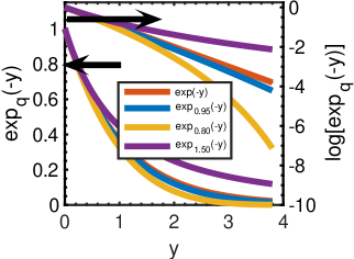
Figure 2: Plots of $\exp(-y)$ and $\exp_{q}(-y)$ (Eq. 17) for different values of the parameter $q$ as a function of $y$

We note some of the properties of the $q$-exponential function ^{46, 39, 40, 15}:

• for $q<1$, $\exp_{q}(y)=0$ for $y<-1/(1-q)$ and $\exp_{q}(y)=\left[1+(1-q)y\right]^{1/(1-q)}$ for $y\geqslant-1/(1-q)$,

• for $q=1$, $\exp_{q}(y)=\exp(y)$ for $\forall y$, and

• for $q>1$, $\exp_{q}(y)=\left[1+(1-q)y\right]^{1/(1-q)}$ for $y<1/(q-1)$.

Fig. 2 shows plots of the deformed $\exp_{q}(-y)$ as a function of $y$ for different values of the parameter $q$ ^{47, 25}. The usual exponential function is also shown for reference. The logarithm of $\exp_{q}(-y)$ provided in the same figure shows linear relationship with $y$ only as $q\to 1$, otherwise, for $q<1$ the curve is convex, and for $q>1$ it is concave ^{48, 35, 36}. In addition to these algebraic properties, the function $\exp_{q}({-y})$ satisfies the anomalous, power-law rate equation $\mathrm{d}y/\mathrm{d}x=-y^{q}$ with $q\neq 1$ ^{49, 28}.

Another important remark on the $q$-exponential and the $q$-Gaussian distributions is that they are the functions associated with some systems showing quasi-stationary states, and are the maximizing distributions for the non-additive Tsallis entropy given by ^{24, 50, 51, 46} :

$$S_{q}=-k\sum_{i}p_{i}^{q}\ln_{q}(p_{i})$$ (19)

where $k$ is a positive constant, $q\neq 1$ (also known as the entropic index), and the quantities $p_{i}=p(E_{i})$ represent the probabilities for the occurrence of the $i^{\text{th}}$ microstate and satisfy $\sum_{i}p_{i}=1$. The function:

$$\ln_{q}(y)=\frac{y^{(1-q)}-1}{1-q}\quad(y>0)$$ (20)

denotes the $q$-logarithm, inverse of the $q$-exponential i.e. $\ln_{q}[\exp_{q}(y)]=\exp_{q}[\ln_{q}(y)]=y$ ⁵¹. In this case, the underlying mathematical mechanism is now the generalized CLT ⁵². It is clear that in the limiting case of $q\to 1$, $\ln_{q}(y)\to\ln(y)$, and one recovers the standard BG entropy $S_{1}=-k_{B}\sum_{i}p_{i}\ln(p_{i})$ where $k=k_{B}$ is the Boltzmann constant ²⁴.

Finally, the generalized $q$-deformed BV model we propose, and incorporating the power-law distribution given by the $q$-exponential function for describing the charge transfer reaction rates dependence on the overpotential and temperature, is given by:

$$i^{*}_{q} =\left[1-(1-q)(-\alpha\eta^{*})\right]^{{1}/{(1-q)}}$$

$$-\left[1-(1-q)(1-\alpha)\eta^{*}\right]^{{1}/{(1-q)}}$$ (21)

$$=\exp_{q}\left[-\alpha\eta^{*}\right]-\exp_{q}\left[(1-\alpha)\eta^{*}\right]$$ (22)

We assumed that the parameter $q$ is the same for both half reactions. Again, recovering the ordinary expression of BV (Eq. 10) is obtained at the limit $q\to 1$. Furthermore, using the the expansion of the $q$-exponential function for sufficiently small values of $y$, i.e. ${\exp_{q}(-y)}=\exp(-y)\left[1+\frac{1}{2}(q-1)y^{2}-\frac{1}{3}(q-1)^{2}y^{3}+\ldots\right]$, one can also recover the usual BV model ³⁹.

2.2 $\kappa$-deformed BV model

In the same way used for the formulation of the $q$-deformed BV model, we propose the following $\kappa$-deformed BV model:

$$i^{*}_{\kappa}=\exp_{\kappa}\left[-\alpha\eta^{*}\right]-\exp_{\kappa}\left[(1-\alpha)\eta^{*}\right]$$ (23)

where the $\kappa$-deformed exponential function of $y$ is given by ²⁶:

$$\exp_{\kappa}(y)\equiv\left(\sqrt{1+\kappa^{2}y^{2}}+\kappa y\right)^{1/\kappa}=\exp\left[\frac{1}{\kappa}\sinh^{-1}(\kappa y)\right]$$ (24)

with $0\leqslant\kappa<1$. The function $\exp_{\kappa}(y)$ emerges from a continuous linear combination of an infinity of standard exponentials as ²⁷:

$$\exp_{\kappa}(-\beta_{0}E)=\int\limits_{0}^{\infty}\frac{1}{\kappa\beta}J_{1/\kappa}\left(\frac{\beta}{\kappa\beta_{0}}\right)\exp({-\beta E})\mathrm{d}\beta$$ (25)

where $J_{\nu}(y)$ is the Bessel function of the first kind. This is equivalent to how the Gamma distribution is the weight function in the generalized Boltzmann factor given by Eq. 12 that led to the $q$-exponential function. Some of the basic properties of $\exp_{\kappa}(y)$ are ²²:

• $\exp_{\kappa\to 0}(y)=\exp(y)$ and $\exp_{\kappa}(y\to 0)=\exp(y)$ ($\exp_{\kappa}(0)=1$);

• $\exp_{\kappa}(y)=\exp_{-\kappa}(y)$;

• for $y\to\infty$, $\exp_{\kappa}(-y)$ is $\sim(2\kappa y)^{-1/\kappa}$ and $\exp_{\kappa}(y)=+\infty$.

Its associated inverse function is the $\kappa$-logarithm:

$$\ln_{\kappa}(y)=\frac{1}{\kappa}\sinh(\kappa\,\ln(y))=\frac{y^{\kappa}-y^{-\kappa}}{2\kappa}$$ (26)

giving $\ln_{\kappa}(\exp_{\kappa}(y))=\exp_{\kappa}(\ln_{\kappa}(y))=y$. Kaniadakis’ entropy associated with the $\kappa$-statistics is obtained by replacing the logarithm in the expression for the standard BG entropy by the $\kappa$-logarithm ^{26, 27, 53, 54}.

Plots of the standard $\exp(-y)$ vs. $\exp_{\kappa}(-y)$ for different values of the parameter $\kappa$ are provided in Fig. 3.

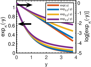
Figure 3: Plots of $\exp(-y)$ and $\exp_{\kappa}(-y)$ (Eq. 24) for different values of $\kappa$ as a function of $y$

3 Results and discussion

In Fig. 4 we show the Tafel plots of electrochemical measurements carried out on a single carbon-coated LiFePO4 particle as-is (i.e. in non-composite structure without interference from the effect of binders and/or other additive conducting materials) from Munakata et al. ¹⁷ and as adjusted by Bai and Bazant ¹ (avoiding concentration polarization effects). Values of current in this single particle technique are usually very small which makes it acceptable to neglect the ohmic $iR$ drop. Low-magnification SEM of the target LiFePO4 particle (see Fig. 2 in ref. ¹⁷) shows that it is spherical in shape, of about 24 $\mu$m in diameter, and consisting of agglomerates of many 100 to 200 nm-sized primary particles with inter-particle porosity and some defects. The specific capacity of the particle was estimated to be 1.5 nA h, and the used discharge current was 750 nA which took just 4 s for full discharge, i.e. 900 C ¹⁷. From the figure, $\ln(i)$ vs. the (normalized) voltage drop is clearly curved and not as expected for traditional Tafel plots. This convex deviation from linearity was attributed by Munakata et al. ¹⁷ to the distributions of electric potential and current density, and also to the distribution of Li^+ concentration within the porous single particle electrode during charging and discharging, which is usually not observed when non-porous flat electrodes are considered. This nonlinear behavior becomes more significant when high rates are applied, which can be further explained as follows. Let us consider the discharge scheme consisting of the steps (i) Li^+ diffusion from the bulk electrolyte to the particle surface, followed by (ii) charge transfer at the particle/electrolyte interface, and then (iii) slow solid-phase diffusion of Li^+ or polaron diffusion from the surface to center of the particle coupled with phase transition from FePO4 to LiFePO4 ¹⁷. Step (iii) is the determining step if there is a large spatial gradient of Li^+ concentration within the particle from surface to center which happens at high discharge current rates, whereas step (ii) may become the controlling step when low rates are applied. In other words, the system can be viewed as a combination of a spectrum of superposed kinetic processes of different origins on the electrode/electrolyte system. If the constituting subsystems are assumed temporarily in local equilibrium and follow Boltzmann exponential profiles with different statistics, it can be well described with the modified BV models as discussed above.

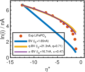
Figure 4: Tafel plots of experimental data by Munakata et al. ^{17, 1} conducted on single carbon-coated LiFePO4 secondary particle (porous with 24 $\mu$m diameter); the potential drop is originally measured with respect to Li/Li^+ but is shown here in dimensionless form as done by Bai and Bazant ¹. We also show data fitting with standard BV model (Eq. 10), the $q$-deformed BV model (Eq. 22) and the $\kappa$-deformed BV model (Eq. 23) with the symmetry factor $\alpha$ set to 0.5

In the same Fig. 4, we show the fitting curves performed with Eq. 22 ($q$-BV model), Eq. 23 ($\kappa$-BV model), and Eq. 10 (standard BV model) with $\alpha=0.5$. We used MATLAB R2019b lsqcurvefit function for nonlinear curve-fitting in least-squares sense with the same fittings constraints and tolerances for all models for fair comparison. When considering the traditional BV model, the data is poorly fitted with a straight line in the semilogarithmic plane of $\ln(i)$ vs. $\eta^{*}$, noting that a better fit can be obtained if a smaller portion of the data is selected closer to $\eta^{*}=0$ (not shown here). The goodness-of-fit using the normalized root mean square error (NRMSE) as the cost function is found to be 0.48, knowing that a value of 1 indicates a perfect fit to the data and $-\infty$ a bad one. The BV model cannot be justified here given the morphological structure of the electrode as described in ref. ¹⁷. From the fitting with the $q$-exponential and $\kappa$-exponential modified BV models, however, it is clear that the curved behavior of the data is closely captured. Convex or concave curvatures can be realized depending on the value of the parameter $q$ for the $q$-deformed model as shown in Fig. 2. Here we found the best fit to be with $q=0.71<1.00$, which phenomenologically indicates the extent of the system’s departure from BG statistics and the associated assumption of thermodynamic equilibrium. For the $\kappa$-deformed BV model we obtained $\kappa=0.47$, which can also be interpreted in a same way, i.e. the extent of the deviation or dispersion of the data from the usual exponential-based BV model that we can retrieve when $\kappa\to 0$. The values of the pre-factor current exchange densities are $i_{0}=21.3$ nA and $i_{0}=16.7$ nA for the $q$- and $\kappa$-deformed models, respectively. The NRMSE fitness values are 0.93 and 0.96, respectively, which are very close to 1. The fittings by both models are very close to each other given the power-law asymptotic behavior of both deformed functions at the relatively large values of the input overpotential. Thus, we are not in the measure to promote or discriminate any of the two without enough information about the local statistics of the electrode.

We note also that the fits are in close agreement with Bai and Bazant’s results ¹ based on MHC theory. The MHC rate is, however, expressed in terms on indefinite integral of the exponential Boltzmann factor (which includes in its argument an extra term representing a reorganization energy) with Fermi-Dirac statistics of electron energies distributed around the electrode potential. This makes the MHC model less attractive from a computational point-of-view. On the other hand, both of the deformed BV models are clearly much simpler and easy to implement with comparable accuracy and fitting capabilities.

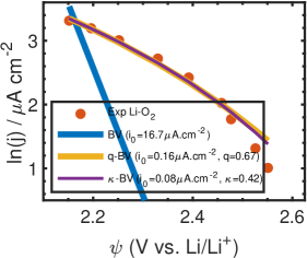
Figure 5: Tafel plots of experimental data by Viswanathan et al. ¹⁸ for the discharge of Li-O2 battery. We also show data fitting with the standard BV model (Eq. 9), $q$-deformed BV model (Eq. 22) and $\kappa$-BV model (Eq. 23) with the symmetry factor $\alpha=0.5$

The curvature of the Tafel plots for other materials and systems may be different, which can still be captured by the free parameters $q$ or $\kappa$ depending on the model as shown in Fig. 5. The figure depicts the experimental Tafel plots of extracted from Viswanathan et al. ¹⁸ for the discharge of Li-air (or Li-O2) battery. The net reaction is $\ce{2Li}+\ce{O2}\rightleftharpoons\ce{Li2O2}$ with the battery discharge described by the forward direction. The nonlinear curve has been attributed to a complex crystal growth and dissolution mechanism of Li2O2 which can occur on different crystal facets or terminations on the electrode, on different sites (terrace, step or kink), and could involve different combinations of nucleation and diffusion ¹⁸ or other mechanisms ¹³. From the figure, it is clear that the standard BV model also fails to adequately fit these types of data, whereas based on different statistics than BG theory, the $q$- and $\kappa$-deformed BV models successfully followed the trend of the curve with ($q=0.67$, $i_{0}=0.16\,\mu\text{A\,cm}^{-2}$) and ($\kappa=0.42$, $i_{0}=0.08\,\mu\text{A\,cm}^{-2}$) respectively. The goodness-of-fit between the models and the experimental data are -0.11, 0.89 and 0.91, respectively.

4 Conclusion

In this contribution, we proposed and verified the application of two deformed versions of the BV model for the analysis of convex semilogarithmic current-overpotential profiles observed with some battery data. The models assume that the nonequilibrium electrode/electrolyte system can be viewed as a multitude of subsystems temporarily in local equilibrium, and thus follow the Boltzmann exponential trend but with different statistics. These fluctuations are taken to be inverse temperature fluctuations that can be correlated for instance to spatial inhomogeneities of the interface geometry, long-range interactions, particle trapping and partial charge transfer, as well as distribution of thermodynamic quantities. Applied to two different examples of battery data ^{17, 18, 1}, both deformed models with only one free parameter each (based on the $q$- or $\kappa$-exponential functions) showed very close agreement with the experiments. The extra degree of freedom in the modified BV models is related to the extent of deviation of the data from BG statistics assumed in classical BV, which itself can be retrieved when $q\to 1$ in Eq. 22 or $\kappa\to 0$ in Eq. 23. The deformed BV models can in principle be applied to other types of usual or unusual reaction data and power-law relaxation behavior found in corrosion reactions, sensors, electrocatalytic processes, solar cells, etc.

References

- Bai and Bazant 2014 Bai, P.; Bazant, M. Z. Charge transfer kinetics at the solid–solid interface in porous electrodes. Nature communications 2014, 5, 1–7
- Dreyer et al. 2016 Dreyer, W.; Guhlke, C.; Müller, R. A new perspective on the electron transfer: recovering the Butler–Volmer equation in non-equilibrium thermodynamics. Physical Chemistry Chemical Physics 2016, 18, 24966–24983
- Marcus 1996 Marcus, R. A. Symmetry or asymmetry of and vs potential curves. J. Chem. Soc., Faraday Trans. 1996, 92
- Chidsey 1991 Chidsey, C. E. D. Free energy and temperature dependence of electron transfer at the metal-electrolyte interface. Science 1991, 251
- Kurchin and Viswanathan 2020 Kurchin, R.; Viswanathan, V. Marcus–Hush–Chidsey kinetics at electrode–electrolyte interfaces. J. Chem. Phys. 2020, 153
- Gutman 2007 Gutman, E. Empiricism or self-consistent theory in chemical kinetics? Journal of alloys and compounds 2007, 434, 779–782
- Yang 2016 Yang, F. Generalized Butler-Volmer relation on a curved electrode surface under the action of stress. SCIENCE CHINA Physics, Mechanics & Astronomy 2016, 59, 1–7
- Fletcher 2009 Fletcher, S. Tafel slopes from first principles. Journal of Solid State Electrochemistry 2009, 13, 537–549
- Vetter 1967 Vetter, K. J. Electrochemical kinetics: theoretical and experimental aspects; Academic Press, 1967
- Pollak and Talkner 2005 Pollak, E.; Talkner, P. Reaction rate theory: What it was, where is it today, and where is it going? Chaos: An Interdisciplinary Journal of Nonlinear Science 2005, 15, 026116
- Li et al. 2018 Li, D.; Lin, C.; Batchelor-McAuley, C.; Chen, L.; Compton, R. G. Tafel analysis in practice. Journal of Electroanalytical Chemistry 2018, 826, 117–124
- Banham et al. 2009 Banham, D. W.; Soderberg, J. N.; Birss, V. I. Pt/carbon catalyst layer microstructural effects on measured and predicted tafel slopes for the oxygen reduction reaction. The Journal of Physical Chemistry C 2009, 113, 10103–10111
- Sankarasubramanian et al. 2017 Sankarasubramanian, S.; Seo, J.; Mizuno, F.; Singh, N.; Prakash, J. Elucidating the oxygen reduction reaction kinetics and the origins of the anomalous Tafel behavior at the lithium–oxygen cell cathode. The Journal of Physical Chemistry C 2017, 121, 4789–4798
- Soderberg et al. 2006 Soderberg, J. N.; Co, A. C.; Sirk, A. H.; Birss, V. I. Impact of porous electrode properties on the electrochemical transfer coefficient. The Journal of Physical Chemistry B 2006, 110, 10401–10410
- Allagui et al. 2021 Allagui, A.; Benaoum, H.; Olendski, O. On the Gouy-Chapman-Stern model of the electrical double-layer structure with a generalized Boltzmann factor. Physica A 2021, 126252
- Boyle et al. 2020 Boyle, D. T.; Kong, X.; Pei, A.; Rudnicki, P. E.; Shi, F.; Huang, W.; Bao, Z.; Qin, J.; Cui, Y. Transient voltammetry with ultramicroelectrodes reveals the electron transfer kinetics of lithium metal anodes. ACS Energy Letters 2020, 5, 701–709
- Munakata et al. 2012 Munakata, H.; Takemura, B.; Saito, T.; Kanamura, K. Evaluation of real performance of LiFePO4 by using single particle technique. Journal of Power Sources 2012, 217, 444–448
- Viswanathan et al. 2013 Viswanathan, V.; Nørskov, J.; Speidel, A.; Scheffler, R.; Gowda, S.; Luntz, A. Li–O2 kinetic overpotentials: Tafel plots from experiment and first-principles theory. The journal of physical chemistry letters 2013, 4, 556–560
- Yin and Du 2014 Yin, C.; Du, J. The collision theory reaction rate coefficient for power-law distributions. Physica A: Statistical Mechanics and its Applications 2014, 407, 119–127
- Claycomb et al. 2004 Claycomb, J.; Nawarathna, D.; Vajrala, V.; Miller Jr, J. Power law behavior in chemical reactions. The Journal of chemical physics 2004, 121, 12428–12430
- Schäfer et al. 2018 Schäfer, B.; Beck, C.; Aihara, K.; Witthaut, D.; Timme, M. Non-Gaussian power grid frequency fluctuations characterized by Lévy-stable laws and superstatistics. Nature Energy 2018, 3, 119–126
- Kaniadakis et al. 2020 Kaniadakis, G.; Baldi, M. M.; Deisboeck, T. S.; Grisolia, G.; Hristopulos, D. T.; Scarfone, A. M.; Sparavigna, A.; Wada, T.; Lucia, U. The -statistics approach to epidemiology. Sci. Rep. 2020, 10, 1–14
- Zhang et al. 2019 Zhang, W.; Wang, X.; Kong, Q.; Ruan, H.; Zuo, X.; Ren, Y.; Cao, Q.; Wang, H.; Zhang, D.; Jiang, J. Power–Law Feature of Structure in Metallic Glasses. The Journal of Physical Chemistry C 2019, 123, 27868–27874
- Tsallis 1988 Tsallis, C. Possible generalization of Boltzmann-Gibbs statistics. J. Stat. Phys. 1988, 52, 479–487
- Tsallis 2019 Tsallis, C. Beyond Boltzmann–Gibbs–Shannon in Physics and Elsewhere. Entropy 2019, 21, 696
- Kaniadakis 2001 Kaniadakis, G. Non-linear kinetics underlying generalized statistics. Physica A: Statistical mechanics and its applications 2001, 296, 405–425
- Kaniadakis 2013 Kaniadakis, G. Theoretical foundations and mathematical formalism of the power-law tailed statistical distributions. Entropy 2013, 15, 3983–4010
- Niven 2006 Niven, R. K. q-Exponential structure of arbitrary-order reaction kinetics. Chemical Engineering Science 2006, 61, 3785–3790
- Bağcı 2007 Bağcı, G. Nonextensive reaction rate. Physica A: Statistical Mechanics and its Applications 2007, 386, 79–84
- Yin and Du 2014 Yin, C.; Du, J. The power-law reaction rate coefficient for an elementary bimolecular reaction. Physica A: Statistical Mechanics and its Applications 2014, 395, 416–424
- Yin et al. 2014 Yin, C.; Guo, R.; Du, J. The rate coefficients of unimolecular reactions in the systems with power-law distributions. Physica A: Statistical Mechanics and its Applications 2014, 408, 85–95
- Cangtao and Du 2014 Cangtao, Y.; Du, J. The power-law reaction rate coefficient for barrierless reactions. Journal of Statistical Mechanics: Theory and Experiment 2014, 2014, P07012
- Aquilanti et al. 2010 Aquilanti, V.; Mundim, K. C.; Elango, M.; Kleijn, S.; Kasai, T. Temperature dependence of chemical and biophysical rate processes: Phenomenological approach to deviations from Arrhenius law. Chemical Physics Letters 2010, 498, 209–213
- Quapp and Zech 2010 Quapp, W.; Zech, A. Transition state theory with Tsallis statistics. Journal of computational chemistry 2010, 31, 573–585
- Silva et al. 2013 Silva, V. H.; Aquilanti, V.; de Oliveira, H. C.; Mundim, K. C. Uniform description of non-Arrhenius temperature dependence of reaction rates, and a heuristic criterion for quantum tunneling vs classical non-extensive distribution. Chemical Physics Letters 2013, 590, 201–207
- Aquilanti et al. 2017 Aquilanti, V.; Coutinho, N. D.; Carvalho-Silva, V. H. Kinetics of low-temperature transitions and a reaction rate theory from non-equilibrium distributions. Philosophical Transactions of the Royal Society A: Mathematical, Physical and Engineering Sciences 2017, 375, 20160201
- Beck 2004 Beck, C. Superstatistics: theory and applications. Continuum Mech. Thermodyn. 2004, 16, 293–304
- Abe et al. 2007 Abe, S.; Beck, C.; Cohen, E. G. Superstatistics, thermodynamics, and fluctuations. Phys. Rev. E 2007, 76, 031102
- Beck and Cohen 2003 Beck, C.; Cohen, E. G. Superstatistics. Physica A 2003, 322, 267–275
- Beck 2006 Beck, C. Stretched exponentials from superstatistics. Physica A: Statistical Mechanics and its Applications 2006, 365, 96–101
- Ourabah 2021 Ourabah, K. Fingerprints of nonequilibrium stationary distributions in dispersion relations. Sci. Rep. 2021, 11, 1–13
- Bondesson 2012 Bondesson, L. Generalized gamma convolutions and related classes of distributions and densities; Springer Science & Business Media, 2012; Vol. 76
- Lienhard and Meyer 1967 Lienhard, J. H.; Meyer, P. L. A physical basis for the generalized gamma distribution. Quarterly of Applied Mathematics 1967, 25, 330–334
- Sebastian 2011 Sebastian, N. A generalized gamma model associated with a Bessel function. Integral transforms and Special functions 2011, 22, 631–645
- Wilk and Włodarczyk 2012 Wilk, G.; Włodarczyk, Z. Consequences of temperature fluctuations in observables measured in high-energy collisions. The European Physical Journal A 2012, 48, 1–13
- Abe and Okamoto 2001 Abe, S.; Okamoto, Y. Nonextensive statistical mechanics and its applications; Springer Science & Business Media, 2001; Vol. 560
- Borges 2004 Borges, E. P. A possible deformed algebra and calculus inspired in nonextensive thermostatistics. Physica A: Statistical Mechanics and its Applications 2004, 340, 95–101
- Truhlar and Kohen 2001 Truhlar, D. G.; Kohen, A. Convex Arrhenius plots and their interpretation. Proceedings of the National Academy of Sciences 2001, 98, 848–851
- Lyra and Tsallis 1998 Lyra, M.; Tsallis, C. Nonextensivity and multifractality in low-dimensional dissipative systems. Phys. Rev. Lett. 1998, 80, 53
- Tsallis 1999 Tsallis, C. Nonextensive statistics: theoretical, experimental and computational evidences and connections. Braz. J. Phys. 1999, 29, 1–35
- Tsallis 2004 Tsallis, C. What should a statistical mechanics satisfy to reflect nature? Physica D 2004, 193, 3–34
- Umarov et al. 2008 Umarov, S.; Tsallis, C.; Steinberg, S. On aq-central limit theorem consistent with nonextensive statistical mechanics. Milan journal of mathematics 2008, 76, 307–328
- Abreu et al. 2018 Abreu, E. M.; Neto, J. A.; Mendes, A. C.; Bonilla, A. Tsallis and Kaniadakis statistics from a point of view of the holographic equipartition law. EPL (Europhysics Letters) 2018, 121, 45002
- Kaniadakis et al. 2017 Kaniadakis, G.; Scarfone, A.; Sparavigna, A.; Wada, T. Composition law of -entropy for statistically independent systems. Physical Review E 2017, 95, 052112