QED with massive photons for precision physics: zero modes and first result for the hadron spectrum

Abstract

The current precision reached by lattice QCD calculations of low-energy hadronic observables, requires not only the introduction of electromagnetic corrections, but also control over all the potential systematic uncertainties introduced by the lattice version of QED. Introducing a massive photon as an infrared regulator in lattice QED, provides a well defined theory, dubbed QED${}_{\textrm{M}}$, amenable to numerical evaluation [1]. The photon mass is removed through extrapolation. In this contribution we scrutinise aspects of QED${}_{\textrm{M}}$ such as the presence and fate of the zero modes contributions and we describe the determination of the photon mass corrections in finite and infinite volume. We demonstrate that the required extrapolations are well controlled using numerical data obtained on two ensembles which only differ in volume.

1 Introduction

Lattice QCD (LQCD) calculations are reaching, for several observables, a control over statistical and systematic effects of the order of the percent and below. An incomplete list includes the recent calculations of radiative leptonic decays of light mesons [2, 3] the baryon spectrum [4], $g_{A}$ [5] and $(g-2)_{\mu}$ [6] . Isospin-breaking (IB) corrections include the difference between the up and down quark masses, $\delta m=m_{u}-m_{d}$, and the electromagnetic interactions between quarks proportional to the electromagnetic coupling $\alpha_{\rm{em}}$. Both IB sources provide, usually, corrections of the order of the percent, as O($\delta m/\Lambda_{\rm{QCD}}$) or O($\alpha_{\rm{em}}$). A sub-percent uncertainty in any LQCD calculation can only be reached if we control IB corrections.

In this contribution we discuss QED corrections. Discretising QED on a finite volume lattice $V=L^{3}\times T$, of sides $L_{\mu}=(L,L,L,T)$, hides subtleties that need to be taken into account for a robust determination of QED corrections to LQCD calculations. QED is usually discretised in a finite volume, see Ref. [7] for a different approach, and the standard choice is to use periodic boundary conditions for the gauge fields. A notable exception is the use of $C^{*}$ boundary conditions proposed in Ref. [8], a formulation called QED${}_{\textrm{C}}$. One of the obstacles that prevent a straightforward implementation of QED on the lattice is the propagation of charged states. It is easy to convince oneself that with periodic boundary conditions charged states in the Hilbert space of the theory are forbidden by Gauss’ law [9, 10]. Given the fact that charged particles are not gauge invariant, one might presume that a local gauge fixing condition would solve the problem, but that is not true. The reason is that, in a finite volume, even after a local gauge fixing procedure, there still exists a gauge transformation, not connected with the identity, that is still a symmetry of the theory: the so-called large gauge transformations (LGT). If we denote the photon and fermion fields respectively with $A_{\mu}(x)$ and $\psi(x),~{}\overline{\psi}(x)$ the LGT read

$$A_{\mu}(x) \rightarrow A_{\mu}^{\prime}(x)=A_{\mu}(x)+2\pi\frac{r_{\mu}}{L_{\mu}}$$

$$\psi(x) \rightarrow \psi^{\prime}(x)=\rm{e}^{i2\pi r_{\mu}\left(\frac{x}{L}\right)_{\mu}}\psi(x)$$

$$\overline{\psi}(x) \rightarrow \overline{\psi}^{\prime}(x)=\overline{\psi}(x)\rm{e}^{-i2\pi r_{\mu}\left(\frac{x}{L}\right)_{\mu}}\,,$$ (1)

where $r_{\mu}\in{\mathbbm{Z}}^{4}$ and $(x/L)_{\mu}=(x_{1}/L,x_{2}/L,x_{3}/L,x_{4}/T)$. LGT are a consequence of the thermal boundary conditions imposed on the fermion fields, and any QED formulation on the lattice has to provide a solution for the breaking of LGT. The solution of this problem relates to the analysis of the zero modes of the photon field.

Most of the solutions proposed, like QED${}_{\textrm{TL}}$ [11] or QED${}_{\textrm{L}}$ [10], remove the zero modes "by hand" introducing potential non-localities in the theory. A discussion on the fate of the zero modes for the most popular QED formulations on the lattice can be found in Ref. [12].

In Ref. [1] we have proposed a discretisation of lattice QED, that introduces a non-zero photon mass, $m_{\gamma}\neq 0$, and labelled as QED${}_{\textrm{M}}$. A first exploratory study of the isospin breaking corrections to $g-2$ computed with QED${}_{\textrm{M}}$ and QED${}_{\textrm{L}}$ has been presented in [13]. In the next section we review some of the properties of QED${}_{\textrm{M}}$  in relation with the fate of the zero modes of the photon.

2 QED${}_{\textrm{M}}$

In Ref. [1] we have introduced a new lattice QED action (QED${}_{\textrm{M}}$)

$$S_{\rm{M}}=a^{4}\sum_{x}\frac{1}{e^{2}}\left[\frac{1}{4}F^{2}_{\mu\nu}+\frac{1}{2\xi}(\partial_{\mu}A_{\mu})^{2}+\frac{1}{2}m_{\gamma}^{2}A^{2}_{\mu}+\overline{\psi}(x)\left(\gamma_{\mu}D_{\mu}+m\right)\psi(x)\right]\,,$$ (2)

where $D_{\mu}$ is the covariant derivative, $F_{\mu\nu}$ is the photon field tensor, and $m$ is the quark mass for a single flavour theory. QED${}_{\textrm{M}}$ features interesting properties: it is renormalisable, it is local, and it is amenable to numerical simulations with a minimal modification with respect to existing codes.

The tree-level photon propagator in a generic R_ξ gauge is given by

$$D_{\mu\nu}(x)=\frac{1}{V}\sum_{q_{\mu}}\rm{e}^{iqx}\frac{1}{q^{2}+m_{\gamma}^{2}}\left[\delta_{\mu\nu}-\frac{q_{\mu}q_{\nu}(1-\xi)}{q^{2}+\xi m_{\gamma}^{2}}\right]\,.$$ (3)

One can immediately see that for $q_{\mu}=0$ the propagator is given by $\delta_{\mu\nu}/(m_{\gamma}^{2}V)$, thus the zero mode contribution diverges in the limit $m_{\gamma}\rightarrow 0$ at fixed finite volume. A standard perturbative expansion in a finite volume would fail in this situation, because it treats all the modes on the same footing. This is another aspect of the fact that, in the limit $m_{\gamma}\rightarrow 0$, the zero modes do not appear in the Gaussian weight of the functional integral. The role of the photon mass term is to provide a dynamical regulator of the zero modes. The solution to this problem is to reorder the perturbative expansion including an arbitrary number of zero-mode propagators. To achieve this goal one treats the zero modes in the functional integral exactly, and the non-zero modes as perturbative corrections. To study the limit of $m_{\gamma}\rightarrow 0$ at fixed volume, it is thus necessary to treat the zero modes exactly.

To simplify the discussion below, and possibly introduce a new computational tool, we decompose the photon field into a zero mode contribution, $B_{\mu}$, and a non-zero mode fluctuation, $q_{\mu}(x)$

$$A_{\mu}(x)=B_{\mu}+q_{\mu}(x)\,.$$ (4)

The zero mode field, $B_{\mu}$, is constant in coordinate space, while the Fourier decomposition of $q_{\mu}(x)$ does not contain the zero momentum term, i.e. $q_{\mu}(x)=\frac{1}{L^{3}T}\sum_{k_{\mu}\neq 0}\rm{e}^{ikx}\widetilde{A}_{\mu}(k)$. If $m_{\gamma}=0$, the zero (constant) modes are unconstrained by the gauge fixing procedure and the theory, as a consequence of the LGT, is still invariant under a shift of the zero mode field [14]

$$B_{\mu}\rightarrow B_{\mu}+2\pi\frac{r_{\mu}}{L_{\mu}}\,.$$ (5)

This redundancy in the functional integral over the zero-mode fields cannot be eliminated by the local gauge fixing procedure, but rather by restricting the integration domain to $0\leq B_{\mu}\leq\frac{2\pi}{L_{\mu}}$. If $m_{\gamma}=0$, the lattice theory in Eq. (2) is invariant under LGT, thus for a generic fermionic correlation function there are $2$ possibilities:

• The fermionic correlation function is invariant under LGT (e.g. neutral particles). In this case we can restrict the integration over the zero modes in the domain $0\leq B_{\mu}\leq\frac{2\pi}{L_{\mu}}$.

• The fermionic correlation function is not invariant under LGT (e.g. charged particles). In this case correlation functions vanish due to the LGT symmetry of the theory. We could insist in defining the correlation functions restricting the integration domains of the zero modes in the domain $0\leq B_{\mu}\leq\frac{2\pi}{L_{\mu}}$. In this way though, we are potentially introducing a non-locality in the correlation function. The fact that the correlation function is not invariant under LGT does not guarantee any more that a LGT will bring the zero mode into the restricted domain.

In the case of QED${}_{\textrm{M}}$ with $m_{\gamma}\neq 0$ LGT are not a symmetry of the theory anymore. This effectively allows us to calculate correlation functions with charged particles, with zero modes that are free to fluctuate because we cannot use LGT anymore to restrict our integration domain.

We conclude that if we integrate the zero modes non-perturbatively in QED${}_{\textrm{M}}$, we should not restrict our integration domain, because the photon mass regulates the fluctuations of the zero modes dynamically. Moreover we expect that correlation functions of charged correlators will vanish as we send the photon mass to zero, $m_{\gamma}\rightarrow 0$, in a finite volume $V$, because in that limit we recover the symmetry under LGT.

The photon mass not only breaks LGT in a local way, but it also provides a mass gap to the theory. The theory now possesses $2$ infrared (IR) cutoffs, $m_{\gamma}$ and $L$, and the order in which these cutoffs are removed is important: first one should perform the infinite volume limit, $L\rightarrow\infty$, at fixed photon mass and then send the photon mass to zero, $m_{\gamma}\rightarrow 0$.

3 Finite volume corrections

To scrutinise whether QED${}_{\textrm{M}}$ is a suitable lattice QED formulation for precision physics, we need to address finite size effects (FSE) specific to this action and understand the role played by the zero modes.

In Sec. 2 we have argued that to study FSE of QED${}_{\textrm{M}}$  when lowering the photon mass, eventually the zero modes have to be treated exactly. We introduce two distinct regimes to analyse finite volume effects. The first regime treats the zero modes of the photon on the same footing as the other modes. In this regime the finite volume corrections are a consequence of the interaction, mediated by photon fields, between copies of matter particles located at distances multiples of $|L_{\mu}|$ between each other. The interaction, mediated by massive photons, produces exponentially suppressed finite volume corrections. This is somehow expected and it is one of the main reasons to introduce QED${}_{\textrm{M}}$.

Finite size corrections are calculated from the self-energy diagrams of matter fields, of mass $M$, with the exchange of a virtual photon. The electromagnetic interaction with coupling $\alpha_{\rm{em}}=e^{2}/4\pi$, shifts the QCD mass of the matter field by an amount $\Delta M=M(\alpha_{\rm{em}})-M(\alpha_{\rm{em}}=0)$ that can be evaluated in a finite volume, $V=L^{3}\times T$, and in infinite volume. The ultraviolet divergences are the same in infinite and finite volume and they cancel out in the subtraction $\delta_{L}M=\Delta M(L)-\Delta M$, where we consider the time extent very large, i.e. $T\gg L$. The calculation of the self-energy in finite and infinite volume gives us the leading contribution proportional to $m_{\gamma}$

$$\delta_{L}M^{LO}=\pi\alpha_{\rm{em}}Q^{2}2m_{\gamma}\mathcal{J}_{1}(m_{\gamma}L)\,,$$ (6)

and the next-to-leading proportional to $m_{\gamma}^{2}/M$

$$\delta_{L}M^{NLO}=\pi\alpha_{\rm{em}}Q^{2}m_{\gamma}\frac{m_{\gamma}}{M}\left[2\mathcal{J}_{1/2}(m_{\gamma}L)+\mathcal{J}_{3/2}(m_{\gamma}L)\right]\,,$$ (7)

where $Q$ is the charge of the particle in units of $e$, and $\mathcal{J}_{n}(z)$ are linear combinations of modified Bessel functions

$$\mathcal{J}_{n}(z)=\frac{1}{2^{n+{1\over 2}}\pi^{{3\over 2}}\Gamma(n)}\sum_{\mathbf{\nu}}\frac{K_{{3\over 2}-n}(z|\mathbf{\nu}|)}{(z|\mathbf{\nu}|)^{{3\over 2}-n}}\,.$$ (8)

In comparison with Ref. [1], this expression does not include the contributions from the zero modes, which we discuss separately in the next section.

3.1 Zero modes

For the calculation of the zero-mode contributions to the finite size effects we introduce a new computational tool and regime. We call the region in parameter space where the zero modes of the photons cannot be treated perturbatively the $\epsilon_{\gamma}$ regime. In this regime we treat the zero modes of the photon field exactly in the functional integral and we expand the non-zero mode contributions perturbatively. In Eq. (4) we have decomposed the photon field in a constant field, $B_{\mu}$, and the fluctuations, $q_{\mu}(x)$, that do not contain zero modes. If we rewrite the QED${}_{\textrm{M}}$ action in Eq. (2) and, as leading contribution, we set $q_{\mu}(x)=0$ we obtain

$$S_{\rm{M}}=\frac{1}{2}\frac{m_{\gamma}^{2}V}{e^{2}}B^{2}+a^{4}\sum_{x}\overline{\psi}\left\{\gamma_{\mu}\left[\partial_{\mu}+iB_{\mu}\right]+M\right\}\psi\,,$$ (9)

where we have removed all terms containing the non-zero modes fluctuations.

We notice that the zero modes contribute in two ways: a shift in the momentum of the matter propagator from the matter part of the action, and a Gaussian measure factor from the gauge part of the action. We start by calculating the partition function

$${\mathcal{Z}}_{0}=\int{\mathcal{D}}[B_{\mu},\psi,\overline{\psi}]\rm{e}^{-\frac{1}{2}\frac{m_{\gamma}^{2}V}{e^{2}}B^{2}}\rm{e}^{-\int d^{4}x\overline{\psi}\left\{\gamma_{\mu}\left[\partial_{\mu}+iB_{\mu}\right]+M\right\}\psi}\,,$$ (10)

where we have assumed that $q_{\mu}(x)=0$ and we consider the continuum formulation of the theory. For the time being we neglect the functional integral on the fermions consistently with the fact that in our numerical simulations we do not include QED fermion loops. Neglecting the QED quark determinant we obtain

$${\mathcal{Z}}_{0}=\left(\frac{2e^{2}\pi}{m_{\gamma}^{2}V}\right)^{2}\,.$$ (11)

The next step is to calculate the two-point functions. Projecting to zero spatial momentum

$$C(x_{4};{\bf p}=0)=\int d^{3}x~{}\left\langle\psi(x)\overline{\psi}(0)\right\rangle=\frac{1}{{\mathcal{Z}}_{0}}\int{\mathcal{D}}[B_{\mu}]\rm{e}^{-\frac{1}{2}\frac{m_{\gamma}^{2}V}{e^{2}}B^{2}}\frac{1}{T}\sum_{k_{4}}\rm{e}^{ik_{4}x_{4}}\frac{-i\gamma_{4}k_{4}-i\not{B}+M}{\left(k_{4}+B_{4}\right)^{2}+\omega_{B}^{2}}\,,$$ (12)

where the location of the pole is shifted because of the presence of the zero modes

$$\omega_{B}^{2}=M^{2}+|{\bf B}|^{2}\,.$$ (13)

For simplicity, we neglect the Dirac structure in the numerator, and consider only the propagator of a scalar particle. The integrand

$${\mathcal{C}}(x_{4};{\bf p}=0;B)\rightarrow\frac{1}{T}\sum_{k_{4}}\rm{e}^{ik_{4}x_{4}}\frac{1}{\left(k_{4}+B_{4}\right)^{2}+\omega_{B}^{2}}\,,$$ (14)

can be calculated using a Schwinger parametrisation. The sum over $k_{4}$ can be done exactly and for large $T$ the leading term is given by the infinite volume time-momentum representation

$${\mathcal{C}}(x_{4};{\bf p}=0;B)\simeq\rm{e}^{-iB_{4}x_{4}}\frac{\rm{e}^{-\omega_{B}x_{4}}}{2\omega_{B}}\,.$$ (15)

We conclude that the leading finite size corrections correspond to the integration over the zero modes of the "infinite volume" propagator projected to zero momentum. We can now finalise the calculation of

$$C(x_{4};{\bf p}=0)=\frac{1}{{\mathcal{Z}}_{0}}\int{\mathcal{D}}[B_{\mu}]\rm{e}^{-\frac{1}{2}\frac{m_{\gamma}^{2}V}{e^{2}}B^{2}}\rm{e}^{-iB_{4}x_{4}}\frac{\rm{e}^{-\omega_{B}x_{4}}}{2\omega_{B}}\,.$$ (16)

After few lines of algebra we obtain

$$C(x_{4};{\bf p}=0)=\rm{e}^{-\zeta x_{4}^{2}}\rm{e}^{-Mx_{4}}{\mathcal{I}}(x_{4},M,m_{\gamma},V)\,,$$ (17)

where we defined the zero mode parameter $\zeta$

$$\zeta=\frac{e^{2}}{2m_{\gamma}^{2}V},$$ (18)

and the integral ${\mathcal{I}}$ is given by

$${\mathcal{I}}(x_{4},M,m_{\gamma},V)=\frac{1}{\overline{\mathcal{Z}}_{0}}\int d^{3}B~{}\frac{\rm{e}^{-\frac{1}{2}\frac{m_{\gamma}^{2}V}{e^{2}}|{\bf B}|^{2}}\rm{e}^{-(\omega_{B}-M)x_{4}}}{2\omega_{B}}\,,$$ (19)

where

$$\overline{\mathcal{Z}}_{0}=\int d^{3}B~{}\rm{e}^{-\frac{1}{2}\frac{m_{\gamma}^{2}V}{e^{2}}|{\bf B}|^{2}}\,.$$ (20)

We obtain the result of Ref. [1] showing that the leading exponential behaviour of the correlation function is modified by the zero modes, inducing a linear rise in $x_{4}$ in the effective mass proportional to $\zeta$. This correction is a finite size effect and it does not imply the lack of a transfer matrix in the theory. The lattice action is ultra-local and it would not be difficult to construct an explicit expression for the transfer matrix. There are other examples, like the $\epsilon$ regime of chiral perturbation theory, where the Euclidean time dependence of correlation functions is not a sum of exponential functions and still the theory possesses a transfer matrix [15].

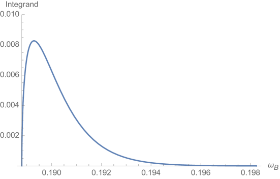
Figure 1: Integrand, Eq. (22), for $am_{\gamma}=0.0236$, $m_{\gamma}/M=1/8$ and $(L/a)^{3}\times T/a=24^{3}\times 64$.

We now want to scrutinise the contribution of the spatial zero modes in Eq. (19). The integral ${\mathcal{I}}$ can be simplified using polar coordinates

$${\mathcal{I}}(x_{4},M,m_{\gamma},V)=2\pi\left(\frac{m_{\gamma}^{2}V}{2e^{2}\pi}\right)^{3/2}\rm{e}^{Mx_{4}}\rm{e}^{\frac{m_{\gamma}^{2}M^{2}V}{2e^{2}}}\int_{M}^{\infty}d\omega_{B}~{}\sqrt{\omega_{B}^{2}-M^{2}}\rm{e}^{-\frac{1}{2}\frac{m_{\gamma}^{2}V\omega_{B}^{2}}{e^{2}}}\rm{e}^{-\omega_{B}x_{4}}\,.$$ (21)

In Fig. 1 we plot the integrand

$$\sqrt{\omega_{B}^{2}-M^{2}}\rm{e}^{-\frac{1}{2}\frac{m_{\gamma}^{2}V(\omega_{B}^{2}-M^{2})}{e^{2}}}\rm{e}^{-(\omega_{B}-M)x_{4}}\,,$$ (22)

as a function of $\omega_{B}$ for the most extreme value of the simulation parameters described below, i.e. $m_{\gamma}/M=1/8$ and $V/a^{4}=24^{3}\times 64$. The peak is slightly shifted from $M$ and when increasing the volume both the location of the peak and its width shrink to zero. The integrand itself vanishes when $V\rightarrow\infty$. The analytical estimate of the integral can be done with a saddle point approximation. To avoid the zero in the leading term, we include the sub-leading terms in $1/V$ in the approximation. We rewrite

$${\mathcal{I}}(x_{4},M,m_{\gamma},V)=2\pi\left(\frac{m_{\gamma}^{2}V}{2e^{2}\pi}\right)^{3/2}\int_{M}^{\infty}d\omega_{B}~{}\rm{e}^{V\left[-\frac{1}{2}\frac{m_{\gamma}^{2}(\omega_{B}^{2}-M^{2})}{g^{2}}-\frac{(\omega_{B}-M)}{V}x_{4}+\frac{1}{2V}\log\left(\omega_{B}^{2}-M^{2})\right)\right]}\,.$$ (23)

In the limit $V\rightarrow\infty$ we can now use the saddle point approximation including the second and third exponentials that are sub-leading. Using the usual machinery and evaluating the second derivative of the exponent we find, up to higher order corrections in $1/V$

$${\mathcal{I}}(x_{4},M,m_{\gamma},V)=\left(\frac{8\pi\alpha_{\rm{em}}m_{\gamma}^{2}V}{\rm{e}M^{2}}\right)^{1/2}\rm{e}^{-\frac{\zeta}{M}x_{4}}\,,$$ (24)

where the saddle point is given by

$$\overline{\omega}_{B}=M\left(1+\frac{\zeta}{M^{2}}\right)\,.$$ (25)

To avoid confusion we denote the electric charge in terms of $\alpha_{\rm{em}}=e^{2}/4\pi$, while the $\rm{e}$ in Eq. (24) and in the following denotes Euler’s number. The correlation function in Eq. (17) now reads

$$C(x_{4};{\bf p}=0)=\left(\frac{8\pi\alpha_{\rm{em}}m_{\gamma}^{2}V}{\rm{e}M^{2}}\right)^{1/2}\rm{e}^{-\zeta x_{4}^{2}}\rm{e}^{-M(1+\frac{\zeta}{M^{2}})x_{4}}\,,$$ (26)

thus the mass extracted from an effective mass analysis will contain two types of finite size effects

$$m_{\textrm{eff}}=-\frac{d}{dx_{4}}\log C(x_{4};{\bf p}=0)=2\zeta x_{4}+M\left(1+\frac{\zeta}{M^{2}}\right)\,,$$ (27)

coming from the temporal zero modes, modifying the Euclidean time dependence of the correlation function, and from spatial zero modes shifting the mass. We notice, that as predicted in Sec. 2 the correlation function vanishes if we send the photon mass to zero at fixed finite volume.

For our ensemble at $M=M_{\pi}\simeq 310$ MeV, $(L/a)^{3}\times T/a=24^{3}\times 64$ and $m_{\gamma}/M_{\pi}=1/8,1/4$, which are the worse possible cases together with the lightest photon mass $m_{\gamma}/M_{\pi}=1/8$ at the largest volume $(L/a)^{3}\times T/a=48^{3}\times 64$, we obtain finite size effects relative to the matter field mass of $0.024\%$, $0.006\%$ and $0.003\%$, respectively. If the QED corrections are at the percent level, these finite size corrections contribute a $2.4\%$ correction in the worse case. As discussed in Sec. 5.2, the smallest photon mass will not be included in the final analysis. We conclude that once the temporal zero modes corrections are exactly subtracted from the effective mass analysis the remaining effects stemming from the spatial zero modes can be safely neglected, possibly with the exception of the case $(L/a)^{3}\times T/a=24^{3}\times 64$ and $m_{\gamma}/M_{\pi}=1/8$.

3.2 Dispersion relation

A final remark concerns the contribution of the zero modes to the energy spectrum at non-zero spatial momentum. In Ref. [12] it was pointed out that finite volume corrections for QED${}_{\textrm{M}}$ can cause a suppression of the dependence on the momentum in the effective energy.

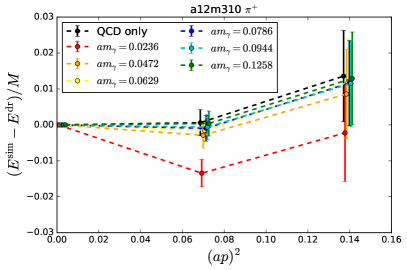
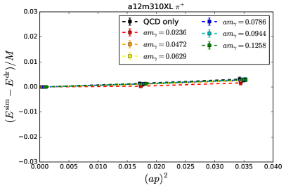
Figure 2: Relative discrepancy between the expected lattice dispersion relation and the computed energy for the charged pion as a function of momentum for the various simulated photon masses on the a12m310 (left) and the a12m310XL (right) ensembles. To ease the comparison we use the same scale in the y-axis.

In other words if the photon mass is too small at fixed finite volume, the dispersion relation can be violated. We determined the energy of the charged pion as a function of the momentum of the pion, $E^{\rm{sim}}(p^{2})$ for several photon masses (see Sec. 5 for details of the numerical analysis). We then compared the results from the simulations to the expected lattice dispersion relation

$$\sinh\left(\frac{aE^{\textrm{dr}}}{2}\right)=\sinh\left(\frac{aM}{2}\right)+\sum_{i=1}^{3}\sin^{2}\left(\frac{ap_{i}}{2}\right)\,.$$ (28)

In Fig. 2 we show $\frac{E^{\rm{sim}}(p^{2})-E^{\textrm{dr}}}{M}$ as a function of $p^{2}$. Different colours show results with different photon masses; the left plot corresponds to the small volume, while the right plot the larger volume. We observe that, beside the smallest photon mass in the small volume, all the energies computed satisfy the expected dispersion relation. As a check of the procedure we also show the same quantity for pure QCD, obtaining the same type of agreement.

We conclude that the dispersion relation is a useful quantity to monitor in order to check the contribution of the photon zero modes. In our numerical studies only the smallest photon mass on the ensemble with the smaller volume, corresponding to $m_{\gamma}L=0.53$, deviates from the expected form of the dispersion relation.

4 Computational Set-Up

Having laid the analytic ground work to assess the finite size effects we now turn our attention to numerical tests. The main goal of this section is to establish a region in parameter space, where the required limits i.e. the extrapolations to the infinite volume and subsequently to vanishing photon mass, are well controlled. To this end, we compute the mass splittings due to QED isospin breaking effects for two ensembles with identical parameters except the spatial volume. On these ensembles we simulate a range of six different photon masses given by $m_{\gamma}=\{1/8,1/4,1/3,5/12,1/2,2/3\}\times M_{\pi}$. If the finite size effects are indeed well described, the simulations performed on the different volumes need to produce compatible results once the infinite volume extrapolation has been performed.

Numerically, we utilise the mixed-action set-up established by the CalLat collaboration [16] using gauge field configurations with $N_{f}=2+1+1$ dynamical highly improved (rooted) staggered quarks (HISQ) [17] in the sea which are gradient flowed prior to inverting Möbius domain wall fermions in the valence sector. We use the a12m310 (from MILC [18]) and a12m310XL (from CalLat [19]) ensembles. These ensembles have a lattice spacing $a\approx 0.12$ fm, identical sea quark masses resulting in a pion mass of approximately $310\,\mathrm{MeV}$ and 4-volumes of $L^{3}\times T/a^{4}=24^{3}\times 64$ and $48^{3}\times 64$. Our computations are performed in the electro-quenched approximation using stochastic $U(1)$ background gauge fields which are fixed to Landau gauge.

5 Data Analysis

We generate two-point correlation functions $C_{\mathbb{P}^{Q}}^{SY}(t;m_{\gamma})$ inducing the quantum numbers of a state $\mathbb{P}$ with charge $Q$. Here the “S” indicates that the source of the propagators is always Gaussian smeared, whilst the sink can be point-like or smeared ($Y\in\{P,S\}$). Omitting the backwards travelling contribution to the correlation functions, we write the isospin symmetric correlation function as

$$C^{SY}_{\bar{\mathbb{P}}}(t)=\sum_{i}\frac{\bar{Z}_{i}^{S}\bar{Z}_{i}^{Y}}{2\bar{M}_{i}}e^{-\bar{M}_{i}t}.$$ (29)

We express the masses and amplitudes in the presence of QED as the splittings $\delta Z_{i}$ and $\delta M_{i}$ to the isospin symmetric quantities, i.e.

$$C^{SY}_{\mathbb{P}^{Q}}(t;m_{\gamma})=\sum_{i}\frac{\left(\bar{Z}_{i}^{S}+\delta Z_{i}^{S}(m_{\gamma})\right)\left(\bar{Z}_{i}^{Y}+\delta Z_{i}^{Y}(m_{\gamma})\right)}{2\left(\bar{M}_{i}+\delta M_{i}(m_{\gamma})\right)}e^{-\left(\bar{M}_{i}+\delta M_{i}(m_{\gamma})\right)t-\zeta(m_{\gamma})t^{2}},$$ (30)

where $\zeta(m_{\gamma})$ is the contribution from the zero-mode as defined in (18). For light mesonic states we have to consider the backwards travelling contributions given by a second term with $t\to(T-t)$. Note that this can be simplified using

$$e^{-mt}+e^{-m(T-t)} =2e^{-\frac{mT}{2}}\mathrm{cosh}\left[m\left(t-\frac{T}{2}\right)\right],$$ (31)

$$e^{-mt-\zeta t^{2}}+e^{-m(T-t)-\zeta(T-t)^{2}} =2e^{-\frac{(m+\zeta T)T}{2}}\mathrm{cosh}\left[\left(m+\zeta T\right)\left(t-\frac{T}{2}\right)\right]e^{-\zeta\left(t^{2}-tT\right)}.$$

Even though we have a large data set for the meson and baryon octets and the baryon decouplet, here we are mostly interested in the sensitivity to the infrared regularisation so in the following we will mostly focus on the lightest states $\mathbb{P}^{Q}=\pi^{\pm}$, $\pi^{0}$, $K^{\pm}$ and $K^{0}$.

5.1 Correlator analysis and zero mode

We note that the term involving the zero mode $\zeta$ is analytically completely determined. Prior to any correlation function analysis, we remove this by hand by multiplying the relevant correlation functions by $e^{\zeta t^{2}}$ (if the backwards propagating part is negligible) and $e^{\zeta(t^{2}-tT)}$ (otherwise). In the latter case, one can then fit the correlation function to the typical functional form and obtain $m+\zeta T$ (see (31)). Clearly $\zeta T$ can then be subtracted analytically.

Figure 3: Effective mass splittings for charged pions. The correlated difference between effective masses in the presence of QED and the QCD effective mass is shown. The zero mode leads to a linear rise in the effective mass (faint symbols), which can be removed analytically (filled symbols).

Figure 3 shows the effective mass splitting for the charged pion as a function of photon mass (different colours) and spatial volume (left vs right panel). This is obtained by taking the correlated difference of the effective masses from the correlation functions with QED to those using the QCD only correlation function. The faint symbols show a linear rise stemming from the zero mode. The closed symbols demonstrate that once the zero mode is removed, one obtains very stable plateaus in the effective mass splitting. When comparing the effective mass splittings between the a12m310 (left) and the a12m310XL (right) ensembles, we notice a significant dependence on the volume. We re-iterate that these two simulations only differ in the doubled spatial extents of the a12m310XL ensemble.

In order to extract mass splittings it is beneficial to consider the following ratios of correlation functions

$$R^{SY}_{\mathbb{P}^{Q}}(t;m_{\gamma}) =\frac{e^{-\zeta\left(t^{2}+\frac{T^{2}}{2}-tT\right)}C^{SY}_{\mathbb{P}^{Q}}(t;m_{\gamma})}{C^{SY}_{\bar{\mathbb{P}}}(t)}$$ (32)

$$=\frac{\sum_{i}\left(\bar{Z}_{i}^{S}+\delta Z_{i}^{S}\right)\left(\bar{Z}_{i}^{Y}+\delta Z_{i}^{Y}\right)\mathrm{cosh}\left[\left(\bar{M}_{i}+\delta M_{i}+\zeta T\right)\left(t-\frac{T}{2}\right)\right]e^{-(\bar{M}_{i}+\delta M_{i})T/2}/\left(\bar{M}_{i}+\delta M_{i}\right)}{\sum_{j}\bar{Z}_{j}^{S}\bar{Z}_{j}^{Y}\mathrm{cosh}\left[\bar{M}_{j}\left(t-\frac{T}{2}\right)\right]e^{-\bar{M}_{j}T/2}/\bar{M}_{j}}$$

$$\approx\left(1+\frac{\delta Z^{S}_{0}}{Z^{S}_{0}}+\frac{\delta Z^{Y}_{0}}{Z^{Y}_{0}}-\frac{\delta M_{0}}{\bar{M_{0}}}\right)e^{-\delta M_{0}t}+\mathcal{O}(e^{-\Delta\bar{M}_{1}t},e^{-(\Delta\bar{M}_{1}+\delta M_{0})t},e^{-(\Delta\bar{M}_{1}+\delta M_{1})t},\delta^{2}),$$

where $\delta X_{i}$ refers to the QED-induced splittings of the i^th excited state of the observable $X$ and $\Delta X_{i}$ to splitting between the i^th excited state and the ground state. In addition to being very sensitive to the mass splitting, the high degree of correlation between the two correlation functions that enter the ratio results in very favourable statistical properties. This leads to the correlation matrix that enters the fit to be close to block diagonal. An example of such a correlation matrix is shown for the charged pion correlation functions on the a12m310 ensemble in Figure 4.

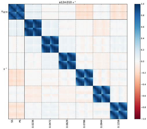
Figure 4: Correlation matrix entering the correlated fit to extract the QCD parameters and the QED induced splittings.

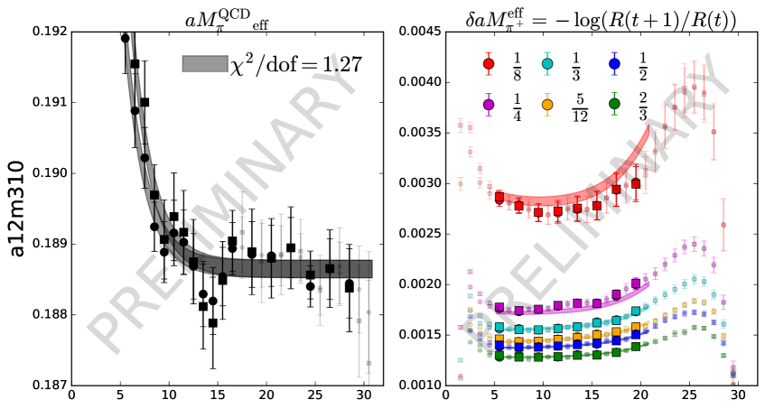
Figure 5: Fit results superimposed to the effective mass (left) and mass splittings (right) for the charged pion.

In order to obtain all required matrix elements, masses and their splittings, we perform a simultaneous correlated fit to the isospin symmetric correlation functions $C^{SY}_{\mathbb{P}^{Q}}(t;m_{\gamma})$ and the ratios $R^{SY}_{\mathbb{P}^{Q}}(t;m_{\gamma})$ including the ground state and first excited state throughout. An example projection to the effective masses of such a fit is shown in Figure 5. All 14 correlation functions (6 different photon masses and the QCD only correlation function, each for two different smearing choices) are well described by a single correlated fit. We assess the stability of this fit by systematically varying the fit ranges as well as by consecutively removing the data corresponding to the lightest photon masses from the fit. We show the stability of the mass splittings to the isospin symmetric pion mass in Figure 6. We observe that removing the lightest photon mass(es) from the fit does not change the remaining fit results, indicating stability.

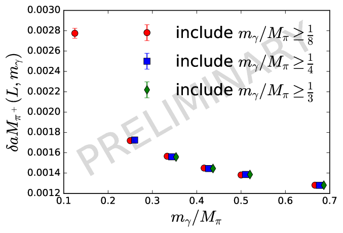
Figure 6: Extracted QED-induced mass splittings in the pion for a number of cuts to the smallest included photon mass on the a12m310 ensemble. The data points are slightly staggered along the horizontal axis for better visibility.

5.2 Infinite volume limit

In order to make precise predictions with fully controlled systematic uncertainties, one has to carefully investigate all required limits. Before taking the vanishing photon mass limit, we need to correct the data for the finite size effects and extrapolate to infinite volume. As discussed above, given the infrared nature of the photon mass, the finite size effects are of crucial importance. We generated data on two ensembles with identical parameters other than their spatial volume, precisely for this reason, i.e. this study is designed to test how accurately these corrections describe our data. We test this by removing the leading and next to leading order finite size corrections from the data by applying the corrections detailed in (6) and (7). However, care must be taken since the zero-mode contributions are assumed to be present in the development of the formalism for the finite volume corrections, but the zero mode has already been removed by hand. We follow the prescription described in Ref. [1] and add and subtract the zero mode in order to complete the sum in (6). This results in an additional finite volume correction $\delta_{L}^{\mathrm{zm}}$ defined by

$$\delta_{L}^{\mathrm{zm}}=-2\pi\alpha Q^{2}m_{\gamma}\frac{1}{(m_{\gamma}L)^{3}}.$$ (33)

We stress that this is work in progress and likely only an effective approximation for sufficiently large temporal extents. One concern is that the zero mode contribution (33) does not vanish as $T\to\infty$, even though the quantity $\zeta$ defined in (18) does. Given the identical temporal extent of the two ensembles presented here, this contribution is expected to be the same for both ensembles, thereby allowing us to meaningfully compare the finite volume effects using the data at hand. We expect to provide further analytical work and numerical evidence, taking the finite four-volume into account in the near future.

Figure 7 shows the various contributions that are subtracted from the data to recover a good approximation for the infinite volume limit. In particular $\delta_{L}^{\mathrm{LO}}$ (dotted lines), $\delta_{L}^{\mathrm{zm}}$ (dashed lines) and $\delta_{L}^{\mathrm{NLO}}$ (dash-dotted lines) are shown as well as their total (solid lines). The ensemble with the smaller volume (a12m310) is shown in red, whilst the larger volume result (a12m310XL) is shown in blue. These contributions are evaluated for a pion mass of $310\,\mathrm{MeV}$ and a proton mass of $1000\,\mathrm{MeV}$. As expected the individual finite size effects are larger for the smaller volume. Also in agreement with expectation, the finite size effects are more pronounced for the pion than for a proton.

We observe that $\delta_{L}^{\mathrm{zm}}$ and $\delta_{L}^{\mathrm{LO}}$ are similar in magnitude but have an opposite sign leading to large cancellations, causing the sum of the contributions to change sign for very small photon masses. Clearly the finite volume formulae are insufficient to accurately describe the corrections for such very small photon masses. For this reason we remove the smallest photon masses on the smaller volume in all cases and carefully study the effect of removing further photon masses close to this regime.

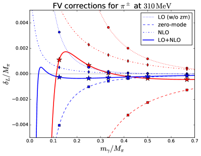
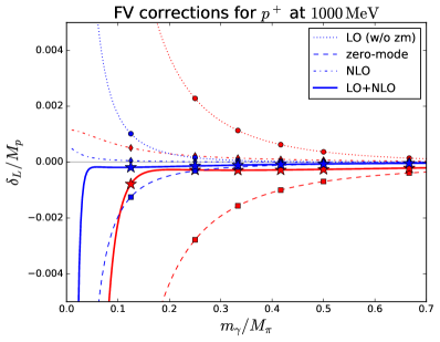
Figure 7: Individual contributions to the finite volume corrections as a function of $m_{\gamma}/M_{\pi}$. The red (blue) data represent the lattice parameters of the a12m310 (a12m310XL) ensemble. The left panel shows the relative size for a pion mass of $310\,\mathrm{MeV}$, the right hand panel for a proton of $1000\,\mathrm{MeV}$. The symbols correspond to the simulated data points on these ensembles.

Figure 8 shows the mass splittings of the charged pion (left) and the charged kaon (right) for the two simulated ensembles as a function of the photon mass. The simulated data points prior to any finite size corrections are shown as the open symbols, the mass splittings after the finite size corrections have been applied are shown as the closed symbols. After the leading order and next-to-leading order finite size effects have been removed, the data show good agreement between the two ensembles, particularly for the larger photon masses.

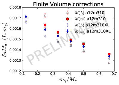
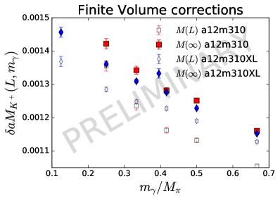
Figure 8: The effect of the finite volume corrections in the QED-induced mass splitting of the charged pion (left) and the charged kaon (right). Open symbols show the mass splittings extracted from the simulation, closed symbols the mass splittings after the finite volume corrections have been applied.

5.3 Vanishing photon mass limit

Finally it remains to take the $m_{\gamma}\to 0$ limit to remove the second infrared regulator. This is guided by an effective field theory approach [1]. The limit $m_{\gamma}\to 0$ is parameterised as

$$M(0)=M(m_{\gamma})-\Delta_{\gamma}M^{\mathrm{LO}}-\Delta_{\gamma}M^{\mathrm{NLO}}+\mathcal{O}\left(\frac{m_{\gamma}^{3}}{M^{2}}\right),$$ (34)

where the leading order and next-to-leading order corrections are given by

$$\Delta_{\gamma}M^{\mathrm{LO}}=-\frac{\alpha}{2}Q^{2}m_{\gamma}$$ (35)

and

$$\Delta_{\gamma}M^{\mathrm{NLO}}=\left(C\alpha-\frac{\alpha}{4\pi}Q^{2}\right)\frac{m_{\gamma}^{2}}{M}.$$ (36)

Here $M(0)$ is the result for the mass (or mass splitting) at zero photon mass, $Q$ is the charge of the hadron and $C$ is a low energy constant that can be determined through a fit to the data. This correction arises from “hard-photon” corrections between the quarks comprising the hadron.

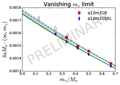
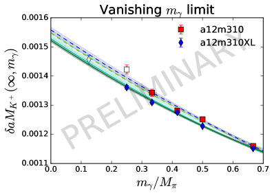
Figure 9: Examples of the vanishing photon mass extrapolation of the data obtained by the finite volume corrections for the case of the mass splitting of the charged pion (left) and the charged kaon (right).

We perform the extrapolation as a fit to the different photon mass data points. Figure 9 shows the result for the mass splitting of the charged pion (left) and the charged kaon (right) on the two ensembles. The data points in these plots are the results from applying the finite size effects in the previous section. The closed symbols correspond to data points entering the chosen fit, the open symbols are excluded from the chosen fit. Additional coloured lines correspond to alternative fits where consecutively more of the lighter photon masses are removed, which all provide stable results.

Due to the size of the finite size effects we exclude the lightest photon mass on the larger ensemble (red squares, a12m310XL) and the lightest two photon masses on the smaller ensemble (blue diamonds, a12m310). We obtain statistically compatible low energy constants $C$ from the two fits. This preliminary analysis is based solely on statistical uncertainties, i.e. we have not yet included any systematic error budget for choices made in the correlation function fits or included estimates of higher order finite volume corrections. The agreement at vanishing photon mass is very encouraging and indicates that all the required limits are under control.

6 Summary and Outlook

We have presented numerical results using massive QED to compute QED effects in precision lattice QCD simulations. We find a good statistical signal, allowing us to determine QED induced splittings of masses and matrix elements though a suitably chosen combined fit to correlation functions and ratios of correlation functions. We explicitly treat the zero mode contribution and find good control over the two consecutive limits of $L\to\infty$ and $m_{\gamma}\to 0$ which are both guided by effective field theories. We produce numerically compatible results on two ensembles which differ by a factor of two in the spatial extents, lending confidence to the chosen approach. We thereby demonstrated that the absence of power-like finite volume effects in the approach of QED${}_{\textrm{M}}$ enables the use of existing gauge field configurations with $M_{\pi}L\gtrsim 4$ for precision predictions of isospin breaking effects and thereby provide a cost efficient framework.

The results presented here are part of a larger body of work including strong isospin breaking contributions, the meson and octet spectrum, QED effects on the $\Omega^{-}$ baryon mass which is frequently used to set the lattice scale (e.g. [6, 19]), QED corrections to $g_{A}$, investigations of the $\Lambda^{0}-\Sigma^{0}$ mixing and QED corrections required for CKM physics. We are also numerically testing the scheme proposed in [20] to separate strong and weak isospin breaking effects. Data has been produced on further ensembles allowing to take a continuum limit with three lattice spacings at a pion mass of $310\,\mathrm{MeV}$ and data production for lighter pion masses is ongoing.

References

- [1] Michael G. Endres, Andrea Shindler, Brian C. Tiburzi, and Andre Walker-Loud. Massive photons: an infrared regularization scheme for lattice QCD+QED. Phys. Rev. Lett., 117(7):072002, 2016.
- [2] D. Giusti, V. Lubicz, G. Martinelli, C. T. Sachrajda, F. Sanfilippo, S. Simula, N. Tantalo, and C. Tarantino. First lattice calculation of the QED corrections to leptonic decay rates. Phys. Rev. Lett., 120(7):072001, 2018.
- [3] R. Frezzotti, M. Garofalo, V. Lubicz, G. Martinelli, C. T. Sachrajda, F. Sanfilippo, S. Simula, and N. Tantalo. Comparison of lattice QCD+QED predictions for radiative leptonic decays of light mesons with experimental data. Phys. Rev. D, 103(5):053005, 2021.
- [4] Sz. Borsanyi et al. Ab initio calculation of the neutron-proton mass difference. Science, 347:1452–1455, 2015.
- [5] C. C. Chang et al. A per-cent-level determination of the nucleon axial coupling from quantum chromodynamics. Nature, 558(7708):91–94, 2018.
- [6] Sz. Borsanyi et al. Leading hadronic contribution to the muon magnetic moment from lattice QCD. Nature, 593(7857):51–55, 2021.
- [7] Thomas Blum, Norman Christ, Masashi Hayakawa, Taku Izubuchi, Luchang Jin, Chulwoo Jung, and Christoph Lehner. Using infinite volume, continuum QED and lattice QCD for the hadronic light-by-light contribution to the muon anomalous magnetic moment. Phys. Rev. D, 96(3):034515, 2017.
- [8] Biagio Lucini, Agostino Patella, Alberto Ramos, and Nazario Tantalo. Charged hadrons in local finite-volume QED+QCD with C∗ boundary conditions. JHEP, 02:076, 2016.
- [9] Michael Creutz. Quantum Electrodynamics in the Temporal Gauge. Annals Phys., 117:471, 1979.
- [10] Masashi Hayakawa and Shunpei Uno. QED in finite volume and finite size scaling effect on electromagnetic properties of hadrons. Prog. Theor. Phys., 120:413–441, 2008.
- [11] A. Duncan, E. Eichten, and H. Thacker. Electromagnetic splittings and light quark masses in lattice QCD. Phys. Rev. Lett., 76:3894–3897, 1996.
- [12] Agostino Patella. QED Corrections to Hadronic Observables. PoS, LATTICE2016:020, 2017.
- [13] Andrea Bussone, Michele Della Morte, and Tadeusz Janowski. Electromagnetic corrections to the hadronic vacuum polarization of the photon within QEDL and QEDM. EPJ Web Conf., 175:06005, 2018.
- [14] Thomas Blum, Takumi Doi, Masashi Hayakawa, Taku Izubuchi, and Norikazu Yamada. Determination of light quark masses from the electromagnetic splitting of pseudoscalar meson masses computed with two flavors of domain wall fermions. Phys. Rev. D, 76:114508, 2007.
- [15] Andrea Shindler. Observations on the Wilson fermions in the epsilon regime. Phys. Lett. B, 672:82–88, 2009.
- [16] Evan Berkowitz et al. Möbius domain-wall fermions on gradient-flowed dynamical HISQ ensembles. Phys. Rev. D, 96(5):054513, 2017.
- [17] E. Follana, Q. Mason, C. Davies, K. Hornbostel, G. P. Lepage, J. Shigemitsu, H. Trottier, and K. Wong. Highly improved staggered quarks on the lattice, with applications to charm physics. Phys. Rev. D, 75:054502, 2007.
- [18] A. Bazavov et al. Scaling studies of QCD with the dynamical HISQ action. Phys. Rev. D, 82:074501, 2010.
- [19] Nolan Miller et al. Scale setting the Möbius domain wall fermion on gradient-flowed HISQ action using the omega baryon mass and the gradient-flow scales and . Phys. Rev. D, 103(5):054511, 2021.
- [20] Andrea Bussone, Michele Della Morte, Tadeusz Janowski, and Andre Walker-Loud. On the definition of schemes for computing leading order isospin breaking corrections. PoS, LATTICE2018:293, 2018.
- [21] LALIBE: CalLat Collaboration code for lattice qcd calculations. https://github.com/callat-qcd/lalibe.
- [22] Robert G. Edwards and Balint Joo. The Chroma software system for lattice QCD. Nucl.Phys.Proc.Suppl., 140:832, 2005.
- [23] M.A. Clark, R. Babich, K. Barros, R.C. Brower, and C. Rebbi. Solving Lattice QCD systems of equations using mixed precision solvers on GPUs. Comput.Phys.Commun., 181:1517–1528, 2010. https://github.com/lattice/quda.
- [24] R. Babich, M.A. Clark, B. Joo, G. Shi, R.C. Brower, et al. Scaling Lattice QCD beyond 100 GPUs. 2011.