Linearly-involved Moreau-Enhanced-over-Subspace Model: Debiased Sparse Modeling and Stable Outlier-Robust Regression

Abstract

We present an efficient mathematical framework to derive promising methods that enjoy “enhanced” desirable properties. The popular minimax concave penalty for sparse modeling subtracts, from the $\ell_{1}$ norm, its Moreau envelope, inducing nearly unbiased estimates and thus yielding considerable performance enhancements. To extend it to underdetermined linear systems, we propose the projective minimax concave penalty, which leads to “enhanced” sparseness over the input subspace. We also present a promising regression method which has an “enhanced” robustness and substantial stability by distinguishing outlier and noise explicitly. The proposed framework, named the linearly-involved Moreau-enhanced-over-subspace (LiMES) model, encompasses those two specific examples as well as two others: stable principal component pursuit and robust classification. The LiMES function involved in the model is an “additively nonseparable” weakly convex function, while the ‘inner’ objective function to define the Moreau envelope is “separable”. This mixed nature of separability and nonseparability allows an application of the LiMES model to the underdetermined case with an efficient algorithmic implementation. Two linear/affine operators play key roles in the model: one corresponds to the projection mentioned above and the other takes care of robust regression/classification. A necessary and sufficient condition for convexity of the smooth part of the objective function is studied. Numerical examples show the efficacy of LiMES in applications to sparse modeling and robust regression.

I Introduction

The primal goal of this article is to present a unified mathematical framework to derive promising methods that enjoy “enhanced” desirable properties. The main body is divided into two parts. The first part concerns two specific tasks of signal processing. Specifically, the first task is finding sparse solutions of underdetermined linear systems with small biases, and we present a certain data-dependent penalty function yielding “enhanced” sparseness. The second task is a robust regression task in the presence of sparse outliers and large Gaussian noise, and we present an efficient formulation that leads to “enhanced” robustness and substantial stability. The second part presents the proposed framework which contains the linearly-involved Moreau-enhanced-over-subspace (LiMES) model at its core. The proposed framework covers the two methods studied in the first part as well as many others, including two more examples presented in the second part. The background of the study of the first part is presented below, followed by the details of each part.

I-A Background

Sparsity awareness and outlier robustness are two key aspects of paramount importance in regression (linear estimation), which has a wide range of applications in many fields including signal processing and machine learning [1, 2]. The $\ell_{1}$ penalty and the $\ell_{1}$ loss, a.k.a. the least absolute deviation (LAD), are known to yield sparse solutions [3, 4] and outlier-robust estimates [5, 6], respectively, as opposed to the squared $\ell_{2}$ norm which has widely been used for the Tikhonov regularization or the squared errors. The $\ell_{1}$ norm is a convex relaxation of the $\ell_{0}$ pseudo-norm (which is a direct discrete measure of sparsity counting the number of nonzero entries); i.e., the $\ell_{1}$ norm is the largest convex minorant of $\ell_{0}$ in a vicinity of the origin. For better relaxations/approximations to ameliorate the performance, a plethora of nonconvex alternatives to the $\ell_{1}$ norm have been proposed [7, 8, 9, 10, 11], including the $\ell_{p}$ quasi-norm for $p\in(0,1)$ (e.g., [12, 13, 14] among many others), capped $\ell_{1}$ [15], log-sum function [16], minimax concave (MC) [17], smoothly clipped absolute deviation (SCAD) [18], continuous exact $\ell_{0}$ (CEL0) [19], to name a few. See also the survey paper [20] for more references. Among those penalties, MC and SCAD are well known to be weakly convex; i.e., those functions become convex by adding a scaled squared $\ell_{2}$ norm.

The notion of “convexity-preserving” nonconvex penalties using weakly convex functions can be found in the literature [21, 22]. The idea is to preserve overall convexity of the whole objective function by exploiting strong convexity of the other term(s); cf. difference of convex (DC) programming [23]. See, e.g., [24, 25] for more recent advances. In addition that the weakly convex penalties induce sparsity with small estimation biases, the optimization problems involving a quadratic function and such weakly convex penalties can be solved by powerful convex-analytic algorithms with convergence guarantee to a global minimizer. It is widely known that the $\ell_{p}$ quasi-norm resides between the $\ell_{0}$ and $\ell_{1}$ norms. It has been shown recently that the (properly-normalized) MC penalty bridges the $\ell_{0}$ and $\ell_{1}$ norms by a single parameter [26, Example 2]. This, together with its nice experimental performances, motivates us to focus on the MC penalty. Let us consider the squared-error fidelity (the least square loss) penalized by a weakly convex function in linear regression. The overall convexity can be preserved in the overdetermined case by choosing the regularization parameter properly. In some important applications including high dimensional data analysis and compressed sensing, however, the overall convexity cannot be preserved because the number of measurements is much smaller than the number of variables.

To overcome this strict limitation, the generalized MC (GMC) penalty has been proposed [27]. Based on the fact that the MC penalty can be expressed as a difference between the $\ell_{1}$ norm and its Moreau envelope, GMC inserts a matrix-valued tuning parameter in the quadratic term of the Moreau envelope. We refer to the $\ell_{1}$ norm as “the seed function” of the GMC penalty. The GMC penalty has been extended (i) from $\ell_{1}$ norm to a more general convex seed-function satisfying certain mild conditions and (ii) to a composition of linear operator [28, 26]. The extended function is called linearly involved generalized Moreau enhanced (LiGME) penalty [26], covering the Moreau enhanced penalties for the nuclear norm and total variation among many others. The important property common to those generalized penalties is nonseparability even if its seed function is additively separable; i.e., those penalties are not necessarily expressed as a sum of individual functions each of which depends solely on each variable. Thanks to its nonseparability, GMC/LiGME can be applied to underdetermined linear systems. While it has rigorous theoretical backbones, its use in robust regression has not been investigated so far. Although a number of nonconvex loss functions have been proposed [29, 30, 31, 32, 33, 34, 35] indeed as alternatives to the convex ones such as LAD or Huber’s loss [5, 6], global optimality has not been discussed in those previous works.

I-B Contributions — Part I

There are three research questions that motivate the present study, two of which are stated in this part.
(Q1) What is a function that is maximally close to the MC penalty while being able to possess overall convexity in underdetermined situations?
We would like to reserve such a region, as much as possible, on which the newly developing penalty coincides with the MC penalty. In the underdetermined case, the fidelity function is not strongly convex in the whole space. Precisely, while it is strongly convex on the subspace spanned by the input vectors, it is “flat” (it has no strong convexity at all) on its orthogonal complement. This immediately implies that the penalty function needs to be convex on the orthogonal complement to preserve the overall convexity. This simple observation is the key for our first contributions summarized below.

• We propose the projective minimax concave (PMC) penalty in which the projection operator onto the input subspace is used to annihilate the Moreau enhancement effects on its orthogonal complement. PMC reduces to the original MC penalty on the input subspace while it reduces to the $\ell_{1}$ norm (a convex relaxation of the $\ell_{0}$ pseudo-norm) on its orthogonal complement (see Proposition 1). This means that PMC gives an answer to the first question shown above.

• The formulation involving PMC enhances sparsity with small estimation biases in the underdetermined case, and thus it is referred to as debiased sparse modeling.

• While the PMC penalty itself is “additively nonseparable”, the “internal” objective function to define the Moreau envelope is “separable” as long as the seed function is separable. This mixed nature of separability and nonseparability allows PMC to preserve overall convexity in the underdetermined case with its efficient implementation using no extra variable.

(Q2) Can we build a regression method that is highly robust against huge outliers and stable even in severely noisy environments?

• We propose stable outlier-robust regression (SORR) under the assumption that the noise is Gaussian and the outlier is sparse. An additional variable vector is introduced to model the Gaussian noise on top of the adoption of the MC-based fidelity function to evaluate the sparse outliers, thereby reflecting the noise Gaussianity and the outlier sparsity in a reasonable way.

• SORR is a promising approach because (a) it is highly robust and stable even in severely noisy environments, and (b) it can be implemented efficiently by the operator splitting methods since overall convexity of the whole cost is preserved under a certain condition. This indicates that SORR resolves a certain intrinsic tradeoff existing in the conventional approaches (see Section II-B1).

I-C Contributions — Part II

The two methods proposed in the first part are based on weakly convex functions. This gives rise to the third question.
(Q3) Can we build a mathematical modeling framework to treat weakly convex functions in a unified fashion for regression/classification tasks such as those studied in the first part?

• We propose the LiMES model which encompasses the debiased sparse modeling and SORR as its particular examples. The other examples of LiMES presented in this paper are stable principal component pursuit (SPCP) [36] and robust classification. For the latter application, in particular, the popular hinge loss is enhanced by the LiMES model with its expression as a composition of the support function of a closed interval $[-1,0]$ and some affine operator.

• A necessary and sufficient condition for the smooth part of the whole cost to be convex is presented under a certain assumption (Proposition 5).

• The structure of LiMES admits its decomposition into a sum of smooth and nonsmooth (proximable) convex functions, allowing an application of the efficient operator splitting methods to solve the posed problem. The gradient of the smooth part produces an implicit proximity operator, which contributes to reducing the estimation bias caused by the proximity operator appearing explicitly in the original form of the optimization algorithm.

Numerical examples show the efficacy of the LiMES framework. Specifically, the PMC penalty achieves debiased sparse modeling for underdetermined systems as well as outperforming GMC, and SORR achieves stable and remarkably robust performances in the presence of both heavy Gaussian noise and sparse outlier as well as outperforming the existing robust methods.

I-D Notation and mathematical tools

Let ${\mathbb{R}}$, ${\mathbb{R}}_{++}$, and ${\mathbb{N}}$ denote the sets of real numbers, strictly positive real numbers, and nonnegative integers, respectively. Let $({\mathcal{H}},\left\langle{\cdot},{\cdot}\right\rangle)$ be a real Hilbert space equipped with inner product $\left\langle{\cdot},{\cdot}\right\rangle$, of which the induced norm is denoted by $\left\|\cdot\right\|$. Throughout the paper, we focus on the finite dimensional case, although many of the arguments given in this section apply to the infinite dimensional case. We denote by $I:{\mathcal{H}}\rightarrow{\mathcal{H}}$ the identity operator, and by $0\in{\mathcal{H}}$ and $O:{\mathcal{H}}\rightarrow{\mathcal{H}}:x\mapsto 0$ the zero vector of ${\mathcal{H}}$ and the zero operator, respectively. We may use the same notation of inner product, norm, zero vector, and zero operator for other Hilbert spaces, whenever it causes no confusion. A subset $C\subset{\mathcal{H}}$ is convex if $\alpha x+(1-\alpha)y\in C$ for all $(x,y,\alpha)\in C\times C\times[0,1]$. Given a nonempty closed convex set $C\subset{\mathcal{H}}$, the projection operator is defined by $P_{C}:{\mathcal{H}}\rightarrow{\mathcal{H}}:x\mapsto\operatornamewithlimits{argmin}_{y\in C}\left\|x-y\right\|$. An operator $T:{\mathcal{H}}\rightarrow{\mathcal{H}}$ is Lipschitz continuous with constant $L\in{\mathbb{R}}_{++}$ if $\left\|T(x)-T(y)\right\|\leq L\left\|x-y\right\|$ for every $x,y\in{\mathcal{H}}$. The projection operator $P_{C}$ is Lipschitz continuous with constant 1 (i.e., nonexpansive).

A function $f:{\mathcal{H}}\rightarrow(-\infty,+\infty]:={\mathbb{R}}\cup\{+\infty\}$ is convex on ${\mathcal{H}}$ if $f(\alpha x+(1-\alpha)y)\leq\alpha f(x)+(1-\alpha)f(y)$ for all $(x,y,\alpha)\in{\rm dom}\hskip 1.99997ptf\times{\rm dom}\hskip 1.99997ptf\times[0,1]$, where ${\rm dom}\hskip 1.99997ptf:=\{x\in{\mathcal{H}}\mid f(x)<+\infty\}$. If in addition ${\rm dom}\hskip 1.99997ptf\neq\emptyset$, $f$ is a proper convex function. For $\eta\in{\mathbb{R}}_{++}$, $f$ is $\eta$-strongly convex if $f-0.5\eta\left\|\cdot\right\|^{2}$ is convex, and it is $\eta$-weakly convex if $f+0.5\eta\left\|\cdot\right\|^{2}$ is convex. A convex function $f:{\mathcal{H}}\rightarrow(-\infty,+\infty]$ is lower semicontinuous (or closed) on ${\mathcal{H}}$ if the level set ${\rm lev}_{\leq a}f:=\left\{x\in{\mathcal{H}}:f(x)\leq a\right\}$ is closed for every $a\in{\mathbb{R}}$. The set of all proper lower-semicontinuous convex functions defined over ${\mathcal{H}}$ is denoted by $\Gamma_{0}({\mathcal{H}})$. Given a function $f\in{\Gamma_{0}(\mathcal{H})}$, the Fenchel conjugate of $f$ is ${\Gamma_{0}(\mathcal{H})}\ni f^{*}:x\mapsto\sup_{y\in{\mathcal{H}}}\left\langle{x},{y}\right\rangle-f(y)$. The Moreau envelope (smooth convex approximation) of $f$ of index $\gamma\in{\mathbb{R}}_{++}$ is defined by [38, 39, 40]

$${}^{\gamma}f:{\mathcal{H}}\rightarrow{\mathbb{R}}: \ x\mapsto\min_{y\in{\mathcal{H}}}\left(f(y)+0.5\gamma^{-1}\left\|x-y\right\|^{2}\right)$$

$$=f({\rm Prox}_{\gamma f}(x))+0.5\gamma^{-1}\left\|x-{\rm Prox}_{\gamma f}(x)\right\|^{2},$$ (1)

where

$${\rm Prox}_{\gamma f}:{\mathcal{H}}\!\rightarrow\!{\mathcal{H}}:x\mapsto\operatornamewithlimits{argmin}_{y\in\mathcal{H}}\!\left(f(y)\!+\!0.5\gamma^{-1}\left\|x\!-\!y\right\|^{2}\right)$$ (2)

is the proximity operator of $f$ of index $\gamma$. The gradient of the Moreau envelope ${}^{\gamma}f$ is given by [38, 39, 40, 41] $\nabla\hskip 3.00003pt^{\gamma}f=\gamma^{-1}\left(I-{\rm Prox}_{\gamma f}\right)$, which is Lipschitz continuous with constant $\gamma^{-1}$. The following identity holds in general [42, Theorem 14.3]:

$$\hskip 3.00003pt{}^{\gamma}f+\hskip 3.00003pt^{1/\gamma}(f^{*})\circ\gamma^{-1}I=0.5\gamma^{-1}\left\|\cdot\right\|^{2}.$$ (3)

For any $n,m\in{\mathbb{N}}^{*}:={\mathbb{N}}\setminus\{0\}$, the $n\times n$ identity and zero matrices are denoted by $I_{n}$ and $O_{n}$, respectively, and the $n\times m$ zero matrix is denoted by $O_{n\times m}$. Matrix transpose is denoted by $(\cdot)^{\top}$. The $\ell_{1}$ and $\ell_{2}$ norms of Euclidean vector $x:=[x_{1},x_{2},\cdots,x_{n}]^{\top}\in{\mathbb{R}}^{n}$ are defined respectively by $\left\|x\right\|_{1}:=\sum_{i=1}^{n}\left|x_{i}\right|$ and $\left\|x\right\|_{2}:=(\sum_{i=1}^{n}x_{i}^{2})^{1/2}$.

II Two Novel Formulations for Linear Regression

Two specific situations in linear regression are considered. We first present the PMC penalty to obtain debiased estimates for sparse modeling under possibly underdetermined systems. We then present SORR to combat the noise and outlier in a separate fashion. Given a coordinate system, a function is said to be “additively separable” when it is a superposition of individual functions of each parameter. The $\ell_{1}$ norm is a simple example of separable functions.

II-A PMC penalty for debiased sparse modeling

II-A1 Sparse modeling

We consider sparse modeling under the standard linear model $y:=Ax_{\diamond}+\varepsilon_{\star}$. Here, $x_{\diamond}\in\mathbb{R}^{n}$ is the sparse unknown vector to be estimated, $\varepsilon_{\star}\in\mathbb{R}^{m}$ is the Gaussian noise vector, and $A:=[a_{1}~{}a_{2}~{}\cdots a_{m}]^{\top}\in{\mathbb{R}}^{m\times n}\setminus\{O_{m\times n}\}$ and $y:=[y_{1},y_{2},\cdots,y_{m}]^{\top}\in{\mathbb{R}}^{m}$ are the input matrix and the output vector, respectively, with the $i$th input vector $a_{i}\in{\mathbb{R}}^{n}$, $i=1,2,\cdots,m$, and its corresponding output $y_{i}\in{\mathbb{R}}$. The task is the following: find the sparse vector $x_{\diamond}\in{\mathbb{R}}^{n}$ given $A$ and $y$. The linear system is supposed to be possibly underdetermined; i.e., $A^{\top}A\in{\mathbb{R}}^{n\times n}$ might be singular.

II-A2 The PMC penalty

To reduce the estimation bias while preserving the overall convexity, we propose the following formulation (which we refer to as debiased sparse modeling):

$$\min_{x\in{\mathbb{R}}^{n}}~{}0.5\left\|Ax-y\right\|_{2}^{2}+\mu\underbrace{\left[\left\|x\right\|_{1}-\hskip 1.00006pt^{\gamma}\left\|\cdot\right\|_{1}(P_{\mathcal{M}}x)\right]}_{\Phi_{\gamma}^{\rm PMC}(x)},$$ (4)

where $P_{\mathcal{M}}=A^{\dagger}A\in{\mathbb{R}}^{n\times n}$ is the orthogonal projection operator onto $\mathcal{M}:={\rm null}^{\perp}\hskip 1.00006ptA~{}(={\rm range}\hskip 1.99997ptA^{\top})\subset{\mathbb{R}}^{n}$, $\mu\in{\mathbb{R}}_{++}$ is the regularization parameter, and

$$\Phi_{\gamma}^{\rm PMC}(x):=\left\|x\right\|_{1}-\hskip 1.00006pt^{\gamma}\left\|\cdot\right\|_{1}(P_{\mathcal{M}}x)$$ (5)

is the proposed PMC penalty. Here, $(\cdot)^{\dagger}$ and $(\cdot)^{\perp}$ denote the Moore-Penrose pseudoinverse and the orthogonal complement of subspace, respectively.

Using the identity (3), the standard MC penalty [17, 27] can be written as $\Phi_{\gamma}^{\rm MC}(x):=\left\|x\right\|_{1}-\hskip 1.00006pt^{\gamma}\left\|\cdot\right\|_{1}(x)=\left\|x\right\|_{1}+\hskip 1.00006pt^{\gamma^{-1}}(\left\|\cdot\right\|_{1}^{*})(\gamma^{-1}x)-0.5\gamma^{-1}\left\|x\right\|^{2}$. Here, the subtraction of the Moreau envelope ${}^{\gamma}\left\|\cdot\right\|_{1}(x)$ from $\left\|x\right\|_{1}$ leads to nearly unbiased estimation [17], and it hence enhances the performance significantly. As the conjugate function $\left\|\cdot\right\|_{1}^{*}$ of $\left\|\cdot\right\|_{1}$ is convex, so is its Moreau envelope ${}^{\gamma^{-1}}(\left\|\cdot\right\|_{1}^{*})$, and thus $\Phi_{\gamma}^{\rm MC}(x)$ is $\gamma^{-1}$-weakly convex. The MC penalty cannot therefore be applied to the underdetermined case when $A^{\top}A$ is singular, because $0.5\left\|Ax-y\right\|_{2}^{2}+\mu\Phi_{\gamma}^{\rm MC}(x)$ cannot be convex for any $\mu\in{\mathbb{R}}_{++}$. Intuitively, the convexity of the fidelity term $0.5\left\|Ax-y\right\|_{2}^{2}$ cannot annihilate the concavity of the negative quadratic term $-0.5\gamma^{-1}\left\|x\right\|^{2}$, since the former function is flat (i.e., it possesses zero curvature) over $\mathcal{M}^{\perp}(={\rm null}\hskip 1.99997ptA)$, or any of its translations. Here comes the idea of inserting $P_{\mathcal{M}}$ into the penalty in (4). The projection operator $P_{\mathcal{M}}$ restricts the concavity to $\mathcal{M}$ $(={\rm null}^{\perp}\hskip 1.00006ptA)$, on which the fidelity function is strongly convex, so that the overall convexity can be preserved. As a result, the Moreau enhancement effect is restricted to $\mathcal{M}$ as well. A formal discussion about the convexity issue is postponed to Section II-A4. In the overdetermined case, PMC reduces to the standard MC penalty, as $\mathcal{M}={\mathbb{R}}^{n}$ and thus $P_{\mathcal{M}}=I$.

We mention that the PMC penalty $\Phi_{\gamma}^{\rm MC}$ depends on the input subspace $\mathcal{M}$. This comes from a requirement for the preservation of overall convexity. This design strategy also has a more positive aspect in such specific situations when the desired solution belongs to a known input subspace at least with high probability (and possibly one is allowed to generate the input vectors so that it spans that particular subspace).

II-A3 Properties of the PMC penalty

Some properties of PMC are given below.

Remark 1 (Separability and nonseparability)

The PMC penalty $\Phi_{\gamma}^{\rm PMC}$ in (4) is “additively nonseparable” as a function of $x$ with respect to the Cartesian coordinate system (i.e., PMC is not represented as a sum of individual functions of each component of $x$), unless $P_{\mathcal{M}}$ is a diagonal matrix. In contrast, the second term of $\Phi_{\gamma}^{\rm PMC}$ is given by ${}^{\gamma}\left\|\cdot\right\|_{1}(P_{\mathcal{M}}x)=\min_{u\in{\mathbb{R}}^{n}}\left[\left\|u\right\|_{1}+0.5\gamma^{-1}\left\|P_{\mathcal{M}}x-u\right\|_{2}^{2}\right]=\min_{u_{1},u_{2},\cdots,u_{n}\in{\mathbb{R}}}\sum_{i=1}^{n}\phi_{i}(u_{i})$, in which the objective function is “separable” as a function of $u$. Here, $\phi_{i}(u_{i}):=\left|u_{i}\right|+0.5\gamma^{-1}(p_{i}-u_{i})^{2}$ with $p_{i}\in{\mathbb{R}}$ denoting the $i$th component of $P_{\mathcal{M}}x$. This mixed nature of separability and nonseparability is crucial. It is known indeed that, to preserve the overall convexity when $A^{\top}A$ is singular, a nonconvex penalty needs to be nonseparable, excluding a trivial case [44]. At the same time, thanks to the separability mentioned above, the minimizer of the objective function $\left\|\cdot\right\|_{1}+0.5\gamma^{-1}\left\|P_{\mathcal{M}}x-\cdot\right\|_{2}^{2}$ is given simply by ${\rm soft}_{\gamma}(P_{\mathcal{M}}x)$. Since ${}^{\gamma}\left\|\cdot\right\|_{1}(P_{\mathcal{M}}x)$ is merely the composite of the linear operator $P_{\mathcal{M}}$ and the Moreau envelope of the $\ell_{1}$ norm, an application of the chain rule with $P_{\mathcal{M}}^{*}=P_{\mathcal{M}}$ gives the gradient $\nabla(^{\gamma}\left\|\cdot\right\|_{1}\circ P_{\mathcal{M}})(x)=\gamma^{-1}P_{\mathcal{M}}\circ(I-{\rm Prox}_{\gamma\left\|\cdot\right\|_{1}})\circ P_{\mathcal{M}}(x)$, where the gradient operator $\nabla(^{\gamma}\left\|\cdot\right\|_{1}\circ P_{\mathcal{M}})$ is Lipschitz continuous with constant $\gamma^{-1}$. This smoothness property simplifies the optimization procedure, as shown in Section II-A4.

Proposition 1

For the PMC penalty, the following hold:

1. The PMC penalty $\Phi_{\gamma}^{\rm PMC}$ coincides with the MC penalty on the input subspace $\mathcal{M}$; i.e., $\Phi_{\gamma}^{\rm PMC}(x)=\Phi_{\gamma}^{\rm MC}(x)=\left\|x\right\|_{1}-\hskip 1.00006pt^{\gamma}\left\|\cdot\right\|_{1}(x)$ for $x\in\mathcal{M}$.

2. The PMC penalty $\Phi_{\gamma}^{\rm PMC}$ is reduced to the $\ell_{1}$ norm on the orthogonal complement $\mathcal{M}^{\perp}(={\rm null}\hskip 1.99997ptA)$; i.e., $\Phi_{\gamma}^{\rm PMC}(x)=\left\|x\right\|_{1}$ for $x\in\mathcal{M}^{\perp}$.

Proof.

Clear from (4). ∎

Remark 2 (PMC penalty bridges $\ell_{0}$ and $\ell_{1}$ over $\mathcal{M}$)

An important implication of Proposition 1(a) is then that the PMC penalty gives a bridge by a single parameter $\gamma$ between the direct measure $\left\|\cdot\right\|_{0}$ of sparsity and its convex relaxation $\left\|\cdot\right\|_{1}$ on the subspace $\mathcal{M}$. To be specific, we define $\tilde{\Phi}_{\gamma}^{\rm PMC}:=\theta_{\gamma}\Phi_{\gamma}^{\rm PMC}$, where $\theta_{\gamma}:=\begin{cases}\frac{2}{\gamma}&\mbox{if }\gamma\in(0,2)\\ 1&\mbox{if }\gamma\in[2,+\infty).\end{cases}$ Then, it follows, for any $x\in{\mathbb{R}}^{n}(\supset\mathcal{M})$, that (i) $\lim_{\gamma\downarrow 0}\tilde{\Phi}_{\gamma}^{\rm PMC}(x)=\left\|x\right\|_{0}$ [26] [see also Example 1(a)], and (ii) $\lim_{\gamma\rightarrow+\infty}\tilde{\Phi}_{\gamma}^{\rm PMC}(x)=\left\|x\right\|_{1}$. Here, the latter argument can be justified by observing that $0\leq\hskip 3.00003pt^{\gamma}\left\|\cdot\right\|_{1}(x)=\min_{u\in{\mathbb{R}}^{n}}\left(\left\|u\right\|_{1}+0.5\gamma^{-1}\left\|u-x\right\|_{2}^{2}\right)\leq\left\|0\right\|_{1}+0.5\gamma^{-1}\left\|0-x\right\|_{2}^{2}\rightarrow 0$ as $\gamma\rightarrow+\infty$ for any $x\in{\mathbb{R}}^{n}$.

We emphasize that those remarkable properties given in Remarks 1 and 2 and Proposition 1 come from the “structure” of PMC (see Remark 1), not from the use of the projection operator. We mention that PMC is non-monotonic, and it is decreasing in some direction(s) so that it may take negative values. Although this may cause overestimation, PMC tends to perform better than GMC (which would suffer from underestimation owing to a shrinking bias to a certain extent), as shown by simulations in Section IV-A. In fact, all those properties make PMC be significantly different from GMC and its related works.

II-A4 Iterative shrinkage and debiasing algorithm

The problem in (4) can be viewed as

$$\min_{x\in{\mathbb{R}}^{n}}\underbrace{0.5\left\|Ax-y\right\|_{2}^{2}-\mu\hskip 1.00006pt^{\gamma}\left\|\cdot\right\|_{1}(P_{\mathcal{M}}x)}_{\rm smooth}+\underbrace{\mu\left\|x\right\|_{1}.}_{\rm nonsmooth}$$ (6)

Since the gradient of the smooth part in (6) and the proximity operator of the $\ell_{1}$ norm are available (see Remark 1), the proximal gradient method [45, 46] can be applied, under the convexity condition presented in Proposition 2 below, directly to (6) to obtain the following algorithm. Given an initial point $x_{0}\in{\mathbb{R}}^{n}$, generate a sequence $(x_{k})_{k\in{\mathbb{N}}}\subset{\mathbb{R}}^{n}$ by (cf. Section III-D)

$$x_{k+1}:={\rm soft}_{\beta_{k}\mu}[x_{k}+ ~{}\beta_{k}\mu\gamma^{-1}\!P_{\mathcal{M}}\left(x_{k}\!-\!{\rm soft}_{\gamma}(P_{\mathcal{M}}x_{k})\right)$$

$$\hskip 5.0pt-\beta_{k}A^{\top}(Ax_{k}-y)],~{}k\in{\mathbb{N}},$$ (7)

where $\beta_{k}\in(0,2/(\lambda_{\max}(A^{\top}A)+\mu\gamma^{-1}))$ is the step size, and, for any $\delta\in{\mathbb{R}}_{++}$, ${\rm soft}_{\delta}:={\rm Prox}_{\delta\left\|\cdot\right\|_{1}}:{\mathbb{R}}^{n}\rightarrow{\mathbb{R}}^{n}:x:=[x_{1},x_{2},\cdots,x_{n}]^{\top}\mapsto[\varphi_{\delta}(x_{1}),\varphi_{\delta}(x_{2}),\cdots,\varphi_{\delta}(x_{n})]^{\top}$, $n\in{\mathbb{N}}^{*}$, is the shrinkage (soft thresholding) operator. Here, $\lambda_{\max}(\cdot)$ denotes the largest eigenvalue, and $\varphi_{\delta}:{\mathbb{R}}\rightarrow{\mathbb{R}}:a\mapsto{\rm sign}(a)\max\{0,\left|a\right|-\delta\}$, where ${\rm sign}(a):=1$ if $a\geq 0$; ${\rm sign}(a):=-1$ otherwise.

Remark 3

The algorithm in (7) involves no auxiliary vector thanks to the “separability” discussed in Remark 1. This is in contrast to the GMC-based formulation [27] for which auxiliary vectors (with a saddle-point problem considered) need to be used, because the objective function of the minimization problem involved in the generalized Huber function (the generalized Moreau envelope) is typically “nonseparable”. This auxiliary-vector-free nature of PMC could potentially reduce the memory requirement with respect to that for the algorithm in [27] applied to the GMC-based formulation.

To understand the behaviour of the algorithm in (7) geometrically, let us first consider the case when it is applied to the original MC penalty; i.e., the case of $P_{\mathcal{M}}=I$. In this case, the second term in the bracket of (7) reduces to $\beta_{k}\mu\gamma^{-1}(x_{k}-{\rm soft}_{\gamma}(x_{k}))$, which actually reduces the shrinking bias caused by the shrinkage operator ${\rm soft}_{\beta_{k}\mu}$ in the algorithm. Each nonzero component of $\beta_{k}\mu\gamma^{-1}(x_{k}-{\rm soft}_{\gamma}(x_{k}))$ shares the same sign as the corresponding component of $x_{k}$. Hence, this term debiases the estimate by enhancing the magnitudes of the nonzero components prior to the operation of ${\rm soft}_{\beta_{k}\mu}$, while maintaining zero components.

In the case of PMC, the projection $P_{\mathcal{M}}$ restricts the “debiasing” effect (the Moreau enhancement effect) to the subspace $\mathcal{M}$. Here, this restriction is due to a requirement for ensuring convexity of the whole cost of (4). We therefore refer to the algorithm in (7) as the iterative shrinkage and debiasing algorithm (ISDA), which converges to a minimizer of (4) provided that the smooth part in (6) is convex. The convexity condition is given below.

Proposition 2 (Convexity condition for (4))

The smooth part $0.5\left\|Ax-y\right\|_{2}^{2}-\hskip 1.00006pt^{\gamma}\left\|\cdot\right\|_{1}(P_{\mathcal{M}}x)$ is convex if and only if $\mu\leq\gamma\lambda_{\min}^{++}(A^{\top}A)$, where $\lambda_{\min}^{++}(\cdot)$ denotes the smallest strictly-positive eigenvalue.

Proof.

The proof is based on the results to be presented in Section III-C, and it is given in Appendix A. ∎

II-B SORR Estimator for Outlier-Robust Regression

Robust regression concerns the case when some components of $y$ contaminate outliers as follows [49]: $y:=Ax_{\star}+\varepsilon_{\star}+o_{\diamond}$. Here, $x_{\star}\in{\mathbb{R}}^{n}$ and $\varepsilon_{\star}\in{\mathbb{R}}^{m}$ are the unknown and noise vectors which are mutually uncorrelated and both of which obey i.i.d. zero-mean normal distributions with variances $\sigma_{x_{\star}}^{2}\in{\mathbb{R}}_{++}$ and $\sigma_{\varepsilon_{\star}}^{2}\in{\mathbb{R}}_{++}$, respectively, and $o_{\diamond}\in{\mathbb{R}}^{m}$ is the sparse outlier vector [5].

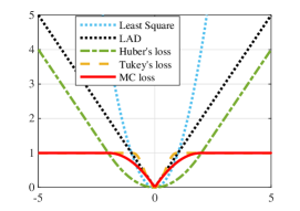
(a) loss function $\phi$

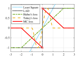
(b) derivative $\psi$

Figure 1: Loss functions and the derivatives (when exist).

II-B1 A tradeoff between robustness and mathematical tractability, and stability aspect

Popular Huber’s loss [5] is more insensitive to outliers than the least square (LS) loss, and it is mathematically tractable owing to its convexity at the same time. Regarding stability with respect to fluctuations caused by Gaussian noise, the Huber’s and LS losses are equally stable. Nevertheless, the robustness of Huber’s loss against huge outliers is limited. This can be seen by inspecting its derivative to which the so-called influence function is proportional [50]. See Fig. 1. It can be seen that the derivative of Huber’s loss stays constant above (or below) the threshold. This means that large outliers give a constant amount of influence to the estimate, thus causing extra estimation bias.

In contrast, Tukey’s biweight loss [51] has a “redescending property (vanishing derivative)”; i.e., the derivative vanishes at some point on each side of the real line. This implies that such outliers that have magnitudes exceeding the threshold would give no influence to the estimate, thus leading to remarkable robustness to huge outliers. Unfortunately, however, Tukey’s biweight is mathematically intractable owing to its nonconvexity. So, how can we break the tradeoff between robustness against huge outliers and mathematical tractability.

To find an answer to this question, let us consider the following question first: can we find such a convex loss that has a vanishing derivative (for sufficiently large values)? This is hopeless actually in a certain sense. To be precise, we restrict ourselves to such a class of loss functions $\phi:{\mathbb{R}}\rightarrow[0,+\infty)$ such that (i) $\phi(0)=0$, (ii) $\phi(e)>0$ if $e\neq 0$, and (iii) $\phi$ is differentiable everywhere but the origin. (This assumption is reasonably mild. See, e.g., [52].) Within this class of functions, $\phi$ is continuous if it is convex, because ${\rm range}\ (\phi)=[0,+\infty)\subset{\mathbb{R}}$ owing to conditions (i) and (iii). In fact, no convex loss has a vanishing derivative in this case. The derivative $\psi:=\phi^{\prime}$ of $\phi$ has the following properties: (i) $\psi(0)=0$ if $\phi$ is also differentiable at $e=0$ which minimizes $\phi$ (or $0\in\partial\phi(0)$ in general), and (ii) $\psi(e)>0$ when $e$ increases from zero infinitesimally. Hence, there is no way for $\psi$ to vanish again because the derivative of a convex function is monotonically non-decreasing.

The above arguments encourage us to explore nonconvex loss functions. In fact, the MC loss $\Phi_{\gamma}^{\rm MC}$ has a vanishing derivative (as can be seen from Fig. 1), and it is mathematically tractable at the same time. Let us now highlight the behaviour of the derivative $\psi$ for each loss in the vicinity of the origin. It can be seen that the derivative vanishes at the origin for the Huber, Tukey’s biweight, and LS losses, while it does not vanish for the MC and LAD losses. This implies a direct use of the MC loss may cause instability with respect to small fluctuations generated by Gaussian noise. We therefore present another formulation using an additional variable vector to model the Gaussian noise vector $\varepsilon_{\star}$ in the following.

II-B2 Stable outlier-robust regression

We introduce the variable vector $\varepsilon\in{\mathbb{R}}^{m}$ to model the noise $\varepsilon_{\star}$. The SORR formulation is given as follows:

$$\min_{x\in{\mathbb{R}}^{n},\varepsilon\in{\mathbb{R}}^{m}}~{} \mu\underbrace{[\left\|y-(Ax+\varepsilon)\right\|_{1}-~{}^{\gamma}\left\|\cdot\right\|_{1}(y-(Ax+\varepsilon))]}_{\Phi_{\gamma}^{\rm MC}(y-(Ax+\varepsilon))}$$

$$+0.5\sigma_{x}^{-2}\left\|x\right\|_{2}^{2}+0.5\sigma_{\varepsilon}^{-2}\left\|\varepsilon\right\|_{2}^{2},$$ (8)

where $\sigma_{x}^{2}\in{\mathbb{R}}_{++}$ and $\sigma_{\varepsilon}^{2}\in{\mathbb{R}}_{++}$ are estimates of $\sigma_{x_{\star}}^{2}$ and $\sigma_{\varepsilon_{\star}}^{2}$, respectively. If such estimates are unavailable, $\sigma_{x}^{2}$ and $\sigma_{\varepsilon}^{2}$ are considered as tuning parameters. An extreme case of SORR with $\sigma_{\varepsilon}\downarrow 0$ (or with a sufficiently small $\sigma_{\varepsilon}>0$) make the optimal $\varepsilon$ of (8) be the zero vector, reducing SORR to the following simple formulation:

$$\min_{x\in{\mathbb{R}}^{n}}~{}\mu\underbrace{[\left\|Ax-y\right\|_{1}-~{}^{\gamma}\left\|\cdot\right\|_{1}(Ax-y)]}_{\Phi_{\gamma}^{\rm MC}(Ax-y)}+0.5\left\|x\right\|_{2}^{2}.$$ (9)

We shall refer to the formulation in (9) as outlier-robust regression (ORR).

The first term $\Phi_{\gamma}^{\rm MC}(y-(Ax+\varepsilon))$ of (8) is the MC loss encouraging sparsity of the estimation residual $y-(Ax+\varepsilon)$ which can be regarded as an estimate of the sparse outlier. The last two terms $0.5\sigma_{x}^{-2}\left\|x\right\|_{2}^{2}$ and $0.5\sigma_{\varepsilon}^{-2}\left\|\varepsilon\right\|_{2}^{2}$ reflect the Gaussianity of $x_{\star}$ and $\varepsilon_{\star}$, playing double roles of convexification and regularization (in the Tikhonov sense). In particular, when the noise power $\sigma_{\varepsilon_{\star}}^{2}$ is large, $\left\|\varepsilon_{\star}\right\|^{2}$ tends to be large as well. In this case, the inverse $\sigma_{\varepsilon}^{-2}$ of the noise-power estimate would be small, and it allows $\left\|\varepsilon\right\|_{2}^{2}$ to be large so that $\varepsilon$ mimics $\varepsilon_{\star}$ well, yielding efficient mitigation of the MC loss $\Phi_{\gamma}^{\rm MC}(y-(Ax+\varepsilon))$. This leads to the “stability” of the SORR estimator in the spirit of [36]. A primal-dual splitting algorithm which can solve some class of linearly-involved nonsmooth convex optimization problems including (8) will be presented in Section III-D. The algorithm relies on convexity of the smooth part of the objective function in (8), for which the condition is given below.

Proposition 3 (Convexity condition for SORR (8))

The smooth part $0.5\sigma_{x}^{-2}\left\|x\right\|_{2}^{2}+0.5\sigma_{\varepsilon}^{-2}\left\|\varepsilon\right\|_{2}^{2}-\mu\hskip 3.00003pt^{\gamma}\left\|\cdot\right\|_{1}(y-(Ax+\varepsilon))$ is convex in $(x,\varepsilon)\in{\mathbb{R}}^{n}\times{\mathbb{R}}^{m}$ if and only if

$$\mu(\sigma_{\varepsilon}^{2}+\sigma_{x}^{2}\lambda_{\max}(A^{\top}A))\leq\gamma.$$ (10)

Proof.

The proof is based on the results to be presented in Section III-C, and it is given in Appendix B. ∎

Remark 4 (SORR resolves the tradeoff efficiently)

The SORR estimator breaks the tradeoff between robustness and mathematical tractability. In particular, SORR enjoys (i) remarkable robustness against huge outliers and (ii) insensitivity to small fluctuations, while the posed problem in (8) is still tractable because the whole cost is convex under (10). Those advantages come mainly from the use of the MC loss and the additional vector $\varepsilon$.

We mention that the introduction of the additional vector $\varepsilon$ does not increase computational complexity essentially, although a larger amount of memory is required than the case of ORR (the $\varepsilon$-parameter free formulation) to store the length-$(n+m)$ vector $\xi$ as well as some other intermediate vectors that are required in the algorithm (see [37] or Section III-D2). Specifically, the algorithm iteration to compute the SORR estimator requires $O(mnQ)$ complexity, in addition to the computation of the largest eigenvalue of $A^{\top}A$ (or $AA^{\top}$) as preprocessing, where $Q$ is the number of iterations.

The SORR formulation has been extended to sparse modeling under Gaussian and impulsive noises [54].

III LiMES Model: Convexity Condition, Algorithm, and Applications

To give the convexity conditions for the debiased sparse modeling and SORR in a unified way, we present a generalized model called “LiMES” and show the necessary and sufficient condition for its convexity. Applications of the LiMES model can be classified into two categories: type-sparse and type-robust. We derive the proximal debiasing-gradient algorithm (which requires no auxiliary variable) for the former type and the primal-dual debiasing algorithm for the latter type. We finally give a couple of other applications than debiased sparse modeling and SORR.

Let $\mathfrak{L}:{\mathcal{H}}\rightarrow{\mathcal{K}}$ be a bounded linear operator from a Hilbert space ${\mathcal{H}}$ to another Hilbert space ${\mathcal{K}}$. The adjoint operator of $\mathfrak{L}$ is denoted by $\mathfrak{L}^{*}$. The operator norm is then defined by $\left\|\mathfrak{L}\right\|:=\sup\{\left\|\mathfrak{L}x\right\|\mid x\in{\mathcal{H}},\left\|x\right\|\leq 1\}$. Given a bounded linear operator $\mathfrak{L}:{\mathcal{H}}\rightarrow{\mathcal{H}}$, $\mathfrak{L}\succeq O$ means that $\mathfrak{L}$ is positive semidefinite, i.e., $\left\langle{\mathfrak{L}x},{x}\right\rangle\geq 0$ for all $x\in{\mathcal{H}}$. Given any bijective bounded linear operator $\mathfrak{L}:{\mathcal{H}}\rightarrow{\mathcal{H}}$ and any function $f\in{\Gamma_{0}(\mathcal{H})}$, it holds that

$$(f\circ\mathfrak{L})^{*}=f^{*}\circ(\mathfrak{L}^{*})^{-1}.$$ (11)

III-A LiMES: A class of weakly convex functions

Definition 1 (The LiMES Model)

Let ${\mathcal{X}}$, ${\mathcal{Y}}$, and ${\mathcal{Z}}$ be finite-dimensional Hilbert spaces. Let ${\mathscr{A}}_{1}:{\mathcal{X}}\rightarrow{\mathcal{Y}}:x\mapsto M_{1}x+c_{1}$ and $\mu\in{\mathbb{R}}_{++}$, where $(O\neq)M_{1}:{\mathcal{X}}\rightarrow{\mathcal{Y}}$ is a bounded linear operator and $c_{1}\in{\mathcal{Y}}$ is a vector. Let $(O\neq)$ $\mathscr{L}:{\mathcal{Z}}\rightarrow{\mathcal{Z}}$ be a bounded linear operator, $D:{\mathcal{Z}}\rightarrow{\mathcal{Z}}$ be a diagonal positive-definite operator, and ${\mathscr{A}}_{2}:{\mathcal{X}}\rightarrow{\mathcal{Z}}:x\mapsto M_{2}x+c_{2}$, where $(O\neq)M_{2}:$ ${\mathcal{X}}\rightarrow{\mathcal{Z}}$ is a bounded linear operator and $c_{2}\in{\mathcal{Z}}$ is a vector. Let $\Psi\in\Gamma_{0}({\mathcal{Z}})$, which is referred to as a seed function. The linearly-involved Moreau-enhanced-over-subspace (LiMES) model is defined as the minimization of the following function:

$$J_{\Omega}:{\mathcal{X}}\rightarrow(-\infty,\infty]:x\mapsto 0.5\left\|{\mathscr{A}}_{1}x\right\|^{2}+\mu\Psi_{D}^{\mathscr{L}}({\mathscr{A}}_{2}x),$$ (12)

where $\Omega:=({\mathscr{A}}_{1};\Psi_{D}^{\mathscr{L}}\circ{\mathscr{A}}_{2})$, and

$$\Psi_{D}^{\mathscr{L}}: ~{}{\mathcal{Z}}\rightarrow(-\infty,+\infty]$$

$$: ~{}z\mapsto\Psi(z)-\min_{v\in{\mathcal{Z}}}\big{[}\Psi(v)+0.5\left\|D(\mathscr{L}z-v)\right\|^{2}\big{]}.$$ (13)

We refer to $\Psi_{D}^{\mathscr{L}}\circ{\mathscr{A}}_{2}:{\mathcal{X}}\rightarrow(-\infty,+\infty]$ as the LiMES function.

Define the subspace $\mathcal{M}_{1}:={\rm range}\hskip 1.99997ptM_{1}^{*}$. The debiased sparse modeling in (4) is reproduced by letting ${\mathcal{X}}:={\mathcal{Z}}:={\mathbb{R}}^{n}$, ${\mathcal{Y}}:={\mathbb{R}}^{m}$, ${\mathscr{A}}_{1}:=A\cdot-y$ ($M_{1}:=A$), $\Psi:=\left\|\cdot\right\|_{1}$, ${\mathscr{A}}_{2}:=I_{n}$ ($M_{2}:=I_{n}$), $\mathscr{L}:=P_{\mathcal{M}_{1}}=P_{\mathcal{M}}=A^{\dagger}A\in{\mathbb{R}}^{n\times n}$, and $D:=\gamma^{-1/2}I_{n}$. On the other hand, ORR in (9) is reproduced by letting ${\mathcal{X}}:={\mathcal{Y}}:={\mathbb{R}}^{n}$, ${\mathcal{Z}}:={\mathbb{R}}^{m}$, ${\mathscr{A}}_{1}:=I_{n}$, $\Psi:=\left\|\cdot\right\|_{1}$, ${\mathscr{A}}_{2}:=A\cdot-y$, $\mathscr{L}:=I_{m}$, and $D:=\gamma^{-1/2}I_{m}$. In the former example, here, the quadratic term $0.5\left\|{\mathscr{A}}_{1}x\right\|^{2}$ of (12) represents the data fidelity, and the second term $\mu\Psi_{D}^{\mathscr{L}}({\mathscr{A}}_{2}x)$ represents the penalty. Hereafter, we shall refer to this type as type-sparse, or type-S for short. In the latter example, on the other hand, the roles of the two terms are reversed, and we refer to this type as type-robust, or type-R. As will be seen in Section III-E, SORR in (8) is also a particular example of the LiMES model. Typical roles of the linear/affine operators are summarized in Table II.

TABLE I: Typical roles of linear/affine operators

$\mathscr{L}$ ​​​	preserving the convexity of the smooth term (default: $P_{{\rm range}\hskip 1.39998ptM_{1}^{*}}$)
$D$​ ​​	assigning individual weights to the variables (Section III-F)
${\mathscr{A}}_{1}$​​​	used to define data fidelity for type-S applications
${\mathscr{A}}_{2}$​​​	used to define data fidelity for type-R applications

TABLE II: Mathematical notation

$\iota_{C}$ ​​​	the indicator function of $C$
$\sigma_{C}$ ​​​	the support function of $C$
$f^{*}$ ​​​	the Fenchel conjugate of $f$
$\left\|\cdot\right\|_{*}$ ​​​	the dual norm of $\left\|\cdot\right\|$
${}^{\gamma}f$ ​​​	the Moreau envelope of $f$, e.g., ${}^{\gamma}\left\|\cdot\right\|_{1}$
${\rm Prox}_{f}$ ​​​	the proximity operator w.r.t. $f$
$P_{\mathcal{M}}$ ​​​	the projection operator onto subspace $\mathcal{M}$
$\mathfrak{L}^{*}$ ​​​	the adjoint of linear operator $\mathfrak{L}$
$\Psi_{D}^{\mathscr{L}}$ ​​​	the LiMES function ($\Psi_{D}^{I}=\Psi_{D}$): see (13)
$J_{\Omega}$ ​​​	the LiMES model for $\Omega:=({\mathscr{A}}_{1};\Psi_{D}^{\mathscr{L}}\circ{\mathscr{A}}_{2})$: see (12)

We now discuss an issue related to the overall convexity of the function $J_{\Omega}$ in (12). Due to the nonsingularity of $D$, it can be verified that

$$\Psi_{D}^{\mathscr{L}}(z) =\Psi(z)-\min_{\tilde{v}\in{\mathcal{Z}}}\big{[}\Psi(D^{-1}\tilde{v})+0.5\left\|D\mathscr{L}z-\tilde{v}\right\|^{2}\big{]}$$

$$=\Psi(z)-\hskip 1.00006pt^{1}(\Psi\circ D^{-1})(D\mathscr{L}z)$$ (14)

$$=\Psi(z)-0.5\left\|D\mathscr{L}z\right\|^{2}+\hskip 1.00006pt^{1}(\Psi^{*}\circ D)(D\mathscr{L}z),$$ (15)

where the last equality is verified by (3) and (11) together with the self-adjointness $D^{*}=D$. Here, the first and third terms of (15) are convex functions of $z$. Since convexity is preserved under composition with an affine operator [42, Proposition 8.20], the LiMES function $\Psi_{D}^{\mathscr{L}}\circ{\mathscr{A}}_{2}$ is $\eta$-weakly convex if $0.5\eta\left\|\cdot\right\|^{2}-0.5\left\|\cdot\right\|^{2}\circ D\mathscr{L}{\mathscr{A}}_{2}$ is convex for some $\eta\in{\mathbb{R}}_{++}$, or equivalently if $\eta I-M_{2}^{*}\mathscr{L}^{*}D^{2}\mathscr{L}M_{2}\succeq O~{}(\Leftrightarrow\eta\geq\left\|D\mathscr{L}M_{2}\right\|^{2})$. Substituting (14) into (12) yields the following smooth-nonsmooth separation:

$$J_{\Omega}\!=\!\underbrace{0.5\left\|\cdot\right\|^{2}\circ{\mathscr{A}}_{1}\!-\!\mu~{}^{1}(\Psi\circ D^{-1})\!\circ\!D\mathscr{L}{\mathscr{A}}_{2}}_{=:F~{}{\rm(smooth)}}\!+\!\!\underbrace{\mu\Psi\!\circ\!{\mathscr{A}}_{2}.}_{{\rm nonsmooth}}$$ (16)

Because our algorithms to be presented in Section III-D treat the smooth and nonsmooth terms separately, both of those terms need to be convex for ensuring convergence to a global minimizer. The convexity condition for the smooth part $F$ will be discussed in Section III-C, as the nonsmooth term is automatically convex due to the convexity of $\Psi$.

For consistent notation with [26], $\Psi_{D}:=\Psi_{D}^{I}$ will be used when $\mathscr{L}:=I$. The question now is: what is the role of the term $\min_{v\in{\mathcal{Z}}}\big{[}\Psi(v)+0.5\left\|D(\mathscr{L}z-v)\right\|^{2}\big{]}$ in (13)? The following proposition, which generalizes Proposition 1, answers this question for the case of $\mathscr{L}:=P_{\mathcal{M}_{1}}$.

Proposition 4

1. The particular LiMES function $\Phi_{\gamma}^{P_{\mathcal{M}_{1}}}$ coincides with the generalized Moreau enhanced penalty $\Psi_{D}$ [26] on the subspace $\mathcal{M}_{1}$; i.e., $\Psi_{D}^{P_{\mathcal{M}_{1}}}(z)=\Psi_{D}^{I}(z)=\Psi_{D}(z)=\Psi(z)-\min_{v\in{\mathcal{Z}}}\big{[}\Psi(v)+0.5\left\|D(z-v)\right\|^{2}\big{]}$ for $z\in\mathcal{M}_{1}$.

2. Let $\mathscr{L}$ satisfy $\mathscr{L}=\mathscr{L}\circ P_{\mathcal{M}_{1}}$. Then, $\Phi_{\gamma}^{\mathscr{L}}$ reduces to $\Psi$ (up to constant) on $\mathcal{M}_{1}^{\perp}$; i.e., $\Psi_{D}^{\mathscr{L}}(z)=\Psi(z)-\underbrace{\min_{v\in{\mathcal{Z}}}\big{[}\Psi(v)+0.5\left\|Dv\right\|^{2}\big{]}}_{{\rm constant~{}in~{}}z}$ for $z\in\mathcal{M}_{1}^{\perp}$.

Proof.

(a) The assertion can be verified by applying $P_{\mathcal{M}_{1}}z=z$ for all $z\in\mathcal{M}_{1}$ to (14) with $\mathscr{L}:=P_{\mathcal{M}_{1}}$.
(b) Use $\mathscr{L}z=\mathscr{L}\circ P_{\mathcal{M}_{1}}z=\mathscr{L}0=0$, $\forall z\in\mathcal{M}_{1}^{\perp}$ in (13). ∎

Proposition 4 states, under the use of $\mathscr{L}:=P_{\mathcal{M}_{1}}$, that $\Psi_{D}^{P_{\mathcal{M}_{1}}}$ is an “exact” Moreau-enhanced model over the subspace $\mathcal{M}_{1}$ in the sense of the generalized Moreau enhanced (GME) penalty [26]. Note here that $\min_{v\in{\mathcal{Z}}}\big{[}\Psi(v)+0.5\left\|D(z-v)\right\|^{2}\big{]}$ can be regarded as a generalized Moreau envelope of $\Psi$. In all applications presented in this article, $\mathscr{L}:=P_{\mathcal{M}_{1}}$ will be used. Nevertheless, we would not exclude the possibility of using other choices of $\mathscr{L}$ such as those presented in [25, 26], although the Moreau enhancement over $\mathcal{M}_{1}$ could be “inexact” in this case (see Example 1 in Section III-B). Proposition 4(b) states that $\Psi_{D}^{\mathscr{L}}$ coincides with $\Psi$ over $\mathcal{M}_{1}^{\perp}$ up to constant under the condition (which $\mathscr{L}:=P_{\mathcal{M}_{1}}$ satisfies).

As shown in Section II-A, the PMC penalty preserves the convexity of the smooth part even when $A^{\top}A$ is singular, and at the same time it enjoys the mixed nature of separability and nonseparability. Such a penalty can be generated systematically by the LiMES function with $\mathscr{L}:=P_{\mathcal{M}_{1}}$ given a separable function $\Psi$. We emphasize here that the diagonality of $D$ induces the separability of the function $\Psi(v)+0.5\left\|D(\mathscr{L}z-v)\right\|^{2}$ in (13) in terms of $v$, which makes the gradient computation of the smooth part $F$ in (16) simple (see Remark 1). In particular, for typical type-S applications (such as debiased sparse modeling and SPCP to be presented in Section III-F), ${\mathscr{A}}_{2}$ is also a diagonal operator, and thus the computationally efficient proximal gradient algorithm can be applied which requires no auxiliary vector to compute the LiMES model (see Section III-D).

To show an active role of the diagonal operator $D$ briefly, suppose that the variable vector $x\in{\mathcal{X}}$ consists of several subvectors. In this case, $D$ can be used to give an individual weight to the regularizer of each subvector (see Section III-F).

III-B Examples of LiMES function: penalty and loss

In this subsection, we simply let $D:=\gamma^{-1/2}I$ for $\gamma\in{\mathbb{R}}_{++}$, which reduces (14) to

$$\Psi_{D}^{\mathscr{L}}(z)=\Psi_{\gamma^{-1/2}I}^{\mathscr{L}}(z)=\Psi(z)-\hskip 1.00006pt^{\gamma}\Psi(\mathscr{L}z).$$ (17)

Some examples of the LiMES function are listed below.

Example 1 (LiMES penalty)

We let ${\mathcal{X}}:={\mathbb{R}}^{n}$ and ${\mathcal{Z}}:={\mathbb{R}}^{m}$ in (a) – (d) below.

1. (MC penalty [17, 27]) Let $\Psi:=\left\|\cdot\right\|_{1}$, $\mathscr{L}:={\mathscr{A}}_{2}:=I_{n}$ ($n=m$). Then, $(\left\|\cdot\right\|_{1})_{\gamma^{-1/2}I}:=\left\|\cdot\right\|_{1}-^{\gamma}\left\|\cdot\right\|_{1}=\Phi_{\gamma}^{\rm MC}$. In particular, the MC penalty, or $\theta_{\gamma}(\left\|\cdot\right\|_{1})_{\gamma^{-1/2}I}$ more specifically, gives a parametric bridge between $\left\|\cdot\right\|_{0}$ and $\left\|\cdot\right\|_{1}$ [26] (see Remark 2 for definition of $\theta_{\gamma}$).

2. (PME and PMC) Let $\mathscr{L}:=P_{\mathcal{M}_{1}}$ and ${\mathscr{A}}_{2}:=I_{n}$ ($n=m$), where $\mathcal{M}_{1}\subset{\mathbb{R}}^{n}$ is a linear subspace of ${\mathbb{R}}^{n}$. Then, $\Psi_{\gamma^{-1/2}I}^{P_{\mathcal{M}_{1}}}=\Psi-\hskip 1.00006pt^{\gamma}\Psi~{}\circ~{}P_{\mathcal{M}_{1}}$, which we call the projective Moreau enhanced (PME) function. In particular, letting $\Psi:=\left\|\cdot\right\|_{1}$ yields $(\left\|\cdot\right\|_{1})_{\gamma^{-1/2}I}^{P_{\mathcal{M}_{1}}}:=\left\|\cdot\right\|_{1}-^{\gamma}\left\|\cdot\right\|_{1}\circ P_{\mathcal{M}_{1}}=\Phi_{\gamma}^{\rm PMC}$, which is the PMC penalty presented in Section II-A. An alternative choice of $\mathscr{L}$ to the $P_{\mathcal{M}_{1}}$ used in $\Phi_{\gamma}^{\rm PMC}$ is given by $\mathscr{L}:=\sqrt{\gamma/\mu}V{\rm diag}(\alpha_{1}^{1/2},\alpha_{2}^{1/2},\cdots,\alpha_{n}^{1/2})\Sigma_{A^{\top}A}^{1/2}V^{\top}$ (cf. [25]), where $\alpha_{i}\in[0,1]$, $i=1,2,\cdots,n$, are tuning parameters, and $A^{\top}A=V\Sigma_{A^{\top}A}V^{\top}$ is an eigenvalue decomposition with some orthogonal matrix $V\in{\mathbb{R}}^{n\times n}$ and some diagonal matrix $\Sigma_{A^{\top}A}\succeq O$. (This choice actually satisfies the convexity condition to be presented in Section III-C.)

3. (MC-W) Let $\Psi:=\left\|\cdot\right\|_{1}$, $\mathscr{L}:=I_{n}$ ($n=m$), and ${\mathscr{A}}_{2}:=\mathscr{W}$, where $\mathscr{W}$ is the popular wavelet transform [58]. Then, $(\left\|\cdot\right\|_{1})_{\gamma^{-1/2}I}\circ\mathscr{W}$ is the MC wavelet (MC-W).

4. (MC-TV) Let $\Psi:=\left\|\cdot\right\|_{1}$, $\mathscr{L}:=I_{n-1}$ ($m=n-1$), and ${\mathscr{A}}_{2}:=\mathscr{D}_{n}:=[0_{n-1}~{}I_{n-1}]-[I_{n-1}~{}0_{n-1}]\in{\mathbb{R}}^{(n-1)\times n}$ be the first-order differential operator, where $0_{n}:=[0,0,\cdots,0]^{\top}\in{\mathbb{R}}^{n}$ for any $n\in{\mathbb{N}}^{*}$. Then, $(\left\|\cdot\right\|_{1})_{\gamma^{-1/2}I}\circ\mathscr{D}_{n}$ has been used in MC total-variation (MC-TV) denoising [59].

5. (MEN) Let ${\mathcal{X}}:={\mathcal{Z}}:={\mathbb{R}}^{n\times m}$, and $\Psi:=\left\|\cdot\right\|_{\rm nuc}$, which is the nuclear norm (the sum of the singular values) of a matrix, and $\mathscr{L}:={\mathscr{A}}_{2}:=I$. Then, $(\left\|\cdot\right\|_{\rm nuc})_{\gamma^{-1/2}I}$ gives the Moreau enhanced nuclear-norm (MEN). In particular, the normalized version $2\gamma^{-1}(\left\|\cdot\right\|_{\rm nuc})_{\gamma^{-1/2}I}$ gives a parametric bridge between the rank of matrix and $\left\|\cdot\right\|_{\rm nuc}$ [26]. The MEN penalty will be used in Section III-F for SPCP.

Example 2 (LiMES loss)

We let ${\mathcal{X}}:={\mathbb{R}}^{n}$ and ${\mathcal{Z}}:={\mathbb{R}}^{m}$ in (a) – (c) below, and $A\in{\mathbb{R}}^{m\times n}$ and $y\in{\mathbb{R}}^{m}$ in (a), (c), and (d).

1. (MC loss) Let $\Psi:=\left\|\cdot\right\|_{1}$, $\mathscr{L}:=I_{m}$, and ${\mathscr{A}}_{2}:{\mathbb{R}}^{n}\rightarrow{\mathbb{R}}^{m}:x\mapsto Ax-y$. Then, $(\left\|\cdot\right\|_{1})_{\gamma^{-1/2}I}(A\cdot-y)=\Phi_{\gamma}^{\rm MC}(A\cdot-y)$ gives an MC loss, which has been studied in Section II-B for robust regression.

2. (ME-hinge loss) Let $\Psi:=\sigma_{[-1,0]}:{\mathbb{R}}\rightarrow{\mathbb{R}}:z\mapsto\sup_{v\in[-1,0]}vz=\max\{0,-z\}$, $\mathscr{L}:=I_{m}=1$ ($m:=1$), and ${\mathscr{A}}_{2}:{\mathbb{R}}^{n}\rightarrow{\mathbb{R}}:x\mapsto a^{\top}x-1$ for some given $a\in{\mathbb{R}}^{n}$ such that $\left\|a\right\|_{2}=1$. Then, $\Psi_{\rm hinge}:=\Psi\circ{\mathscr{A}}_{2}:{\mathcal{X}}\rightarrow{\mathbb{R}}:x\rightarrow\max\{0,1-a^{\top}x\}$ is the hinge loss function, and we call $(\Psi_{\rm hinge})_{\gamma^{-1/2}I}=\Psi_{\gamma^{-1/2}I}\circ{\mathscr{A}}_{2}$ the Moreau-enhanced hinge (ME-hinge) loss function. See Proposition 7 for the second equality here. The proximity operator of $\Psi_{\rm hinge}$ is given for instance in [42, Example 24.37]. The ME-hinge loss will be used in Section III-G for robust classification.

3. (MC-W loss) Let $\Psi:=\left\|\cdot\right\|_{1}$, $\mathscr{L}:=I_{m}$, and ${\mathscr{A}}_{2}:{\mathbb{R}}^{n}\rightarrow{\mathbb{R}}^{m}:x\mapsto\mathscr{W}(Ax-y)$. Then, $(\left\|\cdot\right\|_{1})_{\gamma^{-1/2}I}(\mathscr{W}(A\cdot-y))$ gives an MC-W loss.

4. (MC-TV loss) Let ${\mathcal{X}}:={\mathbb{R}}^{n}$, ${\mathcal{Z}}:={\mathbb{R}}^{m-1}$, $\Psi:=\left\|\cdot\right\|_{1}$, $\mathscr{L}:=I_{m-1}$, and ${\mathscr{A}}_{2}:{\mathbb{R}}^{n}\rightarrow{\mathbb{R}}^{m-1}:x\mapsto\mathscr{D}_{m}(Ax-y)$. Then, $(\left\|\cdot\right\|_{1})_{\gamma^{-1/2}I}(\mathscr{D}_{m}(A\cdot-y))$ gives an MC-TV loss.

5. (MEN loss) Let ${\mathcal{X}}:={\mathcal{Z}}:={\mathbb{R}}^{n\times m}$, $\Psi:=\left\|\cdot\right\|_{\rm nuc}$, $\mathscr{L}:=I$, and ${\mathscr{A}}_{2}:{\mathbb{R}}^{n\times m}\rightarrow{\mathbb{R}}^{n\times m}:X\mapsto X-Y$ given $Y\in{\mathbb{R}}^{n\times m}$. Then, $(\left\|\cdot\right\|_{\rm nuc})_{\gamma^{-1/2}I}\circ(\cdot-Y)$ gives a MEN loss.

III-C Convexity condition for the smooth part of (16)

We discuss the condition for convexity of the smooth part $F$, which immediately implies the overall convexity of $J_{\Omega}$ since the nonsmooth term $\mu\Psi\circ{\mathscr{A}}_{2}$ is clearly convex. By (14) and (15), the smooth part of (16) can be rewritten as

$$F=0.5(\left\|{\mathscr{A}}_{1}\cdot\right\|^{2}-\mu\left\|D\mathscr{L}{\mathscr{A}}_{2}\cdot\right\|^{2})+\mu\hskip 3.00003pt^{1}(\Psi^{*}\circ D)\circ D\mathscr{L}{\mathscr{A}}_{2}.$$ (18)

Since the third term here is automatically convex, $F$ is convex if the sum of the first two terms is convex; i.e., $F$ is convex if

$$(\spadesuit)~{}~{}~{}M_{1}^{*}M_{1}-\mu M_{2}^{*}\mathscr{L}^{*}D^{2}\mathscr{L}M_{2}\succeq O.$$

In general, ($\spadesuit$) is not a necessary condition. When the third term of (18) is strongly convex, for instance, $F$ could be convex even if $0.5\left\|{\mathscr{A}}_{1}\cdot\right\|^{2}-0.5\mu\left\|D\mathscr{L}{\mathscr{A}}_{2}\cdot\right\|^{2}$ is nonconvex. It can actually be observed that the function ${}^{1}(\Psi^{*}\circ D)$ is strongly convex if and only if $\Psi$ is smooth (i.e., Fréchet differentiable with Lipschitz-continuous gradient) due to [42, Theorem 18.15] together with $(^{1}(\Psi^{*}\circ D))^{*}=\Psi^{**}\circ D^{-1}+0.5\left\|\cdot\right\|^{2}=\Psi\circ D^{-1}+0.5\left\|\cdot\right\|^{2}$ [42, Proposition 13.24]. Typical seed functions $\Psi$ including those presented in Section III-B are nonsmooth, and the above observation indicates that the third term of (18) is not strongly convex for such nonsmooth $\Psi$s. In fact, ($\spadesuit$) is a necessary and sufficient condition in those cases as well as many other cases.

To present the formal result regarding the convexity condition for $F$, we define the support function $\Gamma_{0}({\mathcal{Z}})\ni\sigma_{C}:z\mapsto\sup_{v\in C}\left\langle{z},{v}\right\rangle$ of a nonempty closed convex set $C\subset{\mathcal{Z}}$, which is the conjugate function of the indicator function $\Gamma_{0}({\mathcal{Z}})\ni\iota_{C}:z\mapsto\left\{\begin{array}[]{cc}0&\mbox{ if }z\in C\\ +\infty&\mbox{ if }z\not\in C,\end{array}\right.$ and hence $\sigma_{C}^{*}=\iota_{C}^{**}=\iota_{C}$. Given an arbitrary norm $|||\cdot|||$ defined on the vector space ${\mathcal{Z}}$, the support function $|||\cdot|||_{*}:=\sigma_{C}$ of its level set $C:={\rm lev}_{\leq 1}|||\cdot|||$ is the dual norm of $|||\cdot|||$ [60, 61]. It is known that the dual of the dual norm is the original norm, i.e., $|||\cdot|||_{**}=|||\cdot|||$. An arbitrary norm defined on ${\mathcal{Z}}$ can therefore be represented as the support function of the level set of its dual norm.

Given any bounded linear operator $\mathfrak{L}:{\mathcal{H}}\rightarrow{\mathcal{K}}$ from a Hilbert space ${\mathcal{H}}$ to another Hilbert space ${\mathcal{K}}$ and any subsets $C_{{\mathcal{H}}}\subset{\mathcal{H}}$ and $C_{{\mathcal{K}}}\subset{\mathcal{K}}$, we define $\mathfrak{L}(C_{{\mathcal{H}}}):=\{\mathfrak{L}x\mid x\in C_{{\mathcal{H}}}\}\subset{\mathcal{K}}$ and $\mathfrak{L}^{-1}(C_{{\mathcal{K}}}):=\{x\in{\mathcal{H}}\mid\mathfrak{L}x\in C_{{\mathcal{K}}}\}$.

Proposition 5 (Convexity condition for smooth part of (16))

1. $F\in\Gamma_{0}({\mathcal{X}})$ if condition ($\spadesuit$) is satisfied.

2. Let $\Psi:=\sigma_{C}$ with a nonempty closed convex set $C\subset{\mathcal{Z}}$. Then, the following statements hold.

   1. Given any $x\in{\mathcal{X}}$, the following equivalence holds:

      $$~{}F(x)=0.5\left\|{\mathscr{A}}_{1}x\right\|^{2}-0.5\mu\left\|D\mathscr{L}{\mathscr{A}}_{2}x\right\|^{2}$$

      $$\Leftrightarrow ~\hskip 1.00006pt{}^{1}(\sigma_{C}^{*}\circ D)(D\mathscr{L}{\mathscr{A}}_{2}x)=0$$

      $$\Leftrightarrow ~{}x\in K_{C}:=\{\hat{x}\in{\mathcal{X}}\mid D^{2}\mathscr{L}{\mathscr{A}}_{2}\hat{x}\in C\}.$$ (19)

   2. Assume that

      $${\rm int}\hskip 1.99997ptK_{C}\neq\emptyset,$$ (20)

      where ${\rm int}\hskip 1.99997ptK_{C}$ is the interior of $K_{C}$. Then, $F\in\Gamma_{0}({\mathcal{X}})$ if and only if ($\spadesuit$) is satisfied.

Proof.

(a) It is clear under ($\spadesuit$) that $0.5\left\|{\mathscr{A}}_{1}\cdot\right\|^{2}-0.5\mu\left\|D\mathscr{L}{\mathscr{A}}_{2}\cdot\right\|^{2}\in\Gamma_{0}({\mathcal{X}})$. It can also be verified that $\Psi\in\Gamma_{0}({\mathcal{X}})\Rightarrow\Psi^{*}\in\Gamma_{0}({\mathcal{X}})\Rightarrow^{1}(\Psi^{*}\circ D)\circ D\mathscr{L}{\mathscr{A}}_{2}\in\Gamma_{0}({\mathcal{X}})$.

(b.i) For $v\in{\mathcal{Z}}$, it can be verified that

$${}^{1}(\sigma_{C}^{*}\circ D)(v)= ~{}\min_{z\in{\mathcal{Z}}}~{}\left[\iota_{C}(Dz)+0.5\left\|v-z\right\|^{2}\right]$$

$$= ~{}\!\!\min_{z\in D^{-1}(C)}\!0.5\left\|v-z\right\|^{2}=:0.5d^{2}(v,D^{-1}(C)).$$

It follows thus that  ${}^{1}(\sigma_{C}^{*}\circ D)\circ D\mathscr{L}{\mathscr{A}}_{2}=0.5d^{2}(D\mathscr{L}{\mathscr{A}}_{2}\cdot,D^{-1}(C))$, and using this equality in (18) verifies that $F(x)=0.5\left\|{\mathscr{A}}_{1}x\right\|^{2}-0.5\mu\left\|D\mathscr{L}{\mathscr{A}}_{2}x\right\|^{2}\Leftrightarrow\hskip 1.00006pt^{1}(\sigma_{C}^{*}\circ D)(D\mathscr{L}{\mathscr{A}}_{2}x)=0\Leftrightarrow D\mathscr{L}{\mathscr{A}}_{2}x\in D^{-1}(C)\Leftrightarrow D^{2}\mathscr{L}{\mathscr{A}}_{2}x\in C\Leftrightarrow x\in K_{C}$.

(b.ii) Since the third term of (18) vanishes over ${\rm int}\hskip 1.99997ptK_{C}\neq\emptyset$ by Proposition 5(b.i), $F$ is nonconvex if condition ($\spadesuit$) is unsatisfied. This implies the necessity of ($\spadesuit$). The sufficiency is verified already in Proposition 5(a). ∎

Proposition 5 shows the situation under which ($\spadesuit$) is a necessary and sufficient condition. The necessity implies that the condition cannot be weaker, or, in other words, the parameter $\mu$ cannot exceed the upper bound obtained from ($\spadesuit$). We remark that the diagonality and positive definiteness imposed implicitly on $D$ in Proposition 5 can be relaxed straightforwardly by solely imposing bijectivity.

Lemma 1

Let $\mathfrak{L}:{\mathcal{X}}\rightarrow{\mathcal{Z}}$ be a bounded linear operator. Given a nonempty set $(\emptyset\neq)C\subset{\mathcal{Z}}$ and a point $\hat{x}\in{\mathcal{X}}$, it holds that $\mathfrak{L}\hat{x}\in{\rm int}\hskip 1.99997ptC$ implies $\hat{x}\in{\rm int}\hskip 1.99997pt\mathfrak{L}^{-1}(C)$. If $\mathfrak{L}$ is surjective, $\mathfrak{L}\hat{x}\in{\rm int}\hskip 1.99997ptC\Leftrightarrow\hat{x}\in{\rm int}\hskip 1.99997pt\mathfrak{L}^{-1}(C)$.

Proof.

We denote by $\mathcal{B}(x,\epsilon):=\{u\in{\mathcal{X}}\mid\left\|u-x\right\|<\epsilon\}$ an open ball centered at $x\in{\mathcal{X}}$ with radius $\epsilon\in{\mathbb{R}}_{++}$. Assume that $\mathfrak{L}\hat{x}\in{\rm int}\hskip 1.99997ptC$. Then, there exists some $\epsilon\in{\mathbb{R}}_{++}$ such that $\mathcal{B}(\mathfrak{L}\hat{x},\epsilon)\subset C$. It can then be shown straightforwardly that $\mathcal{B}(\hat{x},\epsilon/\left\|\mathfrak{L}\right\|)\subset\mathfrak{L}^{-1}(C)$, and hence $\hat{x}\in{\rm int}\hskip 1.99997pt\mathfrak{L}^{-1}(C)$. The converse implication in the equivalence part is an implication of the well-known open mapping theorem [62]. To see this, assume that $\mathfrak{L}$ is surjective and that $\hat{x}\in{\rm int}\hskip 1.99997pt\mathfrak{L}^{-1}(C)$. Then, there exists an $\epsilon\in{\mathbb{R}}_{++}$ such that $\mathcal{B}(\hat{x},\epsilon)\subset\mathfrak{L}^{-1}(C)$, and the image $\mathfrak{L}(\mathcal{B}(\hat{x},\epsilon))$ is an open set due to the open mapping theorem. The inclusion $\mathfrak{L}\hat{x}\in\mathfrak{L}(\mathcal{B}(\hat{x},\epsilon))\subset C$ due to definition of inverse mapping thus implies $\mathfrak{L}\hat{x}\in{\rm int}\hskip 1.99997pt\mathfrak{L}(\mathcal{B}(\hat{x},\epsilon))\subset{\rm int}\hskip 1.99997ptC$. ∎

The following lemma gives a way of checking the nonemptiness condition of ${\rm int}\hskip 1.99997ptK_{C}$ for necessity in Proposition 5.

Lemma 2

Consider the following statements: (i) ${\rm int}\hskip 1.99997ptK_{C}\neq\emptyset$, (ii) ${\rm int}\hskip 1.99997ptC\neq\emptyset$, and (iii) $D^{2}\mathscr{L}{\mathscr{A}}_{2}\hat{x}\in{\rm int}\hskip 1.99997ptC\neq\emptyset$ for some $\hat{x}\in{\mathcal{X}}$. Then, (iii) $\Rightarrow$ (i). If ${\rm range}\hskip 1.99997pt(\mathscr{L}M_{2})={\mathcal{Z}}$, (i) $\Leftrightarrow$ (ii).

Proof.

By Lemma 1, (iii) $\Rightarrow$ $\exists\hat{x}\in{\mathcal{X}}$, $D^{2}\mathscr{L}M_{2}\hat{x}\in{\rm int}\hskip 1.99997pt(C-D^{2}\mathscr{L}c_{2})$ $\Rightarrow$ $\exists\hat{x}\in{\mathcal{X}}$, $\hat{x}\in{\rm int}\hskip 1.99997pt(D^{2}\mathscr{L}M_{2})^{-1}(C-D^{2}\mathscr{L}c_{2})={\rm int}\hskip 1.99997ptK_{C}$ $\Rightarrow$ (i). Here, $C-D^{2}\mathscr{L}c_{2}:=\{z-D^{2}\mathscr{L}c_{2}\mid z\in C\}\subset{\mathcal{Z}}$. Suppose now that ${\rm range}\hskip 1.99997pt(\mathscr{L}M_{2})={\mathcal{Z}}$. Then, $D^{2}\mathscr{L}M_{2}$ is surjective, and it follows with Lemma 1 that (ii) $\Rightarrow$ (iii) $\Rightarrow$ (i) $\Rightarrow$ $\exists\hat{x}\in{\mathcal{X}}$, $D^{2}\mathscr{L}M_{2}\hat{x}\in{\rm int}\hskip 1.99997pt(C-D^{2}\mathscr{L}c_{2})$ $\Rightarrow$ $\exists\hat{x}\in{\mathcal{X}}$, $D^{2}\mathscr{L}(M_{2}\hat{x}+c_{2})\in{\rm int}\hskip 1.99997ptC$ $\Rightarrow$ (ii). ∎

Combining Proposition 5 and Lemma 2 gives the following corollary.

Corollary 1

Let $\Psi:=|||\cdot|||$. Assume that one of the following conditions are satisfied: (i) $c_{2}=0$, (ii) ${\rm range}\hskip 1.99997ptM_{2}={\mathcal{Z}}$, or (iii) ${\mathscr{A}}_{2}\hat{x}=0$ for some $\hat{x}\in{\mathcal{X}}$. Then, $F\in\Gamma_{0}({\mathcal{X}})$ if and only if condition ($\spadesuit$) is satisfied.

Proof.

As ${\mathscr{A}}_{2}0=c_{2}$, (i) $\Rightarrow$ (iii). Moreover, as ${\mathscr{A}}_{2}\hat{x}=0\Leftrightarrow M_{2}\hat{x}=-c_{2}\in{\mathcal{Z}}$, (ii) $\Rightarrow$ (iii). Since $|||\cdot|||=\sigma_{C}$ for $C:={\rm lev}_{\leq 1}|||\cdot|||_{*}$, it holds that $|||0|||_{*}=0<1\Leftrightarrow 0\in{\rm int}\hskip 1.99997ptC\neq\emptyset$. Hence, (iii) of Corollary 1 $\Rightarrow$ (iii) of Lemma 2 $\Rightarrow{\rm int}\hskip 1.99997ptK_{C}\neq\emptyset$. The assertion is thus verified by Proposition 5. ∎

Corollary 1 is useful when $\Psi$ is a norm, because it gives simple ways of seeing whether ($\spadesuit$) is necessary and sufficient.

III-D Proximal debiasing algorithms

We present iterative algorithms using the proximity operator to compute the LiMES model for the case of $D:=\gamma^{-1/2}I$ for simplicity, which covers many applications including the debiased sparse modeling (4), SORR (8), ORR (9), and robust classification (34) (see Section III-G). (An extension to a general diagonal positive-definite operator $D$ is straightforward.) In this case, (16) reduces to

$$J_{\Omega_{\gamma}}=\underbrace{0.5\left\|{\mathscr{A}}_{1}\cdot\right\|^{2}-\mu\hskip 1.99997pt^{\gamma}\Psi\circ\mathscr{L}{\mathscr{A}}_{2}}_{{\rm smooth}}~{}+~{}\underbrace{\mu\Psi\circ{\mathscr{A}}_{2},}_{{\rm nonsmooth}}$$ (21)

where $\Omega_{\gamma}:=({\mathscr{A}}_{1};\Psi_{\gamma^{-1/2}I}^{\mathscr{L}}\circ{\mathscr{A}}_{2})$. Here, the gradients of $0.5\left\|{\mathscr{A}}_{1}\cdot\right\|^{2}$ and ${}^{\gamma}\Psi\circ\mathscr{L}{\mathscr{A}}_{2}$ at $x\in{\mathcal{X}}$ are given, respectively, by $\nabla(0.5\left\|{\mathscr{A}}_{1}\cdot\right\|^{2})(x)=M_{1}^{*}{\mathscr{A}}_{1}x$ and (see Section I-D)

$$\nabla(^{\gamma}\Psi\!\circ\!\mathscr{L}{\mathscr{A}}_{2})(x)= ~{}M_{2}^{*}\mathscr{L}^{*}\nabla\hskip 3.00003pt^{\gamma}\Psi(\mathscr{L}{\mathscr{A}}_{2}x)$$

$$= ~{}\gamma^{-1}M_{2}^{*}\mathscr{L}^{*}(I-{\rm Prox}_{\gamma\Psi})(\mathscr{L}{\mathscr{A}}_{2}x).$$ (22)

Both gradient operators $\nabla(0.5\left\|{\mathscr{A}}_{1}\cdot\right\|^{2})(x)$ and $\nabla(^{\gamma}\Psi\!\circ\!\mathscr{L}{\mathscr{A}}_{2})$ are Lipschitz continuous with constants $\left\|M_{1}\right\|^{2}$ and $\gamma^{-1}\left\|\mathscr{L}\right\|^{2}\left\|M_{2}\right\|^{2}$, respectively.

III-D1 Proximal debiasing-gradient algorithm for typical type-S applications

Let ${\mathscr{A}}_{2}:=I$ which is used in typical type-S applications. This allows to use an efficient algorithm requiring no auxiliary variable. Specifically, under condition ($\spadesuit$), (21) can be minimized by the proximal gradient method:

$$x_{k+1}\!:= ~{}{\rm Prox}_{\beta_{k}\mu\Psi}[x_{k}\!-\!\beta_{k}(M_{1}^{*}{\mathscr{A}}_{1}x_{k}$$

$$\hskip 10.00002pt-\mu\gamma^{-1}\mathscr{L}^{*}(I-{\rm Prox}_{\gamma\Psi})(\mathscr{L}x))],~{}k\!\in\!{\mathbb{N}},$$ (23)

where $\beta_{k}\in(0,2/(\left\|M_{1}\right\|^{2}+\mu\gamma^{-1}\left\|\mathscr{L}\right\|^{2}))$. ISDA presented in Section II-A4 is reproduced by letting $\Psi:=\left\|\cdot\right\|_{1}$ and $\mathscr{L}:=P_{\mathcal{M}}$ in (23), which makes ${\rm Prox}_{\delta\left\|\cdot\right\|_{1}}={\rm soft}_{\delta}$ for any $\delta\in{\mathbb{R}}_{++}$. The gradient term $\mu\mathscr{L}^{*}\nabla\hskip 3.00003pt^{\gamma}\Psi(\mathscr{L}x_{k})$ actually plays the same role as the “debiasing” term of ISDA. We therefore refer to the algorithm as the proximal debiasing-gradient algorithm.

III-D2 Primal-dual debiasing algorithm for type-R applications

Let $\tilde{\Psi}(z):=\mu\Psi(z+c_{2})$, $z\in{\mathcal{Z}}$, so that $\tilde{\Psi}(M_{2}x)=\mu\Psi({\mathscr{A}}_{2}x)$. The problem in (21) can then be rewritten as

$$\min_{x\in{\mathcal{X}}}~{}0.5\left\|{\mathscr{A}}_{1}x\right\|^{2}-\mu\hskip 1.99997pt^{\gamma}\Psi(\mathscr{L}{\mathscr{A}}_{2}x)~{}+~{}\tilde{\Psi}(M_{2}x).$$ (24)

By ${\rm Prox}_{\tilde{\Psi}/\sigma}(z)=-c_{2}+{\rm Prox}_{\mu\Psi/\sigma}(z+c_{2})$ for $\sigma\in{\mathbb{R}}_{++}$, it follows that

$${\rm Prox}_{\sigma\tilde{\Psi}^{*}}(z)= ~{}z-\sigma{\rm Prox}_{\tilde{\Psi}/\sigma}(\sigma^{-1}z)$$

$$= ~{}z+\sigma c_{2}-\sigma{\rm Prox}_{\mu\Psi/\sigma}(\sigma^{-1}z+c_{2}),$$ (25)

where the first equality is due to the well-known identity [42, Theorem 14.3]: ${\rm Prox}_{\gamma f}+\gamma{\rm Prox}_{f^{*}/\gamma}\circ\gamma^{-1}I=I$ for any $f\in\Gamma_{0}({\mathcal{Z}})$ and $\gamma\in{\mathbb{R}}_{++}$. Problem (24) can be solved by the existing operator splitting methods such as the forward-backward-based primal-dual method [63, 64, 65]; see Algorithm 1 below.

Algorithm 1 (Primal-dual debiasing algorithm)

Set: $x_{0}\in{\mathcal{X}}$, $v_{0}\in{\mathcal{Z}}$, $(\tau,\sigma)\in{\mathbb{R}}_{++}^{2}$, $\beta_{k}\in{\mathbb{R}}_{++}$
For $k=0,1,2,\cdots$, do:
   $s_{k}=x_{k}-\tau[M_{1}^{*}{\mathscr{A}}_{1}x_{k}$
                        $-\mu\gamma^{-1}M_{2}^{*}\mathscr{L}^{*}(I-{\rm Prox}_{\gamma\Psi})(\mathscr{L}{\mathscr{A}}_{2}x_{k})]$
   $u_{k}=s_{k}-\tau M_{2}^{*}v_{k}$
   $q_{k}={\rm Prox}_{\sigma\tilde{\Psi}^{*}}(v_{k}+\sigma M_{2}u_{k})$
   $p_{k}=s_{k}-\tau M_{2}^{*}q_{k}$
   $(x_{k+1},v_{k+1})=(x_{k},v_{k})+\beta_{k}\left((p_{k},q_{k})-(x_{k},v_{k})\right)$

Convergence condition of Algorithm 1: (i) $\tau\sigma\left\|M_{2}\right\|^{2}\in(0,1)$ and $\tau\in(0,2/(\left\|M_{1}\right\|^{2}+\mu\gamma^{-1}\left\|\mathscr{L}M_{2}\right\|^{2}))$, (ii) $(\beta_{k})_{k\in{\mathbb{N}}}\subset(0,1]$ and $\inf_{k\in{\mathbb{N}}}\beta_{k}\in{\mathbb{R}}_{++}$, (iii) the function $J_{\Omega_{\gamma}}$ in (12) has a minimizer, and (iv) ${\rm int}({\rm dom}\hskip 1.99997pt\tilde{\Psi})\cap{\rm range}\hskip 1.99997ptM_{2}\neq\emptyset$.

III-E Stable outlier-robust regression as a special case of LiMES model

We consider a general situation when the augmented vector $\xi_{\star}:=[x_{\star}^{\top}~{}\varepsilon_{\star}^{\top}]^{\top}\in{\mathbb{R}}^{n+m}$ obeys a zero-mean normal distribution with its (nonsingular) covariance matrix $\Sigma_{\xi_{\star}}\in{\mathbb{R}}^{(n+m)\times(n+m)}$. In this case, the standard statistical argument may suggest the use of $0.5\big{\|}\Sigma_{\xi}^{-1/2}\xi\big{\|}_{2}^{2}$, where $\xi:=[x^{\top}~{}\varepsilon^{\top}]^{\top}\in{\mathbb{R}}^{n+m}$ and $\Sigma_{\xi}$ is an estimate of $\Sigma_{\xi_{\star}}$. The estimate $y-(Ax+\varepsilon)=y-[A~{}I_{m}]\xi$ of the sparse outlier is encouraged to be sparse by employing $(\left\|\cdot\right\|_{1})_{\gamma^{-1/2}I}([A~{}I_{m}]\xi-y)$ as a fidelity function. The above arguments amount to the following minimization problem:

$$\min_{\xi\in{\mathbb{R}}^{n+m}}0.5\big{\|}\underbrace{\Sigma_{\xi}^{-1/2}\xi}_{=:{\mathscr{A}}_{1}\xi}\big{\|}_{2}^{2}+~{}\mu(\underbrace{\left\|\cdot\right\|_{1}}_{=:\Psi})_{\gamma^{-1/2}I}(\underbrace{[A~{}I_{m}]\xi-y}_{=:{\mathscr{A}}_{2}\xi}),$$ (26)

which is a special case of the LiMES model with ${\mathcal{X}}:={\mathcal{Y}}:={\mathbb{R}}^{n+m}$, ${\mathcal{Z}}:={\mathbb{R}}^{m}$, $\Psi:=\left\|\cdot\right\|_{1}$, $\mathscr{L}:=I_{m}$, $D:=\gamma^{-1/2}I_{m}$, and ${\mathscr{A}}_{2}:\xi\mapsto[A~{}I_{m}]\xi-y$. The formulation in (26) is a general form of SORR. Under the statistical assumption stated in Section II-B, it follows that $\Sigma_{\xi_{\star}}={\rm diag}(\sigma_{x_{\star}}^{2}I_{n},\sigma_{\varepsilon_{\star}}^{2}I_{m})$. We therefore let $\Sigma_{\xi}:={\rm diag}(\sigma_{x}^{2}I_{n},\sigma_{\varepsilon}^{2}I_{m})$, with which (26) reduces to (8). Problem (26) can be solved by using Algorithm 1 under the convexity condition in (10). Note that, among the convergence conditions (i)–(iv) listed below Algorithm 1, only (i) and (ii) needs to be cared in this specific case. Indeed, conditions (iii) and (iv) are satisfied automatically, because (26) always has a solution due to the coercivity of the objective function, and ${\rm int}({\rm dom}\hskip 1.99997pt(\mu\left\|\cdot-y\right\|_{1}))\cap{\rm range}\hskip 1.99997pt[A~{}I_{m}]={\mathbb{R}}^{m}\neq\emptyset$.

TABLE III: LiMES Applications ($\mathcal{M}_{1}:={\rm range}\hskip 1.99997ptA^{\top}$ for sparse modeling, $\mathcal{M}_{1}:={\rm range}\hskip 1.99997pt[I_{n}~{}I_{n}]^{\top}$ for SPCP, and $M_{\rm RC}:=[y_{1}a_{1}\cdots y_{m}a_{m}]^{\top}$)

​​Application (type) ​​​​	${\mathcal{X}}$	${\mathcal{Y}}$	${\mathcal{Z}}$	${\mathscr{A}}_{1}$	$\Psi$	$\mathscr{L}$	$D$	${\mathscr{A}}_{2}$
​​​debiased​ sparse ​modeling (S)​​​	${\mathbb{R}}^{n}$	${\mathbb{R}}^{m}$	${\mathbb{R}}^{n}$	$A\cdot-y$	$\left\|\cdot\right\|_{1}$	​​​​$P_{\mathcal{M}_{1}}$ ​​​​​​	$\gamma^{-1/2}I_{n}$	$I_{n}$
​SORR (R)	​​ ​ ${\mathbb{R}}^{n+m}$​​	​​​ ${\mathbb{R}}^{n+m}$​​​	${\mathbb{R}}^{m}$	$\Sigma_{\xi}^{-1/2}$	$\left\|\cdot\right\|_{1}$	$I_{m}$	$\gamma^{-1/2}I_{m}$	​​​​ $[A~{}I_{m}]\cdot-y$​​​
​​​ ​​​​SPCP (S)​​​​ ​​​	${\mathbb{R}}^{2n\times m}$​​	​​ ${\mathbb{R}}^{n\times m}$​​	​​${\mathbb{R}}^{2n\times m}$​​	​​​​ $[I_{n}~{}I_{n}]\cdot-Y$​​​	$\begin{array}[]{c}[L^{\top}~{}S^{\top}]^{\top}\mapsto\\ \!\!\mu_{L}\left\|L\right\|_{\rm nuc}+\mu_{S}\left\|S\right\|_{1}\!\!\!\!\!\!\\ \end{array}$ ​ ​	​​​​ $P_{\mathcal{M}_{1}}$ ​​​​​​	​​${\rm diag}\Big{(}\sqrt{\mu_{L}/\gamma}I_{n},\sqrt{\mu_{S}/\gamma}I_{n}\Big{)}$​​	$I_{2n}$
robust classification (R)	${\mathbb{R}}^{n}$	${\mathbb{R}}^{n}$	${\mathbb{R}}^{m}$	$I_{n}$	$\sigma_{[-1,0]^{m}}$	$I_{m}$	$\gamma^{-1/2}I_{m}$	​​​​ $M_{\rm RC}\cdot-1_{m}$​​​​

III-F Stable principal component pursuit: A type-S application

We consider the following model:

$$Y=L+S+W,$$ (27)

where $Y\in{\mathbb{R}}^{n\times m}$ is a noisy measurement of the superposition of the low-rank matrix $L\in{\mathbb{R}}^{n\times m}$ and the sparse matrix $S\in{\mathbb{R}}^{n\times m}$ with the additive white Gaussian noise $W\in{\mathbb{R}}^{n\times m}$. The problem of recovering $L$ and $S$ from the measurement $Y$ is called stable principal component pursuit (SPCP) [36], which can be formulated as follows:

$$\min_{L,S\in{\mathbb{R}}^{n\times m}}0.5\Big{\|}\underbrace{[I_{n}~{}I_{n}]}_{=:M_{1}}\left[\begin{array}[]{c}L\\ S\end{array}\right]-\underbrace{Y}_{c_{1}}\Big{\|}_{\rm F}^{2}+\Psi_{D}^{P_{\mathcal{M}_{1}}}\left(\left[\begin{array}[]{c}L\\ S\end{array}\right]\right).$$ (28)

Here, $\left\|\cdot\right\|_{\rm F}$ denotes the Frobenius norm, $D:={\rm diag}(\sqrt{\mu_{L}/\gamma}I_{n},\sqrt{\mu_{S}/\gamma}I_{n})\in\!{\mathbb{R}}^{2n\times 2n},~{}(\mathscr{L}:=)$
$P_{\mathcal{M}_{1}}=0.5[I_{n}~{}I_{n}]^{\top}[I_{n}~{}I_{n}]\in{\mathbb{R}}^{2n\times 2n}$ with $\mathcal{M}_{1}:={\rm range}\hskip 1.99997pt[I_{n}~{}I_{n}]^{\top}$, and

$$\Psi:{\mathbb{R}}^{2n\times m}\rightarrow[0,+\infty):\left[\begin{array}[]{c}L\\ S\end{array}\right]\mapsto\mu_{L}\left\|L\right\|_{\rm nuc}+\mu_{S}\left\|S\right\|_{1}$$ (29)

is a norm on ${\mathbb{R}}^{2n\times m}$ for any $\mu_{L},\mu_{S}\in{\mathbb{R}}_{++}$ with $\left\|\cdot\right\|_{1}$ summing up the absolute values of the entries. It can be verified that

$$\Psi_{D}^{P_{\mathcal{M}_{1}}}\left(\left[\begin{array}[]{c}L\\ S\end{array}\right]\right)= ~{}\mu_{L}\left[\left\|L\right\|_{\rm nuc}-~{}^{\gamma}(\left\|\cdot\right\|_{\rm nuc})\left(\frac{L+S}{2}\right)\right]$$ (32)

$$+\mu_{S}\left[\left\|S\right\|_{1}-~{}^{\gamma}(\left\|\cdot\right\|_{1})\left(\frac{L+S}{2}\right)\right].$$ (33)

The SPCP formulation given in (28) is a special case of LiMES for ${\mathcal{X}}:={\mathcal{Z}}:={\mathbb{R}}^{2n\times m}$, ${\mathcal{Y}}:={\mathbb{R}}^{n\times m}$, ${\mathscr{A}}_{1}:=[I_{n}~{}I_{n}]\cdot-Y$, and ${\mathscr{A}}_{2}:=I_{2n}$ ($M_{2}:=I_{2n}$). We emphasize here that $(\mathscr{L}:=)P_{\mathcal{M}_{1}}$ plays a key role for convexity preservation as in Section II-A, although the condition is given in terms of the parameters contained in $D$ as shown in the following proposition.

Proposition 6 (Convexity condition for (28))

Given $\mu_{L},\mu_{S},\gamma\in{\mathbb{R}}_{++}$, and $Y\in{\mathbb{R}}^{n\times m}$, the smooth part $0.5\left\|[I_{n}~{}I_{n}]\cdot-Y\right\|_{\rm F}^{2}-\hskip 1.00006pt^{1}(\Psi\circ D^{-1})\circ DP_{\mathcal{M}_{1}}$ is convex if and only if $\mu_{L}+\mu_{S}\leq 4\gamma$.

Proof.

Since $c_{2}:=0$ for SPCP, the smooth part of (28) is convex if and only if ($\spadesuit$) is satisfied by Corollary 1. It can be verified that ($\spadesuit$) $\Leftrightarrow M_{1}^{\top}M_{1}-\mu M_{2}^{\top}\mathscr{L}^{\top}D^{2}\mathscr{L}M_{2}=[I_{n}\hskip 3.00003ptI_{n}]^{\top}[I_{n}\hskip 3.00003ptI_{n}]-P_{\mathcal{M}_{1}}D^{2}P_{\mathcal{M}_{1}}=\left(1-\dfrac{\mu_{L}+\mu_{S}}{4\gamma}\right)[I_{n}\hskip 3.00003ptI_{n}]^{\top}[I_{n}\hskip 3.00003ptI_{n}]\succeq O\Leftrightarrow 4\gamma\geq\mu_{L}+\mu_{S}$. ∎

As the proximity operator of $\Psi$ can be computed directly by those of the individual functions $\mu_{L}\left\|\cdot\right\|_{\rm nuc}$ and $\mu_{S}\left\|\cdot\right\|_{1}$, the problem in (28) can be solved efficiently by the proximal gradient method (23). We remark that the formulation in (28) for $\mathscr{L}:=I$ has been studied in the framework of GMC in [68], where the problem is solved by a convex optimization algorithm involving dual variables. In sharp contrast, no auxiliary variable is required in our case, because $D$ is diagonal (cf. Remark 1). An $\ell_{0}$-based approach can also be found in the literature [69].

III-G Robust classification: A type-R application

We consider a standard (supervised) classification task where the pairs $(a_{i},y_{i})\in{\mathbb{R}}^{n}\times\{+1,-1\}$, $i\in\{1,2,\cdots,m\}$, of input vector and its label are available. We assume here that the input vectors $a_{i}$ are normalized such that $\left\|a_{i}\right\|_{2}=1$; it is implicitly assumed that $a_{i}\neq 0$. We then consider the following problem formulation:

$$\min_{x\in{\mathbb{R}}^{n}}~{}0.5\left\|x\right\|_{2}^{2}+\mu\sum_{i=1}^{m}[\sigma_{[-1,0]}\circ(y_{i}a_{i}^{\top}\cdot-1)]_{\gamma^{-1/2}I}(x).$$ (34)

Here, $\sigma_{[-1,0]}\circ(y_{i}a_{i}^{\top}\cdot-1)$ is the popular hinge loss, and thus each summand is the ME-hinge loss (see Example 2(b)). To show that (34) is a special case of LiMES, the following lemma will be used.

Lemma 3

Let ${\mathcal{X}}$ and ${\mathcal{K}}$ be finite dimensional Hilbert spaces. Let $\mathfrak{A}:{\mathcal{X}}\rightarrow{\mathcal{K}}:x\mapsto\mathfrak{L}x+b$, where $b\in{\mathcal{K}}$ and $\mathfrak{L}:{\mathcal{X}}\rightarrow{\mathcal{K}}$ is a bounded linear operator such that ${\rm range}\hskip 1.99997pt\mathfrak{L}={\mathcal{K}}$ and $\mathfrak{L}^{*}\mathfrak{L}=P_{\mathcal{V}}$ with $\mathcal{V}:={\rm range}\hskip 1.99997pt\mathfrak{L}^{*}\subset{\mathcal{X}}$. Then, for any $\psi\in\Gamma_{0}({\mathcal{K}})$ and $\gamma\in{\mathbb{R}}_{++}$, it holds that

$${}^{\gamma}(\psi\circ\mathfrak{A})= ~{}^{\gamma}\psi\circ\mathfrak{A},$$ (35)

$$(\psi\circ\mathfrak{A})_{\gamma^{-1/2}I}= ~{}\psi_{\gamma^{-1/2}I}\circ\mathfrak{A}.$$ (36)

Proof.

See Appendix C. ∎

Proposition 7 ((34) as a special case of LiMES model)

Let $\Psi:{\mathbb{R}}^{m}\rightarrow{\mathbb{R}}:z:=[z_{1},z_{2},\cdots,z_{m}]^{\top}\mapsto\sigma_{[-1,0]^{m}}(z)=\sum_{i=1}^{m}\sigma_{[-1,0]}(z_{i})$ and ${\mathscr{A}}_{2}:{\mathbb{R}}^{n}\rightarrow{\mathbb{R}}^{m}:x\mapsto M_{2}x-1_{m}$ with $M_{2}:=[y_{1}a_{1}~{}y_{2}a_{2}~{}\cdots~{}y_{m}a_{m}]^{\top}\in{\mathbb{R}}^{m\times n}$ and $1_{m}:=[1,1,\cdots,1]^{\top}\in{\mathbb{R}}^{m}$. Then, the second term in (34) can be expressed as

$$\Psi_{\gamma^{-1/2}I}\circ{\mathscr{A}}_{2}=\sum_{i=1}^{m}[\sigma_{[-1,0]}\circ(y_{i}a_{i}^{\top}\cdot-1)]_{\gamma^{-1/2}I}.$$ (37)

Proof.

Let $(O\neq)M_{2,i}:{\mathbb{R}}^{n}\rightarrow{\mathbb{R}}:x\mapsto y_{i}a_{i}^{\top}x$, $i=1,2,\cdots,m$. It then holds that $M_{2,i}^{*}M_{2,i}=P_{{\rm range}\hskip 1.39998ptM_{2,i}^{*}}$ as $\left\|M_{2,i}\right\|=1$, and ${\rm range}\hskip 1.99997ptM_{2,i}={\mathbb{R}}$ as $M_{2,i}\neq O$. For each $i\in\{1,2,\cdots,m\}$, letting ${\mathcal{K}}:={\mathbb{R}}$, $\psi:=\sigma_{[-1,0]}$, $\mathfrak{L}:=M_{2,i}$, and $b:=-1$ in Lemma 3 yields

$$(\sigma_{[-1,0]})_{\gamma^{-1/2}I}(y_{i}a_{i}^{\top}x-1)=[\sigma_{[-1,0]}\circ(y_{i}a_{i}^{\top}\cdot-1)]_{\gamma^{-1/2}I}(x),$$

from which together with the separability of $\Psi$ it follows that $\Psi_{\gamma^{-1/2}I}\circ{\mathscr{A}}_{2}(x)=\sum_{i=1}^{m}(\sigma_{[-1,0]})_{\gamma^{-1/2}I}(y_{i}a_{i}^{\top}x-1)=\sum_{i=1}^{m}[\sigma_{[-1,0]}\circ(y_{i}a_{i}^{\top}\cdot-1)]_{\gamma^{-1/2}I}(x)$. ∎

In light of Proposition 7, the formulation in (34) is a special case of LiMES for ${\mathcal{X}}:={\mathcal{Y}}:={\mathbb{R}}^{n}$, ${\mathcal{Z}}:={\mathbb{R}}^{m}$, ${\mathscr{A}}_{1}:=I_{n}$ ($M_{1}:=I_{n}$), $\mathscr{L}:=I_{m}$, and $D:=\gamma^{-1/2}I_{m}$. Table III summarizes the applications of LiMES. The convexity condition is given as below.

Proposition 8 (Convexity condition for (34))

The smooth part of (34) is convex if $\mu\lambda_{\max}(M_{2}^{\top}M_{2})\leq\gamma$. Suppose, in particular, that (i) ${\rm range}\hskip 1.99997ptM_{2}={\mathbb{R}}^{m}$, or (ii) $\gamma\in(1,+\infty)$. Then, the smooth part of (34) is convex if and only if $\mu\lambda_{\max}(M_{2}^{\top}M_{2})\leq\gamma$.

Proof.

Assume that ${\rm range}\hskip 1.99997ptM_{2}={\mathcal{Z}}(={\mathbb{R}}^{m})$. In this case, since $D$ is a positive definite operator and $\mathscr{L}=I_{m}$, we have ${\rm range}\hskip 1.99997pt(D^{2}\mathscr{L}M_{2})={\mathcal{Z}}$, and hence (iii) of Lemma 2 is clearly satisfied. Assume on the other hand that $\gamma\in(1,+\infty)$. It then holds that $D^{2}\mathscr{L}{\mathscr{A}}_{2}0_{n}=\gamma^{-1}(M_{2}0_{n}-1_{m})=-\gamma^{-1}1_{m}\in(-1,0)^{m}={\rm int}\hskip 1.99997ptC$, and thus (iii) of Lemma 2 is satisfied again. Thus, it follows that ${\rm int}\hskip 1.99997ptK_{C}\neq\emptyset$ under any of conditions (i) and (ii) of the proposition. Hence, in light of Propositions 5 and 7, the smooth part of (34) is convex if and only if ($\spadesuit$) is satisfied. Finally, ($\spadesuit$) $\Leftrightarrow M_{1}^{\top}M_{1}-\mu M_{2}^{\top}\mathscr{L}^{\top}D^{2}\mathscr{L}M_{2}=I_{n}-\mu\gamma^{-1}M_{2}^{\top}M_{2}\succeq O\Leftrightarrow 1-\mu\gamma^{-1}\lambda_{\max}(M_{2}^{\top}M_{2})\geq 0$. This verifies the assertion. ∎

IV Numerical Examples

We show the efficacy of the LiMES model in two applications: sparse modeling in the underdetermined case and robust regression.

IV-A Experiment A: Sparse modeling in underdetermined case

We compare the performance of the PMC penalty (see Section II-A) for sparse modeling with those of the following penalties: $\ell_{1}$ (lasso) implemented by the iterative shrinkage-thresholding algorithm (ISTA) [47], and GMC with the linear operator $B:=(\alpha_{\textrm{GMC}}/\mu)^{1/2}A$ for $\alpha_{\textrm{GMC}}\in[0,1]$. The standard linear model $y=Ax_{\diamond}+\varepsilon_{\star}$ is considered with the i.i.d. standard Gaussian input matrix $A\in\mathbb{R}^{m\times n}$ for $m:=64$ and $n:=128$. Here, $x_{\diamond}\in\mathbb{R}^{n}$ is the sparse unknown vector with $s$ nonzero components, and $\varepsilon_{\star}\in\mathbb{R}^{m}$ is the i.i.d. zero-mean Gaussian noise vector with signal-to-noise ratio (SNR) 20 dB and 30 dB, where $\mbox{SNR}:=\|Ax_{\diamond}\|^{2}_{2}/\|\varepsilon_{\star}\|^{2}_{2}$. The regularization parameter is tuned so that all the methods share the same sparseness as the true $x_{\star}$ with respect to the sparseness measure [70] $[n/(n-\sqrt{n})]\left[1-\left\|x\right\|_{1}/(\sqrt{n}\left\|x\right\|_{2})\right]\in[0,1]$. For PMC, $\gamma:=\mu/[\alpha_{\textrm{PMC}}\lambda_{\min}^{++}(A^{\top}A)]$ for $\alpha_{\textrm{PMC}}\in(0,1]$ is used (see Section II-A). The parameters $\alpha_{\textrm{GMC}}$ and $\alpha_{\textrm{PMC}}$ are tuned manually to attain the lowest system mismatch for each method. The results are averaged over 300 trials.

Figures 2(a) and 2(b) show the system mismatch $\|x_{\diamond}-x\|_{2}^{2}/\|x_{\diamond}\|_{2}^{2}$ for different sparsity levels. It can be seen that PMC outperforms the other methods particularly when the sparsity level is middle, $s\in[18,24]$ more specifically. Note here that the proposed approach requires no auxiliary vector unlike GMC (see Remark 1). Figure 2(c) plots the average estimate of each method over the 300 trials for SNR 20 dB with sparsity level $s:=21$. It can be seen that PMC estimates $x_{\diamond}$ with high accuracy, indicating that the estimation bias is reduced successfully.

Finally, Fig. 3 shows a particular instance (SNR 20 dB, $s:=21$) to show that a direct application of the original MC penalty to an underdetermined system may fail. The MC penalty is implemented by ISDA in (7). For reference, the performances of the ordinary least square (OLS) estimate $A^{\dagger}y\in\operatornamewithlimits{argmin}_{x\in{\mathbb{R}}^{n}}\left\|Ax-y\right\|_{2}^{2}$ and the ridge regression are plotted. Due to the nonconvexity of the objective function involving the original MC penalty in the present underdetermined case, the system mismatch of MC could be unacceptably large sometimes, although it may perform better than PMC on average. This clearly suggests the efficacy of the PMC penalty.

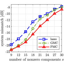
(a) SNR 20 dB

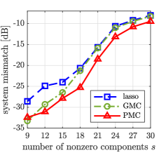
(b) SNR 30 dB

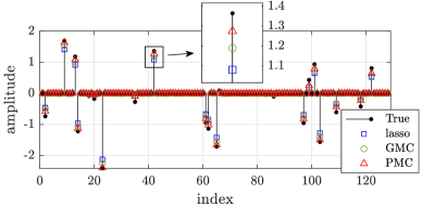
(c) average estimates for SNR $20$ dB ($s:=21$)

Figure 2: Experiment A: Learning curves and the average estimates.

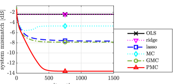
Figure 3: Experiment A: A particular instance in which a direct application of the MC penalty to an underdetermined system fails.

IV-B Experiment B: Robust regression in the presence of outlier

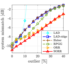
(a) SNR 10 dB, SOR $-30$ dB

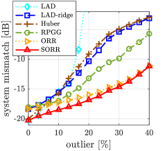
(b) SNR 20 dB, SOR $-40$ dB

Figure 4: Experiment B: System mismatch across outlier density.

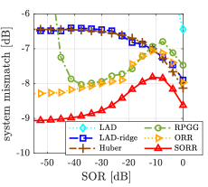
(a) SNR 10 dB, outlier 15 %

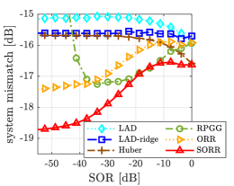
(b) SNR 20 dB, outlier 10 %

Figure 5: Experiment B: System mismatch across SOR.

We compare the performances of SORR and ORR (see Section II-B) for robust regression with those of LAD [5], LAD-ridge ($\ell_{1}$-loss $+$ Tikhonov regularization), Huber’s loss ${}^{\gamma}\left\|\cdot\right\|_{1}$ [2, 5], and the state-of-the-art method called the robust projected generalized gradient (RPGG) algorithm [35] which is based on the following formulation: $\min_{x\in\mathbb{R}^{n},e\in{\mathbb{R}}^{m}}\mu(\|\cdot\|_{1})_{\gamma_{1}^{-1}I}(x)+(\|\cdot\|_{1})_{\gamma_{2}^{-1}I}(e)$ subject to $y=Ax+e$ for $\gamma_{1},\gamma_{2}\in(0,+\infty]$. The sparse outlier model $y:=Ax_{\star}+\varepsilon_{\star}+o_{\diamond}$ is used, where the input matrix $A\in{\mathbb{R}}^{m\times n}$ and noise $\varepsilon_{\star}\in{\mathbb{R}}^{m}$ are generated randomly with $m:=128$ and $n:=64$ in the same way as in Experiment A. To show that SORR is stable under large Gaussian noise, we consider the cases of SNR 10 dB and 20 dB. The nonsparse vector $x_{\star}\in{\mathbb{R}}^{n}$ is generated randomly from the i.i.d. standard Gaussian distribution (i.e., $\sigma_{x_{\star}}^{2}:=1$). The outlier vector $o_{\diamond}$ is sparse with nonzero positions chosen randomly and with nonzero components generated from an i.i.d. zero-mean Gaussian distribution with variance determined by the signal-to-outlier ratio (SOR) $(\|Ax_{\star}\|_{2}^{2}/m)[\|o_{\diamond}\|_{2}^{2}/{\rm supp}(o_{\diamond})]^{-1}$. Here, ${\rm supp}(x):=\left|\{i\in\{1,2,\cdots,m\}\mid x_{i}\neq 0\}\right|$ is the support of a vector $x\in{\mathbb{R}}^{m}$. For SORR, $\sigma_{x}^{2}:=\sigma_{x_{\star}}^{2}$ and $\sigma_{\varepsilon}^{2}:=\sigma_{\varepsilon_{\star}}^{2}$ are used to show the potential performance. For the primal-dual debiasing algorithm, the parameters are chosen as follows. The parameters $\tau$ and $\sigma$ are set to slightly smaller values than the upper bounds, respectively, shown under Algorithm 1. We simply let $\beta_{k}:=1$ for all $k\in{\mathbb{N}}$, and tune $\gamma$ and $\mu$ based on Proposition 3 by grid search to attain the best performance. For RPGG, we let $\gamma_{1}:=+\infty$ (i.e., $(\|\cdot\|_{1})_{\gamma_{1}^{-1}I}=\left\|\cdot\right\|_{1}$) as $x_{\star}$ is nonsparse, and tune $\mu$ and $\gamma_{2}$ as well as the step size by grid search. For the other methods involving regularizers, the regularization parameters are tuned by grid search to attain the best performance. For Huber’s loss, $\gamma$ is chosen to attain the best performance. The results are averaged over 300 trials.

Figure 4 plots the results across outlier density ${\rm supp}(o_{\diamond})/m$. The proposed SORR method exhibits highly accurate and stable performances, and it outperforms all the other methods significantly. To be specific, the difference from ORR is notable when the outlier density is low to middle. It should be mentioned that LAD performed poorly due to the presence of heavy noise as well as strong outliers. Figure 5 plots the results across SOR to show the impacts of the change of the outlier power on the performance. Remarkably, the performances of SORR and ORR even improve as SOR decreases below $-12$ dB. This is because the influence of huge outliers on the MC loss vanishes above a certain range due to the same reason as for Tukey’s loss [5] and because such huge outliers will be easier to detect at the same time. The results clearly indicate the remarkable robustness of SORR (and ORR) against huge outliers. We mention that RPGG also exhibits a similar tendency over a reasonable range, although its performance degrades for SOR below $-40$ dB.

V Concluding Remarks

We presented the efficient framework based on the LiMES model. The PMC penalty composes the Moreau envelope contained in the standard MC penalty with the projection operator onto the input subspace, thereby restricting the Moreau-enhancement effect to the subspace for preserving the overall convexity even in the underdetermined case. SORR distinguishes Gaussian noise and sparse outlier explicitly to attain stable performances in highly noisy situations. The convexity conditions for those specific instances were discussed in a unified fashion with the LiMES model. While the LiMES function is “nonseparable”, the objective function involved in the Moreau envelope is “separable”. This mixed nature of separability and nonseparability allows an application of the LiMES model to the case when the fidelity term is not strongly convex (as in the underdetermined case of linear regression) with an efficient implementation using the proximal gradient method. The operators $\mathscr{L}$ and ${\mathscr{A}}_{2}$ play key roles in the model: $\mathscr{L}$ corresponds to the projection mentioned above and ${\mathscr{A}}_{2}$ takes care of robust regression. The proximal debiasing algorithms to compute the LiMES model require convexity of the smooth part of the objective function, for which a sufficient condition was presented. The condition was shown to be a necessary condition as well under the nonempty-interior assumption when the seed function is a support function. This is the case for instance when the seed function is a norm and the range of ${\mathscr{A}}_{2}$ contains the zero vector. Applications of the LiMES model to SPCP and robust classification were also presented. The hinge loss function widely used for robust classification was shown to be expressed as a composition of the support function of a closed interval $[-1,0]$ and an affine operator. Numerical examples showed that (i) the PMC penalty achieved debiased sparse modeling for underdetermined systems as well as outperforming GMC, and that (ii) SORR achieved stable and remarkably robust performances in the presence of both heavy Gaussian noise and sparse outlier as well as outperforming the existing robust methods including LAD, Huber’s loss, and RPGG.

The LiMES model will serve as a powerful tool to enhance performances with respect to a variety of penalty/loss functions based on the solid foundation of convex analysis, and there are plenty of opportunities to explore its further applications. In particular, it is our future works to investigate the efficacy of the LiMES model in SPCP and robust classification.

Appendix A Proof of Proposition 2

Since $c:=0$ for the debiased sparse modeling, the smooth part of (4) is convex if and only if ($\spadesuit$) is satisfied by Corollary 1. By definition of $\mathcal{M}:={\rm range}\hskip 1.99997ptA^{\top}$, moreover, it holds that $P_{\mathcal{M}}A^{\top}=A^{\top}$, from which together with $P_{\mathcal{M}}=P_{\mathcal{M}}\circ P_{\mathcal{M}}$ it follows that ($\spadesuit$) $\Leftrightarrow M_{1}^{\top}M_{1}-\mu M_{2}^{\top}\mathscr{L}^{\top}D^{2}\mathscr{L}M_{2}=A^{\top}A-\mu\gamma^{-1}P_{\mathcal{M}}=P_{\mathcal{M}}(A^{\top}A-\mu\gamma^{-1}I)P_{\mathcal{M}}\succeq O\Leftrightarrow\lambda_{\min}^{++}(A^{\top}A)\geq\mu\gamma^{-1}$. $\blacksquare$

Appendix B Proof of Proposition 3

According to the discussions in Section III-E, (8) is equivalent to (26). Since ${\rm range}\hskip 1.99997ptM_{2}={\rm range}\hskip 1.99997pt[A~{}I_{m}]={\mathcal{Z}}$ for SORR, the smooth part of (26) is convex if and only if ($\spadesuit$) is satisfied by Corollary 1. We prove the equivalence ($\spadesuit$) $\Leftrightarrow$ (10) below.

For $\Sigma_{\xi}^{-1}={\rm diag}(\sigma_{x}^{-2}I_{n},\sigma_{\varepsilon}^{-2}I_{m})$, it holds that ($\spadesuit$) $\Leftrightarrow M_{1}^{\top}M_{1}-\mu M_{2}^{\top}\mathscr{L}^{\top}D^{2}\mathscr{L}M_{2}=\Sigma_{\xi}^{-1}-\mu\gamma^{-1}[A~{}I_{m}]^{\top}[A~{}I_{m}]\succeq O$ which can be expressed equivalently as follows:

$$\left[\begin{array}[]{cc}\mu^{-1}\gamma\sigma_{x}^{-2}I_{n}-A^{\top}A&-A^{\top}\\ -A&(\mu^{-1}\gamma\sigma_{\varepsilon}^{-2}-1)I_{m}\\ \end{array}\right]\succeq O.$$ (B.1)

By [60, Theorem 7.7.9], (B.1) holds if and only if all of the following conditions are satisfied:

1. $\mu^{-1}\gamma\sigma_{x}^{-2}I_{n}-A^{\top}A\succeq O~{}(\Leftrightarrow\mu\lambda_{\max}(A^{\top}A)\leq\gamma\sigma_{x}^{-2})$;

2. $(\mu^{-1}\gamma\sigma_{\varepsilon}^{-2}-1)I_{m}\succeq O~{}(\Leftrightarrow\mu\leq\gamma\sigma_{\varepsilon}^{-2})$;

3. $-A^{\top}=(\mu^{-1}\gamma\sigma_{x}^{-2}I_{n}-A^{\top}A)^{1/2}\Upsilon((\mu^{-1}\gamma\sigma_{\varepsilon}^{-2}-1)I_{m})^{1/2}$ for some $\Upsilon\in{\mathbb{R}}^{n\times m}$ with its largest singular value at most one.

If $A=O$, then conditions (i) and (iii) hold trivially, and condition (ii) coincides with (10). Assume that $A\neq O$ in the following. We shall show below that (i)–(iii) $\Leftrightarrow$ (10). Suppose that conditions (i)–(iii) are satisfied. Condition (iii) under $A\neq O$ implies that $\mu^{-1}\gamma\sigma_{\varepsilon}^{-2}-1\neq 0$, and hence $\mu^{-1}\gamma\sigma_{\varepsilon}^{-2}-1>0$ by condition (ii). The equality in condition (iii) above can be rewritten as

$$\nu_{\varepsilon}A^{\top}=(\nu_{x}I_{n}-A^{\top}A)^{1/2}\tilde{\Upsilon},$$ (B.2)

where $\nu_{\varepsilon}:=(\mu^{-1}\gamma\sigma_{\varepsilon}^{-2}-1)^{-1/2}>0$, $\nu_{x}:=\mu^{-1}\gamma\sigma_{x}^{-2}>0$, and $\tilde{\Upsilon}:=-\Upsilon$. Let $A=V\Sigma U^{\top}$ be a singular value decomposition of $A$, where $U\in{\mathbb{R}}^{n\times n}$ and $V\in{\mathbb{R}}^{m\times m}$ are orthogonal matrices, and $\Sigma={\rm diag}(\varsigma_{1},\varsigma_{2},\cdots,\varsigma_{\min\{n,m\}})\in{\mathbb{R}}^{m\times n}$ having $\varsigma_{1}\geq\varsigma_{2}\geq\cdots\geq\varsigma_{\min\{n,m\}}\geq 0$ for the diagonal entries and zeros for the off-diagonal entries. Then, (B.2) can be rewritten as

$$U(\nu_{\varepsilon}\Sigma^{\top})V^{\top}= ~{}U(\nu_{x}I_{n}-\Sigma^{\top}\Sigma)^{1/2}U^{\top}\tilde{\Upsilon}$$

$$\Leftrightarrow\nu_{\varepsilon}\Sigma^{\top}= ~{}(\nu_{x}I_{n}-\Sigma^{\top}\Sigma)^{1/2}U^{\top}\tilde{\Upsilon}V.$$ (B.3)

Let $\tilde{\Upsilon}=-\Upsilon=U\Xi V^{\top}$ for some matrix $\Xi\in{\mathbb{R}}^{n\times m}$. Then, (B.3) reads

$$\nu_{\varepsilon}\Sigma^{\top}=(\nu_{x}I_{n}-\Sigma^{\top}\Sigma)^{1/2}\Xi.$$ (B.4)

Noting that $\varsigma_{1}>0$ due to the assumption $A\neq O$, one can verify from (B.4) that $\Xi$ must be written in the following form:

$$\Xi={\rm diag}(\varsigma_{1,\Upsilon},\Xi_{2,2})\in{\mathbb{R}}^{n\times m},$$ (B.5)

of which the $(1,1)$ entry is $\varsigma_{1,\Upsilon}>0$, the lower-right submatrix is $\Xi_{2,2}\in{\mathbb{R}}^{(n-1)\times(m-1)}$, and the entries of the off-diagonal blocks are zeros. By (B.4) and (B.5), we obtain

$$\nu_{\varepsilon}\varsigma_{1}=(\nu_{x}-\varsigma_{1}^{2})^{1/2}\varsigma_{1,\Upsilon},$$ (B.6)

where $\nu_{x}-\varsigma_{1}^{2}>0$ as $\nu_{\varepsilon}\varsigma_{1}>0$. To see that $\varsigma_{1,\Upsilon}$ is a singular value of $\Upsilon$ (or that of $\tilde{\Upsilon}$ equivalently), let $\Xi_{2,2}:=V_{\Xi_{2,2}}\Sigma_{\Xi_{2,2}}U_{\Xi_{2,2}}^{\top}$ be a singular value decomposition of $\Xi_{2,2}$, where $V_{\Xi_{2,2}}\in{\mathbb{R}}^{(n-1)\times(n-1)}$ and $U_{\Xi_{2,2}}^{\top}\in{\mathbb{R}}^{(m-1)\times(m-1)}$ are orthogonal matrices, and $\Sigma_{\Xi_{2,2}}:={\rm diag}(\varsigma_{2,\Upsilon},\varsigma_{3,\Upsilon},\cdots,\varsigma_{\min\{n,m\},\Upsilon})\in{\mathbb{R}}^{(n-1)\times(m-1)}$ for singular values $\varsigma_{i,\Upsilon}\geq 0$ for $i\in\{2,3,\cdots,\min\{n,m\}\}$. It then follows that $\Xi=V_{\Xi}\Sigma_{\Xi}U_{\Xi}^{\top}$, where $V_{\Xi}:={\rm diag}(1,V_{\Xi_{2,2}})$, $U_{\Xi}:={\rm diag}(1,U_{\Xi_{2,2}})$, and $\Sigma_{\Xi}:={\rm diag}(\varsigma_{1,\Upsilon},\Sigma_{\Xi_{2,2}})$. Thus, $\Upsilon=U_{\Upsilon}\Sigma_{\Upsilon}V_{\Upsilon}^{\top}$ gives a singular value decomposition of $\Upsilon$ with $U_{\Upsilon}:=-UU_{\Xi}$, $\Sigma_{\Upsilon}:=\Sigma_{\Xi}$, and $V_{\Upsilon}:=VV_{\Xi}$, where $U_{\Upsilon}$ and $V_{\Upsilon}$ are clearly orthogonal matrices. Therefore, $\varsigma_{1,\Upsilon}$ is a singular value of $\Upsilon$, and thus (B.6) and condition (iii) imply that

$$~{}\varsigma_{1,\Upsilon}^{2}=\frac{\nu_{\varepsilon}^{2}\varsigma_{1}^{2}}{\nu_{x}-\varsigma_{1}^{2}}\leq 1$$ (B.7a)

$$\Leftrightarrow ~{}\varsigma_{1}^{2}\leq(\mu^{-1}\gamma\sigma_{\varepsilon}^{-2}-1)(\mu^{-1}\gamma\sigma_{x}^{-2}-\varsigma_{1}^{2}).$$ (B.7b)

After a simple manipulation of (B.7b) under conditions (i) and (ii) with $\varsigma_{1}^{2}=\lambda_{\max}(A^{\top}A)$, we obtain (10).

Conversely, suppose that (10) holds. Then, conditions (i) and (ii) hold immediately, and it is therefore sufficient to inspect condition (iii). It is clear that (10) implies the inequality in (B.7a). Since $\nu_{\varepsilon}^{2}\varsigma^{2}/(\nu_{x}-\varsigma^{2})$ is an increasing function of $\varsigma^{2}\in[0,\nu_{x})$, (B.7a) implies that

$$\varsigma_{i,\Upsilon}:=\frac{\nu_{\varepsilon}\varsigma_{i}}{(\nu_{x}-\varsigma_{i}^{2})^{1/2}}\in(0,1],~{}\forall\varsigma_{i}>0.$$ (B.8)

Let $\varsigma_{i,\Upsilon}:=0$ for all $\varsigma_{i}=0$ if any. Define a diagonal matrix $\Sigma_{\Upsilon}\in{\mathbb{R}}^{n\times m}$, in the same way as above, with diagonal entries $\varsigma_{i,\Upsilon}$. Redefine the matrices $\Upsilon:=V\Sigma_{\Upsilon}(-U)^{\top}$ and $\tilde{\Upsilon}:=V\Sigma_{\Upsilon}U^{\top}$. Then, $\Upsilon$ and $\tilde{\Upsilon}$ have the singular values $\varsigma_{i,\Upsilon}\in[0,1]$, $i\in\{1,2,\cdots,\min\{n,m\}\}$. Since $\tilde{\Upsilon}$ satisfies $\eqref{eq:condition3b}$ and thus $\eqref{eq:condition3a}$, $\Upsilon$ satisfies the equation of condition (iii). $\blacksquare$

Appendix C Proof of Lemma 3

Let $\mathcal{V}^{\perp}\subset{\mathcal{X}}$ denote the orthogonal complement of $\mathcal{V}$. Then, it follows that

$${}^{\gamma}(\psi\circ\mathfrak{A})(x)= ~{}\min_{u\in{\mathcal{X}}}~{}\big{[}\psi(\mathfrak{A}u)+0.5\gamma^{-1}\left\|u-x\right\|^{2}\big{]}$$

$$= ~{}\min_{u\in{\mathcal{X}}}~{}\big{[}\psi(\mathfrak{L}u+b)+0.5\gamma^{-1}(\left\|P_{\mathcal{V}}u-P_{\mathcal{V}}x\right\|^{2}$$

$$\hskip 28.00006pt+\left\|P_{\mathcal{V}^{\perp}}u-P_{\mathcal{V}^{\perp}}x\right\|^{2})\big{]}$$

$$= ~{}\min_{u\in{\mathcal{X}}}~{}\big{[}\psi(\mathfrak{L}u+b)+0.5\gamma^{-1}\left\|P_{\mathcal{V}}u-P_{\mathcal{V}}x\right\|^{2}\big{]}$$

$$= ~{}\min_{u\in{\mathcal{X}}}~{}\big{[}\psi(\mathfrak{L}u+b)+0.5\gamma^{-1}\left\|\mathfrak{L}u-\mathfrak{L}x\right\|^{2}\big{]}$$

$$= ~{}\min_{z\in{\mathcal{K}}}~{}\big{[}\psi(z+b)+0.5\gamma^{-1}\left\|z-\mathfrak{L}x\right\|^{2}\big{]}$$

$$= ~{}\min_{v\in{\mathcal{K}}}~{}\big{[}\psi(v)+0.5\gamma^{-1}\left\|v-\mathfrak{A}x\right\|^{2}\big{]}$$

$$= ~{}^{\gamma}\psi(\mathfrak{A}x).$$ (C.1)

Here, the second equality is due to the Pythagorean theorem, the third equality holds because $\psi(\mathfrak{L}u+b)$ is independent of $P_{\mathcal{V}^{\perp}}u$, the fourth equality is due to $\mathfrak{L}^{*}\mathfrak{L}=P_{\mathcal{V}}=P_{\mathcal{V}}^{*}\circ P_{\mathcal{V}}$, and finally the fifth equality is due to ${\rm range}\hskip 1.99997pt\mathfrak{L}={\mathcal{K}}$. By (C.1), it follows that $(\psi\circ\mathfrak{A})_{\gamma^{-1/2}I}(x)=\psi(\mathfrak{A}x)-~{}^{\gamma}(\psi\circ\mathfrak{A})(x)=(\psi-\hskip 1.00006pt^{\gamma}\psi)(\mathfrak{A}x)$, which completes the proof. $\blacksquare$

Masahiro Yukawa received the B.E., M.E., and Ph.D. degrees from the Tokyo Institute of Technology in 2002, 2004, and 2006, respectively. He is a Professor with the Department of Electronics and Electrical Engineering, Keio University, Yokohama, Japan. He is currently a Senior Area Editor of the IEEE Transactions on Signal Processing. He served as an Associate Editor for the IEEE Transactions on Signal Processing from 2015 to 2019, the Springer Journal of Multidimensional Systems and Signal Processing from 2012 to 2016, and the IEICE Transactions on Fundamentals of Electronics, Communications and Computer Sciences from 2009 to 2013. His research interests include mathematical adaptive signal processing, convex/sparse optimization, and machine learning. Dr. Yukawa received the JSPS Prize in 2021, the Young Scientists’ Prize, the Commendation for Science and Technology by the Minister of Education, Culture, Sports, Science and Technology in 2014, the Excellent Paper Award from the IEICE in 2006, among many others. He is a Member of the IEICE.

Hiroyuki Kaneko received the B.E. and M.E. degrees in Electronics and Electrical Engineering from Keio University, Yokohama, Japan, in 2020 and 2022, respectively. He is currently a Researcher with NTT Communication Science Laboratories, NTT Corporation, Kyoto, Japan. His research interests include sparse signal processing, convex optimization, and audio signal processing.

Kyohei Suzuki (Student Member, IEEE) received the B.E. and M.E. degrees in Electronics and Electrical Engineering from Keio University, Yokohama, Japan, in 2020 and 2022, respectively. He is currently working toward the Ph.D. degree in Electronics and Electrical Engineering from Keio University, Yokohama, Japan. His research interests include mathematical signal processing, sparse optimization, and robust statistics.

Isao Yamada received the B.E. degree in computer science from the University of Tsukuba, Tsukuba, Japan, in 1985, and the M.E. and Ph.D. degrees in electrical and electronic engineering from the Tokyo Institute of Technology, Tokyo, Japan, in 1987 and 1990, respectively. He is currently a Professor with the Department of Information and Communications Engineering, Tokyo Institute of Technology. His current research interests are in mathematical signal processing, nonlinear inverse problems, and optimization theory. He has been the IEICE Fellow since 2015. He was the recipient of the MEXT Minister Award (Research Category), the IEEE Signal Processing Magazine Best Paper Award in 2015, the IEICE Excellent Paper Awards (in 1991, 1995, 2006, 2009, 2014 and 2022), the IEICE Achievement Award in 2009, the ICF Research Award in 2004, the Docomo Mobile Science Award (Fundamental Science Division) in 2005 and the Fujino Prize in 2008. He served as a member of the IEEE Signal Processing Society Awards Board in 2022.

References

- [1] S. Theodoridis, Machine Learning: A Bayesian and Optimization Perspective, 2nd ed. London: Academic Press, 2020.
- [2] A. M. Zoubir, V. Koivunen, E. Ollila, and M. Muma, Robust Statistics for Signal Processing. Cambridge: Cambridge University Press, 2018.
- [3] M. Elad, Sparse and Redundant Representations: From Theory to Applications in Signal and Image Processing. New York: Springer, 2010.
- [4] S. Foucart and H. Rauhut, A Mathematical Introduction to Compressive Sensing. New York: Springer, 2013.
- [5] P. J. Huber and E. M. Ronchetti, Robust Statistics, 2nd ed. Wiley, 2009.
- [6] S. Pesme and N. Flammarion, “Online robust regression via SGD on the loss,” in Advances in Neural Information Processing Systems, vol. 33, 2020, pp. 2540–2552.
- [7] R. Chartrand and V. Staneva, “Restricted isometry properties and nonconvex compressive sensing,” Inverse Problems, vol. 24, no. 3, pp. 1–14, 2008.
- [8] G. Marjanovic and V. Solo, “On optimization and matrix completion,” IEEE Trans. Signal Process., vol. 60, no. 11, pp. 5714–5724, Nov. 2012.
- [9] X. Shen and Y. Gu, “Nonconvex sparse logistic regression with weakly convex regularization,” IEEE Trans. Signal Process., vol. 66, no. 12, pp. 3199–3211, June 2018.
- [10] Q. Yao and J. T. Kwok, “Efficient learning with a family of nonconvex regularizers by redistributing nonconvexity,” J. Machine Learn. Research, vol. 18, no. 179, pp. 1–52, 2018.
- [11] B. Wen, X. Chen, and T. K. Pong, “A proximal difference–of–convex algorithm with extrapolation,” Comput. Optim. Appl., vol. 69, no. 2, pp. 297–324, Oct. 2018.
- [12] R. Chartrand, “Exact reconstruction of sparse signals via nonconvex minimization,” IEEE Signal Process. Lett., vol. 14, no. 10, pp. 707–710, Oct. 2007.
- [13] M. Yukawa and S. Amari, “-regularized least squares () and critical path,” IEEE Trans. Information Theory, vol. 62, no. 1, pp. 488–502, Jan. 2016.
- [14] K. Jeong, M. Yukawa, and S. Amari, “Can critical-point paths under -regularization () reach the sparsest least squares solutions?” IEEE Trans. Information Theory, vol. 60, no. 5, pp. 2960–2968, May 2014.
- [15] T. Zhang, “Some sharp performance bounds for least squares regression with regularization,” The Annals of Statistics, vol. 37, no. 5A, pp. 2109–2144, Oct. 2009.
- [16] E. J. Candes, M. B. Wakin, and S. P. Boyd, “Enhancing sparsity by reweighted minimization,” J. Fourier Analysis and Applications, vol. 14, no. 5–6, pp. 877–905, Oct. 2008.
- [17] C. H. Zhang, “Nearly unbiased variable selection under minimax concave penalty,” The Annals of Statistics, vol. 38, no. 2, pp. 894–942, Apr. 2010.
- [18] J. Fan and R. Li, “Variable selection via nonconcave penalized likelihood and its oracle properties,” J. American Statistical Association, vol. 96, no. 456, pp. 1348–1360, Dec. 2001.
- [19] E. Soubies, L. Blanc-Féraud, and A. G., “A continuous exact penalty (CEL0) for least squares regularized problem,” SIAM J. Imaging Sci., vol. 8, no. 3, pp. 1607–1639, 2015.
- [20] F. Wen, L. Chu, P. Liu, and R. Qiu, “A survey on nonconvex regularization based sparse and low-rank recovery in signal processing, statistics, and machine learning,” IEEE Access, vol. 6, pp. 69 883–69 906, Nov. 2018.
- [21] A. Blake and A. Zisserman, Visual Reconstruction. Cambridge, MA: MIT Press, 1987.
- [22] M. Nikolova, “Markovian reconstruction using a GNC approach,” IEEE Trans. Image Process., vol. 8, no. 9, pp. 1204–1220, Sep. 1999.
- [23] T. P. Dinh and E. B. Souad, Algorithms for solving a class of nonconvex optimization problems: Methods of subgradient, ser. Fermat Days 85: Mathematics for Optimization. Elsevier, 1986, vol. 129, pp. 249–271.
- [24] A. Parekh and I. W. Selesnick, “Enhanced low-rank matrix approximation,” IEEE Signal Process. Lett., vol. 23, no. 4, pp. 493–497, Apr. 2016.
- [25] A. Lanza, S. Morigi, I. W. Selesnick, and F. Sgallari, “Sparsity-inducing nonconvex nonseparable regularization for convex image processing,” SIAM J. Imaging Sci., vol. 12, no. 2, pp. 1099–1134, 2019.
- [26] J. Abe, M. Yamagishi, and I. Yamada, “Linearly involved generalized Moreau enhanced models and their proximal splitting algorithm under overall convexity condition,” Inverse Problems, vol. 36, no. 3, pp. 1–36, Feb. 2020.
- [27] I. Selesnick, “Sparse regularization via convex analysis,” IEEE Trans. Signal Process., vol. 65, no. 17, pp. 4481–4494, Sep. 2017.
- [28] J. Abe, M. Yamagishi, and I. Yamada, “Convexity-edge-preserving signal recovery with linearly involved generalized minimax concave penalty function,” in Proc. IEEE ICASSP, 2019, pp. 4918–4922.
- [29] M. Yan, “Restoration of images corrupted by impulse noise and mixed Gaussian impulse noise using blind inpainting,” SIAM J. Imag. Sci., vol. 6, no. 3, pp. 1227–1245, July 2013.
- [30] K. Hohm, M. Storath, and A. Weinmann, “An algorithmic framework for Mumford-Shah regularization of inverse problems in imaging,” Inverse Problem, vol. 31, no. 11, pp. 1–30, 2015.
- [31] G. Yuan and B. Ghanem, “L0 TV: A new method for image restoration in the presence of impulse noise,” in Proc. IEEE Conf. Comput. Vis. Pattern Recognit., 2015, pp. 5369–5377.
- [32] F. Wen, L. Adhikari, L. Pei, R. F. Marcia, P. Liu, and R. C. Qiu, “Nonconvex regularization based sparse recovery and demixing with application to color image inpainting,” IEEE Access, vol. 5, pp. 11 513–11 527, May 2017.
- [33] A. Javaheri, H. Zayyani, M. A. T. Figueiredo, and F. Marvasti, “Robust sparse recovery in impulsive noise via continuous mixed norm,” IEEE Signal Process. Lett., vol. 25, no. 8, pp. 1146–1150, Aug. 2018.
- [34] G. Tzagkarakis, J. P. Nolan, and P. Tsakalides, “Compressive sensing using symmetric alpha-stable distributions for robust sparse signal reconstruction,” IEEE Trans. Signal Process., vol. 67, no. 3, pp. 808–820, Feb. 2019.
- [35] C. Yang, X. Shen, H. Ma, B. Chen, Y. Gu, and H. C. So, “Weakly convex regularized robust sparse recovery methods with theoretical guarantees,” IEEE Trans. Signal Process., vol. 67, no. 19, pp. 5046–5061, Oct. 2019.
- [36] Z. Zhou, X. Li, J. Wright, E. Candes, and Y. Ma, “Stable principal component pursuit,” in Proc. IEEE Int. Symp. Inf. Theory, 2010, p. 1518–1522.
- [37] M. Yukawa, K. Suzuki, and I. Yamada, “Stable robust regression under sparse outlier and gaussian noise,” in Proc. EUSIPCO, 2022, pp. 2236–2240.
- [38] J. J. Moreau, “Fonctions convexes duales et points proximaux dans un espace hilbertien,” C. R. Acad. Sci. Paris Ser. A Math., vol. 255, pp. 2897–2899, 1962.
- [39] ——, “Proximité et dualité dans un espace hilbertien,” Bull. Soc. Math. France, vol. 93, pp. 273–299, 1965.
- [40] P. L. Combettes and V. R. Wajs, “Signal recovery by proximal forward-backward splitting,” SIAM Journal on Multiscale Modeling and Simulation, vol. 4, no. 4, pp. 1168–1200, 2005.
- [41] I. Yamada, M. Yukawa, and M. Yamagishi, Fixed-Point Algorithms for Inverse Problems in Science and Engineering, ser. Optimization and Its Applications. New York: Springer, 2011, vol. 49, ch. 17, pp. 345–390.
- [42] H. H. Bauschke and P. L. Combettes, Convex Analysis And Monotone Operator Theory in Hilbert Spaces, 2nd ed. New York: NY: Springer, 2017.
- [43] A. Javanmard and A. Montanari, “Confidence intervals and hypothesis testing for high-dimensional regression,” J. Machine Learning Research, vol. 15, pp. 2869–2909, 2014.
- [44] I. W. Selesnick and I. Bayram, “Enhanced sparsity by non-separable regularization,” IEEE Trans. Signal Process., vol. 64, no. 9, pp. 2298–2313, 2016.
- [45] P. L. Lions and B. Mercier, “Splitting algorithms for the sum of two nonlinear operators,” SIAM J. Numer. Anal., vol. 16, no. 6, pp. 964–979, 1979.
- [46] P. L. Combettes and V. R. Wajs, “Signal recovery by proximal forward-backward splitting,” Multiscale Model. Simul., vol. 4, no. 4, pp. 1168–1200, 2005.
- [47] A. Beck and M. Teboulle, “A fast iterative shrinkage-thresholding algorithm for linear inverse problems,” SIAM J. Imaging Sciences, vol. 2, no. 1, pp. 183–202, 2009.
- [48] H. Kaneko and M. Yukawa, “Normalized least-mean-square algorithms with minimax concave penalty,” in Proc. IEEE ICASSP, 2020, pp. 5440–5444.
- [49] E. J. Candes and P. A. Randall, “Highly robust error correction by convex programming,” IEEE Trans. Inform. Theory, vol. 54, no. 7, pp. 2829–2840, 2008.
- [50] F. R. Hampel, E. M. Ronchetti, P. J. Rousseeuw, and W. A. Stahel, Robust statistics: the approach based on influence functions. John Wiley & Sons, 2011, vol. 196.
- [51] A. E. Beaton and J. W. Tukey, “The fitting of power series, meaning polynomials, illustrated on band-spectroscopic data,” Technometrics, vol. 16, no. 2, pp. 147–185, May 1974.
- [52] I. Selesnick and M. Farshchian, “Sparse signal approximation via nonseparable regularization,” IEEE Trans. Signal Process., vol. 65, no. 10, pp. 2561–2575, 2017.
- [53] K. Suzuki and M. Yukawa, “Robust recovery of jointly-sparse signals using minimax concave loss function,” IEEE Trans. Signal Process., vol. 69, pp. 669–681, 2021.
- [54] ——, “Sparse stable outlier-robust signal recovery under Gaussian noise,” IEEE Trans. Signal Process., 2023, accepted for publication.
- [55] T. Koyakumaru, M. Yukawa, E. Pavez, and A. Ortega, “A graph learning algorithm based on Gaussian Markov random fields and minimax concave penalty,” in Proc. IEEE ICASSP, 2021, pp. 5390–5394.
- [56] ——, “Learning sparse graph with minimax concave penalty under Gaussian Markov random fields,” IEICE Trans. Fundamentals, vol. E106-A, no. 1, pp. 23–34, Jan. 2023.
- [57] K. Komuro, M. Yukawa, and R. L. G. Cavalcante, “Distributed sparse optimization with weakly convex regularizer: Consensus promoting and approximate Moreau enhanced penalties towards global optimality,” IEEE Trans. Signal and Inform. Process. over Netw., vol. 8, pp. 514–527, 2022.
- [58] S. Mallat, A Wavelet Tour of Signal Processing: The Sparse Way, 3rd ed. Academic Press, 2009.
- [59] H. Du and Y. Liu, “Minmax-concave total variation denoising,” Signal, Image and Video Processing, vol. 12, pp. 1027–1034, 2018.
- [60] R. A. Horn and C. R. Johnson, Matrix Analysis, 2nd ed. New York: Cambridge University Press, 2013.
- [61] S. Boyd and L.Vandenberghe, Convex Optimization. Cambridge: Cambridge University Press, 2004.
- [62] E. Kreyszig, Introductory Functional Analysis with Applications. U.S.A.: Wiley, 1978.
- [63] I. Loris and C. Verhoeven, “On a generalization of the iterative soft-thresholding algorithm for the case of non-separable penalty,” Inverse Problems, vol. 27, no. 12, p. 125007 (15pp), 2011.
- [64] P. Chen, J. Huang, and X. Zhang, “A primal–dual fixed point algorithm for convex separable minimization with applications to image restoration,” Inverse Problems, vol. 29, no. 2, p. 025011 (33pp), 2013.
- [65] N. Komodakis and J.-C. Pesquet, “Playing with duality: An overview of recent primal–dual approaches for solving large-scale optimization problems,” IEEE Signal Processing Magazine, vol. 32, no. 6, pp. 31–54, Nov. 2015.
- [66] A. Chambolle and T. Pock, “A first-order primal-dual algorithm for convex problems with applications to imaging,” Journal of Mathematical Imaging and Vision, vol. 40, pp. 120–145, 2011.
- [67] L. Condat, “A primal dual splitting method for convex optimization involving Lipschitzian, proximable and linear composite terms,” J. Optim. Theory Appl., vol. 158, pp. 460–479, 2013.
- [68] L. Yin, A. Parekh, and I. Selesnick, “Stable principal component pursuit via convex analysis,” IEEE Trans. Signal Process., vol. 67, no. 10, pp. 2595–2607, May 2019.
- [69] M. O. Ulfarsson, V. Solo, and G. Marjanovic, “Sparse and low rank decomposition using penalty,” in Proc. IEEE ICASSP, 2015, pp. 3312–3316.
- [70] P. O. Hoyer, “Non-negative matrix factorization with sparseness constraints,” J. Machine Learn. Research, vol. 5, pp. 1457–1469, 2004.