Orders of magnitude reduction in the computational overhead for quantum many-body problems on quantum computers via an exact transcorrelated method

Abstract

Transcorrelated methods provide an efficient way of partially transferring the description of electronic correlations from the ground state wavefunction directly into the underlying Hamiltonian. In particular, Dobrautz et al. [Phys. Rev. B, 99(7), 075119, (2019)] have demonstrated that the use of momentum-space representation, combined with a non-unitary similarity transformation, results in a Hubbard Hamiltonian that possesses a significantly more “compact” ground state wavefunction, dominated by a single Slater determinant. This compactness/single-reference character greatly facilitates electronic structure calculations. As a consequence, however, the Hamiltonian becomes non-Hermitian, posing problems for quantum algorithms based on the variational principle. We overcome these limitations with the ansatz-based quantum imaginary time evolution algorithm and apply the transcorrelated method in the context of digital quantum computing. We demonstrate that this approach enables up to 4 orders of magnitude more accurate and compact solutions in various instances of the Hubbard model at intermediate interaction strength ($U/t=4$), enabling the use of shallower quantum circuits for wavefunction ansatzes. In addition, we propose a more efficient implementation of the quantum imaginary time evolution algorithm in quantum circuits that is tailored to non-Hermitian problems. To validate our approach, we perform hardware experiments on the ibmq_lima quantum computer. Our work paves the way for the use of exact transcorrelated methods for the simulations of ab initio systems on quantum computers.

I Introduction

Understanding and predicting the properties of materials and chemical systems is of paramount importance for the development of natural sciences and technology. To achieve this goal, classical computers are used to solve – at least approximately – the corresponding quantum mechanical equations and extract the quantities of interest. However, performing this type of calculation is a notoriously hard problem since the dimension of the many-body wavefunction scales exponentially with the number of degrees of freedom (e.g. number of electrons) Feynman (1982). This poses an important limitation on the size of accurately simulatable physical systems and makes the majority of them inaccessible on classical computers.

Quantum computing, on the other hand, is emerging as a new computational paradigm for the solution of many classically hard problems, including the solution of the many-body Schrödinger equation of strongly correlated systems. Nowadays, quantum computers are at the forefront of scientific research thanks to groundbreaking hardware demonstrations including (real-time) error mitigation Kandala et al. (2019) and error correction schemes Egan et al. (2021), paving the way for large near-term quantum calculations on noisy quantum hardware (with physical qubits), followed – in the near future – by fault-tolerant calculations with logical qubits Campbell et al. (2017); IBM (2021). From an algorithmic perspective, quantum computers can provide scaling advantages in the computation of the ground state and excited state properties (of isolated and periodic systems) Moll et al. (2018); Cao et al. (2019); McArdle et al. (2020); Liu et al. (2020); Yamamoto et al. (2021), vibrational structure calculations McArdle et al. (2019a); Sawaya et al. (2020); Ollitrault et al. (2020), configuration space sampling (such as protein folding) Rubiera et al. (2021); Robert et al. (2021), molecular and quantum dynamics Sokolov et al. (2021); Fedorov et al. (2021); Ollitrault et al. (2021) and lattice gauge theory Mathis et al. (2020); Mazzola et al. (2021), just to mention a few.

The currently most popular quantum optimization algorithm for electronic structure calculations is the variational quantum eigensolver (VQE) Peruzzo et al. (2014); McClean et al. (2016); Cao et al. (2019); Bauer et al. (2020); McArdle et al. (2020). It is a well-tested and well-developed hybrid quantum-classical approach: Quantum hardware is used to efficiently represent an arbitrary wavefunction ansatz $\ket{\Psi(\boldsymbol{\theta})}$, and measure the expectation value of a chosen observable $\bra{\Psi(\boldsymbol{\theta})}\hat{O}\ket{\Psi(\boldsymbol{\theta})}$, in conjunction with a classical computer which performs the optimization of the (quantum gate) parameters $\boldsymbol{\theta}$ until a chosen cost function of the observable $\hat{O}$ (e.g., the energy in electronic structure calculations) is minimized. However, most importantly for the scope of this work, the VQE algorithm is applicable only in the case where the cost function that drives the optimization of the parameters is Hermitian.

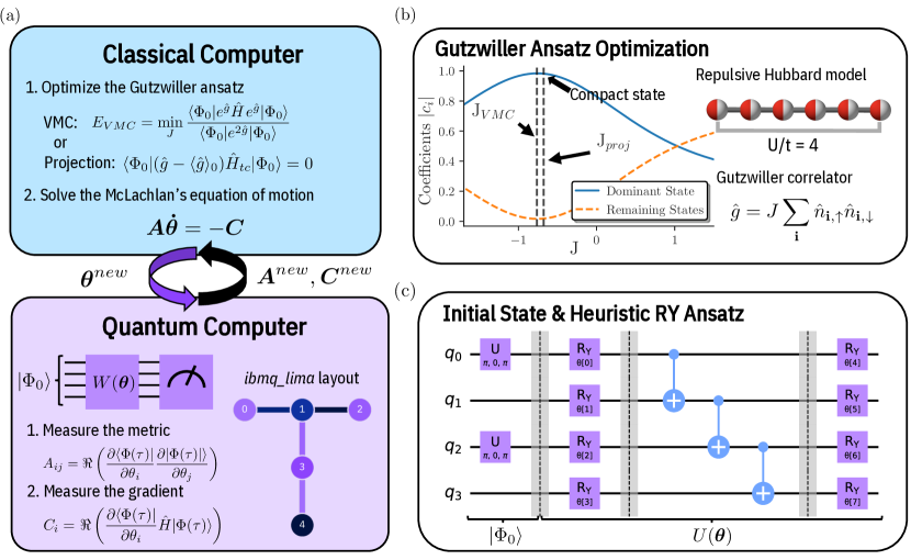
Figure 1: (a) Hybrid quantum-classical procedure employed to perform QITE. First, the Gutzwiller ansatz is optimized by VMC or projection on a classical computer. The resulting TC Hubbard Hamiltonian is represented as a sum of Pauli strings by a fermion-to-qubit mapping (e.g., Jordan-Wigner). The initial parameter values $\boldsymbol{\theta}$ and the list of necessary Pauli-string measurements are sent to the quantum computer. Given a wavefunction ansatz, $\ket{\Phi(\boldsymbol{\theta})}=U(\boldsymbol{\theta})\ket{\Phi_{0}}$, the matrix elements of the metric $A^{new}_{ij}$ and the gradient $C^{new}_{i}$ are measured using the differentiation of general gates via a linear combination of unitaries represented as $W(\boldsymbol{\theta})$ Schuld et al. (2019). Finally, the linear system derived from McLachlan’s variational principle is solved and by applying the Euler method, we obtain the parameters $\boldsymbol{\theta}^{new}$ of the next time-step. The whole procedure is repeated until convergence (i.e., Euclidean norm of the gradient is below a set threshold). (b) Optimization of the Jastrow parameter $J$. We show that when $J\approx J_{proj}$ or $J\approx J_{VMC}$, the ground state of 6-site TC momentum-space Hubbard model is “compact”, meaning almost the entire weight of the wavefunction is concentrated in the Hartree-Fock (HF) state. $J_{VMC}$ and $J_{proj}$ denote the results of a VMC simulation and the solution of the projective scheme, respectively. (c) Heuristic RY unitary operator ${U}(\boldsymbol{\theta})$ applied on the HF initial state $\ket{\Psi_{0}}$ of the 2-site Hubbard model. In purple are the single-qubit rotations and in blue are the CNOTs. The definitions of the single-qubit gates are given in Appendix A. Exactly this ansatz and initial state are employed in the hardware experiments on the imbq_lima chip (see its layout in panel (a) where numbers denote the qubits).

As an alternative to VQE, imaginary time evolution Motta et al. (2019) can be used to drive an initial wavefunction guess towards the optimal ground state solution. In particular, the ansatz-based quantum imaginary time evolution (QITE) algorithm is a powerful method for the calculation of the ground state of quantum systems by simulating the non-unitary dynamics on quantum computers McArdle et al. (2019b). Using the McLachlan variational principle McLachlan (1964) it is possible to describe time-evolution by means of a fixed-length variational circuit, whose parameters evolve according to a well-defined equation of motion which is solved classically. For a detailed analysis of this approach we refer to the original literature Yuan et al. (2019). Applications of the QITE algorithm include, for instance, the determination of ground and excited states Jones et al. (2019); Motta et al. (2019), the training of quantum machine learning models Zoufal et al. (2021a), the simulation of quantum field theories Liu and Xin (2020), the solution of linear systems of equations Huang et al. (2019); Xu et al. (2021) and combinatorial optimization problems Amaro et al. (2021), and the pricing of financial options Fontanela et al. (2021). Recent algorithmic developments include the addition of adaptive ansatzes Gomes et al. (2021), hardware-efficient approaches Benedetti et al. (2021) and derivation of robust error bounds Zoufal et al. (2021b).

Both the VQE and QITE approaches require sufficiently expressive ansatzes for the representation of the targeted ground state wavefunction Aspuru-Guzik et al. (2005); Babbush et al. (2018); Moll et al. (2018); McArdle et al. (2019b); Yuan et al. (2019), which would need exponentially many parameters for an exact solution. However, it was shown that a polynomial number of variational parameters (single-qubit rotations) is sufficient to achieve accurate results within a given error threshold Kitaev (1997); Woitzik et al. (2020). In this framework, we can therefore aim at solving interesting electronic structure problems using state-of-the-art noisy quantum devices (with limited coherence times and uncorrected gate operations) with relatively shallow circuits.

Despite these advancements, one of the major limitations of the application of current quantum algorithms to model systems, like the Hubbard model and the electronic structure problem, is the severely limited number of qubits. Every single-particle orbital used to describe a problem at hand needs a physical qubit to represent a system on quantum hardware. In the field of quantum chemistry, this is amplified by the need for large basis set expansion (and consequently qubits) to capture dynamic correlation effects induced by the divergence of the Coulomb potential and, therefore, to deal with the non-differentiable behavior of the electronic wavefunction at electron coalescence, known as Kato’s cusp condition Kato (1957); Pack and Brown (1966). As a consequence, various theories and approaches Hylleraas (1929); Szalewicz and Jeziorski (2010); Szalewicz et al. (1982); Mitroy et al. (2013); Szalewicz and Jeziorski (2010); Szalewicz et al. (1982); Mitroy et al. (2013) that aim to explicitly capture these dynamic correlation effects and obtain more accurate results in smaller basis sets exist in the field of computational chemistry; the most notable being the explicitly correlated R12 and F12 methods Kutzelnigg (1985); Kutzelnigg and Klopper (1991); Noga and Kutzelnigg (1994); Ten-no (2004a, b); Valeev (2004); Werner et al. (2007); Grüneis et al. (2017); Hättig et al. (2011); Kong et al. (2011); Ten-no (2012); Ten-no and Noga (2011). It is a very active field of research to exploit similar approaches in the field of quantum computing to reduce the quantum resources necessary to obtain accurate results for realistic systems on near-term quantum devices Takeshita et al. (2020); Kottmann et al. (2021); Schleich et al. (2021); Mazzola et al. (2019); Benfenati et al. (2021).

In this work we use the so-called transcorrelated (TC) method, introduced by Hirschfelder Hirschfelder (1963) and Boys and Handy Boys and Handy (1969a, b, c), and apply it to a lattice Hamiltonian in the form of the Hubbard model. The TC method was originally conceived in the field of ab initio quantum chemistry to exactly incorporate electronic correlation effects, via a correlated Jastrow ansatz Jastrow (1955) for the wavefunction, directly into the Hamiltonian by a similarity transformation (ST). However, the same basic concept can be applied to any problem, thus facilitating the subsequent solution. In the case of the Hubbard model in conjunction with a Gutzwiller correlator Gutzwiller (1963); Brinkman and Rice (1970), the ST introduces higher order interaction terms and renders the Hamiltonian non-Hermitian, but in a complete basis does not change its spectrum. As a consequence, the variational principle does not apply anymore, and we have to rely on methods like QITE to solve the problem on a quantum computer. (Another possible approach is to use VQE based on the variance cost function Zhang et al. (2020); Tsuneyuki (2008), but this would require to square the Hamiltonian and hence presents a significant overhead in terms of measurements (75).)

Following the approach of Dobrautz et al. Dobrautz et al. (2019a), McArdle and Tew McArdle and Tew (2020) recently investigated the exact non-Hermitian TC formulation of the Hubbard Hamiltonian in the real-space representation in the context of quantum computing. They investigated the beneficial effect of the TC approach on the quantum footprint that is caused by a more compact/single-reference right eigenvector. The advantages were demonstrated in numerical simulations using the QITE algorithm, however, without the complete implementation of the corresponding quantum circuits. Additionally, McArdle and Tew used the TC approach in the real-space representation of the Hubbard model, which, however, does not display the same level of compactification of the ground state wavefunction as in a momentum-space representationDobrautz et al. (2019a).

In this work, we expand and complement the study of McArdle and Tew McArdle and Tew (2020) by implementing the full algorithm as would be executed on a quantum computer. To validate our approach, we perform experiments on the IBM quantum computer, ibmq_lima. In addition, following Dobrautz et al. Dobrautz et al. (2019a), we investigate the formulation of the TC Hubbard Hamiltonian in the momentum space, for which we expect an increased efficiency of our method (compared to real space) while approaching the complexity of ab initio chemical problems (i.e., the presence of a 3-body term). Thus, this study on the TC Hubbard model in the momentum space will pave the way for future extensions to more general ab initio Hamiltonians.

The paper is structured as follows. In Sec. II.1, we summarize the general theory of the exact TC method. The (TC) Hubbard Hamiltonians in real and reciprocal spaces are defined in Sec. II.2. In Sec. II.3, we discuss the application of the QITE algorithm to a non-Hermitian problem. The methods, including the details of the implementation in quantum computers, are given in Sec. III. We discuss the results of our experiments and simulations in Sec. IV. Finally, in Sec. V, we present our conclusions on the advantages and limitations of the exact TC method and present our views on future developments.

II Theory

In this section, we review the transcorrelated approach in the classical and quantum frameworks and introduce methods for the optimization of the ground state wavefunction.

II.1 Transcorrelated method

The transcorrelated method was introduced by Boys and Handy Boys and Handy (1969a, b, c), who suggested incorporating the effect of a correlated wavefunction ansatz, in the form of a Jastrow ansatz Jastrow (1955)

$$\ket{\Psi}=\text{e}^{\hat{g}}\ket{\Phi},$$ (1)

directly into the many-body fermionic Hamiltonian via a similarity transformation

$$\hat{H}\rightarrow\text{e}^{-\hat{g}}\hat{H}\text{e}^{\hat{g}}=\hat{H}_{tc}.$$ (2)

In the work of Boys and Handy, $\hat{g}(\boldsymbol{r})$ represents a pairwise symmetric real function dependent on the inter-electronic distances with $n$ electrons located at $\boldsymbol{r}=(r_{1},r_{2},..,r_{n})$ coordinates, which is able to exactly incorporate the electronic cusp condition Kato (1957). In the original work, Boys and Handy used a single Slater determinant (SD), $\ket{\Phi}=\ket{\phi_{0}}$, and optimized both the single-particle orbitals comprising $\ket{\phi_{0}}$ as well as the terms in the Jastrow factor $\hat{g}(\mathbf{r})$. In this work, we follow the approach of Dobrautz et al. Dobrautz et al. (2019a) and use a previously optimized fixed Jastrow factor, but allow complete flexibility to the wavefunction expansion, $\ket{\Phi}=\sum c_{i}\ket{\phi_{i}}$. Using a fixed Jastrow factor, but allowing a full flexibility to the SD expansion of the fermionic many-body wavefunction in the TC approach was for the first time studied by Luo and Alavi Luo and Alavi (2018) for the homogeneous electron gas, Dobrautz et al. Dobrautz et al. (2019a) for the Hubbard model, Cohen et al. Cohen et al. (2019) for the ab initio treatment of the first row atoms and Guther et al. Guther et al. (2021) for the binding curve of the beryllium dimer by combination with the full configuration quantum Monte Carlo (FCIQMC) method Guther et al. (2020); Booth et al. (2009); Cleland et al. (2010); Dobrautz et al. (2019b, 2021). In a complete basis, the ST, Eq. (2), does not change the spectrum of $\hat{H}$,

$$\text{e}^{-\hat{g}}E\ket{\Psi}=\text{e}^{-\hat{g}}\hat{H}\ket{\Psi}=\text{e}^{-\hat{g}}\hat{H}\text{e}^{\hat{g}}\ket{\Phi}=\hat{H}_{tc}\ket{\Phi}=E\ket{\Phi}.$$ (3)

However, as the transformed $\hat{H}_{tc}$ is not Hermitian anymore (since $\hat{g}^{\dagger}=\hat{g}$) it possesses different left and right eigenvectors, which form a biorthogonal basis with $\braket{\Psi_{i}^{L}}{\Psi_{j}^{R}}=0$ for $i\neq j$. The loss of unitarity and the variational principle seems like a high price to pay, as standard methods in conventional computational chemistry and physics, as well as in the field of quantum computing, like the phase estimation algorithm Kitaev (1995); Nielsen and Chuang (2009) and VQE Peruzzo et al. (2014); McClean et al. (2016), are not applicable anymore. However, Dobrautz et al. Dobrautz et al. (2019a), found that the TC approach leads to more compact and single-reference right eigenvectors, with dramatic positive effects on projective methods. Consequently, Motta et al. Motta et al. (2020), and recently Schleich et al. Schleich et al. (2021) and Kumar et al. Kumar et al. (2022) were able to show the benefits of similar approaches on a quantum device, by reducing the problem complexity to achieve a desired accuracy. However, these studies targeted ab initio systems and, more importantly, they used an approximated transcorrelated approach, which overcomes the problems associated to a non-Hermitian Hamiltonian with 3-body terms, at the cost of a reduction in accuracy. As a representative example, we study the exact TC approach applied to the Hubbard model and show the benefits of a correlated wavefunction ansatz to achieve accurate results with fewer quantum resources and introduce an efficient approach to study non-Hermitian problems with the QITE algorithm in general.

In the next section, we define the Hubbard model Hamiltionian in the real- and momentum-space representation, including their exact TC versions. Then, the QITE algorithm is presented with the corresponding quantum circuits.

II.2 Hubbard Hamiltonian and Gutzwiller ansatz

The fermionic Hubbard model Gutzwiller (1963); Hubbard (1963, 1964); Kanamori (1963) is an extensively studied minimal model of itinerant strongly correlated electrons. Despite its simplicity, it possesses a rich phase diagram and is used to study the physics of high-temperature cuprate superconductors Zhang et al. (1988); Dagotto (1994); Anderson (2002); Scalapino (2007). Exact solutions only exist in the limit of one- Essler et al. (2005); Bethe (1931) and infinite dimensions Metzner and Vollhardt (1989); Georges and Kotliar (1992); Jarrell (1992), while the study of the two-dimensional model is a very active field of research Schäfer et al. (2021); Qin et al. (2020); LeBlanc et al. (2015); Huang et al. (2018). The real-space representation ($r$-superscript) of the Hubbard Hamiltonian for a two-dimensional lattice is given by

$${\hat{H}^{r}}=-t\sum_{\langle\boldsymbol{i},\boldsymbol{j}\rangle}\sum_{\sigma}\hat{a}_{\boldsymbol{i},\sigma}^{\dagger}\hat{a}_{\boldsymbol{j},\sigma}+U\sum_{\boldsymbol{i}}^{N}\hat{n}_{\boldsymbol{i},\uparrow}\hat{n}_{\boldsymbol{i},\downarrow},$$ (4)

where the indices $\boldsymbol{i}=\left(i_{x},i_{y}\right)$ and $\boldsymbol{j}=\left(j_{x},j_{y}\right)$ indicate the real-space lattice positions, $\langle\boldsymbol{i},\boldsymbol{j}\rangle$ denotes a summation over nearest neighbors and $N$ is the number of lattice sites. $\hat{a}_{\boldsymbol{i},\sigma}^{\dagger}$ is the creation operator of an electron on site $\boldsymbol{i}$ with spin $\sigma\in\{\uparrow,\downarrow\}$, while $\hat{a}_{\boldsymbol{i},\sigma}$ and $\hat{n}_{\boldsymbol{i},\sigma}=\hat{a}_{\boldsymbol{i},\sigma}^{\dagger}\hat{a}_{\boldsymbol{i},\sigma}$ are the corresponding electronic annihilation and number operators. The first term in Eq. (4) represents the electron hopping while the second one denotes the electron interaction with associated parameters $t\geq 0$ and $U\geq 0$, for the fermionic Hubbard model. The $U/t$ ratio defines their relative strength and also the character of the ground state (single-/multi-reference) with intermediate values, $4\lesssim U/t\lesssim 12$, corresponding to the strongly correlated regime with a multi-reference ground state. Following the general convention, energies are given in units of $t$, and thus the Coulomb repulsion strength $U$ remains the sole parameter of the model.

Substituting the Fourier transform of the electronic creation and annihilation operators, $\hat{c}^{\dagger}_{\boldsymbol{k},\sigma}={1}/\sqrt{N}\sum_{\boldsymbol{r}}\text{e}^{-i\boldsymbol{k\cdot r}}\hat{a}_{\boldsymbol{r},\sigma}^{\dagger}$ and $\hat{c}_{\boldsymbol{k},\sigma}={1}/\sqrt{N}\sum_{\boldsymbol{r}}\text{e}^{i\boldsymbol{k\cdot r}}\hat{a}_{\boldsymbol{r},\sigma}$, into Eq. (4) yields the momentum-space representation ($m$-superscript) of the Hubbard model

$$\hat{H}^{m}=\sum_{\boldsymbol{k},\sigma}\epsilon_{\boldsymbol{k}}\hat{n}_{\boldsymbol{k},\sigma}+\frac{U}{2N}\sum_{\boldsymbol{p},\boldsymbol{q},\boldsymbol{k},\sigma}\hat{c}_{\boldsymbol{p}-\boldsymbol{k},\sigma}^{\dagger}\hat{c}_{\boldsymbol{q}+\boldsymbol{k},\bar{\sigma}}^{\dagger}\hat{c}_{\boldsymbol{q},\bar{\sigma}}\hat{c}_{\boldsymbol{p},\sigma},$$ (5)

where $\hat{c}_{\boldsymbol{k},\sigma}^{\dagger}$ and $\hat{c}_{\boldsymbol{k},\sigma}$ operators respectively create and annihilate an electron with momentum $\boldsymbol{k}=\left(k_{x},k_{y}\right)$ and spin $\sigma$; the opposite spin to ${\sigma}$ is denoted as $\bar{\sigma}$. For a two-dimensional square lattice, the dispersion relation is given by $\epsilon_{\boldsymbol{k}}=-2t(\cos\left(k_{x}\right)+\cos\left(k_{y}\right))$. In one dimension, it is given by $\epsilon_{k}=-2t\cos\left(k_{x}\right)$. The Hamiltonians in the real and momentum space contain up to two-body interactions. Hence, the number of terms scales as $\mathcal{O}(N^{4})$ where $N$ denotes the size of the system (i.e., $N=N_{x}N_{y}$).

Next, we present the TC version of the real-space Hubbard Hamiltonian defined in Eq. (4). Following Tsuneyuki Tsuneyuki (2008) and Dobrautz et al. Dobrautz et al. (2019a), we use a Gutzwiller correlator Gutzwiller (1963); Brinkman and Rice (1970); Gutzwiller (1965)

$$\hat{g}=J\sum_{\mathbf{i}}\hat{n}_{\mathbf{i},\uparrow}\hat{n}_{\mathbf{i},\downarrow},$$ (6)

for our correlated wavefunction ansatz. The action of Eq. (6) is the same as the two-body part of the Hubbard Hamiltonian in the real space, see Eq. (4), and counts the number of doubly occupied sites in a state $\ket{\phi_{i}}$, weighted with an optimizable parameter $J$. The Gutzwiller ansatz is a widely studied approach to solve the Hubbard model Ogawa et al. (1975); Vollhardt (1984); Zhang et al. (1988); Metzner and Vollhardt (1989), where the parameter $J$ is usually optimized to minimize the energy with variational Monte Carlo (VMC) methods Gros et al. (1987); Horsch and Kaplan (1983). Although it misses important correlations, especially in the large $U$ regime Kaplan et al. (1982); Metzner and Vollhardt (1987); Gebhard and Vollhardt (1987), it does provide good energy estimates for the low- to intermediate-interaction strengths. In this parameter regime, the use of the momentum-space formulation of the Hubbard model is preferable, as the Fermi-sea (Hartree-Fock) determinant provides a good (single-) reference state for the ground-state wavefunction.

With the Gutwiller ansatz, Eq. (6), the corresponding TC Hamiltonian, Eq. (2), can be expressed in closed form, using the Baker-Campbell-Hausdorff formula exactly resummed to all orders. The resulting TC Hamiltonian is derived in Refs. (113; 74; 76) and given by

$${\hat{H}^{r}_{tc}} =\hat{H}^{r}-t\sum_{\langle\boldsymbol{i},\boldsymbol{j}\rangle,\sigma}\hat{a}_{\boldsymbol{i},\sigma}^{\dagger}\hat{a}_{\boldsymbol{j},\sigma}\Big{[}\left(\mathrm{e}^{J}-1\right)\hat{n}_{\boldsymbol{j},\bar{\sigma}}$$ (7)

$$+\left(\mathrm{e}^{-J}-1\right)\hat{n}_{\boldsymbol{i},\bar{\sigma}}-2(\cosh(J)-1)\hat{n}_{\boldsymbol{i},\bar{\sigma}}\hat{n}_{\boldsymbol{j},\bar{\sigma}}\Big{]},$$

with $\hat{H}^{r}$ being the original real-space Hubbard Hamiltonian, Eq. (4). In contrast to the approximate unitary version of the TC approach Motta et al. (2020), this transformation, Eq. (7), is exact. An equivalent Hamiltonian can be written in the momentum space by applying the Fourier transform of the fermionic operators as was done for Eq. (5) with details given in Ref. (76). The Hamiltonian defined in Eq. (7) reads in the momentum space as

$${\hat{H}}_{tc}^{m} =\hat{H}^{m}-\sum_{\boldsymbol{p},\boldsymbol{q},\boldsymbol{k},\sigma}D_{\mathbf{p},\mathbf{q},\mathbf{k}}\hat{c}_{\boldsymbol{p}-\boldsymbol{k},\sigma}^{\dagger}\hat{c}_{\boldsymbol{q}+\boldsymbol{k},\bar{\sigma}}^{\dagger}\hat{c}_{\boldsymbol{q},\bar{\sigma}}\hat{c}_{\boldsymbol{p},\sigma}$$ (8)

$$+ T\sum_{\begin{subarray}{c}\boldsymbol{p},\boldsymbol{q},\boldsymbol{s},\boldsymbol{k},\boldsymbol{k}^{\prime},\sigma\\ \boldsymbol{p}^{\prime}=\boldsymbol{p-k+k^{\prime}}\end{subarray}}\epsilon_{\boldsymbol{p}^{\prime}}\hat{c}_{\boldsymbol{p}-\boldsymbol{k},\sigma}^{\dagger}\hat{c}_{\boldsymbol{q}+\boldsymbol{k}^{\prime},\bar{\sigma}}^{\dagger}\hat{c}_{\boldsymbol{s}+\boldsymbol{k}-\boldsymbol{k}^{\prime},\bar{\sigma}}^{\dagger}\hat{c}_{\boldsymbol{s},\bar{\sigma}}\hat{c}_{\boldsymbol{q},\bar{\sigma}}\hat{c}_{\boldsymbol{p},\sigma}$$

with $D_{\mathbf{p},\mathbf{q},\mathbf{k}}=\frac{t}{N}\left[\left(e^{J}-1\right)\epsilon_{\boldsymbol{p}-\boldsymbol{k}}+\left(e^{-J}-1\right)\epsilon_{\boldsymbol{p}}\right]$, $T=2t\frac{\cosh(J)-1}{N^{2}}$ and $\hat{H}^{m}$ being the original momentum-space Hubbard Hamiltonian, Eq. (5). The much more compact right eigenvector of the Hamiltonian $\hat{H}_{tc}^{m}$ Dobrautz et al. (2019a), Eq. 8, allowed the limited applicability of FCIQMC to be extended to lattice models Yun et al. (2021); Guther et al. (2018). Both the TC real- and momentum-space Hubbard Hamiltonians, Eqs. (7) and (8), are non-Hermitian, due to the modified two-body term, and have up to three-body interactions. Hence, the number of terms in the real- and momentum-space TC Hamiltonians scales as $\mathcal{O}(N^{6})$.

II.3 Quantum imaginary time evolution

The (normalized) imaginary time evolution is defined as

$$|\Phi(\tau)\rangle=\frac{e^{-\hat{H}\tau}|\Phi(0)\rangle}{\sqrt{\langle\Phi(0)|e^{-2\hat{H}\tau}|\Phi(0)\rangle}}\,,$$ (9)

where $|\Phi(0)\rangle$ is some initial state. In the infinite time limit, the ground state of $\hat{H}$ is obtained only if $|\Phi(0)\rangle$ and that ground state have a non-zero overlap. Note that this is also valid for the non-Hermitian Hamiltonians McArdle and Tew (2020). To implement the non-unitary evolution defined in Eq. (9) on a quantum computer, the Wick rotated Schrödinger equation can be written as

$$\frac{\partial\ket{\Phi(\tau)}}{\partial\tau}=-(\hat{H}-E)\ket{\Phi(\tau)}\,,$$ (10)

where $\tau=it$ is the imaginary time and $E=\Re(\langle\Phi(\tau)|\hat{H}|\Phi(\tau)\rangle)$ is the energy of the system. McLachlan’s variational principle applied to Eq. (10) yields

$$\delta\|({\partial}/{\partial\tau}+\hat{H}-E)\ket{\Phi(\tau)}\|=0\,.$$ (11)

This equation can be defined for each variational parameter $\theta_{i}$, $\frac{\partial}{\partial\dot{\theta}_{i}}\|({\partial}/{\partial\tau}+\hat{H}-E)\ket{\Phi(\tau)}\|=0$, where we assume the dependence $\theta_{i}(\tau)$ for $i=\{0,...,N_{p}-1\}$ and $N_{p}$ is the number of variational parameters. Its solution leads to a system of equations

$$\bm{A}\bm{\dot{\theta}}=-\bm{C},$$ (12)

with the matrix $\bm{A}$ given by its elements

$$A_{ij} =\frac{1}{2}\left(\frac{\partial\bra{\Phi(\tau)}}{\partial\theta_{i}}\frac{\partial\ket{\Phi(\tau)}}{\partial\theta_{j}}+\frac{\partial\bra{\Phi(\tau)}}{\partial\theta_{j}}\frac{\partial\ket{\Phi(\tau)}}{\partial\theta_{i}}\right)$$ (13)

$$=\Re\left(\frac{\partial\bra{\Phi(\tau)}}{\partial\theta_{i}}\frac{\partial\ket{\Phi(\tau)}}{\partial\theta_{j}}\right)\,,$$

and the gradient $\bm{C}$, with its elements given by

$$C_{i} =\frac{1}{2}\left(\frac{\partial\bra{\Phi(\tau)}}{\partial\theta_{i}}\hat{H}\ket{\Phi(\tau)}+\bra{\Phi(\tau)}\hat{H}^{\dagger}\frac{\partial\ket{\Phi(\tau)}}{\partial\theta_{i}}\right)$$ (14)

$$- \frac{1}{2}\left(E\frac{\partial\bra{\Phi(\tau)}}{\partial\theta_{i}}\ket{\Phi(\tau)}+E^{*}\bra{\Phi(\tau)}\frac{\partial\ket{\Phi(\tau)}}{\partial\theta_{i}}\right)$$

$$= \Re\left(\frac{\partial\bra{\Phi(\tau)}}{\partial\theta_{i}}\hat{H}\ket{\Phi(\tau)}\right).$$

We stress once more that although the similarity transformed Hamiltonian is non-Hermitian, it has an unchanged spectrum in a complete basis. Additionally, since all operators and coefficients in the Hamiltonians, Eqs. (4) and (5), and the Gutzwiller ansatz, Eq. (6), are real, the energy expectation value of any real-valued wavefunction ansatz, $\langle{\Phi(\tau)}|{\hat{H}^{r/m}_{(tc)}}|{\Phi(\tau)}\rangle$ – for both the original and transcorrelated version – remains real. Thus, there are no contributions from the terms in the second line of Eq. (14) as shown in Ref. McArdle and Tew (2020). Equation (12) defines the imaginary evolution of the wavefunction projected onto the space of all possible states that can be represented by a given ansatz, the so-called ansatz space McArdle et al. (2019b). The state evolution is guided not only by the gradients $\bm{C}$ but also the metric in the parameter space $\bm{A}$, which takes into account the structure of the ansatz Yuan et al. (2019). The Euler method is then employed to update the variational parameters $\bm{\theta}(k)$ at iteration $k$ as

$$\bm{\theta}(k+1)=\bm{\theta}(k)-\Delta t\bm{A^{-1}}\bm{C}\,.$$ (15)

The scaling of the algorithm in terms of measurements is $\mathcal{O}(N_{C}N_{p}N_{H}+N_{A}N_{p}^{2}$) where $N_{C},N_{A}$ are the number of measurements to obtain a required accuracy for $\bm{C}$ and $\bm{A}$ matrix elements, respectively, and $N_{H}$ is the number of terms in the Hamiltonian. Despite the large number of measurements, QITE guarantees the convergence to the ground state of non-Hermitian Hamiltonians where VQE algorithms would require the use of the variance as the cost function, requiring to square the Hamiltonian. The QITE algorithm requires the inversion of matrix $\bm{A}$ (or the solution of the linear system in Eq. (15)) with, for instance, the Tikhonov regularization McArdle et al. (2019b) that stabilizes the evolution of variational parameters. These steps present potential sources of instabilities for the simulation. Recently, inversion- and regularization-free approaches were also proposed Zoufal et al. (2021b) by formulating the equation of QITE as a quadratic optimization problem. Despite possessing an error-prone classical optimization step, the advantage resides in quantifiable error bounds. However, for our systems, the standard QITE with Tikhonov regularization performed best, thus it is used in the rest of this work. See Appendix B for additional details.

III Methods

The TC method necessitates the determination of the optimal value of the parameter $J$ associated to the Gutzwiller ansatz. For its optimization we can use two independent methods: (1) an efficient representation-independent VMC procedure (polynomially scaling in time) as described in Refs. (116; 117; 118; 119; 120; 121; 122) and (2) an even cheaper projection method of the TC Hamiltonian, inspired from the coupled cluster amplitude equations Wahlen-Strothman et al. (2015); Dobrautz et al. (2019a) (with a single amplitude $J$ in this case), in the momentum-space formulation (see Appendix C for more details). Throughout the work, we optimize $J$ for the half-filled ground state (see Fig. 1 for a sketch). In this case, both methods yield similar values of $J$ for which the right eigenvector of the momentum-space TC Hamiltonian, $\hat{H}^{m}_{tc}(J)$, is most “compact” Dobrautz et al. (2019a), meaning that largest component of the wavefunction is represented by the Hartree-Fock/Fermi-sea state. As the VMC procedure is independent of the basis, we also use the same value of $J$ for the real-space TC calculation, where the right eigenvector has a similar, albeit less pronounced, compact character (74; 75).

All quantum simulations are performed with Qiskit Aleksandrowicz et al. (2019). Hamiltonians are mapped to the qubit space using the Jordan-Wigner transformation Jordan and Wigner (1928), that allows to express them as $\hat{H}=\sum_{i}l_{i}\hat{P}_{i}$ where $\hat{P_{i}}$ denotes a Pauli string (tensor product of Pauli operators), and $l_{i}$ is the associated (complex) coefficient. Calculations are performed using the matrix and state-vector representations (SV) for the Hamiltonian and the wavefunction ansatz. They represent the idealistic simulations that could be obtained without the hardware noise and in the infinite number of measurements limit. In addition, we perform simulations that include the realistic noise model of the ibmq_lima quantum chip. We use the quantum assembly language (QASM) description of the operators (represented by a sum of Pauli strings) as well as the wavefunctions (represented by quantum circuits). For additional details about the device and its noise model, see Appedix G. For both hardware and QASM simulations, we employ the readout error mitigation (125) as implemented in Qiskit.

In the VQE simulations, the optimization of variational parameters is performed by means of a classical optimization algorithm: Limited-memory Broyden–Fletcher–Goldfarb–Shanno with Boundary constraints (L-BFGS-B) Byrd et al. (1995) with the convergence criterion set to $10^{-7}$. In the QITE/SV simulations, the derivatives of wavefunctions with respect to variational parameters are obtained using the forward finite-differences method Milne-Thomson (2000) with the step-size of $10^{-9}$.

To demonstrate the potential of our algorithm, we will use the quantum unitary coupled cluster singles doubles (qUCCSD) ansatz to approximate the ground state in SV simulations (see Appendix D for additional details). As we will show below, the benefit of the TC method consists in a reduction of the required circuit depth due to a more compact ground state wavefunction, which is independent from the nature of the chosen ansatz. In the following examples, we will apply the qUCCSD ansatz as it is a widely used wavefunction form in current quantum computing literature, especially in solid state physics and electronic structure theory. Additionally, the UCCSD ansatz is very suited for the momentum-space Hubbard model, particularly in the case of small $U$ values, as the ground state is dominated by a single SD. On the other hand, other recently developed ansatze like the variational Hamiltonian ansatzWecker et al. (2015) could also be employed within the same approach. The qUCCSD cluster operator is first written as a quantum circuit (see Ref. Barkoutsos et al. (2018)), subsequently transformed into a unitary matrix and finally applied on an initial state-vector. For the latter, the ground state of the non-interacting Hubbard model ($t=1$, $U=0$) is chosen as the starting state. It provides a good initial guess and it can be efficiently obtained classically using methods described in Ref. Dobrautz et al. (2019a).

Due to the high gate number and large circuit depth the qUCCSD ansatz is too “costly” for current quantum hardware limitations. Thus, for the QASM simulations and real hardware experiments (HW), we will use a hardware efficient RY ansatzKandala et al. (2017) with CNOT entangling layers, optimized for the particular topology of the hardware. The complete circuit is given in Fig. 1(c) and the definitions of quantum gates in Appendix A. The detailed discussion about our choices of ansatzes is reported in Appendix D.

Particular care is needed for the evaluation of the matrix elements $A_{ij}$, Eq. (13), and $C_{i}$, Eq. (14), required for the optimization of the parameters $\boldsymbol{\theta}$ according to Eq. (15). Quantum circuits for the evaluation of the matrix elements containing partial derivatives of the state wavefunction with respect to the parameters are well-known only for Hermitian operators. A typical circuit $W_{2}(\bm{\theta})$ for the calculation of the term

$$2C_{i}=2\Re\langle\partial_{\theta_{i}}\Phi|\hat{H}|\Phi\rangle=\langle\partial_{\theta_{i}}\Phi|\hat{H}|\Phi\rangle+\langle\Phi|\hat{H}^{\dagger}|\partial_{\theta_{i}}\Phi\rangle$$ (16)

is given in Fig. 2 with $V=H$, a Hadamard gate.

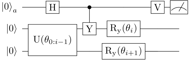
Figure 2: Quantum circuit $W_{2}(\bm{\theta})$ used to calculate the $2C_{i}$ term in the non-Hermitian case by separation of the TC Hamiltonian into Hermitian and anti-Hermitian parts. We define that $V=H$ and $V=R_{x}(\frac{\pi}{2})$ for the Hermitian and anti-Hermitian parts of a TC Hamiltonian, respectively. This circuit should be repeated for every term of the Hamiltonian. Note that no controlled Hamiltonian term is present.

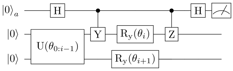
Figure 3: Quantum circuit $W_{1}(\bm{\theta})$ used to calculate the $2C_{i}$ term in the non-Hermitian case when, for simplicity, the Hamiltonian is given by a single Pauli on the $i$-th qubit, $\hat{H}=1^{(0)}\otimes...\otimes 1^{(i-1)}Z^{(i)}1^{(i+1)}\otimes...\otimes 1^{(N_{q}-1)}$ (controlled Z-gate) where $N_{q}$ denotes the number of qubits. This circuit should be repeated and adapted for every term of the Hamiltonian (controlled Pauli string) leading to $\mathcal{O}(N^{6})$ different circuits to be measured in TC cases.

However, in the TC case, $\hat{H}_{tc}$ is non-Hermitian and therefore such approach is not applicable. Recently, McArdle et al. McArdle and Tew (2020) proposed a method for the evaluation of the matrix elements $A_{ij}$ and $C_{i}$. To compute $C_{i}$ elements, they make use of independent circuits $W_{1}(\bm{\theta})$, which include control operations associated to each term of the system Hamiltonian (see Fig. 3). Unfortunately, the costs associated to the implementation of the corresponding circuits in hardware calculations on current noisy quantum processors are prohibitively large and therefore not applicable in practice.

In this work, we designed instead a new strategy based on the decomposition of the non-Hermitian TC Hamiltonian into its Hermitian and anti-Hermitian components. We first define the two (Hermitian and anti-Hermitian) operators

$$\hat{H}_{tc}^{+} =\hat{H}_{tc}+\hat{H}_{tc}^{\dagger}\,,$$ (17)

$$\hat{H}_{tc}^{-} =\hat{H}_{tc}-\hat{H}_{tc}^{\dagger}\,.$$ (18)

We then compute the coefficients $C_{i}$ as

$$C_{i} =\frac{1}{2}(\langle\partial_{\theta_{i}}\Phi|\hat{H}_{tc}|\Phi\rangle+\langle\Phi|\hat{H}_{tc}^{\dagger}|\partial_{\theta_{i}}\Phi\rangle)=\frac{C^{+}_{i}+C^{-}_{i}}{4}\,,$$ (19)

where

$$C^{+}_{i} =\langle\partial_{\theta_{i}}\Phi|\hat{H}_{tc}^{+}|\Phi\rangle+\langle\Phi|\hat{H}_{tc}^{+}|\partial_{\theta_{i}}\Phi\rangle=2\Re\langle\partial_{\theta_{i}}\Phi|\hat{H}_{tc}^{+}|\Phi\rangle\,$$ (20)

and

$$C^{-}_{i} =\langle\partial_{\theta_{i}}\Phi|\hat{H}_{tc}^{-}|\Phi\rangle-\langle\Phi|\hat{H}_{tc}^{-}|\partial_{\theta_{i}}\Phi\rangle=2\Re\langle\partial_{\theta_{i}}\Phi|\hat{H}_{tc}^{-}|\Phi\rangle\,.$$ (21)

Following this strategy, we can now implement the calculation of vector elements $C_{i}$ using two circuits of the form $W_{2}(\bm{\theta})$ given in Fig. 2, one for the Hermitian, Eq. (20), and one for the anti-Hermitian, Eq. (21), component of the transcorrelated operator $\hat{H}_{tc}$. For detailed derivations, see Appendices E and F. The measurements of the $A_{ij}$ matrix elements are performed in the standard way (since they are independent of the Hamiltonian) and can be found in Refs. McArdle et al. (2020); Yuan et al. (2019).

IV Results and discussion

IV.1 Simulations

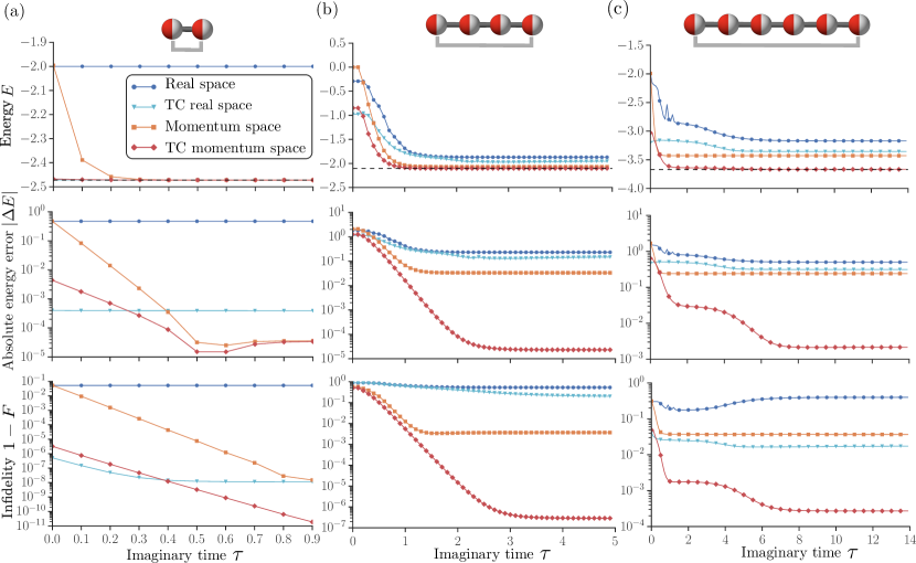
Figure 4: Results of QITE state-vector simulations of repulsive Hubbard models with (a) 2, (b) 4 and (c) 6 sites at half-filling with $t=1$ and $U=4$, using the qUCCSD ansatz with one layer. For every system, we report the evolution of the energy $E$ (top), absolute energy error $|\Delta E|=|E-E_{exact}|$ (middle) and infidelity $1-F$ (bottom) where the fidelity $F=|\langle\Phi|\Phi_{exact}\rangle|^{2}$ is computed with respect to the exact ground state at half-filling $|\Phi_{exact}\rangle$ of the corresponding Hamiltonian. The dashed lines represent the exact ground state energies, $E_{exact}$ $(-2.472,-2.103,-3.669$ respectively), for the three systems. (For the 6-site system, we only show every 5th data point for improved readability.) In most cases, the TC momentum-space method presents orders of magnitude improvement both in energy error and infidelity.

In this section, we demonstrate the advantages of using the transcorrelated versions of the Hubbard model both in the real and momentum space. As first accessible test cases, we considered the 2-, 4- and 6-site 1D Hubbard models. It is important to mention that due to hardware and software limitations, validation of quantum computing algorithms are currently restricted to rather small system sizes. For this reason, in this work we decided to restrict our self to the study of the 1D Hubbard model, even tough it is analytically solvable. Furthermore, accessible 2D systems like the $2\times 2$ and the $2\times 3$ lattice models are anyway dominated by finite size effects and can be recast into a folded 1D chain.

For each system, we perform QITE simulations to obtain a ground state estimate $\ket{\Phi}$ and quantify the performance in terms of the absolute energy error, $|\Delta E|=|E-E_{exact}|$, and the infidelity, $I=1-|\langle\Phi|\Phi_{exact}\rangle|$, with respect to the targeted exact ground states at half-filling. We denote the latter with $\ket{\Phi^{r}_{exact}}$ and $\ket{\Phi^{m}_{exact}}$ for the real- and the momentum-space representations, respectively, and compute them by exactly diagonalizing the corresponding Hamiltonian. Throughout the rest of this work, we assume that our results correspond to SV-type simulations unless specified otherwise and specify energies in units of the Hubbard parameter $t$. For each system, we initialize the QITE algorithm at the mean-field solution of the non-interacting ($U/t=0$) non-TC Hubbard model (Fermi-sea / Hartree-Fock solution). More specifically, the initial states of the calculations using the TC Hamiltonians are taken to be the same as for the non-TC cases and correspond to the $U/t=0$ solutions of the Hubbard Hamiltonians in the real space $\ket{\Phi^{r}_{0}}$ and the momentum space $\ket{\Phi^{m}_{0}}$. For hardware experiments, an inexpensive short-depth VQE calculation can be used for state initialization (i.e., $\ket{\Phi^{r/m}_{0}}\approx\min_{\bm{\theta}}\langle\Phi(\bm{\theta})|\hat{H}_{U=0}^{r/m}|\Phi(\bm{\theta})\rangle$) with a suitable ansatz and initial state (see Fig. 1(c)). To assess the optimal time-step $t_{s}$ for the QITE algorithm to reach the required accuracy, we performed series of SV test calculations, which led to a choice of $\Delta t_{s}=10^{-1}$ valid for all investigated systems. It is worth mentioning that the presence of the parametrized global phase can improve the results of QITE Yuan et al. (2019) in comparison to VQE, which is fully independent from the global phase. Other technical details are summarized in Sec. III.

In Fig. 4, we show the results of QITE simulations in SV formulation of a two-, four- and six-site repulsive Hubbard model with periodic boundary conditions at intermediate interaction strength, $U/t=4$.

After a first inspection, we can already advance the following general main observations: First, the QITE algorithm can be efficiently used to optimize the ground state of the Hubbard model, both in its original Hermitian formulation, as well as in the non-Hermitian TC form, in the real and momentum space. Secondly, we observe a clear advantage of the momentum-space representation of the Hubbard model in conjunction with the QITE algorithm (at least for this critical intermediate interaction strength regime). Finally, the transcorrelated formulation of both the real-space and, more strikingly, momentum-space Hubbard model leads to a faster and tighter convergence of the ground state energies and corresponding state fidelities.

IV.1.1 Advantages of the momentum representation

In all systems investigated (Fig. 4), we observe a fast relaxation from the initial state towards the optimized ground states, with the exception of the real-space representations (in blue), which remain stack at higher energy values due to the limitations of the wavefunction ansatz for this particular description of the problem. The reason for this behavior resides in the fact that the momentum representation allows for a more compact form of the wavefunction and therefore requires a shallower quantum circuit to describe the ground state wavefunction. In fact, in the real space, the qUCCSD ansatz is not expressive enough to span the portion of the Hilbert space that contains the ground state wavefunction. This behaviour is confirmed by VQE simulations, which reproduce equivalent results (see Fig. 5(a)).

The advantage of the momentum-space representation in the low-to-intermediate interaction strength regime is demonstrated by the fact that the final energy error (middle row in Fig. 4) both with and without the TC method, are lower than the corresponding real-space results for all lattice sizes. Except for the 6-site case, where the infidelity of the TC real-space result is lower than the non-TC momentum-space result (lower right panel of Fig. 4), all the state infidelities (bottom row) of the approximate ground state are lower in the momentum-space than in the real-space formulation. This exception shows that a larger infidelity of the ground state does not directly correspond to a large error in energy, as the momentum-space energy error in the 6-site case is still lower than the corresponding TC real-space result. Additionally, in all momentum-space simulations, with and without applying transcorrelation, the same qUCCSD ansatz used in the real space is capable of representing the ground state by improving on the initial state.

IV.1.2 Advantages of the transcorrelated formulation

As discussed in Section II, the use of the transcorrelated transformation can further simplify the structure of the many-electron wavefunction, making the mapping to a quantum circuit more efficient. As a consequence, with the TC Hamiltonian, the optimization converges to the approximate ground states with less resources (shallower circuits) than using the usual (non-TC) approach. Figs. 4 and 5 summarize all results for the optimization of the Hubbard models with 2, 4 and 6 sites. The optimization dynamics in Fig. 4 are given for a fixed depth ($n=1$) qUCCSD wavefunction ansatz, while Fig. 5 shows the converged values for the energy deviations and state infidelities as a function of the circuit depth ($n=1,2$), for the different Hamiltonian representations. In all cases, a maximum of 2 repetition layers was sufficient to achieve a tight convergence (i.e., high fidelities) at least for the TC cases.

The efficiency of the TC approach is a consequence of the extremely “compact” form of the exact right eigenvector (i.e. almost single reference) of the TC Hamiltonians, which are dominated by the ground states with the interaction term $U=0$, $\ket{\Phi^{r/m}_{0}}$, that were used as initial state in all QITE calculations (TC and non-TC). This effect is most pronounced for 2 sites, see Fig. 4(a), where for the TC Hamiltonians both in the real and momentum space, the starting states $\ket{\Phi^{r/m}_{0}}$ are already a reasonable approximation of the exact ground state characterized by energy deviations $|\Delta E|<10^{-3}$ and infidelities $I<10^{-5}$. Compared to the original real-space results, the energy error for the TC real-space case is reduced by three orders of magnitude from about $4\times 10^{-1}$ to $3\times 10^{-4}$ and, as in the purely real-space formulation, the value of the energy/infidelity is not improved over the whole duration of the QITE dynamics.

Also for the 4-site model (see Fig. 4(b)) the TC formulation of the Hamiltonian in the momentum space is the best method. The initial states $|\Phi^{r/m}_{0}\rangle$ provide an improved starting point upon non-TC methods (see initial energy values) and we observe significant improvements of the energies/infidelities due to QITE for all Hamiltonians. Most importantly, the Hamiltonian in the TC momentum-space representation offers approximately up to 4 and 7 orders of magnitude improvement in absolute energy error and infidelity, respectively, in comparison to the TC real-space representation.

In Fig. 4(c), we show the results for the largest 6-site system we studied in this work, presenting a challenge for QITE. All simulations, except the TC momentum-space ones, have significant residual energy errors $|\Delta E|>10^{-1}$ when using the standard qUCCSD ansatz. The presence of kinks at the beginning of the real-space simulation (blue circles) is due to the errors in the inversion of the linear system, Eq. (12), and are suppressed by means of the Tikhonov regularization at future time-steps. The TC momentum-space approach allows for at least 2 orders of magnitude improvement in energy error and infidelity with respect to all other approaches. Due to the inclusion of correlation directly into the TC Hamiltonian, it is the only approach which allows to resolve the exact ground state with a limited (in terms of expressibility) one-layer qUCCSD ansatz. A similar behavior was found in Dobrautz et al. Dobrautz et al. (2019a), where it was shown that a momentum-space TC Hubbard model can be accurately solved with a limited restricted configuration interaction approach that only includes up to quadruple excitation for a 18-site system.

The results in Fig. 4 confirm that there exists a clear advantage in the use the TC momentum-space formulation of the Hubbard model, while the TC real-space approach presents only minor improvements in comparison. The momentum-space TC results suggest that a less expressive ansatz, and thus a shallower quantum circuit, is required to obtain accurate results for the Hubbard model. For this reason, in Fig. 5, we report, as anticipated above, the converged results of QITE simulations when we double the number of layers in the qUCCSD ansatz by repeating it with independent variational parameters (doubling the number of parameters, denoted as 2-qUCCSD), and compare the results to the ones obtained with a single qUCCSD layer. In addition, to validate our results and highlight the potential advantage of the proposed TC approach combined with the QITE algorithm, we also perform VQE optimizations with the original real- and momentum-space Hubbard Hamiltonians (since the standard VQE is applicable only to Hermitian case).

As for the 2-site system (Fig. 5(a)), inclusion of a second layer in the qUCCSD ansatz improves the circuit expressibility leading to a drastic improvement of the real-space results (dark blue), where the energy error drops from $4\times 10^{-1}$ for 1 layer to below $10^{-4}$ for 2 layers. Similarly, the energy error of the TC real space (light blue) and the TC momentum space (red) is reduced by more than 2 orders of magnitude upon inclusion of a second qUCCSD layer and all approaches achieve a staggeringly small infidelity of $10^{-14}$. The original momentum-space results (orange) do not improve upon adding an extra quantum circuit layer. However, this is consistent with the benchmark VQE calculations (black lines in Fig. 5) that we performed for the real- and momentum-space Hubbard models.

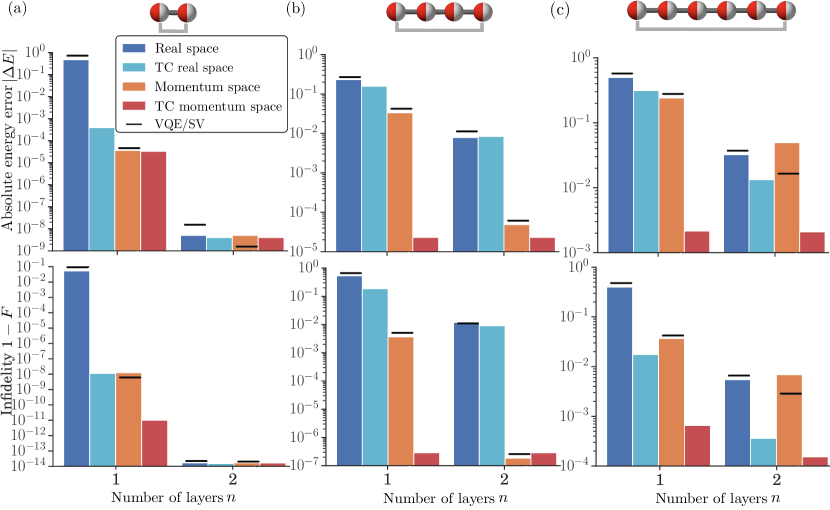
Figure 5: Results of QITE state-vector simulations of repulsive Hubbard models with (a) 2, (b) 4 and (c) 6 sites at half-filling with $t=1$ and $U=4$, using the qUCCSD ansatz with $n$ layers. For every system, we report the absolute energy error $|\Delta E|=|E-E_{exact}|$ (top) and the infidelity $1-F$ (bottom) at convergence, where the fidelity $F=|\langle\Phi|\Phi_{exact}\rangle|^{2}$ is computed with respect to the exact ground state at half-filling $|\Phi_{exact}\rangle$ of the corresponding Hamiltonian. The solid lines mark the converged outcomes of VQE state-vector simulations (VQE/SV) for the real/momentum-space Hamiltonians. The benefits of the transcorrelated approach can be seen, for instance, in the result of the 6-site TC momentum-space Hamiltonian with $n=1$, which is significantly more accurate than the plain momentum-space outcome with $n=2$, especially in terms of fidelity.

The same trend is also confirmed for larger systems (see Fig. 5, panels (b) and (c)). In fact, for all Hamiltonian representations with the exception of the TC momentum-space one, we observe a reduction of absolute energy error (about 1-3 orders of magnitude) and of the infidelities (about 2-4 orders of magnitude) when a second layer is added to the wavefunction ansatz. Note that the quality of the momentum-space TC results (in red) with a single qUCCSD layer is significantly better ($|\Delta E|\lesssim 10^{-3}$) than the one obtained with all other approaches, even when in these cases 2 layers of the qUCCSD ansatz are used. The same is true when we compared the converged momentum-space TC values with the results obtained with VQE using the real- and momentum-space (non-TC) Hamiltonians (black lines). This is a very important result in view of future applications of this approach in near-term quantum computing.

To summarize, the inclusion of correlation directly into the TC Hamiltonian via the similarity transformation based on a Gutzwiller ansatz allows us to obtain highly accurate results using the QITE algorithm with very shallow circuits (1-layer qUCCSD), in particular when the momentum-space representation of the Hubbard model is used.

IV.2 Hardware calculations

Figure 6: Results of QITE simulations of the repulsive 2-site Hubbard model at half-filling with $U/t=4$. The RY heuristic ansatz (applied to the Hartree-Fock state), consisting of one layer with linear entanglement, is used, see Fig. 1(c). We report the evolution of the energy $E$ (top) and absolute energy error $|\Delta E|=|E-E_{exact}|$ (bottom) computed with respect to the exact ground state at half-filling $|\Phi_{exact}\rangle$ of the corresponding Hamiltonian. The dashed line represents the exact ground state energy $E_{exact}=-2.472$. HW denotes the simulations performed on the ibmq_lima quantum computer. QASM marks the classical noisy simulations with the noise model of the ibmq_lima chip. (Only every second data point is shown to improve the readability.)

Due to the limited number of available qubits, we only performed hardware (HW) experiments for the 2-site Hubbard model. Consequently, based on the results of Fig. 5a, we opted for the study of the real-space Hubbard model, since it shows a noticeable effect on the accuracy (see blue and teal bars) when the TC method is applied for a single UCCSD Ansatz layer. On the other hand, the momentum-space results for the 2-site model show similar accuracy for both TC and non-TC approaches. Before moving to HW experiments, we performed QASM simulations (see Ref. Sokolov et al. (2021) for some examples) of the QITE algorithm, which include statistical measurement noise as well as a noise model tuned for the particular IBM quantum computer used in this paper, namely ibmq_lima (see Fig. 1(a)). Details about the quantum device and the noise model used are given in Appendix G.

As mentioned above, due to its large circuit depth the qUCCSD ansatz is not usable for current HW experiments, due to limited coherence time and gate errors. Thus, in both QASM and HW simulations, we used the hardware-efficient heuristic RY ansatz Kandala et al. (2017); Barkoutsos et al. (2018) applied to the Fermi-sea / Hartree-Fock initial state $\ket{\Phi^{r}_{0}}$. For more details on the nature of the wavefunction ansatz see Appendix D. Furthermore, these new calculations confirm that the proposed TC approach is not restricted to a specific wavefunction ansatz. (On the other hand, this is also the reason why the initial state and the corresponding initial energies are different compared to the ones seen in the SV simulations.) The quantum circuit used for the HW calculations is given in Fig. 1(c).

Fig. 6 shows the evolution of the total energies and absolute energy errors for the QASM simulations (pink and magenta) and the HW experiments (light and dark blue) as a function of imaginary time. Both the ordinary and TC QITE/QASM results are in qualitative agreement with SV results reported in Fig. 4(a), even though – as expected – the accuracy is reduced by the presence of a realistic noise model. Surprisingly, the HW calculations converge faster than the corresponding QASM noisy simulations, demonstrating that noise is not necessarily deteriorating the results. In all cases, the TC approaches converge faster than the corresponding Hermitian cases. On the other hand, achieving a tight convergence (with energy errors less than $10^{-2}$) in the presence of noise is harder and therefore – to limit the costs of the calculations – we stopped all HW experiments when no further significant improvement of the energy was noticed (hence the different duration of the simulations). The qualitative good match between the converged solutions of QASM and HW experiments demonstrate that the TC approach is not only compatible with a simpler wavefunction ansatz but also leads to a noise resilient implementation of the QITE algorithm.

V Conclusions and outlook

In this paper, we demonstrated the advantages of using the transcorrelated (TC) formulation of the Hubbard Hamiltonian both in real- and momentum-space representations. One of the strengths of our approach resides in the absence of approximations in the derivation and the implementation of the TC Hamiltonian together with the efficient classical optimization of the Gutzwiller factor. The difficulties posed by the non-Hermiticity of TC Hamiltonians are overcome by using the quantum imaginary time evolution (QITE) algorithm. In particular, we performed state-vector QITE simulations (without statistical and hardware noise) of 2-, 4- and 6-site Hubbard models, showing that the TC method in the momentum space offers up to 4 orders of magnitude improvement of the absolute energy error for a fixed ansatz in comparison to the non-TC approaches.

To demonstrate the validity of our approach on a quantum computer, we propose a hardware-efficient implementation of the QITE algorithm in quantum circuits tailored to non-Hermitian Hamiltonians. We showed that QITE in the non-Hermitian case can be performed using the standard approach, differentiation of general gates via a linear combination of unitaries Schuld et al. (2019), by separating the Hamiltonian into Hermitian and non-Hermitian parts. This is in contrast with the suggestion of McArdle et al. McArdle and Tew (2020) where different quantum circuits for each term in the Hamiltonian (i.e., controlled Hamiltonian terms) are required. Our implementation is tested by performing realistic quantum circuit (QASM) simulations for 2-site Hubbard model, including the statistical error and noise sources modeled after the ibmq_lima quantum computer. Moreover, we further confirm our methodology by performing the same experiments on the actual ibmq_lima chip. The converged results are in qualitative agreement with QASM and SV simulations.

Concerning the scaling of the TC methods of this work, the presence of three-body interactions in TC Hamiltonians increases the number of required measurements on quantum hardware from a $\mathcal{O}(N^{4})$ scaling for non-TC Hamiltonians to a $\mathcal{O}(N^{6})$ scaling, with $N$ being the total number of sites. This poses a potential challenge for applying such TC methods in near-term noisy quantum computers. However, Pauli grouping Gokhale et al. (2019); Yen et al. (2020); Crawford et al. (2021); van den Berg and Temme (2020) and positive operator-valued measure García-Pérez et al. (2021) methods could optimize the measurement process and further reduce the number of measurements. More detailed investigations are required in order to better assess the validity these approaches, which implementation goes beyond the scope of this work.

In conclusion, despite the increased number of measurements due to the presence of three-body terms, the TC approaches studied in this work significantly improve the accuracy of our calculations by making the ground state extremely “compact” and enable the use of shallower quantum circuits as wavefunction ansatzes, compatible with near-term noisy quantum computers. The established methodology paves the way for applications to ab initio Hamiltonians Cohen et al. (2019), bringing closer the first relevant demonstration of quantum advantage in a relevant use-case in the field of quantum chemistry.

VI Acknowledgements

I.O.S and I.T. gratefully acknowledge the financial support from the Swiss National Science Foundation (SNF) through the grant No. 200021-179312. W.D., H.L. and A.A. gratefully acknowledge financial support from the Max Planck society. We thank Jürg Hutter, Julien Gacon, Christa Zoufal, Max Rossmanek, Guglielmo Mazzola and Daniel Miller for fruitful discussions. IBM, the IBM logo, and ibm.com are trademarks of International Business Machines Corp., registered in many jurisdictions worldwide. Other product and service names might be trademarks of IBM or other companies. The current list of IBM trademarks is available at https://www.ibm.com/legal/copytrade Funded by the European Union. Views and opinions expressed are however those of the author(s) only and do not necessarily reflect those of the European Union or REA. Neither the European Union nor the granting authority can be held responsible for them. W.D. acknowledges funding from the Horizon Europe research and innovation program of the European Union under the Marie Skłodowska-Curie grant agreement no. 101062864.

Appendix A Quantum gates

The unitary matrix representation of the most general single-qubit gate, which allows us to obtain any quantum state on the Bloch sphere, can be written as

$$U(\theta,\phi,\lambda)=\left(\begin{array}[]{cc}\cos\left(\frac{\theta}{2}\right)&-e^{i\lambda}\sin\left(\frac{\theta}{2}\right)\\ e^{i\phi}\sin\left(\frac{\theta}{2}\right)&e^{i(\phi+\lambda)}\cos\left(\frac{\theta}{2}\right)\end{array}\right)\,.$$ (22)

Frequently, the gates that perform the rotations around the $x$-, $y$- and $z$-axis on the Bloch sphere are particularly useful in heuristic ansatzes (see Fig. 1(c)) and are given by:

$$R_{x}(\theta)=U\left(\theta,-\frac{\pi}{2},\frac{\pi}{2}\right)\,,$$ (23)

$$R_{y}(\theta)=U(\theta,0,0)\,,$$

$$R_{z}(\lambda)=e^{-i\lambda/2}U(0,0,\lambda)\,.$$

The X-gate allows us to construct the initial state $|\Phi_{0}\rangle=|0101\rangle$ in Fig. 1(c), and is given by $U\left({\pi},0,{\pi}\right)$.

Appendix B Tikhonov regularization

In this work, we combined the Tikhonov regularization approach with the implementation of the QITE algorithm, as suggested in Ref. McArdle et al. (2019b). The solution of the linear system $\bm{A}{\bm{\dot{\theta}}}=-\bm{C}$ at each time-step of QITE requires the inversion of the matrix $\bm{A}$ (see Eq. (15)) which is prone to be ill-conditioned. In addition, problems can occur due to the presence of hardware noise and statistical error originated from a finite number of measurements in the computation of the $A_{ij}$ matrix elements, see Eq. (13). Instead, we use the aforementioned regularization to update the parameters $\bm{{\theta}}$, which minimizes

$$\|\bm{C}+\bm{A}\bm{\dot{\theta}}\|^{2}+\lambda\|\bm{\dot{\theta}}\|^{2}.$$ (24)

The Tikhonov parameter $\lambda\in\mathbb{R}$ can be tuned to provide a smoother evolution of the parameters $\bm{\theta}$ (i.e., when $\lambda$ is large) in detriment of the accuracy (i.e., when $\lambda$ is small). The optimal regularization parameter $\lambda_{opt}$ can be efficiently found at each time-step by finding the “corner” of an L-curve in certain interval for $\lambda$ Cultrera and Callegaro (2020). For all simulations and experiments, we use $\lambda\in[10^{-3},1]$ and the termination threshold of the L-curve corner search set to $10^{-8}$. In our experience, those parameters provided the best results.

Appendix C Optimization of $J$

As mentioned in Sec. III, the optimization of the Gutzwiller parameter $J$ based on a projection method is similar to the solution of a coupled cluster amplitudes equation Taylor (1994). We start from a general single determinant eigenvalue equation

$$\hat{H}_{tc}(J)\ket{\Phi_{0}}=E\ket{\Phi_{0}},$$ (25)

where the explicit dependence of $\hat{H}_{tc}$ on the parameter $J$ is indicated and $\ket{\Phi_{0}}$ denotes the HF/Fermi-sea determinant. If we project Eq. (25) onto $\bra{\Phi_{0}}$,

$$\langle{\Phi_{0}}|{\hat{H}_{tc}}|{\Phi_{0}}\rangle=E_{0}(J),$$ (26)

we obtain an expression of the TC “Hartree-Fock” energy, which depends on the parameter $J$. Projecting Eq. (25) onto $\bra{\Phi_{0}}\hat{g}(J)$ yields

$$\langle{\Phi_{0}}|{\hat{g}\hat{H}_{tc}(J)}|{\Phi_{0}}\rangle= \langle{\Phi_{0}}|{\hat{g}E}|{\Phi_{0}}\rangle$$

$$= E_{0}(J)\langle{\Phi_{0}}|{\hat{g}}|{\Phi_{0}}\rangle.$$ (27)

Then, combining Eq. (26) and (C) yields

$$\langle{\Phi_{0}}|{\left(\hat{g}-\left\langle{\hat{g}}\right\rangle_{0}\right)\hat{H}_{tc}(J)}|{\Phi_{0}}\rangle=0,$$ (28)

where $\left\langle{\hat{g}}\right\rangle_{0}=\langle{\Phi_{0}}|{\hat{g}}|{\Phi_{0}}\rangle$ and $\hat{g}$ is expressed in the momentum space

$$\hat{g}=\frac{J}{N}\sum_{\mathbf{p,q,k},\sigma}c_{\mathbf{p-k},\sigma}^{\dagger}c_{\mathbf{q+k},\bar{\sigma}}^{\dagger}c_{\mathbf{q},\bar{\sigma}}c_{\mathbf{p},\sigma}.$$ (29)

Eq. (28) can be efficiently solved for $J$ with a mean-field level computational cost. To see the connection to coupled cluster theory: Eq. (28) can also be interpreted as a projection of the eigenvalue equation $(\hat{H}_{tc}-E)\ket{\Phi_{0}}=0$ on the single basis of the correlation factor $\hat{g}$; the parameter $J$ can be interpreted as the sole and uniform amplitude of a coupled cluster ansatz (Eq. (29)). The specific values obtained by solving Eq. (28), $J_{proj}$, and VMC optimized results, $J_{VMC}$, for the lattice sizes, fillings and $U/t$ values used in this study are listed in Table 1. As already studied in Ref. (76), too large values of $J$ can cause instabilities in the imaginary time evolution due to a resulting wide span in magnitude of the off-diagonal matrix elements after the similarity transformation. For this reason we chose slightly smaller values than $J_{proj}$ would suggest (see $J_{QITE}$ values in Tab. 1). This still causes a more “compact” right eigenvector, while having a positive influence on the stability of the QITE algorithm.

Table 1: Optimized Gutzwiller parameters obtained by projection, $J_{proj}$, and VMC optimization, $J_{VMC}$, for the
$2$-, $4$- and 6-site Hubbard model at half-filling and $U/t=4$. $J_{QITE}$ denotes the Gutzwiller parameters that are used in our QITE simulations and experiments.

Number of sites	2	4	6
$J_{proj}$	-0.48	-0.88	-0.67
$J_{VMC}$	-0.47	-1.00	-0.76
$J_{QITE}$	-0.48	-0.73	-0.59

Appendix D qUCCSD and heuristic RY ansatzes

The qUCCSD wavefunction ansatz Peruzzo et al. (2014)

$$|\Phi(\bm{\theta})\rangle=\hat{U}^{(n)}_{ucc}(\bm{\theta})|\Phi_{0}\rangle\,,$$ (30)

has seen great success in providing accurate results when embedded in variational quantum algorithms, such as VQE and QITE, to prepare the ground state of molecular Barkoutsos et al. (2018); Romero et al. (2018); Sokolov et al. (2020); Gomes et al. (2020) and condensed matter Hamiltonians Cade et al. (2020); Xu et al. (2020); Bonet-Monroig et al. (2021). The corresponding cluster operator is given by a Trotterized version of the UCCSD operator Hoffmann and Simons (1988)

$$\begin{split}\hat{U}^{(n)}_{ucc}(\bm{\theta})&=\prod_{n}\left(\prod_{ij}\exp{\left(\theta^{n}_{ij}(\hat{a}_{i}^{\dagger}\hat{a}_{j}-\hat{a}_{j}^{\dagger}\hat{a}_{i})\right)}\right.\\ &\left.\times\prod_{ijkl}\exp{\left(\theta^{n}_{ijkl}(\hat{a}^{\dagger}_{i}\hat{a}^{\dagger}_{j}\hat{a}_{k}\hat{a}_{l}-\hat{a}^{\dagger}_{l}\hat{a}^{\dagger}_{k}\hat{a}_{j}\hat{a}_{i})\right)}\right)\,,\end{split}$$ (31)

where, for this work, we also consider $n$ independent layers (referred to as n-qUCCSD) and all singles and doubles excitations from the Fermi-sea/Hartree-Fock state. By mapping the fermionic operators to qubits using the Jordan-Wigner transformation, corresponding quantum circuits Barkoutsos et al. (2018) can be derived with the number of parameters scaling as $\mathcal{O}(nN_{q}^{2}N_{e}^{2})$ and number of gates scaling as $\mathcal{O}(nN_{q}^{3}N_{e}^{2})$ where $N_{e}$ and $N_{q}$ are, respectively, the numbers of electrons and qubits Romero et al. (2018). Despite a significant number of gates for current noisy quantum processors, the attractive quality of the qUCCSD ansatz resides in the guarantee of a reasonable approximation to the solution of quantum many-body problems.

To perform the experiments on quantum computers, we also employ a variant of the heuristic hardware-efficient wavefunction ansatzes, which were introduced in Kandala et al. (2017), that can be written as

$$|\Phi(\bm{\theta})\rangle=\hat{U}^{(n)}_{heu}(\bm{\theta})|\Phi_{0}\rangle=\prod_{n}\left(\hat{U}_{ent}\hat{U}_{rot}(\bm{\theta})\right)|\Phi_{0}\rangle\,,$$ (32)

where multiple layers are combined, consisting of alternating blocks of arbitrary parametrized single-qubit rotations $\hat{U}_{rot}(\bm{\theta})$ and entangling blocks $\hat{U}_{ent}$ composed of arbitrary arrangement of two-qubit gates. Note that the vector $\bm{\theta}$ includes the parameters from all $n$ layers. The selection of single-qubit gates and entangling gates is typically performed to make the quantum circuit shallow enough to fit in the limits of the corresponding quantum computer. An example of such ansatz is given in Fig. 1(c), where we employ two rotation layers $\hat{U}_{rot}(\bm{\theta})=\bigotimes^{N_{q}-1}_{i=0}R_{y}(\theta_{i})$ composed of $R_{y}(\theta_{i})$ rotations on each $i$-th qubit, separated by a entangling layer, $\hat{U}_{ent}=\prod_{i=0}^{N_{q}-2}\rm{CNOT}(i,i+1)$, where the first parameter denotes the control qubit and the second denotes the target qubit. The initial state is a single reference state $|0101\rangle$ constructed by applying $U(\pi,0,\pi)=X$, the Pauli-X gate (see Appendix A).

Table 2: Numbers of variational parameters in the wavefunction ansatzes used for different $N$-site Hubbard models. An additional variational parameter is used to track the global phase in QITE simulations.

Number of sites	2	4	6
qUCCSD	3	26	117
2-qUCCSD	6	52	234
RY	8	-	-

In general, for heuristic ansatzes it is unclear what number of layers $n$ is required to achieve highly accurate results. Progresses to alleviate this problem have been made with additions to variational quantum frameworks of adaptive Grimsley et al. (2019); Tang et al. (2021); Yordanov et al. (2021) and evolutionary methods Rattew et al. (2019); Chivilikhin et al. (2020) for the ground state preparation, to name only a few. Moreover, Hamiltonian-inspired ansatzes were shown to provide benefits in comparison to the qUCCSD ansatz for Hubbard models in terms of reduced number of variational parameters but also requiring the tuning of the number of layers as for heuristic ansatzes Wecker et al. (2015); McArdle and Tew (2020). In the context of transcorrelated Hamiltonians, an ansatz based on the repeated layers of a Trotterised decomposition of the time evolution operator $\exp[-{i}\hat{H}t]$ has been used, where a variational parameter $\theta$ is associated to every Hamiltonian term McArdle and Tew (2020). However, this ansatz is inappropriate for current noisy quantum computers in comparison to the qUCCSD ansatz due to the worse scaling of the number of variational parameters in $\mathcal{O}(N^{6})$ (i.e., the number of terms in TC Hamiltonians, see Section II.2). Therefore, in this work, we focus on the most simple and validated approaches (e.g., the qUCCSD and hardware-efficient ansatzes) that allow us to showcase the benefits of exact TC methods. The specific number of parameters of the different used ansatzes in this work are shown in Table 2.

Appendix E Computation of C vector elements

We first define the Hermitian $\hat{H}_{tc}^{+}$ and the anti-Hermitian $\hat{H}_{tc}^{-}$ operators derived from the non-Hermitian TC Hamiltonian $\hat{H}_{tc}\in\{\hat{H}^{r}_{tc},\hat{H}^{m}_{tc}\}$:

$$\hat{H}_{tc}^{+} =\hat{H}_{tc}+\hat{H}_{tc}^{\dagger}\,,$$ (33)

$$\hat{H}_{tc}^{-} =\hat{H}_{tc}-\hat{H}_{tc}^{\dagger}\,,\$$ (34)

with $\hat{H}_{tc}^{+\dagger}=\hat{H}_{tc}^{+}$ and $\hat{H}_{tc}^{-\dagger}=-\hat{H}_{tc}^{-}$.

Then, we can write

$$\langle\partial_{\theta}\Phi|\hat{H}_{tc}^{+}|\Phi\rangle +\langle\Phi|\hat{H}_{tc}^{+\dagger}|\partial_{\theta}\Phi\rangle$$

$$=\langle\partial_{\theta}\Phi|\hat{H}_{tc}^{+}|\Phi\rangle+(\langle\partial_{\theta}\Phi|\hat{H}_{tc}^{+}|\Phi\rangle)^{*}$$

$$=2\Re\langle\partial_{\theta}\Phi|\hat{H}_{tc}^{+}|\Phi\rangle$$ (35)

and

$$\langle\partial_{\theta}\Phi|\hat{H}_{tc}^{-}|\Phi\rangle +\langle\Phi|\hat{H}_{tc}^{-\dagger}|\partial_{\theta}\Phi\rangle$$

$$=\langle\partial_{\theta}\Phi|\hat{H}_{tc}^{-}|\Phi\rangle+(\langle\partial_{\theta}\Phi|\hat{H}_{tc}^{-}|\Phi\rangle)^{*}$$

$$=2\Re\langle\partial_{\theta}\Phi|\hat{H}_{tc}^{-}|\Phi\rangle\,.$$ (36)

Using the (anti-)hermiticity, we obtain

$$\langle\partial_{\theta}\Phi|\hat{H}_{tc}^{+}|\phi\rangle+\langle\Phi|\hat{H}_{tc}^{+}|\partial_{\theta}\Phi\rangle =2\Re\langle\partial_{\theta}\Phi|\hat{H}_{tc}^{+}|\Phi\rangle\,,$$ (37)

$$\langle\partial_{\theta}\Phi|\hat{H}_{tc}^{-}|\Phi\rangle-\langle\Phi|\hat{H}_{tc}^{-}|\partial_{\theta}\Phi\rangle =2\Re\langle\partial_{\theta}\Phi|\hat{H}_{tc}^{-}|\Phi\rangle\,.$$ (38)

Combining Eqs. (37) and (38), one gets

$$\langle\partial_{\theta}\Phi|\hat{H}_{tc}^{+} +\hat{H}_{tc}^{-}|\Phi\rangle+\langle\Phi|\hat{H}_{tc}^{+}-\hat{H}_{tc}^{-}|\partial_{\theta}\phi\rangle$$

$$=2\Re\langle\partial_{\theta}\Phi|\hat{H}_{tc}^{+}|\Phi\rangle+2\Re\langle\partial_{\theta}\Phi|\hat{H}_{tc}^{-}|\Phi\rangle$$ (39)

which implies

$$\langle\partial_{\theta}\Phi|2\hat{H}_{tc}|\Phi\rangle +\langle\Phi|2\hat{H}_{tc}^{\dagger}|\partial_{\theta}\Phi\rangle$$

$$=2\Re\langle\partial_{\theta}\Phi|\hat{H}_{tc}^{+}|\Phi\rangle+2\Re\langle\partial_{\theta}\Phi|\hat{H}_{tc}^{-}|\Phi\rangle\,.$$ (40)

Inserting the definitions in Eq. (17) and (18) and dividing by 2, we finally get

$$\langle\partial_{\theta}\Phi|\hat{H}_{tc}|\Phi\rangle +\langle\Phi|\hat{H}_{tc}^{\dagger}|\partial_{\theta}\Phi\rangle$$

$$=\Re\langle\partial_{\theta}\Phi|\hat{H}_{tc}^{+}|\Phi\rangle+\Re\langle\partial_{\theta}\Phi|\hat{H}_{tc}^{-}|\Phi\rangle\,,$$ (41)

which proves Eq. (19).

Appendix F Quantum circuit for the C vector elements

As mentioned in Sec. III, we derive the quantum circuits that are proposed to measure the elements of the gradient vector $\bm{C}$ in the QITE algorithm (see Fig. 2). In particular, we explain how to construct the quantum circuits that are compatible with the measurements of the (anti-)Hermitian terms contained in ($\hat{H}_{tc}^{-}$) $\hat{H}_{tc}^{+}$. To this end, we follow closely the derivations made for the Hermitian case in Ref. Schuld et al. (2019) using the linear combination of unitaries approach. Consider the case of the heuristic RY ansatz as used in our QASM and hardware experiments. To compute a derivative with respect to some gate parameter $\theta_{i}$ of the RY ansatz, we make use of a single ancilla qubit. We show how the quantum circuit for the anti-Hermitian case (see Fig. 2 with $V=R_{x}(\frac{\pi}{2})$) can be derived. First, we write the initial state of our quantum register as

$$|0\rangle_{a}\otimes|0\rangle\,.$$ (42)

By applying a Hadamard gate on the ancilla qubit, with its unitary matrix

$$H=\frac{1}{\sqrt{2}}\begin{pmatrix}1&1\\ 1&-1\\ \end{pmatrix}\,,$$ (43)

we obtain the state

$$\frac{1}{\sqrt{2}}(|0\rangle_{a}+|1\rangle_{a})\otimes|0\rangle\,.$$ (44)

We add a part of the ansatz circuit that comes before the differentiated gate, obtaining the state

$$\frac{1}{\sqrt{2}}(|0\rangle_{a}+|1\rangle_{a})\otimes U(\theta_{0:i-1})|0\rangle\,.$$ (45)

According to Schuld et al. Schuld et al. (2019), a derivative of the gate $\bar{G}$ can be decomposed into a linear combination of unitary gates $Q_{1}$ and $Q_{2}$ as

$$\partial_{\theta_{i}}{\bar{G}}=\frac{\alpha}{2}\left(\left(Q_{1}+Q_{1}^{\dagger}\right)+i\left(Q_{2}+Q_{2}^{\dagger}\right)\right),$$ (46)

with a parameter $\alpha\in\mathbb{R}$. For instance, for a gate $R_{y}(\theta_{i})$ of the RY ansatz, as in Fig. 2, $\partial_{\theta_{i}}\bar{G}=\beta R_{y}(\theta_{i})C_{Y}$ with $\beta=-\frac{1}{2}i$. $C_{Y}$ is a controlled-Y gate where Y stands for the Pauli operator $\hat{\sigma}_{y}$. This decomposition is performed automatically in Qiskit. The state of the circuit then becomes

$$\frac{1}{\sqrt{2}}[|0\rangle_{a}\otimes U(\theta_{0:i-1})|0\rangle+|1\rangle_{a}\otimes\beta YU(\theta_{0:i-1})|0\rangle]\,,$$ (47)

Then, we add the $R_{y}(\theta_{i})$ and $R_{y}(\theta_{i+1})$ gates to the circuit, as in Figure 2:

$$\frac{1}{\sqrt{2}}[|0\rangle_{a}\otimes R_{y}(\theta_{i+1})R_{y}(\theta_{i})U(\theta_{0:i-1})|0\rangle$$

$$+|1\rangle_{a}\otimes R_{y}(\theta_{i+1})R_{y}(\theta_{i})\beta YU(\theta_{0:i-1})|0\rangle]\,.$$ (48)

For compactness, we rewrite $\partial_{\theta_{i}}G=\beta R_{y}(\theta_{i})Y$ and $U(\theta_{0:i})=R_{y}(\theta_{i+1})R_{y}(\theta_{i})U(\theta_{0:i-1})$ and obtain

$$\frac{1}{\sqrt{2}}[|0\rangle_{a}\otimes U(\theta_{0:i})|0\rangle$$

$$+|1\rangle_{a}\otimes R_{y}(\theta_{i+1})\partial_{\theta_{i}}{G}U(\theta_{0:i-1})|0\rangle]\,.$$ (49)

Next, we apply the $R_{x}(\frac{\pi}{2})$ gate, with its unitary matrix

$$R_{x}\left(\frac{\pi}{2}\right)=\frac{1}{\sqrt{2}}\begin{pmatrix}1&-i\\ -i&1\\ \end{pmatrix}\,,$$ (50)

on the ancilla qubit, obtaining

$$\frac{1}{{2}}[(|0\rangle_{a}-i|1\rangle_{a})\otimes U(\theta_{0:i})|0\rangle$$

$$+(-i|0\rangle_{a}+|1\rangle_{a})\otimes R_{y}(\theta_{i+1})\partial_{\theta_{i}}{G}U(\theta_{0:i-1})|0\rangle]\,,$$ (51)

which can be written as

$$\frac{1}{{2}}[|0\rangle_{a}\otimes(U(\theta_{0:i})-iR_{y}(\theta_{i+1})\partial_{\theta_{i}}{G}U(\theta_{0:i-1}))|0\rangle$$

$$+|1\rangle_{a}\otimes(-iU(\theta_{0:i})+R_{y}(\theta_{i+1})\partial_{\theta_{i}}{G}U(\theta_{0:i-1}))|0\rangle]\,.$$ (52)

Therefore, if the ancilla qubit is measured in the state $|0\rangle_{a}$, we obtain the state

$$|\Psi_{0}\rangle=\frac{1}{{2\sqrt{p_{0}}}}\underbrace{[U(\theta_{0:i})-iR_{y}(\theta_{i+1})\partial_{\theta_{i}}{G}U(\theta_{0:i-1})]}_{R_{0}}|0\rangle\,,$$ (53)

and if it is measured in the state $|1\rangle_{a}$, we obtain the state

$$|\Psi_{1}\rangle=\frac{1}{{2\sqrt{p_{1}}}}\underbrace{[-iU(\theta_{0:i})+R_{y}(\theta_{i+1})\partial_{\theta_{i+1}}{G}U(\theta_{0:i-1})]}_{R_{1}}|0\rangle\,,$$ (54)

where $p_{i}=\frac{1}{{4}}\langle 0|R^{\dagger}_{i}R_{i}|0\rangle$ for $i\in\{0,1\}$. To obtain the $C^{-}_{i}$ vector elements (see Eq. (21)), we can combine such measurements in the following way: If we measure our Hamiltonian and the ancilla is in the state $|0\rangle_{a}$, we get

$$\langle\Psi_{0}|\hat{H}^{-}_{tc}|\Psi_{0}\rangle =\frac{1}{{4p_{0}}}\Big{[}\langle 0|(U(\theta_{0:i})^{\dagger}$$ (55)

$$+ iU(\theta_{0:i-1})^{\dagger}\partial_{\theta{i}}{G}^{\dagger}R_{y}(\theta_{i+1})^{\dagger})\hat{H}^{-}_{tc}(U(\theta_{0:i})$$

$$- iR_{y}(\theta_{i+1})\partial_{\theta_{i}}{G}U(\theta_{0:i-1}))|0\rangle\Big{]}$$

and if the ancilla is in the state $|1\rangle_{a}$, we get

$$\langle\Psi_{1}|\hat{H}^{-}_{tc}|\Psi_{1}\rangle =\frac{1}{{4p_{1}}}\Big{[}\langle 0|(iU(\theta_{0:i})^{\dagger}$$ (56)

$$+U(\theta_{0:i-1})^{\dagger}\partial_{\theta{i}}{G}^{\dagger}R_{y}(\theta_{i+1})^{\dagger})\hat{H}^{-}_{tc}(-iU(\theta_{0:i})$$

$$+R_{y}(\theta_{i+1})\partial_{\theta{i}}{G}U(\theta_{0:i-1}))|0\rangle\Big{]}\,.$$

As we want to keep the term $\langle 0|(U(\theta_{0:i-1})^{\dagger}\partial_{\theta{i}}{G}^{\dagger}R_{y}(\theta_{i+1})^{\dagger})\hat{H}^{-}_{tc}U(\theta_{0:i})|0\rangle=\langle\partial_{i}\Psi|\hat{H}^{-}_{tc}|\Psi\rangle$, we can subtract Eq. (55) from Eq. (56), including also the probabilities, to obtain

$$p_{0}\langle \Psi_{0}|\hat{H}^{-}_{tc}|\Psi_{0}\rangle-p_{1}\langle\Psi_{1}|\hat{H}^{-}_{tc}|\Psi_{1}\rangle$$ (57)

$$=\frac{i}{{2}}\Big{[} -\langle 0|U(\theta_{0:i})^{\dagger}\hat{H}^{-}_{tc}R_{y}(\theta_{i+1})\partial_{\theta{i}}{G}U(\theta_{0:i-1})|0\rangle$$

$$+\langle 0|U(\theta_{0:i-1})^{\dagger}\partial_{\theta{i}}{G}^{\dagger}R_{y}(\theta_{i+1})^{\dagger}\hat{H}^{-}_{tc}U(\theta_{0:i})|0\rangle\Big{]}\,.$$

Finally, multiplying by the factor $-2i$, we obtain $C^{-}_{i}$:

$$-2i\Big{[}p_{0}\langle\Psi_{0}|\hat{H}^{-}_{tc}|\Psi_{0}\rangle -p_{1}\langle\Psi_{1}|\hat{H}^{-}_{tc}|\Psi_{1}\rangle\Big{]}$$ (58)

$$=\langle\partial_{\theta_{i}}\Phi|\hat{H}^{-}_{tc}|\Phi\rangle-\langle\Phi|\hat{H}^{-}_{tc}|\partial_{\theta_{i}}\Phi\rangle=C^{-}_{i}\,.$$

For the Hermitian case, the computation of $C^{+}_{i}=\langle\partial_{\theta}\Phi|\hat{H}_{tc}^{+}|\Phi\rangle+\langle\Phi|\hat{H}_{tc}^{+}|\partial_{\theta}\Phi\rangle$ is described in detail in Ref. Schuld et al. (2019), Section III B.

Appendix G Hardware characteristics and noise model

Table 3: Characteristics of the ibmq_lima quantum computer at the time of hardware and noisy QASM simulations. Data for the calibration date of 21/11/2021 obtained at 11:00:00 GMT. The notation “0_1” denotes the CNOT gate between qubits 0 (control) and 1 (target).

Qubit	T1 ($\mu$s)	T2 ($\mu$s)	Frequency (GHz)	Readout error	Pauli-X error	CNOT error
Q0	119.3	164.63	5.03	5.60 $\times 10^{-2}$	3.693 $\times 10^{-4}$	0_1: 7.143 $\times 10^{-3}$
Q1	55.21	145.47	5.128	1.87 $\times 10^{-2}$	2.001 $\times 10^{-4}$	1_0: 7.143 $\times 10^{-3}$; 1_3: 1.478 $\times 10^{-2}$; 1_2: 5.417 $\times 10^{-3}$
Q2	109.17	122.27	5.247	2.21 $\times 10^{-2}$	2.520 $\times 10^{-4}$	2_1: 5.417 $\times 10^{-3}$
Q3	96.83	103	5.302	2.91 $\times 10^{-2}$	2.978 $\times 10^{-4}$	3_4: 1.528 $\times 10^{-2}$; 3_1: 1.478 $\times 10^{-2}$
Q4	25.19	19.48	5.092	5.01 $\times 10^{-2}$	6.759 $\times 10^{-4}$	4_3: 1.528 $\times 10^{-2}$

In Table 3, we provide the device characteristics at the time of our hardware experiments, subsequently used for the noise model in our QASM simulations. The necessary information (T1 , T2, qubit frequencies, readout errors, error rates for single-qubit and two-qubit gates per qubit) is reported here to enable the reconstruction of our noise model using Qiskit. To build the noise model of the ibmq_lima quantum processor, the same procedure as in Ref. Sokolov et al. (2021) is employed, which is summarized below. The error sources considered in QASM simulations (see Fig. 6) are the depolarization, thermalization and readout errors.

The depolarization error is represented as the decay of the noiseless density matrix, $\rho=|\Phi\rangle\langle\Phi|$, to the uncorrelated density matrix, $\mathbf{1}/2^{N_{q}}$:

$$\rho_{d}=\gamma_{1}\text{Tr}[\rho]\mathbf{1}/2^{N_{q}}+\left(1-\gamma_{1}\right)\rho,$$ (59)

with $N_{q}$ being the number of qubits and $\gamma_{1}$ representing the decay rate. The latter is estimated using gate fidelities given in Tab. 3. The thermalization error of a qubit, which consists of general amplitude dampening and phase flip error, is defined as the decay towards the Fermi-Dirac distribution of ground and excited states based on their energy difference $\omega$:

$$\rho_{t}=p|0\rangle\langle 0|+(1-p)|1\rangle\langle 1|,$$ (60)

with $p=(e^{\frac{-\omega}{k_{b}T}}+1)^{-1}$, $T$ being the temperature and $k_{B}$, the Boltzmann constant.

The readout error is classically modelled by calibrating the so-called measurement error matrix $\mathcal{M}$. The $\mathcal{M}$ matrix assigns to any $N_{q}$-qubit computational basis state $|i\rangle$ (i.e., the correct state that should be obtained) a probability to readout all the states $|j\rangle$ (i.e., the states that are actually obtained due to noise), or concisely $\mathcal{P}(i|j)$ where $i,j$ are $N_{q}$-qubit bit-string. In an ideal noiseless situation, this matrix $\mathcal{M}$ would be characterized by its matrix elements $\mathcal{P}(i|j)=1$ for $i=j$ and $\mathcal{P}(i|j)=0$ for $i\neq j$.

References

- Feynman (1982) R. P. Feynman, “Simulating physics with computers,” Int. J. Theor. Phys. 21 (1982).
- Kandala et al. (2019) Abhinav Kandala, Kristan Temme, Antonio D Córcoles, Antonio Mezzacapo, Jerry M Chow, and Jay M Gambetta, “Error mitigation extends the computational reach of a noisy quantum processor,” Nature 567, 491–495 (2019).
- Egan et al. (2021) Laird Egan, Dripto M Debroy, Crystal Noel, Andrew Risinger, Daiwei Zhu, Debopriyo Biswas, Michael Newman, Muyuan Li, Kenneth R Brown, Marko Cetina, et al., “Fault-tolerant control of an error-corrected qubit,” Nature 598, 281–286 (2021).
- Campbell et al. (2017) Earl T Campbell, Barbara M Terhal, and Christophe Vuillot, “Roads towards fault-tolerant universal quantum computation,” Nature 549, 172–179 (2017).
- IBM (2021) IBM, “Ibm’s roadmap for building an open quantum software ecosystem,” (2021).
- Moll et al. (2018) Nikolaj Moll, Panagiotis Barkoutsos, Lev S Bishop, Jerry M Chow, Andrew Cross, Daniel J Egger, Stefan Filipp, Andreas Fuhrer, Jay M Gambetta, Marc Ganzhorn, et al., “Quantum optimization using variational algorithms on near-term quantum devices,” Quantum Sci. Technol. 3, 030503 (2018).
- Cao et al. (2019) Yudong Cao, Jonathan Romero, Jonathan P Olson, Matthias Degroote, Peter D Johnson, Mária Kieferová, Ian D Kivlichan, Tim Menke, Borja Peropadre, Nicolas PD Sawaya, et al., “Quantum chemistry in the age of quantum computing,” Chem. Rev. 119, 10856–10915 (2019).
- McArdle et al. (2020) Sam McArdle, Suguru Endo, Alan Aspuru-Guzik, Simon C Benjamin, and Xiao Yuan, “Quantum computational chemistry,” Rev. Mod. Phys. 92, 015003 (2020).
- Liu et al. (2020) Jie Liu, Lingyun Wan, Zhenyu Li, and Jinlong Yang, “Simulating periodic systems on quantum computer,” arXiv preprint arXiv:2008.02946 (2020).
- Yamamoto et al. (2021) Kentaro Yamamoto, David Zsolt Manrique, Irfan Khan, Hideaki Sawada, and David Muñoz Ramo, “Quantum hardware calculations of periodic systems: hydrogen chain and iron crystals,” arXiv preprint arXiv:2109.08401 (2021).
- McArdle et al. (2019a) Sam McArdle, Alexander Mayorov, Xiao Shan, Simon Benjamin, and Xiao Yuan, “Digital quantum simulation of molecular vibrations,” Chem. Sci. 10, 5725–5735 (2019a).
- Sawaya et al. (2020) Nicolas PD Sawaya, Tim Menke, Thi Ha Kyaw, Sonika Johri, Alán Aspuru-Guzik, and Gian Giacomo Guerreschi, “Resource-efficient digital quantum simulation of d-level systems for photonic, vibrational, and spin-s hamiltonians,” npj Quantum Inf. 6, 1–13 (2020).
- Ollitrault et al. (2020) Pauline J Ollitrault, Alberto Baiardi, Markus Reiher, and Ivano Tavernelli, “Hardware efficient quantum algorithms for vibrational structure calculations,” Chem. Sci. 11, 6842–6855 (2020).
- Rubiera et al. (2021) Carlos Outeiral Rubiera, Martin Strahm, Jiye Shi, Garrett Matthew Morris, Simon C Benjamin, and Charlotte Mary Deane, “Investigating the potential for a limited quantum speedup on protein lattice problems,” New J. Phys. (2021).
- Robert et al. (2021) Anton Robert, Panagiotis Kl Barkoutsos, Stefan Woerner, and Ivano Tavernelli, “Resource-efficient quantum algorithm for protein folding,” npj Quantum Inf. 7, 1–5 (2021).
- Sokolov et al. (2021) Igor O Sokolov, Panagiotis Kl Barkoutsos, Lukas Moeller, Philippe Suchsland, Guglielmo Mazzola, and Ivano Tavernelli, “Microcanonical and finite-temperature ab initio molecular dynamics simulations on quantum computers,” Phys. Rev. Res. 3, 013125 (2021).
- Fedorov et al. (2021) Dmitry A Fedorov, Matthew J Otten, Stephen K Gray, and Yuri Alexeev, “Ab initio molecular dynamics on quantum computers,” J. Chem. Phys. 154, 164103 (2021).
- Ollitrault et al. (2021) Pauline J Ollitrault, Alexander Miessen, and Ivano Tavernelli, “Molecular quantum dynamics: A quantum computing perspective,” Acc. Chem. Res. , 043140 (2021).
- Mathis et al. (2020) Simon V Mathis, Guglielmo Mazzola, and Ivano Tavernelli, “Toward scalable simulations of lattice gauge theories on quantum computers,” Phys. Rev. D 102, 094501 (2020).
- Mazzola et al. (2021) Giulia Mazzola, Simon V Mathis, Guglielmo Mazzola, and Ivano Tavernelli, “Gauge invariant quantum circuits for and yang-mills lattice gauge theories,” arXiv preprint arXiv:2105.05870 (2021).
- Peruzzo et al. (2014) Alberto Peruzzo, Jarrod McClean, Peter Shadbolt, Man-Hong Yung, Xiao-Qi Zhou, Peter J Love, Alán Aspuru-Guzik, and Jeremy L O’brien, “A variational eigenvalue solver on a photonic quantum processor,” Nat. Commun. 5, 4213 (2014).
- McClean et al. (2016) Jarrod R McClean, Jonathan Romero, Ryan Babbush, and Alán Aspuru-Guzik, “The theory of variational hybrid quantum-classical algorithms,” New J. Phys. 18, 023023 (2016).
- Bauer et al. (2020) Bela Bauer, Sergey Bravyi, Mario Motta, and Garnet Kin-Lic Chan, “Quantum algorithms for quantum chemistry and quantum materials science,” Chem. Rev. 120, 12685–12717 (2020).
- Schuld et al. (2019) Maria Schuld, Ville Bergholm, Christian Gogolin, Josh Izaac, and Nathan Killoran, “Evaluating analytic gradients on quantum hardware,” Phys. Rev. A 99, 032331 (2019).
- Motta et al. (2019) Mario Motta, Chong Sun, Adrian T. K. Tan, Matthew J. O’Rourke, Erika Ye, Austin J. Minnich, Fernando G. S. L. Brandão, and Garnet Kin-Lic Chan, “Publisher correction: Determining eigenstates and thermal states on a quantum computer using quantum imaginary time evolution,” Nat. Phys. 16, 231–231 (2019).
- McArdle et al. (2019b) Sam McArdle, Tyson Jones, Suguru Endo, Ying Li, Simon C Benjamin, and Xiao Yuan, “Variational ansatz-based quantum simulation of imaginary time evolution,” npj Quantum Inf. 5, 1–6 (2019b).
- McLachlan (1964) AD McLachlan, “A variational solution of the time-dependent schrodinger equation,” Mol. Phys. 8, 39–44 (1964).
- Yuan et al. (2019) Xiao Yuan, Suguru Endo, Qi Zhao, Ying Li, and Simon C Benjamin, “Theory of variational quantum simulation,” Quantum 3, 191 (2019).
- Jones et al. (2019) Tyson Jones, Suguru Endo, Sam McArdle, Xiao Yuan, and Simon C Benjamin, “Variational quantum algorithms for discovering hamiltonian spectra,” Phys. Rev. A 99, 062304 (2019).
- Zoufal et al. (2021a) Christa Zoufal, Aurélien Lucchi, and Stefan Woerner, “Variational quantum boltzmann machines,” Quantum Mach. Intell. 3, 1–15 (2021a).
- Liu and Xin (2020) Junyu Liu and Yuan Xin, “Quantum simulation of quantum field theories as quantum chemistry,” J. High Energy Phys. 2020, 1–48 (2020).
- Huang et al. (2019) Hsin-Yuan Huang, Kishor Bharti, and Patrick Rebentrost, “Near-term quantum algorithms for linear systems of equations,” arXiv preprint arXiv:1909.07344 (2019).
- Xu et al. (2021) Xiaosi Xu, Jinzhao Sun, Suguru Endo, Ying Li, Simon C Benjamin, and Xiao Yuan, “Variational algorithms for linear algebra,” Sci. Bull. 66, 2181–2188 (2021).
- Amaro et al. (2021) David Amaro, Carlo Modica, Matthias Rosenkranz, Mattia Fiorentini, Marcello Benedetti, and Michael Lubasch, “Filtering variational quantum algorithms for combinatorial optimization,” arXiv preprint arXiv:2106.10055 (2021).
- Fontanela et al. (2021) Filipe Fontanela, Antoine Jacquier, and Mugad Oumgari, “A quantum algorithm for linear pdes arising in finance,” SIAM J. Financ. Math. 12, SC98–SC114 (2021).
- Gomes et al. (2021) Niladri Gomes, Anirban Mukherjee, Feng Zhang, Thomas Iadecola, Cai-Zhuang Wang, Kai-Ming Ho, Peter P Orth, and Yong-Xin Yao, “Adaptive variational quantum imaginary time evolution approach for ground state preparation,” Adv. Quantum Technol. , 2100114 (2021).
- Benedetti et al. (2021) Marcello Benedetti, Mattia Fiorentini, and Michael Lubasch, “Hardware-efficient variational quantum algorithms for time evolution,” Phys. Rev. Res. 3, 033083 (2021).
- Zoufal et al. (2021b) Christa Zoufal, David Sutter, and Stefan Woerner, “Error bounds for variational quantum time evolution,” arXiv preprint arXiv:2108.00022 (2021b).
- Aspuru-Guzik et al. (2005) Alán Aspuru-Guzik, Anthony D Dutoi, Peter J Love, and Martin Head-Gordon, “Simulated quantum computation of molecular energies,” Science 309, 1704–1707 (2005).
- Babbush et al. (2018) Ryan Babbush, Nathan Wiebe, Jarrod McClean, James McClain, Hartmut Neven, and Garnet Kin-Lic Chan, “Low-depth quantum simulation of materials,” Phys. Rev. X 8, 011044 (2018).
- Kitaev (1997) A Yu Kitaev, “Quantum computations: algorithms and error correction,” Russ. Math. Surv. 52, 1191 (1997).
- Woitzik et al. (2020) Andreas J. C. Woitzik, Panagiotis Kl. Barkoutsos, Filip Wudarski, Andreas Buchleitner, and Ivano Tavernelli, “Entanglement production and convergence properties of the variational quantum eigensolver,” Phys. Rev. A 102, 042402 (2020).
- Kato (1957) Tosio Kato, “On the eigenfunctions of many-particle systems in quantum mechanics,” Commun. Pure Appl. Math. 10, 151–177 (1957).
- Pack and Brown (1966) Russell T Pack and W. Byers Brown, “Cusp conditions for molecular wavefunctions,” J. Chem. Phys. 45, 556–559 (1966).
- Hylleraas (1929) Egil A. Hylleraas, “Neue berechnung der energie des heliums im grundzustande, sowie des tiefsten terms von ortho-helium,” Zeitschrift für Physik 54, 347–366 (1929).
- Szalewicz and Jeziorski (2010) Krzysztof Szalewicz and Bogumił Jeziorski, “Explicitly-correlated gaussian geminals in electronic structure calculations,” Mol. Phys. 108, 3091–3103 (2010).
- Szalewicz et al. (1982) Krzystof Szalewicz, Bogumil Jeziorski, Hendrik J. Monkhorst, and John G. Zabolitzky, “A new functional for variational calculation of atomic and molecular second-order correlation energies,” Chem. Phys. Lett. 91, 169–172 (1982).
- Mitroy et al. (2013) Jim Mitroy, Sergiy Bubin, Wataru Horiuchi, Yasuyuki Suzuki, Ludwik Adamowicz, Wojciech Cencek, Krzysztof Szalewicz, Jacek Komasa, D. Blume, and Kálmán Varga, “Theory and application of explicitly correlated gaussians,” Rev. Mod. Phys. 85, 693–749 (2013).
- Kutzelnigg (1985) Werner Kutzelnigg, “r 12-dependent terms in the wave function as closed sums of partial wave amplitudes for large l,” Theor. Chim. Acta 68, 445–469 (1985).
- Kutzelnigg and Klopper (1991) Werner Kutzelnigg and Wim Klopper, “Wave functions with terms linear in the interelectronic coordinates to take care of the correlation cusp. i. general theory,” J. Chem. Phys. 94, 1985–2001 (1991).
- Noga and Kutzelnigg (1994) Jozef Noga and Werner Kutzelnigg, “Coupled cluster theory that takes care of the correlation cusp by inclusion of linear terms in the interelectronic coordinates,” J. Chem. Phys. 101, 7738–7762 (1994).
- Ten-no (2004a) Seiichiro Ten-no, “Initiation of explicitly correlated slater-type geminal theory,” Chem. Phys. Lett. 398, 56–61 (2004a).
- Ten-no (2004b) Seiichiro Ten-no, “Explicitly correlated second order perturbation theory: Introduction of a rational generator and numerical quadratures,” J. Chem. Phys. 121, 117 (2004b).
- Valeev (2004) Edward F. Valeev, “Improving on the resolution of the identity in linear r12 ab initio theories,” Chem. Phys. Lett. 395, 190–195 (2004).
- Werner et al. (2007) Hans-Joachim Werner, Thomas B. Adler, and Frederick R. Manby, “General orbital invariant MP2-f12 theory,” J. Chem. Phys. 126, 164102 (2007).
- Grüneis et al. (2017) Andreas Grüneis, So Hirata, Yu ya Ohnishi, and Seiichiro Ten-no, “Perspective: Explicitly correlated electronic structure theory for complex systems,” J. Chem. Phys. 146, 080901 (2017).
- Hättig et al. (2011) Christof Hättig, Wim Klopper, Andreas Köhn, and David P. Tew, “Explicitly correlated electrons in molecules,” Chem. Rev. 112, 4–74 (2011).
- Kong et al. (2011) Liguo Kong, Florian A. Bischoff, and Edward F. Valeev, “Explicitly correlated r12/f12 methods for electronic structure,” Chem. Rev. 112, 75–107 (2011).
- Ten-no (2012) Seiichiro Ten-no, “Explicitly correlated wave functions: summary and perspective,” Theor. Chem. Acc. 131 (2012), 10.1007/s00214-011-1070-1.
- Ten-no and Noga (2011) Seiichiro Ten-no and Jozef Noga, “Explicitly correlated electronic structure theory from r12/f12 ansätze,” WIREs Comput. Mol. Sci. 2, 114–125 (2011).
- Takeshita et al. (2020) Tyler Takeshita, Nicholas C. Rubin, Zhang Jiang, Eunseok Lee, Ryan Babbush, and Jarrod R. McClean, “Increasing the representation accuracy of quantum simulations of chemistry without extra quantum resources,” Phys. Rev. X 10 (2020), 10.1103/physrevx.10.011004.
- Kottmann et al. (2021) Jakob S. Kottmann, Philipp Schleich, Teresa Tamayo-Mendoza, and Alán Aspuru-Guzik, “Reducing qubit requirements while maintaining numerical precision for the variational quantum eigensolver: A basis-set-free approach,” J. Phys. Chem. Lett. 12, 663–673 (2021).
- Schleich et al. (2021) Philipp Schleich, Jakob S Kottmann, and Alán Aspuru-Guzik, “Improving the accuracy of the variational quantum eigensolver for molecular systems by the explicitly-correlated perturbative [2]R12-correction,” arXiv preprint arXiv:2110.06812 (2021).
- Mazzola et al. (2019) Guglielmo Mazzola, Pauline J Ollitrault, Panagiotis Kl Barkoutsos, and Ivano Tavernelli, “Nonunitary operations for ground-state calculations in near-term quantum computers,” Phys. Rev. Lett. 123, 130501 (2019).
- Benfenati et al. (2021) Francesco Benfenati, Guglielmo Mazzola, Chiara Capecci, Panagiotis Kl Barkoutsos, Pauline J Ollitrault, Ivano Tavernelli, and Leonardo Guidoni, “Improved accuracy on noisy devices by nonunitary variational quantum eigensolver for chemistry applications,” J. Chem. Theory Comput. 17, 3946–3954 (2021).
- Hirschfelder (1963) Joseph O. Hirschfelder, “Removal of electron-electron poles from many-electron hamiltonians,” J. Chem. Phys. 39, 3145–3146 (1963).
- Boys and Handy (1969a) S.F. Boys and N.C. Handy, “A condition to remove the indeterminacy in interelectronic correlation functions,” Proc. R. Soc. Lond. A 309, 209–220 (1969a).
- Boys and Handy (1969b) S.F. Boys and N.C. Handy, “The determination of energies and wavefunctions with full electronic correlation,” Proc. R. Soc. Lond. A 310, 43–61 (1969b).
- Boys and Handy (1969c) S.F. Boys and N.C. Handy, “A calculation for the energies and wavefunctions for states of neon with full electronic correlation accuracy,” Proc. R. Soc. Lond. A 310, 63–78 (1969c).
- Jastrow (1955) Robert Jastrow, “Many-body problem with strong forces,” Phys. Rev. 98, 1479–1484 (1955).
- Gutzwiller (1963) Martin C. Gutzwiller, “Effect of correlation on the ferromagnetism of transition metals,” Phys. Rev. Lett. 10, 159–162 (1963).
- Brinkman and Rice (1970) W. F. Brinkman and T. M. Rice, “Application of gutzwiller's variational method to the metal-insulator transition,” Phys. Rev. B 2, 4302–4304 (1970).
- Zhang et al. (2020) Dan-Bo Zhang, Zhan-Hao Yuan, and Tao Yin, “Variational quantum eigensolvers by variance minimization,” arXiv preprint arXiv:2006.15781 (2020).
- Tsuneyuki (2008) Shinji Tsuneyuki, “Transcorrelated method: Another possible way towards electronic structure calculation of solids,” Prog. Theor. Phys. Supp. 176, 134–142 (2008).
- McArdle and Tew (2020) Sam McArdle and David P Tew, “Improving the accuracy of quantum computational chemistry using the transcorrelated method,” arXiv preprint arXiv:2006.11181 (2020).
- Dobrautz et al. (2019a) Werner Dobrautz, Hongjun Luo, and Ali Alavi, “Compact numerical solutions to the two-dimensional repulsive hubbard model obtained via nonunitary similarity transformations,” Phys. Rev. B 99, 075119 (2019a).
- Luo and Alavi (2018) Hongjun Luo and Ali Alavi, “Combining the transcorrelated method with full configuration interaction quantum monte carlo: Application to the homogeneous electron gas,” J. Chem. Theory Comput. 14, 1403–1411 (2018).
- Cohen et al. (2019) Aron J. Cohen, Hongjun Luo, Kai Guther, Werner Dobrautz, David P. Tew, and Ali Alavi, “Similarity transformation of the electronic schrödinger equation via jastrow factorization,” J. Chem. Phys. 151, 061101 (2019).
- Guther et al. (2021) Kai Guther, Aron J. Cohen, Hongjun Luo, and Ali Alavi, “Binding curve of the beryllium dimer using similarity-transformed fciqmc: Spectroscopic accuracy with triple-zeta basis sets,” The Journal of Chemical Physics 155, 011102 (2021).
- Guther et al. (2020) Kai Guther, Robert J. Anderson, Nick S. Blunt, Nikolay A. Bogdanov, Deidre Cleland, Nike Dattani, Werner Dobrautz, Khaldoon Ghanem, Peter Jeszenszki, Niklas Liebermann, Giovanni Li Manni, Alexander Y. Lozovoi, Hongjun Luo, Dongxia Ma, Florian Merz, Catherine Overy, Markus Rampp, Pradipta Kumar Samanta, Lauretta R. Schwarz, James J. Shepherd, Simon D. Smart, Eugenio Vitale, Oskar Weser, George H. Booth, and Ali Alavi, “NECI: N-electron configuration interaction with an emphasis on state-of-the-art stochastic methods,” J. Chem. Phys. 153, 034107 (2020).
- Booth et al. (2009) George H. Booth, Alex J. W. Thom, and Ali Alavi, “Fermion monte carlo without fixed nodes: A game of life, death, and annihilation in slater determinant space,” J. Chem. Phys. 131, 054106 (2009).
- Cleland et al. (2010) Deidre Cleland, George H. Booth, and Ali Alavi, “Communications: Survival of the fittest: Accelerating convergence in full configuration-interaction quantum monte carlo,” J. Chem. Phys. 132, 041103 (2010).
- Dobrautz et al. (2019b) Werner Dobrautz, Simon D. Smart, and Ali Alavi, “Efficient formulation of full configuration interaction quantum monte carlo in a spin eigenbasis via the graphical unitary group approach,” J. Chem. Phys. 151, 094104 (2019b).
- Dobrautz et al. (2021) Werner Dobrautz, Oskar Weser, Nikolay A. Bogdanov, Ali Alavi, and Giovanni Li Manni, “Spin-pure stochastic-CASSCF via GUGA-FCIQMC applied to iron–sulfur clusters,” J. Chem. Theory Comput. 17, 5684–5703 (2021).
- Kitaev (1995) A. Yu. Kitaev, “Quantum measurements and the Abelian Stabilizer Problem,” arXiv e-prints , quant-ph/9511026 (1995).
- Nielsen and Chuang (2009) Michael A. Nielsen and Isaac L. Chuang, Quantum Computation and Quantum Information (Cambridge University Press, 2009).
- Motta et al. (2020) Mario Motta, Tanvi P. Gujarati, Julia E. Rice, Ashutosh Kumar, Conner Masteran, Joseph A. Latone, Eunseok Lee, Edward F. Valeev, and Tyler Y. Takeshita, “Quantum simulation of electronic structure with a transcorrelated hamiltonian: improved accuracy with a smaller footprint on the quantum computer,” Phys. Chem. Chem. Phys. 22, 24270–24281 (2020).
- Kumar et al. (2022) Ashutosh Kumar, Ayush Asthana, Conner Masteran, Edward F. Valeev, Yu Zhang, Lukasz Cincio, Sergei Tretiak, and Pavel A. Dub, “Quantum simulation of molecular electronic states with a transcorrelated hamiltonian: Higher accuracy with fewer qubits,” Journal of Chemical Theory and Computation 18, 5312–5324 (2022).
- Hubbard (1963) J. Hubbard, “Electron correlations in narrow energy bands,” Proc. R. Soc. Lond. A 276, 238–257 (1963).
- Hubbard (1964) J. Hubbard, “Electron correlations in narrow energy bands III. an improved solution,” Proc. R. Soc. Lond. A 281, 401–419 (1964).
- Kanamori (1963) Junjiro Kanamori, “Electron correlation and ferromagnetism of transition metals,” Prog. Theor. Phys. 30, 275–289 (1963).
- Zhang et al. (1988) F C Zhang, C Gros, T M Rice, and H Shiba, “A renormalised hamiltonian approach to a resonant valence bond wavefunction,” Supercond. Sci. Technol. 1, 36–46 (1988).
- Dagotto (1994) Elbio Dagotto, “Correlated electrons in high-temperature superconductors,” Rev. Mod. Phys. 66, 763–840 (1994).
- Anderson (2002) Philip W. Anderson, “Superconductivity in high tc cuprates: The cause is no longer a mystery,” Phys. Scr. T102, 10 (2002).
- Scalapino (2007) D. J. Scalapino, “Numerical studies of the 2d hubbard model,” in Handbook of High-Temperature Superconductivity (Springer New York, 2007) pp. 495–526.
- Essler et al. (2005) Fabian H. L. Essler, Holger Frahm, Frank Göhmann, Andreas Klümper, and Vladimir E. Korepin, “The bethe ansatz solution,” in The One-Dimensional Hubbard Model (Cambridge University Press, 2005) p. 50–119.
- Bethe (1931) H. Bethe, “Zur theorie der metalle,” Zeitschrift für Physik 71, 205–226 (1931).
- Metzner and Vollhardt (1989) Walter Metzner and Dieter Vollhardt, “Correlated lattice fermions in dimensions,” Phys. Rev. Lett. 62, 324–327 (1989).
- Georges and Kotliar (1992) Antoine Georges and Gabriel Kotliar, “Hubbard model in infinite dimensions,” Phys. Rev. B 45, 6479–6483 (1992).
- Jarrell (1992) M. Jarrell, “Hubbard model in infinite dimensions: A quantum monte carlo study,” Phys. Rev. Lett. 69, 168–171 (1992).
- Schäfer et al. (2021) Thomas Schäfer, Nils Wentzell, Fedor Šimkovic, Yuan-Yao He, Cornelia Hille, Marcel Klett, Christian J. Eckhardt, Behnam Arzhang, Viktor Harkov, François-Marie Le Régent, Alfred Kirsch, Yan Wang, Aaram J. Kim, Evgeny Kozik, Evgeny A. Stepanov, Anna Kauch, Sabine Andergassen, Philipp Hansmann, Daniel Rohe, Yuri M. Vilk, James P. F. LeBlanc, Shiwei Zhang, A.-M. S. Tremblay, Michel Ferrero, Olivier Parcollet, and Antoine Georges, “Tracking the footprints of spin fluctuations: A multimethod, multimessenger study of the two-dimensional hubbard model,” Phys. Rev. X 11, 011058 (2021).
- Qin et al. (2020) Mingpu Qin, Chia-Min Chung, Hao Shi, Ettore Vitali, Claudius Hubig, Ulrich Schollwöck, Steven R. White, and Shiwei Zhang (Simons Collaboration on the Many-Electron Problem), “Absence of superconductivity in the pure two-dimensional hubbard model,” Phys. Rev. X 10, 031016 (2020).
- LeBlanc et al. (2015) J. P. F. LeBlanc, Andrey E. Antipov, Federico Becca, Ireneusz W. Bulik, Garnet Kin-Lic Chan, Chia-Min Chung, Youjin Deng, Michel Ferrero, Thomas M. Henderson, Carlos A. Jiménez-Hoyos, E. Kozik, Xuan-Wen Liu, Andrew J. Millis, N. V. Prokof’ev, Mingpu Qin, Gustavo E. Scuseria, Hao Shi, B. V. Svistunov, Luca F. Tocchio, I. S. Tupitsyn, Steven R. White, Shiwei Zhang, Bo-Xiao Zheng, Zhenyue Zhu, and Emanuel Gull (Simons Collaboration on the Many-Electron Problem), “Solutions of the two-dimensional hubbard model: Benchmarks and results from a wide range of numerical algorithms,” Phys. Rev. X 5, 041041 (2015).
- Huang et al. (2018) Edwin W. Huang, Christian B. Mendl, Hong-Chen Jiang, Brian Moritz, and Thomas P. Devereaux, “Stripe order from the perspective of the hubbard model,” npj Quantum Mater. 3, 1–6 (2018).
- Gutzwiller (1965) Martin C. Gutzwiller, “Correlation of electrons in a Narrow s Band,” Phys. Rev. 137, A1726–A1735 (1965).
- Ogawa et al. (1975) T. Ogawa, K. Kanda, and T. Matsubara, “Gutzwiller approximation for antiferromagnetism in hubbard model,” Prog. Theor. Phys. 53, 614–633 (1975).
- Vollhardt (1984) Dieter Vollhardt, “Normal : an almost localized fermi liquid,” Rev. Mod. Phys. 56, 99–120 (1984).
- Gros et al. (1987) C. Gros, R. Joynt, and T. M. Rice, “Antiferromagnetic correlations in almost-localized fermi liquids,” Phys. Rev. B 36, 381–393 (1987).
- Horsch and Kaplan (1983) P Horsch and T A Kaplan, “Exact and monte carlo studies of gutzwiller's state for the localised-electron limit in one dimension,” J. Phys. C: Solid State Phys. 16, L1203–L1209 (1983).
- Kaplan et al. (1982) T. A. Kaplan, P. Horsch, and P. Fulde, “Close relation between localized-electron magnetism and the paramagnetic wave function of completely itinerant electrons,” Phys. Rev. Lett. 49, 889–892 (1982).
- Metzner and Vollhardt (1987) Walter Metzner and Dieter Vollhardt, “Ground-state properties of correlated fermions: Exact analytic results for the gutzwiller wave function,” Phys. Rev. Lett. 59, 121–124 (1987).
- Gebhard and Vollhardt (1987) F. Gebhard and D. Vollhardt, “Correlation functions for hubbard-type models: The exact results for the gutzwiller wave function in one dimension,” Phys. Rev. Lett. 59, 1472–1475 (1987).
- Wahlen-Strothman et al. (2015) Jacob M. Wahlen-Strothman, Carlos A. Jiménez-Hoyos, Thomas M. Henderson, and Gustavo E. Scuseria, “Lie algebraic similarity transformed hamiltonians for lattice model systems,” Phys. Rev. B 91, 041114 (2015).
- Yun et al. (2021) Sujun Yun, Werner Dobrautz, Hongjun Luo, and Ali Alavi, “Benchmark study of nagaoka ferromagnetism by spin-adapted full configuration interaction quantum monte carlo,” Phys. Rev. B 104, 235102 (2021).
- Guther et al. (2018) Kai Guther, Werner Dobrautz, Olle Gunnarsson, and Ali Alavi, “Time propagation and spectroscopy of fermionic systems using a stochastic technique,” Phys. Rev. Lett. 121, 056401 (2018).
- Neuscamman et al. (2011) Eric Neuscamman, Hitesh Changlani, Jesse Kinder, and Garnet Kin-Lic Chan, “Nonstochastic algorithms for jastrow-slater and correlator product state wave functions,” Phys. Rev. B 84, 205132 (2011).
- Yokoyama and Shiba (1987a) Hisatoshi Yokoyama and Hiroyuki Shiba, “Variational monte-carlo studies of hubbard model. i,” J. Phys. Soc. Jpn. 56, 1490–1506 (1987a).
- Capello et al. (2005) Manuela Capello, Federico Becca, Michele Fabrizio, Sandro Sorella, and Erio Tosatti, “Variational description of mott insulators,” Phys. Rev. Lett. 94, 026406 (2005).
- Yokoyama and Shiba (1987b) Hisatoshi Yokoyama and Hiroyuki Shiba, “Variational monte-carlo studies of hubbard model. II,” J. Phys. Soc. Jpn. 56, 3582–3592 (1987b).
- Luo (2010) Hongjun Luo, “Variational transcorrelated method,” J. Chem. Phys. 133, 154109 (2010).
- Luo et al. (2010) Hongjun Luo, Wolfgang Hackbusch, and Heinz-Jürgen Flad, “Quantum monte carlo study of the transcorrelated method for correlation factors,” Mol. Phys. 108, 425–431 (2010).
- Luo (2011) Hongjun Luo, “Complete optimisation of multi-configuration jastrow wave functions by variational transcorrelated method,” J. Chem. Phys. 135, 024109 (2011).
- Aleksandrowicz et al. (2019) Gadi Aleksandrowicz, Thomas Alexander, Panagiotis Barkoutsos, Luciano Bello, Yael Ben-Haim, David Bucher, Francisco Jose Cabrera-Hernández, Jorge Carballo-Franquis, Adrian Chen, Chun-Fu Chen, Jerry M. Chow, Antonio D. Córcoles-Gonzales, Abigail J. Cross, Andrew Cross, Juan Cruz-Benito, Chris Culver, Salvador De La Puente González, Enrique De La Torre, Delton Ding, Eugene Dumitrescu, Ivan Duran, Pieter Eendebak, Mark Everitt, Ismael Faro Sertage, Albert Frisch, Andreas Fuhrer, Jay Gambetta, Borja Godoy Gago, Juan Gomez-Mosquera, Donny Greenberg, Ikko Hamamura, Vojtech Havlicek, Joe Hellmers, Łukasz Herok, Hiroshi Horii, Shaohan Hu, Takashi Imamichi, Toshinari Itoko, Ali Javadi-Abhari, Naoki Kanazawa, Anton Karazeev, Kevin Krsulich, Peng Liu, Yang Luh, Yunho Maeng, Manoel Marques, Francisco Jose Martín-Fernández, Douglas T. McClure, David McKay, Srujan Meesala, Antonio Mezzacapo, Nikolaj Moll, Diego Moreda Rodríguez, Giacomo Nannicini, Paul Nation, Pauline Ollitrault, Lee James O’Riordan, Hanhee Paik, Jesús Pérez, Anna Phan, Marco Pistoia, Viktor Prutyanov, Max Reuter, Julia Rice, Abdón Rodríguez Davila, Raymond Harry Putra Rudy, Mingi Ryu, Ninad Sathaye, Chris Schnabel, Eddie Schoute, Kanav Setia, Yunong Shi, Adenilton Silva, Yukio Siraichi, Seyon Sivarajah, John A. Smolin, Mathias Soeken, Hitomi Takahashi, Ivano Tavernelli, Charles Taylor, Pete Taylour, Kenso Trabing, Matthew Treinish, Wes Turner, Desiree Vogt-Lee, Christophe Vuillot, Jonathan A. Wildstrom, Jessica Wilson, Erick Winston, Christopher Wood, Stephen Wood, Stefan Wörner, Ismail Yunus Akhalwaya, and Christa Zoufal, “Qiskit: An Open-source Framework for Quantum Computing,” (2019).
- Jordan and Wigner (1928) P Jordan and E Wigner, “Über das paulische äquivalenzverbot,” Z. Phys. 298, 631–651 (1928).
- Bravyi et al. (2021) Sergey Bravyi, Sarah Sheldon, Abhinav Kandala, David C Mckay, and Jay M Gambetta, “Mitigating measurement errors in multiqubit experiments,” Phys. Rev. A 103, 042605 (2021).
- Byrd et al. (1995) Richard H Byrd, Peihuang Lu, Jorge Nocedal, and Ciyou Zhu, “A limited memory algorithm for bound constrained optimization,” SIAM J. Sci. Comput. 16, 1190–1208 (1995).
- Milne-Thomson (2000) Louis Melville Milne-Thomson, The calculus of finite differences (American Mathematical Soc., 2000).
- Wecker et al. (2015) Dave Wecker, Matthew B Hastings, and Matthias Troyer, “Progress towards practical quantum variational algorithms,” Phys. Rev. A 92, 042303 (2015).
- Barkoutsos et al. (2018) Panagiotis Kl Barkoutsos, Jerome F Gonthier, Igor Sokolov, Nikolaj Moll, Gian Salis, Andreas Fuhrer, Marc Ganzhorn, Daniel J Egger, Matthias Troyer, Antonio Mezzacapo, et al., “Quantum algorithms for electronic structure calculations: Particle-hole hamiltonian and optimized wave-function expansions,” Phys. Rev. A 98, 022322 (2018).
- Kandala et al. (2017) Abhinav Kandala, Antonio Mezzacapo, Kristan Temme, Maika Takita, Markus Brink, Jerry M Chow, and Jay M Gambetta, “Hardware-efficient variational quantum eigensolver for small molecules and quantum magnets,” Nature 549, 242–246 (2017).
- Gokhale et al. (2019) Pranav Gokhale, Olivia Angiuli, Yongshan Ding, Kaiwen Gui, Teague Tomesh, Martin Suchara, Margaret Martonosi, and Frederic T Chong, “Minimizing state preparations in variational quantum eigensolver by partitioning into commuting families,” arXiv preprint arXiv:1907.13623 (2019).
- Yen et al. (2020) Tzu-Ching Yen, Vladyslav Verteletskyi, and Artur F Izmaylov, “Measuring all compatible operators in one series of single-qubit measurements using unitary transformations,” Journal of chemical theory and computation 16, 2400–2409 (2020).
- Crawford et al. (2021) Ophelia Crawford, Barnaby van Straaten, Daochen Wang, Thomas Parks, Earl Campbell, and Stephen Brierley, “Efficient quantum measurement of pauli operators in the presence of finite sampling error,” Quantum 5, 385 (2021).
- van den Berg and Temme (2020) Ewout van den Berg and Kristan Temme, “Circuit optimization of hamiltonian simulation by simultaneous diagonalization of pauli clusters,” Quantum 4, 322 (2020).
- García-Pérez et al. (2021) Guillermo García-Pérez, Matteo A.C. Rossi, Boris Sokolov, Francesco Tacchino, Panagiotis Kl. Barkoutsos, Guglielmo Mazzola, Ivano Tavernelli, and Sabrina Maniscalco, “Learning to measure: Adaptive informationally complete generalized measurements for quantum algorithms,” PRX Quantum 2, 040342 (2021).
- Cultrera and Callegaro (2020) Alessandro Cultrera and Luca Callegaro, “A simple algorithm to find the l-curve corner in the regularisation of ill-posed inverse problems,” IOP SciNotes 1, 025004 (2020).
- Taylor (1994) P.R. Taylor, “Coupled-cluster methods in quantum chemistry,” (Springer, Berlin, Heidelberg, 1994).
- Romero et al. (2018) Jonathan Romero, Ryan Babbush, Jarrod R McClean, Cornelius Hempel, Peter J Love, and Alán Aspuru-Guzik, “Strategies for quantum computing molecular energies using the unitary coupled cluster ansatz,” Quantum Sci. Technol. 4, 014008 (2018).
- Sokolov et al. (2020) Igor O Sokolov, Panagiotis Kl Barkoutsos, Pauline J Ollitrault, Donny Greenberg, Julia Rice, Marco Pistoia, and Ivano Tavernelli, “Quantum orbital-optimized unitary coupled cluster methods in the strongly correlated regime: Can quantum algorithms outperform their classical equivalents?” J. Chem. Phys. 152, 124107 (2020).
- Gomes et al. (2020) Niladri Gomes, Feng Zhang, Noah F Berthusen, Cai-Zhuang Wang, Kai-Ming Ho, Peter P Orth, and Yongxin Yao, “Efficient step-merged quantum imaginary time evolution algorithm for quantum chemistry,” J. Chem. Theory Comput. 16, 6256–6266 (2020).
- Cade et al. (2020) Chris Cade, Lana Mineh, Ashley Montanaro, and Stasja Stanisic, “Strategies for solving the fermi-hubbard model on near-term quantum computers,” Phys. Rev. B 102, 235122 (2020).
- Xu et al. (2020) Luogen Xu, Joseph T Lee, and JK Freericks, “Test of the unitary coupled-cluster variational quantum eigensolver for a simple strongly correlated condensed-matter system,” Mod. Phys. Lett. B 34, 2040049 (2020).
- Bonet-Monroig et al. (2021) Xavier Bonet-Monroig, Hao Wang, Diederick Vermetten, Bruno Senjean, Charles Moussa, Thomas Bäck, Vedran Dunjko, and Thomas E O’Brien, “Performance comparison of optimization methods on variational quantum algorithms,” arXiv preprint arXiv:2111.13454 (2021).
- Hoffmann and Simons (1988) Mark R Hoffmann and Jack Simons, “A unitary multiconfigurational coupled-cluster method: Theory and applications,” J. Chem. Phys. 88, 993–1002 (1988).
- Grimsley et al. (2019) Harper R Grimsley, Sophia E Economou, Edwin Barnes, and Nicholas J Mayhall, “An adaptive variational algorithm for exact molecular simulations on a quantum computer,” Nat. Commun. 10, 1–9 (2019).
- Tang et al. (2021) Ho Lun Tang, VO Shkolnikov, George S Barron, Harper R Grimsley, Nicholas J Mayhall, Edwin Barnes, and Sophia E Economou, “qubit-adapt-vqe: An adaptive algorithm for constructing hardware-efficient ansätze on a quantum processor,” PRX Quantum 2, 020310 (2021).
- Yordanov et al. (2021) Yordan S Yordanov, V Armaos, Crispin HW Barnes, and David RM Arvidsson-Shukur, “Qubit-excitation-based adaptive variational quantum eigensolver,” Commun. Phys. 4, 1–11 (2021).
- Rattew et al. (2019) Arthur G Rattew, Shaohan Hu, Marco Pistoia, Richard Chen, and Steve Wood, “A domain-agnostic, noise-resistant, hardware-efficient evolutionary variational quantum eigensolver,” arXiv preprint arXiv:1910.09694 (2019).
- Chivilikhin et al. (2020) D Chivilikhin, A Samarin, V Ulyantsev, I Iorsh, AR Oganov, and O Kyriienko, “Mog-vqe: Multiobjective genetic variational quantum eigensolver,” arXiv preprint arXiv:2007.04424 (2020).