UMTG–313

Bethe states on a quantum computer:
success probability and correlation functions
Wen Li, Mert Okyay and Rafael I. Nepomechie
Physics Department, P.O. Box 248046, University of Miami
Coral Gables, FL 33124 USA

A probabilistic algorithm for preparing Bethe eigenstates of the spin-1/2 Heisenberg spin chain on a quantum computer has recently been found. We derive an exact formula for the success probability of this algorithm in terms of the Gaudin determinant, and we study its large-length limit. We demonstrate the feasibility of computing antiferromagnetic ground-state spin-spin correlation functions for short chains. However, the success probability decreases exponentially with the chain length, which precludes the computation of these correlation functions for chains of moderate length. Some conjectures for estimates of the Gaudin determinant are noted in an appendix.

1 Introduction

The Hamiltonian of the closed isotropic spin-1/2 Heisenberg (or XXX) quantum spin chain of length $L$ with periodic boundary conditions is given by

$${\cal H}=\tfrac{1}{2}\sum_{n=0}^{L-1}\left(\vec{\sigma}_{n}\cdot\vec{\sigma}_{n+1}-1\right)\,,\qquad\vec{\sigma}_{L}=\vec{\sigma}_{0}\,,$$ (1.1)

where $\vec{\sigma}_{n}\cdot\vec{\sigma}_{n+1}=\sigma^{x}_{n}\,\sigma^{x}_{n+1}+\sigma^{y}_{n}\,\sigma^{y}_{n+1}+\sigma^{z}_{n}\,\sigma^{z}_{n+1}$, and as usual $\sigma^{x}_{n}\,,\sigma^{y}_{n}\,,\sigma^{z}_{n}$ are Pauli matrices at site $n$. This model was solved by Bethe [1] using an approach now known as coordinate Bethe ansatz. Roughly speaking, the exact eigenstates (“Bethe states”) of the Hamiltonian (1.1) are given by $M$-particle states (where $M=0,1,\ldots,L/2$), which are expressed in terms of $M$ quasi-momenta (“Bethe roots”), which in turn are solutions of a system of $M$ equations (“Bethe equations”). This remarkable solution is made possible by the fact that this model – among infinitely many others – is quantum integrable (see e.g. [2, 3] and references therein).

An algorithm for preparing these Bethe states (corresponding to real Bethe roots) on a quantum computer has recently been found [4]. We henceforth refer here to this algorithm as the “Bethe algorithm”, and to the corresponding quantum circuit as the “Bethe circuit”. The Bethe algorithm was actually formulated for the more general case of the anisotropic (or XXZ) quantum spin chain, with anisotropy parameter $\Delta$. However, for clarity, we focus here on the isotropic case $\Delta=1$.

An important feature of the Bethe algorithm is that – like the algorithms in [5, 6] – it is probabilistic. The success probability (that is, the probability of generating a desired Bethe state) was determined in [4] “experimentally” by running the algorithm on the IBM Qiskit statevector simulator. One of our main results is a simple exact formula for the success probability in terms of the so-called Gaudin determinant [3, 8, 9], see Eq. (3.10) below. We also argue that, for large $L$ and fixed number of Bethe roots $M$, the success probability approaches $1/M!$ (3.11).

The Hamiltonian (1.1) describes an antiferromagnetic spin chain (notice that the coefficient of $\vec{\sigma}_{n}\cdot\vec{\sigma}_{n+1}$ is positive), and therefore it has a nontrivial Néel-like ground state. Many results for this model’s spin-spin correlation functions are already known, mostly for small and large values of $L$ (see e.g. [10, 11, 12, 13, 14, 15, 16, 17, 18, 19, 20, 21] and references therein). Much less is known for intermediate size ($1\ll L\ll\infty$), see however [22, 23, 24] for results obtained using the ABACUS algorithm; and one can ask whether the Bethe algorithm could be used to compute such correlation functions, once appropriate hardware becomes available. However, due to the probabilistic nature of this algorithm, it is not obvious how to set up such computations. We describe a way of measuring the correlation functions, and we estimate the number of shots needed for a given error. These analyses are supported by numerical simulations for small values of $L$. We find that the success probability decreases exponentially with $L$, which precludes the computation of these correlation functions for moderate values of $L$, as anticipated in [4].

The outline of the remainder of this paper is as follows. In Sec. 2, we briefly review the coordinate Bethe ansatz solution of the model, and the Bethe circuit for preparing Bethe states on a quantum computer. In Sec. 3 we derive an exact expression for the probability that the Bethe circuit successfully prepares a given Bethe state, and we study its large-$L$ limit. In Sec. 4 we investigate the application of the Bethe circuit to computing the model’s spin-spin correlation functions. Sec. 5 contains a brief discussion of our results. In appendix A we note some conjectures for estimates of the Gaudin determinant, which arose from our study of the success probability, which may be of independent interest.

2 Bethe basics

We briefly review here the coordinate Bethe ansatz solution of the model (1.1), and the Bethe circuit [4] for preparing Bethe states on a quantum computer.

2.1 Coordinate Bethe ansatz

Let us assume that $\{k_{0},\ldots,k_{M-1}\}$ are pairwise distinct and satisfy the Bethe equations

$$e^{ik_{j}L}=\prod_{l=0;l\neq j}^{M-1}S(k_{j},k_{l})\,,\qquad j=0,\ldots,M-1\,,$$ (2.1)

where

$$S(k_{j},k_{l})=\frac{u(k_{j})-u(k_{l})+i}{u(k_{j})-u(k_{l})-i}\,,\qquad u(k)=\frac{1}{2}\cot\left(\frac{k}{2}\right)\,,$$ (2.2)

and $M=0,1,\ldots,L/2$. For real $k$’s,

$$S(k_{j},k_{l})=-e^{i\Theta(k_{j},k_{l})}\,,\qquad\Theta(k_{j},k_{l})=2\arctan\left[\frac{\sin(\frac{1}{2}(k_{j}-k_{l}))}{\cos(\frac{1}{2}(k_{j}-k_{l}))-\cos(\frac{1}{2}(k_{j}+k_{l}))}\right]\,.$$ (2.3)

The corresponding Bethe state is given by

$$|\psi\rangle=\sum_{0\leq x_{0}<x_{1}<\ldots<x_{M-1}\leq L-1}f(x_{0},\ldots,x_{M-1})|x_{0},\ldots,x_{M-1}\rangle\,,$$ (2.4)

where

$$|x_{0},\ldots,x_{M-1}\rangle=\sigma^{-}_{x_{0}}\ldots\sigma^{-}_{x_{M-1}}|0\ldots 0\rangle\,,$$ (2.5)

with $\sigma^{-}_{n}=\frac{1}{2}(\sigma^{x}_{n}-i\sigma^{y}_{n})$ is the spin-lowering operator at site $n$, and $|0\ldots 0\rangle$ is the ferromagnetic ground state (i.e., the reference state with all $L$ spins in the up-state $|0\rangle={1\choose 0}$.) The wave function $f(x_{0},\ldots,x_{M-1})$ is given by

$$f(x_{0},\ldots,x_{M-1})=\sum_{P}\varepsilon_{P}\,A_{P}\,e^{i\sum_{j=0}^{M-1}k_{P(j)}x_{j}}\,,$$ (2.6)

where the sum is over all $M!$ permutations $P:\{0,\ldots,M-1\}\xrightarrow{\rm{\tiny bijection}}\{0,\ldots,M-1\}$, and $\varepsilon_{P}$ denotes the signature of the permutation. Moreover, the amplitudes $A_{P}$ satisfy

$$\frac{A_{P}}{A_{P^{\prime}}}=-S(k_{P(l)},k_{P^{\prime}(l)})\,,\qquad A_{I}=1\,,$$ (2.7)

where $P$ and $P^{\prime}$ are permutations that differ by a single transposition between adjacent elements, $P^{\prime}(l)=P(l+1)$ and $P^{\prime}(l+1)=P(l)$ for some $l\in\{0,\ldots,M-1\}$, and $I$ is the identity permutation.

The fact that the $k$’s satisfy the Bethe equations (2.1) implies that the Bethe state (2.4) is “on shell”; i.e., it is an eigenstate of the Hamiltonian (1.1)

$${\cal H}\,|\psi\rangle=E\,|\psi\rangle\,,\qquad E=-\sum_{j=0}^{M-1}4\sin^{2}\left(\frac{k_{j}}{2}\right)\,.$$ (2.8)

Throughout this paper, all Bethe states should be understood to be on shell.

2.2 The Bethe circuit

The Bethe circuit [4] for preparing on a quantum computer the state (2.4) with all $k$’s real is depicted schematically in Fig 1. Note that there are $L$ “system” qubits, $M^{2}$ “permutation-label” qubits, and $M$ “faucet” qubits.

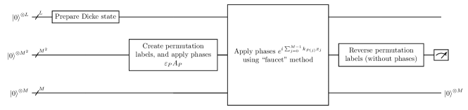
Figure 1: Schematic diagram of the Bethe circuit

This circuit proceeds by the following 5 main steps (see [4] for details):

1. Prepare the system qubits in the so-called Dicke state

   $$\frac{1}{\sqrt{{L\choose M}}}\sum_{0\leq x_{0}<\ldots<x_{M-1}\leq L-1}|x_{0},\ldots,x_{M-1}\rangle\,.$$ (2.9)

2. Prepare the permutation-label qubits in the state

   $$\frac{1}{\sqrt{M!}}\sum_{P}\varepsilon_{P}\,A_{P}|P\rangle\,,$$ (2.10)

   where the states $|P\rangle$ store the permutations by means of “one-hot encoding”.

3. Apply the phases $e^{i\sum_{j=0}^{M-1}k_{P(j)}x_{j}}$ using the “faucet” method. At the end of this step, the faucet qubits return to their original state $|0\rangle^{\otimes M}$.

4. Reverse step 2, except without the phases $\varepsilon_{P}\,A_{P}$.

5. Measure the permutation-label qubits, with success (namely, the system qubits are in a state proportional to the Bethe state (2.4)) on $|0\ldots 0\rangle$.

3 Success probability

We now compute the success probability of the Bethe circuit.

Just prior to the measurements (i.e. at the end of step 4), the Bethe circuit brings the quantum computer to the state

$$|\Psi\rangle=\frac{1}{\sqrt{{L\choose M}}}\frac{1}{M!}|0\ldots 0\rangle|\psi\rangle+\ldots\,,\qquad\langle\Psi|\Psi\rangle=1\,,$$ (3.1)

where $|\psi\rangle$ is the unnormalized state (2.4), and the ellipsis denotes additional terms that are orthogonal to the first. The factor $\frac{1}{\sqrt{{L\choose M}}}$ comes from the operator that creates the Dicke state (2.9) at step 1, and the factor $\frac{1}{M!}=\left(\frac{1}{\sqrt{M!}}\right)^{2}$ comes from the operator that creates the permutation-label state (2.10) and its inverse, see steps 2 and 4 above.

For later convenience, let us define the state $|\phi\rangle$ by the following rescaling of $|\psi\rangle$

$$|\phi\rangle:=\left[\prod_{0\leq j<l\leq M-1}(j,l)\right]|\psi\rangle\,,$$ (3.2)

where we have introduced the notation [8]

$$(j,l):=2-e^{-ik_{j}}-e^{ik_{l}}\,.$$ (3.3)

In terms of this notation, the state (3.1) is given by

$$|\Psi\rangle =\frac{1}{\sqrt{{L\choose M}}}\frac{1}{M!}\frac{1}{\left[\prod_{0\leq j<l\leq M-1}(j,l)\right]}|0\ldots 0\rangle|\phi\rangle+\ldots\,,$$

$$=\alpha|0\ldots 0\rangle|\tilde{\phi}\rangle+\ldots$$ (3.4)

where $|\tilde{\phi}\rangle$ is the normalized state

$$|\tilde{\phi}\rangle:=\frac{|\phi\rangle}{\sqrt{\langle\phi|\phi\rangle}}\,,\qquad\langle\tilde{\phi}|\tilde{\phi}\rangle=1\,,$$ (3.5)

and $\alpha$ is defined by

$$\alpha:=\frac{1}{\sqrt{{L\choose M}}}\frac{1}{M!}\frac{1}{\left[\prod_{0\leq j<l\leq M-1}(j,l)\right]}\sqrt{\langle\phi|\phi\rangle}\,.$$ (3.6)

The probability that all the ancillary qubits are in the state $|0\ldots 0\rangle$, and that the Bethe state $|\tilde{\phi}\rangle$ has therefore been successfully prepared, is $|\alpha|^{2}$. Since all the Bethe roots $\{k_{i}\}$ are real, $(j,l)^{*}=(l,j)$. Hence, the success probability is given by

$$|\alpha|^{2}=\frac{1}{{L\choose M}}\frac{1}{\left(M!\right)^{2}}\frac{1}{\left[\prod_{0\leq j<l\leq M-1}(j,l)(l,j)\right]}\langle\phi|\phi\rangle\,.$$ (3.7)

We observe that the Bethe wavefunction corresponding to the unnormalized state $|\phi\rangle$ (3.2) is normalized in the same way as in [8]. (Indeed, $|\phi\rangle$ also has the form (2.6), but with $A_{I}\neq 1$, and with $A_{P}$ the same (up to an irrelevant phase) as in [8].) The squared norm $\langle\phi|\phi\rangle$ is therefore given by [8]

$$\langle\phi|\phi\rangle=\left[\prod_{0\leq j<l\leq M-1}(j,l)(l,j)\right]\,\det G\,,$$ (3.8)

where $G$ is the so-called Gaudin matrix, which is an $M\times M$ matrix whose components are given by

$$G_{m,n}=\delta_{m,n}\left[L-\sum_{l=0}^{M-1}\frac{4\left(1-\cos k_{l}\right)}{(n,l)\,(l,n)}\right]+\frac{4\left(1-\cos k_{m}\right)}{(n,m)\,(m,n)}\,,\qquad m,n\in\{0,\ldots,M-1\}\,.$$ (3.9)

We conclude from (3.7) and (3.8) that the success probability is given by

$$|\alpha|^{2}=\frac{1}{{L\choose M}}\frac{1}{\left(M!\right)^{2}}\,\det G=\frac{(L-M)!}{L!\,M!}\det G\,.$$ (3.10)

The result (3.10) for the success probability is one of the main results of this paper. Using this formula, we obtain the results in Table 1, which coincide with corresponding results obtained by running the Bethe circuit on the IBM Qiskit statevector simulator.

$L$	$M$	$k_{0},\ldots,k_{M-1}$	$|\alpha|^{2}$
4	2	$\pm 2\pi/3$	0.5
6	2	1.41951, 2.76928	0.463068
6	3	$\pm 1.72277,\pi$	0.157232
8	4	$\pm 1.522,\pm 2.63483$	0.0361418

Table 1: Success probabilities computed using (3.10)

We can now argue that, for a fixed finite number of Bethe roots $M$, the large-$L$ limit of the success probability is given by

$$\lim_{L\rightarrow\infty}|\alpha|^{2}=\frac{1}{M!}\,.$$ (3.11)

Indeed, in view of the relation (3.10), it suffices to show that

$$\lim_{L\rightarrow\infty}\frac{(L-M)!}{L!}\det G=1\,.$$ (3.12)

To this end, we observe that, for large $L$, the Gaudin matrix (3.9) is (up to terms of order 1) proportional to the identity matrix

$$G\sim\mathbb{I}L\qquad\text{ for }\quad L\rightarrow\infty\,,$$ (3.13)

which implies that $\det G\sim L^{M}$ (up to terms of order $L^{M-1}$). Hence,

$$\lim_{L\rightarrow\infty}\frac{(L-M)!}{L!}\det G=\lim_{L\rightarrow\infty}\frac{(L-M)!}{L!}L^{M}=1\,,$$ (3.14)

as claimed.

We checked the result (3.11) by numerically studying the success probability for fixed values of $M$, as a function of $L$. However, for given values of $M$ and $L$, there are generally multiple real solutions of the Bethe equations. For definiteness, we selected the ones with lowest energy (2.8). For brevity, we refer to the corresponding states as “low-energy states”. For the cases $M=1,2,3,4$, we plotted the success probabilities for these low-energy states as a function of $L$, with $L={\rm even}$, as shown in Fig. 2. This data is clearly consistent with the result (3.11).

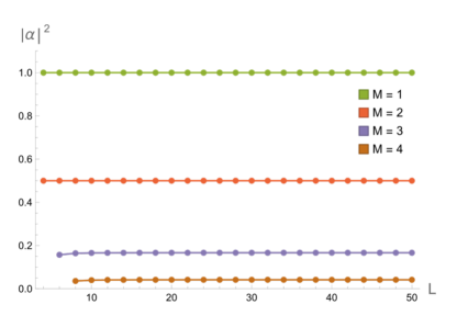
Figure 2: Success probability $|\alpha|^{2}$ for low-energy states with $M=1,2,3,4$ as a function of chain length $L$

The result (3.11) supports the count estimates in [4] of the non-Clifford gates in the Bethe circuit.

4 Correlation functions

For concreteness, we consider here the spin-spin correlation functions

$$\langle\psi_{0}|\sigma^{z}_{0}\,\sigma^{z}_{l}|\psi_{0}\rangle\,,\qquad l=1,2,\ldots,\frac{L}{2}\,,$$ (4.1)

with $L$ even, where $|\psi_{0}\rangle$ is the normalized ground state of the antiferromagnetic Hamiltonian (1.1), which is described by $M=\frac{L}{2}$ real Bethe roots (see e.g. [2, 3]). As already noted in the Introduction, there is an extensive literature on these correlation functions, see e.g. [10, 11, 12, 13, 14, 15, 16, 17, 18, 19, 20, 21, 22, 23, 24] and references therein. Our goal is to determine if – and if so, to what extent – these correlation functions can be computed using a quantum computer.

4.1 Measuring correlators

In order to perform shot-based measurements of the expectation values (4.1) on a quantum computer, we cannot take advantage of built-in functionality (say, in Qiskit) for computing expectation values, since we are preparing the state $|\psi_{0}\rangle$ probabilistically. Nevertheless, as shown below, we can proceed by simply measuring all the qubits, and then appropriately combining the corresponding probabilities, which can be approximated from the corresponding counts.

As a first warm-up exercise, let us consider a quantum computer in the 2-qubit state $|\Psi\rangle$ given by

$$|\Psi\rangle=|0\rangle|a\rangle+|1\rangle|b\rangle\,,\qquad\langle\Psi|\Psi\rangle=\langle a|a\rangle+\langle b|b\rangle=1\,,$$ (4.2)

where $|a\rangle$ and $|b\rangle$ are (unnormalized) 1-qubit states. Suppose that we wish to compute an expectation value in the state $|a\rangle$ (rather than the full state $|\Psi\rangle$), for example, $\langle a|\sigma^{z}|a\rangle/\langle a|a\rangle$. According to the Born rule, upon measuring both qubits of the state $|\Psi\rangle$ in the computational basis, $|\Psi\rangle$ is projected to the computational basis states $|i_{1}\ i_{0}\rangle$ with probabilities

$$p_{i_{1}i_{0}}=|\langle i_{1}\ i_{0}|\Psi\rangle|^{2}\,,\qquad i_{0},i_{1}\in\{0\,,1\}\,,$$ (4.3)

which can be approximated from the corresponding counts. Setting

$$|a\rangle=\sum_{i=0}^{1}a_{i}|i\rangle={a_{0}\choose a_{1}}\,,$$ (4.4)

and similarly for $|b\rangle$, we see that

$$p_{00}=|a_{0}|^{2}\,,\quad p_{01}=|a_{1}|^{2}\,,\quad p_{10}=|b_{0}|^{2}\,,\quad p_{11}=|b_{1}|^{2}\,.$$ (4.5)

We therefore obtain an expression for $\langle a|\sigma^{z}|a\rangle/\langle a|a\rangle$ in terms of probabilities $p_{0i}$

$$\frac{\langle a|\sigma^{z}|a\rangle}{\langle a|a\rangle}=\frac{|a_{0}|^{2}-|a_{1}|^{2}}{|a_{0}|^{2}+|a_{1}|^{2}}=\frac{p_{00}-p_{01}}{p_{00}+p_{01}}\,.$$ (4.6)

As a second warm-up exercise, let us now suppose that the state $|\Psi\rangle$ in Eq. (4.2) is a 3-qubit state, $|a\rangle$ and $|b\rangle$ now being 2-qubit states; and we now wish to compute the 2-qubit expectation value $\langle a|\sigma_{0}^{z}\,\sigma_{1}^{z}|a\rangle/\langle a|a\rangle$. Setting

$$|a\rangle=\sum_{i_{0},i_{1}=0}^{1}a_{i_{1}i_{0}}|i_{1}\ i_{0}\rangle\,,$$ (4.7)

we obtain in a similar way an expression for the desired expectation value in terms of the probabilities $p_{0i_{1}i_{0}}$

$$\frac{\langle a|\sigma_{0}^{z}\,\sigma_{1}^{z}|a\rangle}{\langle a|a\rangle} =\frac{|a_{00}|^{2}-|a_{01}|^{2}-|a_{10}|^{2}+|a_{11}|^{2}}{|a_{00}|^{2}+|a_{01}|^{2}+|a_{10}|^{2}+|a_{11}|^{2}}$$

$$=\frac{p_{000}-p_{001}-p_{010}+p_{011}}{p_{000}+p_{001}+p_{010}+p_{011}}\,.$$ (4.8)

Let us now return to the original problem of evaluating the correlators (4.1). We first use the Bethe circuit to bring the quantum computer to the state (see Eq. (3.4))

$$|\Psi\rangle=\alpha|0\ldots 0\rangle|\psi_{0}\rangle+\ldots\,,$$ (4.9)

and then we simply measure all the qubits. Since the operators $\sigma^{z}_{0}\,\sigma^{z}_{l}$ are diagonal, the expectation values in the state $|\psi_{0}\rangle$ are given in terms of the probabilities $p_{0\ldots 0\,i_{L-1}\ldots i_{0}}$ by

$$\langle\psi_{0}|\sigma^{z}_{0}\,\sigma^{z}_{l}|\psi_{0}\rangle=\frac{\sum_{i_{0},\ldots,i_{L-1}=0}^{1}c^{(l)}_{i_{L-1}\ldots i_{0}}\,p_{0\ldots 0\,i_{L-1}\ldots i_{0}}}{\sum_{i_{0},\ldots,i_{L-1}=0}^{1}p_{0\ldots 0\,i_{L-1}\ldots i_{0}}}\,,$$ (4.10)

where the coefficients $c^{(l)}_{i_{L-1}\ldots i_{0}}$ (with $i_{k}\in\{0\,,1\}$) are either 1 or -1, as in (4.6) and (4.8).

The problem therefore reduces to determining the correct signs $c^{(l)}_{i_{L-1}\ldots i_{0}}$. To this end, let us introduce the diagonal $2^{L}\times 2^{L}$ matrices $D[n]$ whose diagonal elements are either 1 or -1, and which alternate every $n$ elements. As examples, for $L=2$:

$$D[1] =\mathop{\rm diag}\nolimits\left(1,-1,1,-1\right)$$

$$D[2] =\mathop{\rm diag}\nolimits\left(1,1,-1,-1\right)\,.$$ (4.11)

Going here from left to right and starting from 0, the $j^{th}$ diagonal element of $D[n]$ is given by

$$\left(D[n]\right)_{j}=(-1)^{\lfloor\frac{j}{n}\rfloor}\,.$$ (4.12)

We now observe that $\sigma^{z}_{0}=D[1]$, and $\sigma^{z}_{l}=D[2^{l}]$. Hence, the $j^{th}$ diagonal element of the operator whose expectation value we wish to compute is given by

$$\left(\sigma^{z}_{0}\,\sigma^{z}_{l}\right)_{j} =\left(D[1]\right)_{j}\,\left(D[2^{l}]\right)_{j}$$

$$=(-1)^{j}\,(-1)^{\lfloor\frac{j}{2^{l}}\rfloor}\,,$$

$$=:\epsilon^{(l)}[j]\,,\qquad j=0,\ldots,2^{L}-1\,,$$ (4.13)

where the products on the right-hand-side are ordinary products of scalars. We conclude that the coefficients in (4.10) are given by

$$c^{(l)}_{i_{L-1}\ldots i_{0}}=\epsilon^{(l)}[\sum_{k=0}^{L-1}2^{k}i_{k}]\,,$$ (4.14)

where $\epsilon^{(l)}[j]$ is defined in (4.13). As a simple example, for the case $L=2,l=1$, Eqs. (4.10) and (4.14) give (4.8).

4.2 Estimating the number of shots

In order to perform shot-based measurements of the correlators (4.1), how many shots should we use? In order to address this question, we begin by recalling a famous result associated with the Law of Large Numbers (see e.g. [27]): let $\xi_{i}$ be independent, identically distributed random variables, which all have the same expected value ${\rm E}[\xi_{i}]=\mu$ and variance ${\rm Var}[\xi_{i}]=\sigma^{2}$. Then a sample of $n$ such random variables has the average

$$\bar{\xi}=\frac{1}{n}\left(\xi_{1}+\ldots+\xi_{n}\right)\,,$$ (4.15)

and the variance of the sample average is given by

$$\epsilon^{2}:={\rm Var}[\bar{\xi}]=\frac{{\rm Var}[\xi_{i}]}{n}\,.$$ (4.16)

In the usual application to quantum computing, $\xi_{i}$ is regarded as an operator whose expectation value ${\rm E}[\xi_{i}]=\langle\psi|\xi_{i}|\psi\rangle$ is measured by performing (multiple trials of) an experiment consisting of $n$ shots of a quantum circuit that prepares the state $|\psi\rangle$; the result (4.16) then relates the number of shots $n$ to the error $\epsilon$ of the measurement, see e.g. [26].

However, our expectation value (4.1) is with respect to a state $|\psi_{0}\rangle$ that is prepared by the Bethe circuit with probability $|\alpha|^{2}$. Hence, the number of times $n$ that the state $|\psi_{0}\rangle$ is prepared is given by

$$n=N\,|\alpha|^{2}\,,$$ (4.17)

where $N$ is the number of shots of the Bethe circuit. Combining (4.16) and (4.17), we see that the number of shots of the Bethe circuit is given by

$$N=\frac{{\rm Var}[\xi_{i}]}{|\alpha|^{2}\,\epsilon^{2}}\,,$$ (4.18)

where here $\xi_{i}=\sigma^{z}_{0}\,\sigma^{z}_{l}$. We emphasize that $N$ is the number of shots required for the measurement of the full correlation function.

Let us now derive an upper bound on $N$. To this end, we observe that

$${\rm Var}[\xi_{i}] ={\rm E}[\xi_{i}^{2}]-{\rm E}[\xi_{i}]^{2}$$

$$=\langle\psi_{0}|\left(\sigma^{z}_{0}\,\sigma^{z}_{l}\right)^{2}|\psi_{0}\rangle-\left(\langle\psi_{0}|\sigma^{z}_{0}\,\sigma^{z}_{l}|\psi_{0}\rangle\right)^{2}$$

$$=1-\left(\langle\psi_{0}|\sigma^{z}_{0}\,\sigma^{z}_{l}|\psi_{0}\rangle\right)^{2}$$

$$\leq 1\,,$$ (4.19)

where we pass to the third line using the facts $\left(\sigma^{z}_{0}\,\sigma^{z}_{l}\right)^{2}=1$ and $\langle\psi_{0}|\psi_{0}\rangle=1$; and we pass to the last line using the fact $-1\leq\langle\psi_{0}|\sigma^{z}_{0}\,\sigma^{z}_{l}|\psi_{0}\rangle\leq 1$. It then follows from (4.18) that

$$N\leq N_{\rm max}\,,\qquad N_{\rm max}:=\frac{1}{|\alpha|^{2}\,\epsilon^{2}}\,.$$ (4.20)

We note that $N_{\rm max}$ is independent of the value of $l$.

Summarizing: in order to measure the correlations (4.1) within error $\epsilon$, it suffices to perform (multiple trials of) an experiment consisting of $N_{\rm max}$ shots of the Bethe circuit, where $N_{\rm max}$ is given by (4.20), and $|\alpha|^{2}$ is given by (3.10).

4.3 Simulations for small $L$ values

We checked our results (4.10), (4.14) and (4.20) by measuring the spin-spin correlation functions (4.1) using the IBM Qiskit qasm simulator (without noise) for small values of $L$. Specifically, we set $\epsilon=0.01$, and we performed 100 trials (in order to accumulate sufficient statistics to compute mean and standard deviation) of an experiment consisting of $N$ shots of the Bethe circuit, with $N\approx N_{\rm max}$ (4.20), and using (4.10), (4.14) for the measurements. In the experimental (“exp”) columns of Table 2, the values of $|\alpha|^{2}$ and $N$ are noted, and the mean and standard deviation of these 100 trials are reported. We observe that the experimental standard deviations are all within the specified error $\epsilon=0.01$, thereby providing support for (4.20). The theoretical (“th”) columns of Table 2 with $L=4,6,8$ display the values obtained using Mathematica. For comparison, the results for $L=\infty$, which are obtained from the literature, are also displayed.

	$L=4$		$L=6$		$L=8$		$L=\infty$
$l$	th	exp	th	exp	th	exp	th
		$|\alpha|^{2}=0.5$		$|\alpha|^{2}=0.157232$		$|\alpha|^{2}=0.0361418$
		$N=2\times 10^{4}$		$N=6.4\times 10^{4}$		$N=2.8\times 10^{5}$
1	-0.666667	$-0.6657\pm 0.0076$	-0.622839	$-0.6230\pm 0.0072$	-0.608516	$-0.6091\pm 0.0077$	-0.590863 [10]
2	0.333333	$0.3309\pm 0.0090$	0.27735	$0.2777\pm 0.0086$	0.261037	$0.2602\pm 0.0086$	0.242719 [12]
3	–	–	-0.309022	$-0.3102\pm 0.0090$	-0.251937	$-0.2519\pm 0.0088$	-0.200995 [18]
4	–	–	–	–	0.198831	$0.1988\pm 0.0093$	0.138611 [19]

Table 2: The spin-spin correlation functions $\langle\psi_{0}|\sigma^{z}_{0}\,\sigma^{z}_{l}|\psi_{0}\rangle$, where $|\psi_{0}\rangle$ is the normalized ground state of the antiferromagnetic length-$L$ Hamiltonian (1.1)

4.4 Larger $L$ values

As can already be seen from Table 2, as the length $L$ of the chain increases, the number of shots $N$ that are needed to measure the correlators (4.1) to within a specified (fixed) error $\epsilon$ increases. Indeed, the success probability $|\alpha|^{2}$ decreases exponentially with $L$, as expected from (3.11) since $M=L/2$, and as shown in Fig. 3. Correspondingly, there is an exponential increase in $N_{\rm max}$. For example, for the moderate value $L=40$, we find $|\alpha|^{2}\sim 5\times 10^{-20}$, and therefore $N_{\rm max}\sim 2\times 10^{23}$, which is evidently impractical.

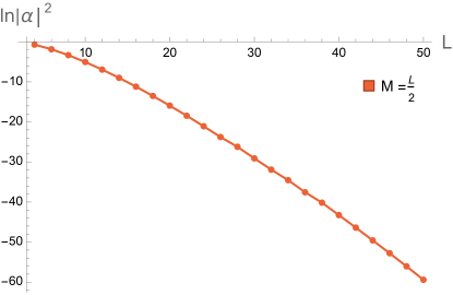
Figure 3: Logarithm of the success probability $\ln|\alpha|^{2}$ for the antiferromagnetic ground state as a function of chain length $L$

As noted in [4], amplitude amplification [28] can generally be used to compensate for low success probability. However, for the problem at hand, the required number of iterations of amplitude amplification would render the circuit impractically deep. Indeed, after just one iteration, the success probability goes up from $\sin^{2}(\theta_{a}):=|\alpha|^{2}$ to $\sin^{2}(3\theta_{a})$ [28]. For $|\alpha|^{2}$ exponentially small, so that $\theta_{a}\approx|\alpha|$, this implies a 9-fold amplification, which is clearly insufficient. The number $m$ of iterations needed to achieve success probability near 1 is given by

$$m=\left\lfloor\frac{\pi}{4\theta_{a}}\right\rfloor\approx\frac{1}{\theta_{a}}\approx\frac{1}{|\alpha|}\,,$$ (4.21)

see Theorem 2 in [28]. For the $L=40$ example considered above, $m\sim 10^{9}$. Since each iteration effectively applies the Bethe circuit twice, the total circuit becomes impractically deep.

5 Discussion

We have found a simple exact formula (3.10) for the probability that the Bethe circuit [4] successfully prepares an eigenstate of the Heisenberg Hamiltonian (1.1) corresponding to real Bethe roots. We have argued that, for large $L$ and fixed number of Bethe roots $M$, the success probability approaches $1/M!$ (3.11). We have also demonstrated the feasibility of using the Bethe circuit to compute the spin-spin correlation functions (4.1) for small values of $L$, see Table 2. However, we see from Fig. 3 that the success probability decreases exponentially with $L$ for the antiferromagnetic ground state (for which $M=L/2$), which precludes the computation of these correlation functions for moderate values of $L$. We have considered here the optimal situation of no noise; of course, the presence of noise would make matters worse.

A contribution to the exponential decrease of the success probability for increasing $M$ comes from the $1/\sqrt{M!}$ factors that are associated with the permutation labels, as noted below (3.1). Since the sum over permutations is an indispensable ingredient of the Bethe wavefunction (2.6), we expect that any probabilistic algorithm for preparing Bethe states will necessarily involve creation of a superposition state of all permutations, such as (2.10); therefore, its success probability will necessarily have those $1/\sqrt{M!}$ factors.

The Bethe algorithm [4], which is for a closed spin chain with periodic boundary conditions, has recently been extended to the case of open spin chains [29]. The latter algorithm is also probabilistic. We expect that the formula for success probability (3.10) can be generalized to the open-chain case. However, the above argument suggests that the success probability for the open chain also decreases rapidly with $M$ (perhaps faster, since there is also a sum over the $2^{M}$ possible reflections), which would imply that – as in the periodic case – the correlation functions (4.1) could be computed only for small values of $L$.

We have considered in Sec. 4 an application of the Bethe circuit involving antiferromagnetic ground states, which have the maximum possible value of $M$ for a given value of $L$ (namely, $M=L/2$), and which correspondingly have the smallest possible success probability. Nevertheless, it could be feasible to prepare states with small values of $M$ – even for moderate values of $L$ – that would not be classically simulable, and which could still have interesting applications [4]. Indeed, as shown in Fig. 2, the success probabilities for small values of $M$ are non-negligible, and are essentially independent of $L$. Such states would correspond to high-energy (low-energy) excited states of the antiferromagnetic (ferromagnetic) Hamiltonian, respectively.

Appendix A Conjectures for estimates of the Gaudin
determinant

We note here some conjectures for bounds on the Gaudin determinant, which arose from our study of the success probability.

The physical requirement $|\alpha|^{2}\leq 1$ together with (3.10) imply the following upper bound on the Gaudin determinant

$$\det G\leq\frac{L!\,M!}{(L-M)!}\,.$$ (A.1)

It would be interesting to find a proof of this result (at least for the class of states considered here, namely, $M\in[1,L/2]$ and $L$ are finite integers with $L$ even, and $k_{0},\ldots,k_{M-1}$ are real and satisfy the Bethe equations) directly from the definition of the Gaudin matrix (3.9). If one could show that the Gaudin matrix is positive (which we have verified for many examples), then the Perron-Frobenius theorem could be used to help show that $\det G\leq L^{M}\leq\frac{L!\,M!}{(L-M)!}$.

From an analysis of many states with real Bethe roots (all such states up to $L=20$, and selected cases up to $L=500$), we find that the success probability for most states satisfies the stronger bound

$$|\alpha|^{2}\leq\frac{1}{M!}\qquad\text{(for most states)}\,,$$ (A.2)

which is compatible with (3.11), and correspondingly

$$\det G\leq\frac{L!}{(L-M)!}\qquad\text{(for most states)}\,.$$ (A.3)

However, we have identified some “exceptional” states that slightly violate these bounds. These exceptional states are all characterized by sets of $M$ equally-spaced “counting numbers”

$$\{-\frac{M-1}{2},-\frac{M-1}{2}+1,\ldots,\frac{M-1}{2}-1\,,\frac{M-1}{2}\}\,,$$ (A.4)

for certain values of $M\geq 3$ and $L\geq 22$, for which $|\alpha|^{2}\,M!=1+\delta$, where $\delta>0$ is of order $10^{-5}$ for $L=22,M=3$, and reaches $10^{-2}$ for $L=500,M=75$. However, consistent with (3.11), we observe that $\delta\rightarrow 0$ for fixed $M$ and sufficiently large $L$.

References

- [1] H. Bethe, “On the theory of metals. 1. Eigenvalues and eigenfunctions for the linear atomic chain,” Z. Phys. 71 (1931) 205–226.
- [2] L. D. Faddeev and L. A. Takhtajan, “Spectrum and scattering of excitations in the one-dimensional isotropic Heisenberg model,” Zap. Nauchn. Semin. 109 (1981) 134–178.
- [3] M. Gaudin, La fonction d’onde de Bethe. Masson, 1983. English translation by J.-S. Caux, The Bethe wavefunction, CUP, 2014.
- [4] J. S. Van Dyke, G. S. Barron, N. J. Mayhall, E. Barnes, and S. E. Economou, “Preparing Bethe Ansatz Eigenstates on a Quantum Computer,” PRX Quantum 2 (2021) 040329, arXiv:2103.13388 [quant-ph].
- [5] A. M. Childs and N. Wiebe, “Hamiltonian simulation using linear combinations of unitary operations,” Quant. Inform. & Comp. 12 (November, 2012) 901, arXiv:1202.5822 [quant-ph].
- [6] D. W. Berry, A. M. Childs, R. Cleve, R. Kothari, and R. D. Somma, “Simulating Hamiltonian Dynamics with a Truncated Taylor Series,” Phys. Rev. Lett. 114 no. 9, (2015) 090502, arXiv:1412.4687 [quant-ph].
- [7] R. I. Nepomechie, “Bethe ansatz on a quantum computer?,” Quant. Inf. & Comp. 21 (2021) 255–265, arXiv:2010.01609 [quant-ph].
- [8] M. Gaudin, B. M. McCoy, and T. T. Wu, “Normalization sum for the Bethe’s hypothesis wave functions of the Heisenberg-Ising chain,” Phys. Rev. D 23 no. 2, (1981) 417.
- [9] V. E. Korepin, “Calculation of norms of Bethe wave functions,” Commun. Math. Phys. 86 (1982) 391–418.
- [10] L. Hulthén, “Über das Austauschproblem eines Kristalles,” Ark. Math. Astron. Fys. 26A (1938) .
- [11] A. Luther and I. Peschel, “Calculation of critical exponents in two-dimensions from quantum field theory in one-dimension,” Phys. Rev. B 12 (1975) 3908–3917.
- [12] M. Takahashi, “Half-filled Hubbard model at low temperature,” J. Phys. C 10 (1977) 1289.
- [13] H. Q. Lin and D. K. Cambell, “Spin-spin correlations in the one-dimensional spin-1/2, antiferromagnetic Heisenberg chain,” J. Applied Phys. 69 (1991) 5947.
- [14] K. A. Hallberg, P. Horsch, and G. Martínez, “Numerical renormalization-group study of the correlation functions of the antiferromagnetic spin-1/2 Heisenberg chain,” Phys. Rev. B 52 no. 2, (1995) R719–R722, arXiv:cond-mat/9505132 [cond-mat].
- [15] N. Kitanine, J. M. Maillet, and V. Terras, “Correlation functions of the XXZ Heisenberg spin- chain in a magnetic field,” Nucl. Phys. B 567 (2000) 554–582, arXiv:math-ph/9907019.
- [16] N. Kitanine, J. M. Maillet, N. A. Slavnov, and V. Terras, “Spin spin correlation functions of the XXZ - 1/2 Heisenberg chain in a magnetic field,” Nucl. Phys. B 641 (2002) 487–518, arXiv:hep-th/0201045.
- [17] S. L. Lukyanov and V. Terras, “Long distance asymptotics of spin spin correlation functions for the XXZ spin chain,” Nucl. Phys. B 654 (2003) 323–356, arXiv:hep-th/0206093.
- [18] K. Sakai, M. Shiroishi, Y. Nishiyama, and M. Takahashi, “Third neighbor correlators of spin 1/2 Heisenberg antiferromagnet,” Phys. Rev. E 67 (2003) 065101, arXiv:cond-mat/0302564.
- [19] H. E. Boos, M. Shiroishi, and M. Takahashi, “First principle approach to correlation functions of spin-1/2 Heisenberg chain: Fourth-neighbor correlators,” Nucl. Phys. B 712 (2005) 573–599, arXiv:hep-th/0410039.
- [20] H. Boos, M. Jimbo, T. Miwa, F. Smirnov, and Y. Takeyama, “Density matrix of a finite sub-chain of the Heisenberg anti-ferromagnet,” Lett. Math. Phys. 75 (2006) 201–208, arXiv:hep-th/0506171.
- [21] V. E. Korepin and O. I. Patu, “XXX spin chain: From Bethe solution to open problems,” PoS SOLVAY (2006) 006, arXiv:cond-mat/0701491.
- [22] J.-S. Caux and J. M. Maillet, “Computation of Dynamical Correlation Functions of Heisenberg Chains in a Magnetic Field,” Phys. Rev. Lett. 95 no. 7, (2005) 077201, arXiv:cond-mat/0502365 [cond-mat.str-el].
- [23] J.-S. Caux, R. Hagemans, and J. M. Maillet, “Computation of dynamical correlation functions of Heisenberg chains: the gapless anisotropic regime,” J. Stat. Mech. 2005 no. 9, (2005) 09003, arXiv:cond-mat/0506698 [cond-mat.str-el].
- [24] J.-S. Caux, “Correlation functions of integrable models: A description of the ABACUS algorithm,” J. Math. Phys. 50 no. 9, (2009) 095214–095214, arXiv:0908.1660 [cond-mat.str-el].
- [25] R. Somma, G. Ortiz, J. E. Gubernatis, E. Knill, and R. Laflamme, “Simulating physical phenomena by quantum networks,” Phys. Rev. A 65 no. 4, (2002) , arXiv:0108146 [quant-ph].
- [26] D. Wecker, M. B. Hastings, N. Wiebe, B. K. Clark, C. Nayak, and M. Troyer, “Solving strongly correlated electron models on a quantum computer,” Phys. Rev. A 92 no. 6, (2015) , arXiv:1506.05135 [quant-ph].
- [27] Wikipedia contributors, “Law of large numbers — Wikipedia, the free encyclopedia.” https://en.wikipedia.org/w/index.php?title=Law_of_large_numbers&oldid=1062022078, 2021. [Online; accessed 27-December-2021].
- [28] G. Brassard, P. Høyer, M. Mosca, and A. Tapp, “Quantum amplitude amplification and estimation,” Quant. Comp. & Inform. (2002) 53–74, arXiv:quant-ph/0005055 [quant-ph].
- [29] J. S. Van Dyke, E. Barnes, S. E. Economou, and R. I. Nepomechie, “Preparing exact eigenstates of the open XXZ chain on a quantum computer,” arXiv:2109.05607 [quant-ph].