Correlations and Critical Behavior
in Lattice Gluodynamics.

Abstract

In the Landau-gauge lattice gluodynamics we find that, both in the SU(2) and SU(3) theory, a correlation of the Polyakov loop with the asymmetry of the $A^{2}$ gluon condensate as well as with the longitudinal propagator makes it possible to determine the critical behavior of these quantities. We discuss finite-volume corrections and reveal that they can be reduced by the use of regression analysis. We also analyze the temperature dependence of low-momenta propagators in different Polyakov-loop sectors.

1 Introduction

In last decades, the deconfinement transition of strong-interacting matter at finite temperature has received considerable theoretical and experimental study. At physical values of the parameters it is a crossover transition, which probably coincides with the chiral transition.

In the limit of infinitely-heavy quarks, the fermion degrees of freedom can be neglected and the crossover transition goes over into the first-order transition in conventional QCD and into the second-order transition in two-color QCD. For this reason, gluodynamics (that is, pure-gauge theory) is widely employed as a testing tool for the studies of the deconfinement transition.

The temperature and volume dependence of the Green’s functions of gauge fields in the vicinity of the critical temperature $T_{c}$ is of particular interest. The critical behavior of the gluon and ghost propagators was considered, in particular, in Fischer:2010fx ; Maas:2011ez ; Aouane:2011fv . In Refs. Oliveira:2014uga ; Silva:2016onh it was found that, close to criticality, the gluon propagator behaves differently in different Polykov-loop sectors.

A interesting example of critical behavior is provided by the chromoelectric-chromomagnetic asymmetry of the dimension-two gluon condensate Chernodub:2008kf . Motivation for the studies of the asymmetry and gluon propagators was also discussed in Aouane:2011fv ; Maas:2011se ; Vercauteren:2010rk and references therein.

Recently, it was demonstrated that correlations between the Polyakov loop and the zero-momentum longitudinal propagator considerably facilitate the analysis of its critical behavior both in the SU(2) Bornyakov:2016geh ; Bornyakov:2018mmf and SU(3) Bornyakov:2021pls gluodynamics. This made it possible to describe critical behavior of the asymmetry and the propagator with unprecendented precision. Here we discuss the assumptions made in Refs.Bornyakov:2016geh ; Bornyakov:2018mmf ; Bornyakov:2021pls and the role of finite-volume effects.

The paper is organized as follows. In the next Section we introduce the definition and describe the details of our numerical simulations. The correlation between the asymmetry ${\cal A}$ and the Polyakov loop ${\cal P}$ forms the subject of Section 3. In Section 4 we consider the finite-volume effects and discuss how the Polyakov loop determined the behavior of the asymmetry and the propagator. The propagators at nonzero momenta are considered in Section 5. In Conclusions we summarize our findings.

2 Designations and lattice settings

We study SU(2) and SU(3) lattice gauge theories with the standard Wilson action in the Landau gauge.

Our calculations are performed on $N_{t}\times N_{s}^{3}$ lattices ($N_{t}=8$, $N_{s}=32,48,72,80$ in the SU(2) case and $N_{t}=8$, $N_{s}=24$ in the SU(3) case). The temperature $T$ is given by $\leavevmode\nobreak\ T=1/aN_{t}\leavevmode\nobreak\$ where $a$ is the lattice spacing; $L=aN_{s}$ is the lattice size. We use the parameter $\displaystyle\tau={T-T_{c}\over T_{c}}$.

In the SU(3) case we employ the scale fixing procedure proposed in Necco:2001xg and use the value of the Sommer parameter $r_{0}=0.5$ fm as in Bornyakov:2011jm . Making use of $\beta_{c}=6.06$ and $\displaystyle{T_{c}\over\sqrt{\sigma}}=0.63$, Ref. Boyd:1996bx gives $T_{c}=294$ MeV and $\sqrt{\sigma}=0.47$ GeV. We study the range of temperatures $0.904T_{c}\leq T\leq 1.104T_{c}$, the corresponding lattice spacings $0.076\leavevmode\nobreak\ \mathrm{fm}\leq a\leq 0.093$ fm. Some $200$ independent Monte Carlo gauge-field configurations are generated for each of the sectors of the Polyakov loop ${\cal P}$ (also referred to as the center sectors):

$$(I)\qquad-\;{\pi\over 3}< \arg{\cal P} <{\pi\over 3}\quad\mbox{referred to as}\quad\mathrm{Re}{\cal P}>0$$ (1)

$$(II)\qquad\quad{\pi\over 3}< \arg{\cal P} <\pi\quad\mbox{referred to as}\quad\mathrm{Re}{\cal P}<0$$

$$(III)\qquad-\;{\pi}< \arg{\cal P} <-\;{\pi\over 3}\;.\quad\mbox{referred to as}\quad\mathrm{Re}{\cal P}<0$$

We make no difference between sectors $II$ and $III$ becuse the quantities under study are independent of $\mathrm{Im}{\cal P}$ as was shown in Bornyakov:2021pls .

In the SU(2) case we use the string tension $\sigma=440$ MeV, which gives Bloch:2002we $T_{c}=297$ MeV. We study the range $0.9987T_{c}\leq T\leq 1.0083T_{c}$, the corresponding lattice spacings $a\approx 0.083$ fm. From 400 to 2200 gauge-field configurations are simulated for each set of the parameters. In the case of SU(2) we make no difference between ${\cal P}$ and $\mathrm{Re}{\cal P}$.

Consecutive configurations are separated by $200\div 400$ sweeps, each sweep includes one local heatbath update followed by $N_{s}/2$ microcanonical updates.

Definitions of the chromo-electric-magnetic asymmetry ${\cal A}$ can be found e.g. in Refs.Chernodub:2008kf ; Bornyakov:2016geh ; the definitions of vector potentials $A_{\mu}(x)$, and the description of gauge-fixing procedure as well as the expressions for the longitudinal $D_{L}(p)$ and transverse $D_{T}(p)$ gluon propagators — in Refs.Bornyakov:2011jm ; Aouane:2011fv ; Bornyakov:2021pls . Here we only present the expression for the asymmetry in terms of the propagators

$${\cal A}={2(N_{c}^{2}-1)N_{t}\over\beta a^{2}N_{s}^{3}}\left[3(D_{L}(0)-D_{T}(0))+\sum_{p\neq 0}\left({3|\vec{p}|^{2}\,-\,p_{4}^{2}\over p^{2}}D_{L}(p)-2D_{T}(p)\right)\right]\;.$$ (2)

Here we do not consider details of the approach to the continuum limit and renormalization considering that the lattices with $N_{t}=8$ (corresponding to spacing $a\simeq 0.08$ fm at $T\sim T_{c}$) are sufficiently fine.

3 Correlations of the longitudinal propagator and the asymmetry with the Polyakov loop

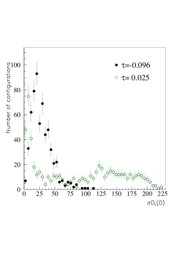
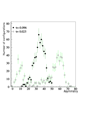
Figure 1: Distributions in the zero-momentum longitudinal propagator (left panel) and the asymmetry (right panel) at $T<T_{c}$ (filled circles) and $T>T_{c}$ (empty circles).

It is convenient to begin the analysis of the critical behavior of the longitudinal $D_{L}(p)$ and transverse $D_{T}(p)$ propagators by considering the temperature dependence of the distributions of gauge-field configurations in $D_{L}(0)$.

First, we observe that the distribution in $D_{L}(0)$ depends strongly on the temperature when $T\sim T_{c}$ (see Fig. 1). This behavior gets even more complicated due to finite-volume effects, which are considered to be substantial at $T\sim T_{c}$.

From the plots in Fig. 1 it is clearly seen that not only the average value but also other quantities characterizing the distribution of confugurations in $D_{L}(0)$ should be thorougly analyzed in order to gain an insight to the critical behavior of the propagators and the asymmetry ${\cal A}$. To characterize the propagator distribution, it is instructive to consider its correlation with the Polyakov loop, whose temperature and volume dependence is well understood Gattringer:2010ms ; Gattringer:2010ug . That is, we use the asymmetry as the reference.

Thus we consider the conditional distribution ${\cal F}\left(\mathbf{D}|{\cal P}\right)$ of $\mathbf{D}=\log\big{[}\sigma D_{L,T}(0)]$ at a particular value of the Polyakov loop ${\cal P}$ and perform regression analysis based on the linear regession model

$$\langle\mathbf{D}(\tau)\rangle_{\cal P}\simeq{\cal D}_{0}^{\!(L,T)}(\tau)+{\cal D}_{1}^{\!(L,T)}(\tau)\operatorname{Re}{\cal P}(\tau)+{\cal D}_{2}^{\!(L,T)}(\tau)\big{(}\operatorname{Re}{\cal P}(\tau)\big{)}^{2}\;,$$ (3)

where $\langle\mathbf{D}(\tau)\rangle_{\cal P}$ is the conditional average of the logarithm of the respective normalized propagator at a given value of the Polyakov loop ${\cal P}$. The results for the longitudinal propagator are shown in Fig. 2.

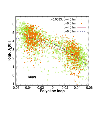
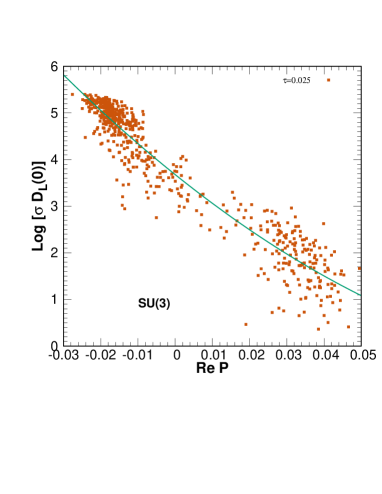
Figure 2: Scatter plots illustrating correlation between the zero-momentum longitudinal propagator and the Polyakov loop. On the left panel data are shown at two different volumes and the same temperature. Shown lines are the regression curves based on the linear model (3).

A similar procedure is performed for the asymmetry,

$$\langle{\cal A}\rangle_{\cal P}\simeq{\cal A}_{0}(\tau)+{\cal A}_{1}(\tau)\operatorname{Re}{\cal P}(\tau)+{\cal A}_{2}(\tau)\big{(}\operatorname{Re}{\cal P(\tau)}\big{)}^{2}\,,$$ (4)

where the parameters ${\cal A}_{0}$, ${\cal A}_{1}$, and ${\cal A}_{2}$ are also determined from the fit to data. The results are shown in Fig. 3.

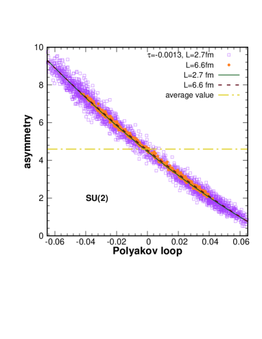
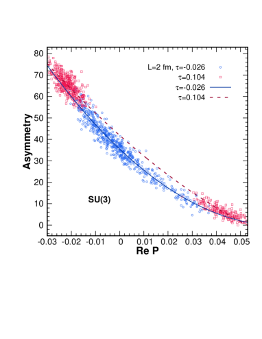
Figure 3: Scatter plots illustrating correlation between the asymmetry and the Polyakov loop. Data are shown at two different lattice sizes and the same temperature in the SU(2) case (left panel) and at two different temperatures and the same lattice size in the SU(3) case (right panel). Shown lines are the regression curves based on the linear model (4).

4 Finite-volume effects and properties of the correlations

The right-hand side of the formula (4) is useful for an evaluation of the average value of the asymmetry in the infinite-volume limit at the temprature $\tau$, where ${\cal P}(\tau)$ is the respective infinite-volume value of the Polyakov loop. Firstly, the sample average value of the asymmetry in the infinite-volume limit coincides with the conditional average at ${\cal P}(\tau)$ because the variance of the Polyakov-loop distribution tends to zero as $L\to\infty$. Secondly, finite-volume effects for the predicted value (4) are much less than the sample average as is shown in Fig. 4. Infinite-volume extrapolation of the results shown on the right panel must coincide with those on the left panel. Thus a comparison of panels illustrates huge finite-volume effects due to an exclusion of one center sector, which is common practice at $0<\tau<\!\!\!1$. The left panel illustrates that the regression analysis gives much better precision for the finite-volume expectation values of the asymmetry than the conventional use of the sample average. It is also seen that an inclusion of both center sectors results not only in substantial decrease of the finite-volume effects, but also in some decrease of precision.

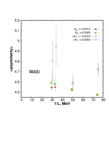
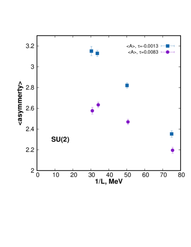
Figure 4: Finite-volume effects for the asymmetry, ${\cal A}_{0}$ $\langle{\cal A}\rangle$ is the sample average. Left panel: both center sectors are taken into consideration. Right panel: results for the sector ${\cal P}>0$.

It is seen on the left panel of Fig. 3 that its correlation with ${\cal P}$ becomes more pronounced with an increase of the volume. To study the dependence of the correlation on the volume, we use the Fraction of Variance Unexplained (FVU) designated by $S$ as a measure of the degree of correlation. It represents the ratio of the variance of the residuals $e_{A}(n)={\cal A}_{n}-{\cal A}_{0}-{\cal A}_{1}\operatorname{Re}{\cal P}_{n}-{\cal A}_{2}(\operatorname{Re}{\cal P}_{n})^{2}$ and the sample variance $M_{2}({\cal A})$,

$$S={Q\over M_{2}({\cal A})},\quad\mbox{where}\quad Q=\sum_{n=1}^{N_{data}}e^{2}_{A}(n)\,,\quad M_{2}({\cal A})=\sum_{n=1}^{N_{data}}|{\cal A}_{n}-\langle{\cal A}\rangle|^{2}\,.$$ (5)

In the general case, $0\leq S\leq 1$; $S=0$ implies that the asymmetry is nothing but a function of the Polyakov loop; $S=1$ means that they are independent of each other. The results are shown in Fig. 5. A similar estimate of $S$ is performed also for the propagator.

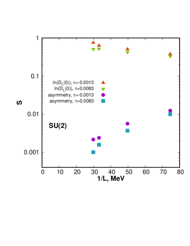
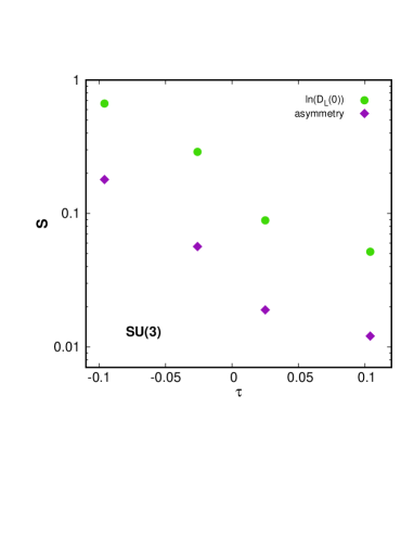
Figure 5: Fraction of variance unexplained: the dependence on lattice size is shown in the SU(2) case (left panel), the dependence on the temperature – for the SU(3) case (right panel) both for ${\cal A}$ and $\mathbf{D}$

We see that the FVU for the asymmetry tends to zero as $L\to\infty$, whereas for the propagator it remains on the order of unity. The temperature dependence of FVU is explained by taking all center sectors into account at $T>T_{c}$ providing a wide range of Polyakov-loop variation. We take all center sectors into consideration because in a finite volume transitions between them are not negligible even at $T>T_{c}$ when $\tau<\!\!\!<1$.

Our data give some evidence that, in the infinite-volume limit, the zero-momentum longitudinal propagator is not a proper function of the Polyakov loop, it remains a random variable correlated with the Polyakov loop, whereas the asymmetry becomes a proper function of the Polyakov loop.

Nevertheless, our conclusion of the critical behavior of the propagator presenrted in Refs.Bornyakov:2016geh ; Bornyakov:2018mmf ; Bornyakov:2021pls holds true because it is based on the assumption of the smooth dependence of the conditional average $\langle\mathbf{D}(\tau)\rangle_{\cal P}$ on ${\cal P}$, no assumptions on its variance are made. Therewith, the regression curve can be extracted from the data only with a limited precision, therefore, the concept of smoothness should be formulated for the corridor of errors rather than for the proper function.

In this context, smoothness of the regression function $f({\cal P})\equiv\langle\mathbf{D}(\tau)\rangle_{\cal P}$ at ${\cal P}={\cal P}_{s}$ means that the value $f({\cal P}_{s})$ as well as the derivative $\displaystyle{df({\cal P})\over d{\cal P}}\Big{|}_{{\cal P}={\cal P}_{s}}$ evaluated over the range ${\cal P}<{\cal P}_{s}$ coincide within statistical error with those evaluated over the range ${\cal P}>{\cal P}_{s}$. It should be emphasized that our conclusions on the critical behavior are based on smothness at ${\cal P}_{s}=0$.

Our data fulfil this criterion. For example, if we take ${\cal P}_{s}=0$ and the SU(3) data for $\tau=-0.096$ so that the data come close to ${\cal P}_{s}$, then we can use the fit function

$$\langle{\cal A}\rangle_{\cal P}\simeq{\cal A}_{0}+{\cal A}_{1}\operatorname{Re}{\cal P}$$ (6)

both at ${\cal P}<{\cal P}_{s}$ and at ${\cal P}>{\cal P}_{s}$; to put it differently, the third term in formula (4) can be omitted because ${\cal P}$ varies over a small range. In so doing, we arrive at

$${\cal A}_{0}=33.91(85),\quad{\cal A}_{1}=-966(16) \quad{\cal P}<0$$ (7)

$${\cal A}_{0}=33.90(64),\quad{\cal A}_{1}=-962(91) \quad{\cal P}>0\ .$$

However, the assumption of smooth dependence should be tested on a larger statistics, for which a reliable extrapolation to the point ${\cal P}_{s}=0$ is possible both from the domain ${\cal P}<0$ and ${\cal P}>0$ when $\tau>0$.

Smooth dependence of the conditional averages $\langle{\cal A}\rangle_{\cal P}$ and $\langle\mathbf{D}\rangle_{\cal P}$ on ${\cal P}$ at ${\cal P}=0$ implies that these quantities and, therefore, the infinte-volume limits of the respective sample averages considered as the functions of $T$ have the same singularity/nonanalyticity at $T=T_{c}$ that the Polyakov loop.

5 Propagators at nonzero momenta

The mentioned test on smoothness can also be motivated by our observation that the temperature dependence of the longitudinal propagator at nonzero momenta differs significantly from that at zero momentum, which is shown in Fig. 6. It is clearly seen that the temperature dependence of the zero-momentum propagator is in a good agreement with that found in Refs. Oliveira:2014uga ; Silva:2016onh .

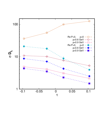
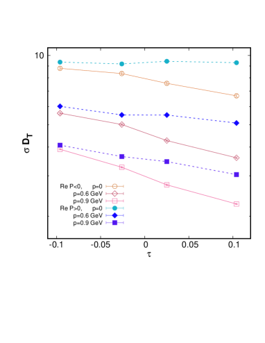
Figure 6: Temperature dependence of the longitudinal (left panel) and transverse (right panel) gluon propagators at various values of momenta in the SU(3) case. Lines are shown just to guide the eye, also notice the logarithmic scale on the ordinate axis.

However, we find that the zero-momentum longitudinal gluon propagator decreases with the temperature in the sector $\mathrm{Re}{\cal P}>0$ and rapidly increases in the sectors $\mathrm{Re}{\cal P}<0$, whereas longitudinal gluon propagator at $p\sim 0.5\div 1$ GeV decreases with temperature in all Polyakov-loop sectors. Thus a sharp peak of the longitudinal gluon propagator in the sectors $\mathrm{Re}{\cal P}<0$ appears in the deep infrared at $T\sim T_{c}$. Physical interpretation of such peak may be as follows: a formation of a large bubble of the phase with $\mathrm{Re}{\cal P}<0$ in gluon matter at $T>T_{c}$ in the phase with $\mathrm{Re}{\cal P}>0$ gives rise to huge fluctuations of chromoelectric fields which should emerge when the size of such bubble exceeds the scale determined by the width of the above-mentioned peak.

Temperature dependence of the transverse propagator at nonzero momenta is shown in the right panel of Fig. 6. It is interesting to remark that it substantially decreases with temperature in the sector $\mathrm{Re}{\cal P}$. However, this observation calls for further investigation.

6 Conclusions

We have studied numerically the asymmetry and the longitudinal gluon propagator in the Landau-gauge SU(2) and SU(3) gluodynamics close to criticality. Our findings can be summarized as follows:

• The correlations between ${\cal A}$ and ${\cal P}$ between $\mathbf{D}$ and ${\cal P}$ indicate that the conditional averages $\langle{\cal A}\rangle_{\cal P}$ and $\langle\mathbf{D}\rangle_{\cal P}$ are smooth functions of ${\cal P}$ at ${\cal P}=0$.

• In the infinite-volume limit, the asymmetry is completely determined by the Polyakov loop, whereas the propagators are only partially determined (that is, the gluon propagator at a given value of ${\cal P}$ represents a random variable even in the infinite-volume limit. )

• The use of regression analysis substantially reduces finite-volume effects.

• Finite-volume effects in different center sectors partially cancel each other.

• The temperature dependence of the longitudinal gluon propagator at $p<1$ GeV and $T\sim T_{c}$ in the Polyakov-loop sectors with $\mathrm{Re}{\cal P}<0$ is qualitatively different at $p=0$ and $p=p_{min}\sim 600$ MeV.

Acknowledgments. Computer simulations were performed on the IHEP (Protvino) Central Linux Cluster and ITEP(Moscow) Linux Cluster. This work was supported in part by the Russian Foundation for Basic Research, grant no.20-02-00737 A.

References

- (1) C.S. Fischer, A. Maas, J.A. Muller, Eur.Phys.J. C68, 165 (2010), 1003.1960
- (2) A. Maas, J.M. Pawlowski, L. von Smekal, D. Spielmann, Phys. Rev. D85, 034037 (2012), 1110.6340
- (3) R. Aouane, V. Bornyakov, E. Ilgenfritz, V. Mitrjushkin, M. Muller-Preussker et al., Phys.Rev. D85, 034501 (2012), 1108.1735
- (4) O. Oliveira, P.J. Silva, PoS LATTICE2014, 355 (2014), 1411.0133
- (5) P.J. Silva, O. Oliveira, Phys. Rev. D 93, 114509 (2016), 1601.01594
- (6) M.N. Chernodub, E.M. Ilgenfritz, Phys. Rev. D78, 034036 (2008), 0805.3714
- (7) A. Maas, Phys. Rept. 524, 203 (2013), 1106.3942
- (8) D. Vercauteren, H. Verschelde, Phys. Rev. D82, 085026 (2010), 1007.2789
- (9) V.G. Bornyakov, V.K. Mitrjushkin, R.N. Rogalyov, Phys. Rev. D 100, 094505 (2019), 1609.05145
- (10) V. Bornyakov, V. Bryzgalov, V. Mitrjushkin, R. Rogalyov, Int. J. Mod. Phys. A 33, 1850151 (2018), 1801.02584
- (11) V.G. Bornyakov, V.A. Goy, V.K. Mitrjushkin, R.N. Rogalyov, Phys. Rev. D 104, 074508 (2021), 2101.03605
- (12) S. Necco, R. Sommer, Nucl. Phys. B 622, 328 (2002), hep-lat/0108008
- (13) V.G. Bornyakov, V.K. Mitrjushkin (2011), 1103.0442
- (14) G. Boyd, J. Engels, F. Karsch, E. Laermann, C. Legeland, M. Lutgemeier, B. Petersson, Nucl. Phys. B 469, 419 (1996), hep-lat/9602007
- (15) J.C.R. Bloch, A. Cucchieri, K. Langfeld, T. Mendes, Nucl. Phys. B Proc. Suppl. 119, 736 (2003), hep-lat/0209040
- (16) C. Gattringer, Phys. Lett. B 690, 179 (2010), 1004.2200
- (17) C. Gattringer, A. Schmidt, JHEP 01, 051 (2011), 1011.2329