Internal Gravity Waves in the Earth’s Ionosphere

Abstract

The theory of low-frequency internal gravity waves (IGWs) is readdressed in the stable stratified weakly ionized Earth’s ionosphere. The formation of dipolar vortex structures and their dynamical evolution, as well as, the emergence of chaos in the wave-wave interactions are studied both in presence and absence of the Pedersen conductivity. The latter is shown to inhibit the formation of solitary vortices and the onset of chaos.

I Introduction

Internal gravity waves (IGWs) are omnipresent in the atmosphere and ocean, and are the low frequency counterparts of known acoustic-gravity waves (AGWs). Such waves appear in the interior of a stratified conducting fluid and are stimulated by the buoyancy providing the restoring force which opposes the vertical displacements of atmospheric particles under gravity. The typical horizontal scale for these waves range from $10$ to $1000$ km and their intrinsic frequencies $(\omega)$ vary in between the Coriolis parameter $f=2\Omega\sin\lambda$ (where $\Omega$ is the angular velocity of the planet and $\lambda$ the latitude) and the Brunt-Väisälä frequency $\omega_{g}$ i.e., in the interval $10^{-4}$ s${}^{-1}<\omega<1.7\times\times 10^{-2}$ s^-1 [1, 2, 3, 4, 5]. The IGWs play crucial roles in the transportation of charged particles as well as transfer of momentum and energy as they propagate vertically in the regions starting from the Earth’s surface to the upper atmosphere and ionosphere. Furthermore, the IGWs can have relevance in the forcast problem of earthquakes and the generation of large scale zonal flows [6], the formation of solitary vortices [7], as well as chaos [8, 9] and turbulence [10, 11] in the Earth’s atmosphere.

A number of fascinating phenomena can occur when the Coriolis force due to the Earth’s rotation comes into the picture. It has been established that such force not only manifests the coupling of high frequency AGWs and the low frequency IGWs, but also significantly alters the resonance and cut-off frequencies [12, 13]. Furthermore, in ionospheric layers the Ampére force due to the interaction of the induced ionospheric currents with the geomagnetic field can have strong influence on the dynamics of ionospheric charged particles. It has been shown that such force can lead to the wave damping and the damping rate is proportional to the Pedersen conductivity associated with it [12, 13].

Recently, a number of researchers have focused their attention to investigate the dynamics of IGWs in different contexts. To mention a few, Bulatov et al. [14] have shown that the IGWs can be generated far from a non-local source of disturbances in a layer of stratified media of a finite depth. The theory of AGWs was revisited by Chatterjee et al. [11] to study the nonlinear coupling of AGWs and IGWs by taking into account the effects of the Coriolis force both in the contexts of the Zakharov approach [15] and the wave kinetic theory approach [16, 17]. Pati et al. [9] studied the multistable dynamics of nonlinear AGWs in ionospheric rotating fluids by the influence of the Coriolis force. They have shown that the AGWs can evolve into periodic and chaotic states. Similar chaotic dynamics of AGWs but in a different context (without the effect of the Coriolis force) was reported by Roy et al. [8]. On the other hand, the propagation characteristics of electromagnetic IGWs have been studied by Kaladze et al. [18, 19] in an ideally conducting incompressible medium in presence of a constant magnetic field. It has been shown that the IGWs can couple even with Alfvén waves.

In this paper, we consider the nonlinear dynamics of IGWs in the weakly ionized Earth’s ionosphere embedded in the constant geomagnetic field (at sufficiently high latitudes) and study the evolution of solitary vortices with different space localization as well as the existence of chaos in a low dimensional model. The effects of the Ampére force on the dynamical evolution of IGWs are demonstrated. It is shown that the Pedersen conductivity associated with the electrmagnetic force dissipates the wave energy thereby inhibiting the formation of a vortex structure with finite wave energy and the occurrence of chaos in the wave-wave interactions. The manuscript is organized as follows. In Sec. II, the theoretical model along with the physical assumptions for the description of IGWs are discussed. The formation of dipolar vortex and the evolution of chaos are also demonstrated in two subsections II-A and II-B. Finally, results are concluded in Sec. III.

II Theoretical formulation and nonlinear dynamics of IGWs

We consider the nonlinear dynamics and evolution of low-frequency IGWs in the Earth’s ionosphere. Specifically, we focus on the dynamics of IGWs that are generated at high latitudes in the northern hemisphere in which the constant geomagnetic field is vertically downwards along the $z$-axis (increasing upward), i.e., $\mathbf{B}_{0}=-B_{0}\hat{z}$. The other two ($x$ and $y$) axes are assumed to be directed from the west to the east and from the south to the north directions. Furthermore, at high latitudes the Earth’s angular velocity can have only a vertical component, i.e., $\mathbf{\Omega}=(0,0,\Omega_{0})$. In the non-inductive approximation, one can consider only the current $\mathbf{j}$ that originates in the medium due to the flow of electrons and ions, and the action of the geomagnetic field on them imposes us to consider the Ampére $(\mathbf{j}\times\mathbf{B}_{0})$ force on the dynamics of charged particles. Thus, typical forces that can influence the dynamics of ionospheric plasmas are namely, the pressure gradient force, the Ampére force, the Coriolis force and the gravitational force. However, depending on the regions of the Earth’s atmosphere we consider, different forces can become dominant over the other(s). For example, in the $E$-layer with $n/N\sim 10^{-8}-10^{-6},~{}B_{0}\sim 0.6\times 10^{-4}~{}\mathrm{T}$, $\nu_{ei}\sim\nu_{in}\sim 10^{3}~{}\mathrm{s}^{-1},~{}\nu_{en}\sim 10^{4}~{}\mathrm{s}^{-1}$ and $\sigma_{H}\sim 3\times 10^{-4}~{}\mathrm{S/m}$, both the Ampére force and the Coriolis force can have significant impact on the charged particles, whereas in the $D$ and $E$ layers, one can safely neglect the contributions of the Ampére force and the Coriolis force respectively [12, 13]. Here, $n/N$ is the ratio between the equilibrium number densities of electrons or ions and neutrals, $B_{0}$ is the static magnetic field, and $\nu_{ei},~{}\nu_{en}$ and $\nu_{in}$, respectively, denote the effective electron-ion, electron-neutral and ion-neutral collisional frequencies.

As a starting point, we disregard any influence of the Ampére force and the Coriolis force. Thus, in stratified weakly ionized quasi-neutral ionospheric plasma layers, the dynamics of charged particles can be described by the following continuity equation, momentum balance equation and the equation of state.

$$\frac{\partial\rho}{\partial t}+\nabla\cdot(\rho\mathbf{v})=0,$$ (1)

$$\rho\frac{d\mathbf{v}}{dt}=-\nabla p+\rho\mathbf{g},$$ (2)

$$\frac{d}{dt}\left(p-c_{s}^{2}\rho\right)=0,$$ (3)

where $d/dt=\partial/\partial t+\mathbf{v}\cdot\nabla$, $\mathbf{v}$ is the fluid flow velocity in a uniform gravity field with acceleration $\mathbf{g}=(0,0,-g)$, $p$ $(\rho)$ is the fluid pressure (mass density), and $c_{s}$ is the acoustic speed. In quasi-neutral plasmas, we have neglected the inner electrostatic field and the vortex component of the self-generated electromagnetic field [12, 13]. The background (unperturbed by waves) pressure $p_{0}$ and the mass density $\rho_{0}$, stratified by the gravitational field, are given by the hydrostatic equilibrium equation $dp_{0}(z)/dz=-\rho_{0}(z)g$ with $p_{0}(z)=c_{s}^{2}\rho_{0}(z)$ which gives $\rho_{0}(z)=\rho_{0}(0)\exp(-z/H)$ and $p_{0}(z)=p_{0}(0)\exp(-z/H)$, where $H=c_{s}^{2}/g$ is the density scale height of the atmosphere.

In what follows, we obtain a set of nonlinear equations for the evolution of IGWs. We note that the density variation $(\rho_{1})$ by the IGWs scales as $\rho_{1}/\rho_{0}\sim(1-4)\times 10^{-2}$, so that in the momentum equation (2) one can approximate $\rho d\mathbf{v}/dt$ as $\rho_{0}(z)d\mathbf{v}/dt$ (Boussinesq approximation). Furthermore, using the incompressibility condition $\nabla\cdot\mathbf{v}=0$ the two-dimensional evolution equations for IGWs in the $xz$-plane with $\mathbf{v}=(u,0,w)$ can be obtained as [7, 20]

$$\frac{\partial}{\partial t}\left(\Delta\psi-\frac{\psi}{4H^{2}}\right)+J(\psi,\Delta\psi)=-\frac{\partial\chi}{\partial x},$$ (4)

$$\frac{\partial\chi}{\partial t}+J(\psi,\chi)=\omega_{g}^{2}\frac{\partial\psi}{\partial x},$$ (5)

where $\psi(x,z)$ is the velocity stream function, given by, $u=-{\partial\psi}/{\partial z},~{}w={\partial\psi}/{\partial x}$; $\chi(x,z)=g\rho_{1}/\rho_{0}(0)$ is the variable associated with the density perturbation $\rho_{1}$, $\omega_{g}=\sqrt{g/H}$ is the Brunt-Väisälä (buoyancy) frequency for the incompressible fluid, $\Delta={\partial^{2}}/{\partial x^{2}}+{\partial^{2}}/{\partial z^{2}}$ is the two-dimensional Laplacian, and $J(a,b)=({\partial a}/{\partial x})({\partial b}/{\partial z})-({\partial a}/{\partial z})({\partial b}/{\partial x})$ is the Jacobian.

From (4) and (5) we note that the total wave energy is conserved, i.e., $\partial{\cal E}/\partial t=0$, implying that a steady state solution can exist, where the energy ${\cal E}$ is given by

$${\cal E}=\int\int\left[\frac{1}{2}\left(\nabla\psi\right)^{2}+\frac{1}{8}\frac{\psi^{2}}{H^{2}}+\frac{1}{2}\frac{\chi^{2}}{\omega_{g}^{2}}\right]dxdz.$$ (6)

Before going into the nonlinear evolution of IGWs, it is pertinent to obtain the linear dispersion relation in the limit of small amplitude waves with frequency $\omega$ and the wave vector $\mathbf{k}=(k_{x},k_{z})$. Thus, we have

$$\omega^{2}=\frac{k_{x}^{2}\omega_{g}^{2}}{k^{2}+1/4H^{2}},$$ (7)

where $k^{2}=k_{x}^{2}+k_{z}^{2}$. From (7) it can be assessed that the wave frequency varies in the regime $10^{-4}$ s${}^{-1}<\omega~{}(\lesssim\omega_{g})<1.7\times 10^{-2}$ s^-1 and the wavelength $k^{-1}\sim H\sim(5-10)$ Km. Also, the phase velocity $|v_{\text{ph}}|\equiv|\omega/k_{x}|\leq v_{\text{ph}}^{\text{max}}\sim 2H\omega_{g}=2\sqrt{gH}$. Typically, at a reduced atmospheric height with $H\sim 6$ Km so that $H\omega_{g}\sim 250$ m/s, we have $v_{\text{ph}}\sim v_{g}\sim v_{\text{ph}}^{\text{max}}\sim 500$ m/s, where $v_{g}$ denotes the group velocity. These estimates agree with some existing observations [21]. So, a source of charged particles moving along the $x$-direction with a velocity larger than $v_{\text{ph}}^{\text{max}}$ can not resonantly interact with the IGWs and hence no energy loss of the wave. In this case, one can look for a stationary solution of IGWs, i.e., the localization of a pulse in a frame moving with a speed $|U|>v_{\text{ph}}^{\text{max}}$ along the $x$-axis. Such nonlinear solitary structures are supersonic and their amplitudes do not decay with time due to the generation of the linear wave mode with $|v_{\text{ph}}|\leq v_{\text{ph}}^{\text{max}}$. Furthermore, we are interested in the frequency regime which is much higher than that due to the Coriolis acceleration, i.e., $\partial/\partial t\gg f$, where $f=2\Omega\sin\lambda\sim 7\times 10^{-5}~{}\mathrm{rad/s}$ with $\lambda$ denoting the latitude.

Nevertheless, the appearance of the nonlinear Jacobian terms in (4) and (5) open up many possibilities to investigate. For examples, they can give rise the formation of various coherent localized vortex structures [22] and the onset of chaos in the coupling of different wave modes [8]. However, the scenario changes significantly when the influence of the Ampére force enters the dynamics of IGWs. In this case, the equation of motion (2) changes to

$$\rho\frac{d\mathbf{v}}{dt}=-\nabla p+\mathbf{j}\times\mathbf{B}_{0}+\rho\mathbf{g},$$ (8)

where the current $j$ is given by the reduced form of the generalized Ohm’s law [12]

$$\mathbf{j}=\sigma_{\perp}\mathbf{E}_{d\perp}+\frac{\sigma_{H}}{B_{0}}\mathbf{B}_{0}\times\mathbf{E}_{d},$$ (9)

in which only the dynamo field $\mathbf{E}_{d}=\mathbf{u}\times\mathbf{B}_{0}$ contributes to the electric field. Also, in (9), the suffix $\perp$ denotes the components perpendicular to the constant magnetic field; $\sigma_{\perp}\equiv\sigma_{p}$ and $\sigma_{H}$ are, respectively, the perpendicular (Pedersen) and Hall conductivities. The inclusion of this new force leads to a modification of (4), i.e.,

$$\frac{\partial}{\partial t}\left(\Delta\psi-\frac{\psi}{4H^{2}}\right) +J(\psi,\Delta\psi)=-\frac{\partial\chi}{\partial x},$$

$$-\frac{\sigma_{p}B_{0}^{2}}{\rho_{0}}\left(\frac{\partial^{2}\psi}{\partial z^{2}}-\frac{\psi}{4H^{2}}\right)$$ (10)

such that the coupled equations (5) and (10) describe the nonlinear dynamics of low-frequency IGWs with the effects of the magnetic viscosity $(\eta_{0}=\sigma_{p}B_{0}^{2}/\rho_{0})$. The latter, however, violates the conservation of wave energy since the energy equation changes to

$$\frac{\partial{\cal E}}{\partial t}+\eta_{0}\int\int\left[\left(\frac{\partial\psi}{\partial z}\right)^{2}+\frac{1}{4}\frac{\psi^{2}}{H^{2}}\right]dxdz=0,$$ (11)

i.e., $\partial{\cal E}/\partial t\leq 0$ for $\eta_{0}>0$ implying that a steady state solution with finite wave energy does not exist, i.e., the IGW gets damped by the effect of $\eta_{0}$. The linear damping rate can be obtained as

$$\gamma=-\frac{1}{2}\eta_{0}\frac{k_{z}^{2}+1/4H^{2}}{k^{2}+1/4H^{2}}.$$ (12)

From (12) it is evident that the damping rate increases with increasing values of the magnetic field. For a set of parameters as in the Earth’s $F$ layer, its value can be estimated as $|\gamma|\sim\eta_{0}\sim 10^{-4}$ s^-1, i.e., the damping rate is relatively small compared to the IGW frequency $\omega\sim 10^{-2}~{}\mathrm{s}^{-1}$. It follows that the linear IGWs can develop into a certain nonlinear stage (before it being dissipated) to form vortex structures whose evolution is governed by (5) and (10). In the following two subsections II-A and II-B we will investigate (4), (5), and (10) in more details, and look for stationary vortex solutions together with their dynamical evolution as well as the occurrence of chaos in low dimensional models.

II-A Formation of dipolar vortex

In a stationary frame $\xi=x-Ut$ and $z=z$ moving with a velocity $U$ along the $x$-axis, Shukla [22] obtained from a set of equations similar to (4) and (5) with $\eta_{0}=0$ a class of solutions including chains of vortices and circular vortex with monotonic profile as well as dipolar vortex. Following [22] another undamped dipolar vortex solution of (4) and (5), which is regular at the center and which vanishes at infinity, can be obtained for $\eta_{0}=0$ by applying the transformations $\xi=x-Ut$ and $z=z$, and considering the linear relation between $\psi$ and $\chi$: $\chi=-(\omega_{g}^{2}/U)\psi$ as

$$\psi(r,\phi)=aUF(r)\cos\phi,$$ (13)

where

$$F(r)=\left\{\begin{array}[]{cc}\frac{p^{2}}{k^{2}}\frac{J_{1}(kr)}{J_{1}(ka)}-\frac{(p^{2}+k^{2})r}{ak^{2}},&(r<a)\\ -\frac{K_{1}(pr)}{K_{1}(pa)},&(r\geq a).\end{array}\right.$$ (14)

Here, $\xi=r\sin\phi,~{}z=r\cos\phi$, $a$ is the vortex radius, $p^{2}=(1/4H^{2})-{\omega_{g}^{2}}/{U^{2}}>0$, and $J_{n}$ $(K_{n})$ is the Bessel function of first kind (the McDonald function) of order $n$. The vortex solution (13) is antisymmetric with respect to $z$ and the vorticity $\zeta=-\Delta\psi$ is continuous at $r=a$. Also, since $p^{2}>0$, the vortex profile can propagate along the $x$-axis with the supersonic velocity $|U|>v^{\text{max}}_{\text{ph}}$ without any resonance with the linear wave. The typical size of the vortex $a$ can be estimated as

$$a\sim p^{-1}=\frac{2H|U|}{\left(U^{2}-4H^{2}\omega_{g}^{2}\right)^{1/2}}\approx 2H.$$ (15)

Thus, the vortex structure of IGWs (with size $a\sim 2H\sim 15$ Km), which is exponentially localized in space and is regular at the center, can propagate in east-west directions (i.e., along $x$-axis) with the supersonic velocity $U$ and inevitably preventing the generation of linear modes by the moving structure (as the linear wave speed is $v_{\text{ph}}\lesssim v^{\text{max}}_{\text{ph}}$).

Another class of vortex solution of Eqs. (4) and (5) can be obtained by considering $\chi=-\omega_{g}H\Delta\psi$. For the phase velocity $U<0$ one obtains

$$\psi=AJ_{1}(kr)\cos\phi,$$ (16)

where $A$ is a constant and $k^{2}=(1/H^{2})\left(1-{U}/{v^{\text{max}}_{\text{ph}}}\right)>0$. We note that the dipole vortex solution (16) is regular at the center $r=0$ and its amplitude $(\propto 1/\sqrt{kr})$ vanishes at infinity. The size of the vortex can be estimated as $a\sim k^{-1}\sim H\sim 10$ Km. On the other hand, for large $U~{}(>0)$, we have the following solution

$$\psi=BK_{1}(pr)\cos\phi,$$ (17)

where $B$ is a constant and $p^{2}=(1/H^{2})\left({U}/{4H\omega_{g}}-1\right)>0$ for $U>4H\omega_{g}\sim 2v^{\text{max}}_{\text{ph}}$. The solution (17) has the singularity at the center $r=0$ and it is exponentially $[\propto\exp(-pr)]$ localized in space. Its size can be estimated as $a\sim p^{-1}\sim H\sim 10$ Km.

In what follows, we look for a vortex solution of the coupled system (5) and (10) with a small effect of $\eta_{0}\sim o(\epsilon)$. To this end, we assume $\chi=-\omega_{g}H\Delta\psi$ and expand $\psi(t)$ with $t\sim{\cal O}(1/\eta_{0})$ as $\psi(t)=\psi^{(1)}(t,t_{1})+\eta_{0}\psi^{(2)}(t,t_{1})+{\cal O}(\eta_{0}^{2})$. Thus, we obtain

$$\psi=A_{0}\exp(-\eta_{0}t)J_{1}(kr)\cos\phi,$$

$$\chi=B_{0}\exp(-\eta_{0}t)K_{1}(pr)\cos\phi,$$ (18)

where $A_{0}$ and $B_{0}$ are constants. From (18) it is noted that the amplitude of the vortex profile decays with time by the effects of the magnetic viscosity. However, such vortex structures survive for a time $t\sim 1/\eta_{0}$, e.g., $t\sim 30-3\times 10^{6}$ hrs for the $E$-layer and $30-300$ hrs for the $F$-layer before it disappears due to energy loss.

In order to investigate the global behaviors of solitary vortices, we numerically solve the general system of equations (5) and (10) by the $4$-th order Runge-Kutta scheme with a time step $dt\sim 10^{-4}$ and mesh size $dx\sim dz\sim 0.1$. The evolution of dipolar vortex at different times with an initial profile being a two-dimensional sinusoidal wave, is shown in Figs. 1 and 2. It is noted that in absence of the Pedersen conductivity $(\eta\equiv\eta_{0}/\omega_{g}=0)$, the solitary dipolar vortex is formed and it can propagate for a longer time without any distortion (see Fig. 1). However, as the effect of $\eta$ comes into the picture, the dipolar vortex, which was formed at $t=50\omega_{g}^{-1}$, tends to loose energy due to the dissipation and consequently, it completely disappears after $t>70\omega_{g}^{-1}$ (see Fig. 2).

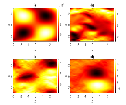
Figure 1: The evolution of solitary dipolar vortex [numerical solutions of (4) and (5)] is shown for $\psi\sim\omega_{g}H^{2}$ at different times: (a) $t=0$, (b) $t=20\omega_{g}^{-1}$, (c) $t=40\omega_{g}^{-1}$, and (d) $t=70\omega_{g}^{-1}$. Here, $x,~{}z\sim H$ with $\omega_{g}\sim 10^{-2}~{}\mathrm{s}^{-1}$ and $H\sim 10$ Km.

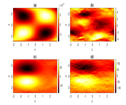
Figure 2: The evolution of dipolar vortex [numerical solutions of (5) and (10)] with an effect of $\eta=0.2\omega_{g}$ is shown for $\psi\sim\omega_{g}H^{2}$ at different times: (a) $t=0$, (b) $t=20\omega_{g}^{-1}$, (c) $t=50\omega_{g}^{-1}$, and (d) $t=70\omega_{g}^{-1}$. Here, $x,~{}z\sim H$ with $\omega_{g}\sim 10^{-2}~{}\mathrm{s}^{-1}$ and $H\sim 10$ Km.

II-B Evolution of chaos

We note in Sec. II-A that the particular system (4) and (5) or more generally, the system (5) and (10), which are multi-dimensional, can admit localized dipolar vortex solutions with finite wave energy or a solution whose amplitude decays due to dissipation. However, in the nonlinear interaction there may be a regime where a few coupled IGW modes are more active than the remaining ones. In this case, a low-dimensional temporal model can describe some other important basic features of the full dynamics. Such cases are quite typical in the plasma wave turbulence [23]. Thus, considering a class of solutions of (5) and (10) in the form [7, 8]

$$\psi =\left[a(t)\sin(k_{0}x)+b(t)\cos(k_{0}x)+\omega_{0}\right]z/k_{0},$$ (19)

$$\chi =\left[\alpha(t)\sin(k_{0}x)+\beta(t)\cos(k_{0}x)+\gamma(t)\right]z,$$ (20)

where $k_{0}$ and $\omega_{0}$ are constants, we obtain the following coupled dimensionless equations for IGWs.

$$\dot{a} =-\tilde{\omega}_{0}b-s\beta-\eta^{\prime}a,$$

$$\dot{b} =\tilde{\omega}_{0}a+s\alpha-\eta^{\prime}b,$$

$$\dot{\alpha} =-\omega_{0}^{\prime}\beta+b\gamma-b,$$

$$\dot{\beta} =\omega_{0}^{\prime}\alpha-a\gamma+a,$$

$$\dot{\gamma} =-a\beta+\alpha b.$$ (21)

Here, the overdot denotes differentiation with respect to $t$. Also, the variables $a$ and $b$ are normalized by $\omega_{g}$; $\alpha$, $\beta$ and $\gamma$ are normalized by $\omega_{g}^{2}$. Furthermore, $\eta^{\prime}=s\eta$ and $\tilde{\omega}_{0}=s\omega_{0}^{\prime}$, where $\omega_{0}^{\prime}=\omega_{0}/\omega_{g}$ and $s=\left(1+1/4Hk_{0}^{2}\right)^{-1}$. A careful numerical analysis of (21) reveals that the system can undergo through periodic, quasiperiodic and chaotic states for different sets of parameter values [8]. Figure 3 shows the bifurcation diagram [subplot (a)] and the maximum Lyapunov exponent [subplot (b)] with respect to the parameter $\eta^{\prime}$ associated with the Pedersen conductivity. It is found that in absence of the Ampére force (for which $\eta^{\prime}=0$), the system (4) and (5) exhibits chaos as evident from the positive Lyapunov exponent [subplot (b)]. However, the Lyapunov exponent tends to assume zero or negative values with increasing values of $\eta^{\prime}$. As a result, since the dissipation due to the Pedersen conductivity enters the picture, several asymptotic dynamics is seen to occur where the flow volume shrinks exponentially. Figure 4 shows that a chaotic strange attractor forms at $\eta^{\prime}=0$. However, as its value increases, the trajectories tend to move towards a fixed point via chaotic transits. The detailed investigation of the chaotic dynamics of (5) and (10) is limited to the present work. Nevertheless, a detailed dynamical study on a particular system (4) and (5) can be found in [8]. Here, one should note that some normalization issues occurred in the numerical analysis of [8] can easily be fixed if one simply considers the values of $\omega_{0}$ as those of $\omega_{0}/\omega_{g}$ and disregard the values of $\omega_{g}\sim 1$, because due to the normalization of $a,~{}b$ by $\omega_{g}$ and $\alpha,~{}\beta,~{}\gamma$ by $\omega_{g}^{2}$, the coefficient $\omega_{g}^{2}$ appeared in (6) of [8] should disappear.

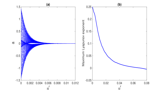
Figure 3: The bifurcation diagram [subplot (a)] and the maximum Lyapunov exponent [subplot (b)] are shown with respect to the dissipative parameter $\eta^{\prime}=\eta/\left(1+1/4Hk_{0}^{2}\right)$ for the evolution of IGWs. The other parameter values are $\omega_{0}^{\prime}=0.3$ and $s=0.4$. Here, $\eta^{\prime}=0$ correspond to the system (4) and (5), whereas $\eta^{\prime}\neq 0$ corresponds to the dissipative system (5) and (10). It is seen that the Pedersen conductivity $\eta$ has the effect of forbidding the occurrence of chaos in the nonlinear interaction of IGWs.

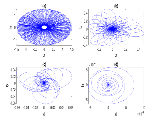
Figure 4: Trajectories flow of IGWs in phase space is shown for different values of $\eta^{\prime}$: (a) $\eta^{\prime}=0$, (b) $\eta^{\prime}=0.01$, (c) $\eta^{\prime}=0.02$, and $\eta^{\prime}=0.03$. The other parameter values are $\omega_{0}^{\prime}=0.3$ and $s=0.4$. Here, $\eta^{\prime}=0$ correspond to the system (4) and (5), whereas $\eta^{\prime}\neq 0$ corresponds to the dissipative system (5) and (10). Several asymptotic dynamics is seen where for a dissipative dynamical system volume shrinks exponentially: (a) chaotic strange attractor; (b) and (c) asymptotic fixed point dynamics via chaotic transit; (d) fixed point.

III Conclusion

We have studied the dynamical evolution of low frequency internal gravity waves (IGWs) in the weakly ionized Earth’s ionosphere. Starting from a set of fluid equations relevant for incompressible conducting fluids, we have derived a set of coupled equations which are shown to admit localized dipolar solitary vortices. Both the analytical and numerical approach are performed to show that in absence of the Pedersen conductivity stationary dipolar vortex structures can be formed with finite wave energy which can propagate with supersonic velocity for a longer time and that IGWs can evolve into chaotic states due to wave-wave interactions in a low dimensional dimensional model. The latter, however, predicts some basic features of the full system and is useful in the context of wave turbulence in conducting fluids [23]. As the dissipation due to the Pedersen conductivity enters the picture, the dipolar vortex structure tends to disappear due to the energy loss and the chaotic system evolves towards a stable fixed point. The results should be useful for understanding the remarkable features of low frequency internal gravity waves as well as the evolution of dipolar solitary vortices and chaotic flows associated with them in stratified weakly ionized plasmas that are relevant in the Earth’s ionosphere. The vortex structures so formed carry trapped particles and can play crucial roles in transportation of atmospheric components along the vertical direction thereby increasing the neutral density in the atmosphere at this height. Such density hike may increase the recombination rate of oxygen atoms and hence increase the intensity of night-sky radiation (with longer wavelengths $\sim 550$ nm) that are observed before strong earthquakes. This enhancement of the radiation spectra can be useful for predicting earthquakes [6].

References

- [1] J. R. Holton and G. J. Hakim, An Introduction to Dynamic Meteorology. USA: Academic Press, 2012.
- [2] D. Fritts and M. Alexander, “Gravity wave dynamics and effects in the middle atmosphere,” Reviews of Geophysics, vol. 41, p. 1003, 2003.
- [3] G. Swenson and P. Espy, “Observations of 2-dimensional airglow structure and na density from the aloha, october 9, 1993 ‘storm flight’,” Geophysical Research Letters, vol. 22, pp. 2845–2848, 1995.
- [4] R. H. Picard, R. O’Neil, H. Gardiner, J. Gibson, J. Winick, W. Gallery, A. T. Stair, P. Wintersteiner, E. R. Hegblom, and E. Richards, “Remote sensing of discrete stratospheric gravity-wave structure at 4.3-µm from the msx satellite,” Geophysical Research Letters, vol. 25, pp. 2809–2812, 1998.
- [5] N. Mitchell and V. Howells, “Vertical velocities associated with gravity waves measured in the mesosphere and lower thermosphere with the eiscat vhf radar,” Annales Geophysicae, vol. 16, pp. 1367–1379, 1998.
- [6] W. Horton, T. Kaladze, J. V. Dam, and T. Garner, “Zonal flow generation by internal gravity waves in the atmosphere,” Journal of Geophysical Research, vol. 113, 2008.
- [7] L. Stenflo, “Acoustic solitary vortices,” Physics of Fluids, vol. 30, pp. 3297–3299, 1987.
- [8] A. Roy, S. Roy, and A. P. Misra, “Dynamical properties of acoustic-gravity waves in the atmosphere,” Journal of Atmospheric and Solar-Terrestrial Physics, vol. 186, pp. 78–81, 2019.
- [9] N. C. Pati, P. C. Rech, and G. C. Layek, “Multistability for nonlinear acoustic-gravity waves in a rotating atmosphere,” Chaos: An Interdisciplinary Journal of Nonlinear Science, vol. 31, no. 2, p. 023108, 2021. [Online]. Available: https://doi.org/10.1063/5.0020319
- [10] D. Shaikh, P. K. Shukla, and L. Stenflo, “Spectral properties of acoustic gravity wave turbulence,” Journal of Geophysical Research: Atmospheres, vol. 113, no. D6, 2008. [Online]. Available: https://agupubs.onlinelibrary.wiley.com/doi/abs/10.1029/2007JD009305
- [11] D. Chatterjee and A. Misra, “Effects of coriolis force on the nonlinear interactions of acoustic-gravity waves in the atmosphere,” Journal of Atmospheric and Solar-Terrestrial Physics, vol. 222, p. 105722, 2021.
- [12] T. Kaladze, O. Pokhotelov, H. Shah, M. Khan, and L. Stenflo, “Acoustic-gravity waves in the earth’s ionosphere,” Journal of Atmospheric and Solar-Terrestrial Physics, vol. 70, no. 13, pp. 1607–1616, 2008. [Online]. Available: https://www.sciencedirect.com/science/article/pii/S1364682608001727
- [13] T. Kaladze, W. Horton, T. Garner, J. V. Dam, and M. L. Mays, “A method for the intensification of atomic oxygen green line emission by internal gravity waves,” Journal of Geophysical Research, vol. 113, p. A12307, 2008.
- [14] V. Bulatov and Y. Vladimirov, “Generation of internal gravity waves far from moving non-local source,” Symmetry, vol. 12, no. 11, 2020. [Online]. Available: https://www.mdpi.com/2073-8994/12/11/1899
- [15] V. E. Zakharov, “Collapse of langmuir waves,” Soviet Physics JETP, vol. 35, p. 908, 1972. [Online]. Available: http://www.jetp.ac.ru/cgi-bin/e/index/e/35/5/p908?a=list
- [16] J. T. Mendonça, O. G. Onishchenko, O. A. Pokhotelov, and L. Stenflo, “Wave-kinetic description of atmospheric turbulence,” Physica Scripta, vol. 89, no. 12, p. 125004, dec 2014. [Online]. Available: https://doi.org/10.1088/0031-8949/89/12/125004
- [17] J. T. Mendonça and L. Stenflo, “Acoustic-gravity waves in the atmosphere: from zakharov equations to wave-kinetics,” Physica Scripta, vol. 90, no. 5, p. 055001, apr 2015. [Online]. Available: https://doi.org/10.1088/0031-8949/90/5/055001
- [18] T. Kaladze, L. V. Tsamalashvili, and D. T. Kaladze, “Electromagnetic internal gravity waves in an ideally conducting medium,” 2018 XXIIIrd International Seminar/Workshop on Direct and Inverse Problems of Electromagnetic and Acoustic Wave Theory (DIPED), pp. 35–38, 2018.
- [19] T. Kaladze, L. Tsamalashvili, and D. Kaladze, “Electromagnetic internal gravity waves in an ideally conducting incompressible medium,” Journal of Atmospheric and Solar-Terrestrial Physics, vol. 182, pp. 177–180, 2019.
- [20] L. Stenflo and Y. A. Stepanyants, “Acoustic-gravity modons in the atmosphere,” Annales Geophysicae, vol. 13, p. 973–975, 1995.
- [21] T. Šindelářová, D. Burešová, and J. Chum, “Observations of acoustic-gravity waves in the ionosphere generated by severe tropospheric weather,” Studia Geophysica et Geodaetica, vol. 53, pp. 403–418, 2009.
- [22] P. K. Shukla and A. A. Shaikh, “Dust-acoustic gravity vortices in a nonuniform dusty atmosphere,” Physica Scripta, vol. T75, no. 1, p. 247, 1998. [Online]. Available: https://doi.org/10.1238/physica.topical.075a00247
- [23] S. Banerjee, A. P. Misra, P. K. Shukla, and L. Rondoni, “Spatiotemporal chaos and the dynamics of coupled langmuir and ion-acoustic waves in plasmas,” Phys. Rev. E, vol. 81, p. 046405, Apr 2010. [Online]. Available: https://link.aps.org/doi/10.1103/PhysRevE.81.046405