Immersed boundary approach to biofilm spread on surfaces

Abstract

We propose a computational framework to study the growth and spread of bacterial biofilms on interfaces, as well as the action of antibiotics on them. Bacterial membranes are represented by boundaries immersed in a fluid matrix and subject to interaction forces. Growth, division and death of bacterial cells follow dynamic energy budget rules, in response to variations in environmental concentrations of nutrients, toxicants and substances released by the cells. In this way, we create, destroy and enlarge boundaries, either spherical or rod-like. Appropriate forces represent details of the interaction between cells, and the interaction with the environment. Numerical simulations illustrate the evolution of top views and diametral slices of small biofilm seeds, as well as the action of antibiotics. We show that cocktails of antibiotics targeting active and dormant cells can entirely eradicate a biofilm.

I Introduction

Biofilms are formed by bacteria glued together by a self-produced polymeric matrix and attached to a moist surface biofilm . The polymeric envelop makes biofilms extremely resistant to antibiotics, disinfectants and chemical or mechanical aggressions Hoiby . Experiments reveal that their structure varies according to environmental conditions. When they grow in flows streamers ; Laspidou ; Picioreanu_fluids ; ibm_deformation , we see scattered bacteria immersed in large chunks of polymer. When they form on interfaces with air or tissue, volume fractions of polymer are very small Seminara ; Picioreanu_surface ; Allen and biofilms resemble aggregates of spherical or rod-like particles, see Figure 1 for a view of very early stages. As they mature, three dimensional sheets are formed, see Figure 2.

Modeling bacterial growth in the biofilm habitat is a complex task due to the need to couple cellular, mechanical and chemical processes acting on different times scales. Many approaches have been proposed, ranging from purely continuous models Seminara to agent based descriptions Laspidou ; Picioreanu_fluids ; ibm_deformation ; Picioreanu_surface ; Allen and hybrid models combining both poroelastic ; solid/fluid . Complexity increases when we aim to take bacterial geometry into account, issue that we intend to address here borrowing ideas from immersed boundary (IB) methods Peskin02 . These methods have already been adapted to simulate different aspects of biofilms in flows, such as finger deformation ibm_deformation , attachment of floating bacteria ibm_adhesion , and viscoelastic behavior ibm_rheology . Cell growth and division were addressed by removing the incompressibility constraint on the surrounding flow and including ‘ad hoc’ inner sources ibm_division . Recent extensions to multicellular growth consider closely packed deformable cells attached to each other ibm_tumor ; ibm_multicellular . Biofilms growing on interfaces differ from multicellular tissues in several respects. First, bacterial shapes are more rigid, usually spheres or rods. Second, bacteria remain at a short, but variable, distance of each other. To describe their evolution we need to take into account at least:

• Bacterial activities, such as growth, division and death in response to the environmental conditions.

• Chemical processes, such as diffusion of oxygen, nutrients, and toxicants (waste products, antibiotics) and production of autoinducers.

• Mechanical processes, such as the interaction of the fluid with the immersed structures and the interaction between the structures themselves.

These processes evolve in different time scales. Compared to cellular processes, which develop in a time scale of hours, mechanical and chemical processes are quasi-stationary. The inherent time scale for them would be seconds. Fast flow processes like adhesion or motion carried by a flow are not relevant for biofilms spreading on a surface. Instead, water absorption from the substrate in the time scale of growth is a factor to consider. Variations in the biofilm are driven by cellular activities, in a time scale of hours, through changes in the immersed boundaries due to cell growth, division, and death Seminara ; Hera ; poroelastic . These processes are influenced by the secretion of autoinducers and the production of waste products and polymers Seminara ; Hera ; poroelastic .

Here, we propose a computational model that combines an IB description of cellular arrangements and mechanical interactions with a dynamic energy budget representation of bacterial activity and chemical processes, including the action of toxicants. Modeling biofilm response to antibiotics is a crucial issue in their study Hoiby . The paper is organized as follows. Section II introduces the submodels for the different mechanisms. Section III nondimensionalizes the equations. Computational issues are discussed in Section IV, while presenting numerical simulations for horizontal spread. Section V considers spread of slices on barriers. Finally, Section VI shows how biofilm extinction can be achieved combining two types of antibiotics, one targeting active cells in the outer layers and another one targeting dormant cells in the biofilm core. Section VII summarizes our conclusions.

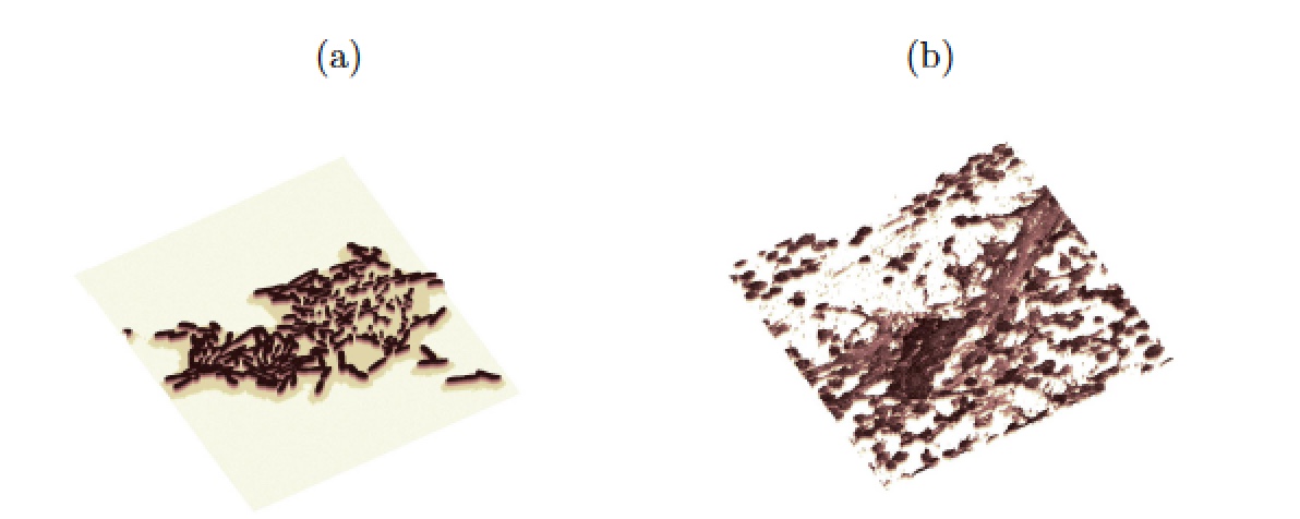
Figure 1: Schematic view of the early stages of a biofilm growing on a surface: Bacteria plus polymeric slime for (a) rod-like bacteria, (b) spherical bacteria.

Figure 2: Scheme of a vertical slice of a biofilm seed.

II Model

Taking the IB point of view Peskin95 ; Peskin02 , we consider the biofilm as a collection of spherical or rod-like cells, represented by their boundaries, immersed in a viscous fluid and subject to forces representing interactions, which are influenced by cell activity as we describe next. We will formulate the model in 2D.

II.1 Immersed boundary representation

Let us first describe the basic geometrical arrangement. To fix ideas, we consider the schematic structure depicted in Figure 1, a region $\Omega$ containing fluid and bacteria. We characterize bacteria by immersed boundaries representing their membranes. We assume the immersed boundaries have zero mass and are permeated by fluid. This liquid containing dissolved substances is considered incompressible. To simplify, we assume that the properties of the liquid are uniform.

The governing equations are established in Peskin95 ; Peskin02 . We summarize them here, including variations to adapt them to our biofilm framework:

• Incompressible Navier-Stokes equations in $\Omega$ with friction

  $${\partial\mathbf{u}\over\partial t}+\mathbf{u}\cdot\nabla\mathbf{u}=\nu\Delta\mathbf{u}-{1\over\rho}\nabla p+{1\over\rho}\mathbf{f}-{\alpha\over\rho}\mathbf{u},\quad{\rm div}(\mathbf{u})=0,$$ (1)

  where $\mathbf{u}(\mathbf{x},t)$ and $p(\mathbf{x},t)$ are the fluid velocity and pressure, while $\rho$, $\nu={\mu\over\rho}$ and $\alpha$ stand for the fluid density, kinematic viscosity and friction coefficient, respectively. The source $\mathbf{f}$ represents the force density, that is, force per unit volume.

• Force spread. The force $\mathbf{f}(\mathbf{x},t)$ created by the immersed boundary (IB) on the fluid is given by

  $$\mathbf{f}(\mathbf{x},t)=\int_{\Gamma}\mathbf{F}(\mathbf{q},t)\delta(\mathbf{x}-\mathbf{X}(\mathbf{q},t))\,d\mathbf{q},$$ (2)

  where $\mathbf{X}(\mathbf{q},t)$ is the parametrization of an immersed boundary $\Gamma,$ and $\mathbf{F}(\mathbf{q},t)$ the force density on it. The integration parameters $\mathbf{q}$ represent 3D angles.

• Velocity interpolation. The evolution equation for the IB

  $${\partial\mathbf{X}\over\partial t}=\int_{\Omega}\mathbf{u}(\mathbf{x},t)\delta(\mathbf{x}-\mathbf{X}(\mathbf{q},t))\,d\mathbf{x}+\lambda\big{(}(\mathbf{F}_{g}\cdot\mathbf{n})\mathbf{n}+\mathbf{F}_{ext}\big{)},$$ (3)

  is obtained correcting the no-slip condition with a term representing the contribution of the growth forces $\mathbf{F}_{g}$ on the IB. $\mathbf{n}$ stands for the unit outer vector. Notice that elastic forces within the IB do not contribute to this term because they are tangent to the normal $\mathbf{F}_{e}\cdot\mathbf{n}=0$. $\mathbf{F}_{ext}$ represents additional external forces that move bacteria as blocks, it includes at least interaction forces $\mathbf{F}_{i}.$ The adjusting factor $\lambda$ has units ${s\over kg}$.

Fluid-structure interaction is mediated by delta functions $\delta$. In practice, the $\delta$ function is replaced for computational purposes with approximations which scale with the meshwidth like $1/L^{3}$ in $3D$. Adequate regularizations are discussed in Peskin95 ; Peskin02 . We locate the immersed boundaries far from the borders of the computational domain, and enforce periodic boundary conditions for the fluid on them.

The above equations differ from standard IB models in two respects. First, we include friction in Navier-Stokes equations (1) as a way to represent the presence of polymeric threads hindering bacterial displacement. We could include threads joining the cells as part of the immersed structures, but we have chosen to represent their influence through friction in the fluid and interaction forces between the bacteria, to be described later. Second, we consider that the forces on the immersed boundaries are more general than just the elastic forces within it. This results in the addition of the term $(\mathbf{F}_{g}\cdot\mathbf{n})\mathbf{n}$ in equation (3) for their dynamics and allows to connect the growth forces to a description of cell metabolism.

II.2 Forces

In our case, the IB $\mathbf{X}$ is composed of many disjoint boundaries $\mathbf{X}_{j}$, $j=1,\ldots,N,$ representing the membranes of individual bacteria. The total force density $\mathbf{F}$ on the IB is the sum of several contributions.

• Elastic forces $\mathbf{F}_{e}$. In general, the elastic forces take the form $\mathbf{F}_{e}=-{\partial E\over\partial\mathbf{X}}$, where $E(\mathbf{X})$ is an elastic energy functional defined on the immersed boundary configuration $\mathbf{X}.$

  In a two dimensional setting, and assuming the boundary is formed by Hookean springs with zero rest length and parametrized by the angle $\theta$, the force would be

  $$\mathbf{F}_{e}=\frac{\partial}{\partial\theta}\left(K\frac{\partial\mathbf{X}}{\partial\theta}\right),$$ (4)

  for an elastic parameter $K$ (spring constants have units $N/m$). If we modify formula (2) to calculate a force per unit area $\mathbf{f}$

  $$\mathbf{f}(\mathbf{x},t)=\int_{0}^{2\pi}\mathbf{F}(\theta,t)\delta(\mathbf{x}-\mathbf{X}(\theta,t))\,d\theta,$$ (5)

  then $\delta$ should include units $1/L^{2}.$ These forces are calculated on each component $\mathbf{X}_{j}$, $j=1,\ldots,N$.

• Interaction forces $\mathbf{F}_{i}$. Bacteria adopt typically spherical (coccus), rod-like (Bacillus, Pseudomonas) or spiral (Vibrio) shapes. We focus on the first two types here. Bacteria in a biofilm loose their cilia and flagella, that is, their ability to move on their own. On one hand, there are repulsive forces between membranes that prevent bacteria from colliding. On the other, polymeric threads keep bacteria together. As mentioned earlier, we might add a thread network. However, we choose to represent their action by means of a friction term in Navier-Stokes equations. In this way, we avoid adding thread networks to keep cells together. We just need to separate the cells as they grow or divide.

  When the distances between bacteria are below a critical distance, repulsion forces act fast. The repulsion force $\mathbf{F}_{i,j}$ acting on each bacterium with boundary $\mathbf{X}_{j}$, $j=1,...,N$, depends on the distance between all pairs. For spherical bacteria, we set the force as follows:

  $$\begin{array}[]{l}\mathbf{F}_{i}=\sum_{j=1}^{N}\mathbf{F}_{i,j}\delta_{j},\\ \mathbf{F}_{i,j}=\left\{\begin{matrix}\displaystyle\sum_{n=1,n\neq j}^{N}\frac{\sigma}{d_{min}}\mathbf{n}_{{\rm cm},n,j}&\mbox{if }d_{j,n}\leq d_{min},\\ \displaystyle\sum_{n=1,n\neq j}^{N}{\sigma\left(1+\tanh\left({s_{p}-d_{j,n}\over v_{p}}\right)\right)\over 2d_{j,n}}\mathbf{n}_{{\rm cm},n,j}&\mbox{if }d_{j,n}>d_{min},\end{matrix}\right.\end{array}$$ (8)

  where $\sigma$ is the repulsion parameter with appropriate units, $d_{j,n}$ is the smallest distance between the curves defining bacteria $j$ and $n$, $N$ is the number of bacteria, and $\mathbf{n}_{{\rm cm},n,j}={\mathbf{X}_{c,j}-\mathbf{X}_{c,n}\over\|\mathbf{X}_{c,j}-\mathbf{X}_{c,n}\|}$ is the unit vector that joins the centers of mass, oriented from $n$ to $j$. Here, $\delta_{j}$ takes the value $1$ at the nodes of the cell boundary $\mathbf{X}_{j}$ and vanishes on other cell boundaries. Additional parameters govern the minimum value $d_{min}$ that $d_{j,n}$ can take, the order of magnitude of this force $s_{p}$, and the decay as the distance decreases $v_{p}$. These forces are similar for spheres and rods, changing the parameter values, see Table 1.

• Growth forces $\mathbf{F}_{g}$. Growth of spherical bacteria is described through variations in their radius, whereas rod-like bacteria grow in length. Assuming the rate of growth of their radius (resp. lengths) are known, the effect on each cell boundary would be, for spheres,

  $$\frac{dR_{j}}{dt}{\mathbf{X}_{j}-\mathbf{X}_{c,j}\over\|\mathbf{X}_{j}-\mathbf{X}_{c,j}\|}=\frac{dR_{j}}{dt}\mathbf{n},\quad j=1,\ldots,N,$$ (9)

  where $R_{j}$ and $\mathbf{X}_{c,j}$ denote the radius and center of the bacterium $\mathbf{X}_{j}$. For rods, growth forces act on the edges, forcing a change of length

  $${1\over 2}\frac{dL_{j}}{dt}\mathbf{l},\quad j=1,\ldots,N,$$ (10)

  where $\mathbf{l}$ is an outer unit vector along the rod axis. Notice that for spheres $(\frac{dR_{j}}{dt}\mathbf{n}\cdot\mathbf{n})\mathbf{n}=\frac{dR_{j}}{dt}\mathbf{n}$ whereas for rods $(\frac{dL_{j}}{dt}\mathbf{l}\cdot\mathbf{n})\mathbf{n}\sim 0$ except on the rod edges. We take $\mathbf{F}_{g}$ proportional to these growth factors.

  Our description of cell metabolism in Section II.3 provides the required equations for the time dynamics of radii $R_{j}$ and lengths $L_{j}$.

Finally, the total force we have to spread to the fluid through (2) or (5) is the sum of all the forces $\mathbf{F}=\mathbf{F}_{e}-\mathbf{F}_{i}+\mathbf{F}_{g}$.

II.3 Cellular activity

We describe bacterial metabolism by means of a dynamic energy budget approach Deb18 ; DebBook ; Debparameter :

• Dynamic energy budget equations for cell metabolism. Bacteria transform nutrients and oxygen in energy, which they use for maintenance, growth and division. In a biofilm, some cells undergo phenotypical changes and start performing new tasks. For instance, some become producers of exopolysaccharides, that is, the extracellular polymeric substances forming the biofilm EPS matrix. This is more likely for cells with scarce resources Hoiby ; Hera to sustain normal reproduction and growth.

  Given an aggregate formed by $N$ bacteria, their energy $e_{j}$ and volume $V_{j}$, $j=1,...,N,$ evolve according to

  $$\frac{de_{j}}{dt} =\nu^{\prime}\left(\frac{S}{S+K_{S}}-e_{j}\right), \nu^{\prime}=\nu e^{-\gamma\varepsilon}\left(1+{C_{out}\over K_{v}}\right)^{-1},$$ (11)

  $$\frac{dV_{j}}{dt} =\left(r_{j}\frac{a_{j}}{a_{M}}-h_{j}\right)V_{j}, \quad r_{j}=\left(\frac{\nu^{\prime}e_{j}-mg}{e_{j}+g}\right)^{+},$$ (12)

  where $\nu$ is the energy conductance, $\nu^{\prime}$ the conductance modified by exposure to a toxicant, $m$ the maintenance rate, $g$ the investment ratio, $a_{M}$ the target acclimation energy, $K_{S}$ a half-saturation coefficient, $K_{V}$ the noncompetitive inhibition coefficient and $\gamma$ the environmental degradation effect coefficient. The factor $r_{j}$ denotes the bacterial production rate. The symbol ⁺ stands for ‘positive part’, which becomes zero for negative values. The variables $S$, $C_{out}$, $\varepsilon$ denote the limiting nutrient/oxygen concentration, the concentration of toxic products, and the environmental degradation, respectively. Note that, for spherical bacteria with radius $R_{j}$, we have $V_{j}={4\over 3}\pi R_{j}^{3}$. In 2D, $V_{j}=\pi R_{j}^{2}$, and (12) implies

  $$2\frac{dR_{j}}{dt}=\Big{(}r_{j}\frac{a_{j}}{a_{M}}-h_{j}\Big{)}R_{j}.\quad$$ (13)

  For rod-like bacteria of radius $R$ and length $L_{j}$, $V_{j}\sim\pi R^{2}L_{j}$. In 2D, $V_{j}\sim 2RL_{j}.$ For ellipsoidal approximations, $V_{j}=\pi bL_{j},$ where $b$ is the small and $L_{j}$ the great semi-axes, with

  $$\frac{dL_{j}}{dt}=\Big{(}r_{j}\frac{a_{j}}{a_{M}}-h_{j}\Big{)}L_{j}.$$ (14)

  These equations must be complemented with equations for cell response to the degradation of the environment and the accumulation of toxicants. The cell undergoes damage, represented by aging $q_{j}$ and hazard $h_{j}$ variables, as well as acclimation, represented by the variable $a_{j}$. For $j=1,\ldots,N$, these additional variables are governed by

  $$\frac{dq_{j}}{dt}=e_{j}(s_{G}\rho_{x}{V_{j}\over V_{T}}q_{j}+h_{a})(\nu^{\prime}-r_{j})+k_{tox}C_{in,j}-(r_{j}+r_{e,j})q_{j},$$ (15)

  $$\frac{dh_{j}}{dt}=q_{j}-(r_{j}+r_{e,j})h_{j},$$ (16)

  $$\frac{dp_{j}}{dt}=-h_{j}p_{j},$$ (17)

  $$\frac{dC_{in,j}}{dt}=k_{in}C_{out}-k_{out}C_{in,j}-(r_{j}+r_{e,j})C_{in,j},$$ (18)

  $$\frac{da_{j}}{dt}=(r_{j}+r_{e,j})\left(1-\frac{a_{j}}{a_{M}}\right)^{+},$$ (19)

  where $\rho_{x}$ is the cell density, $s_{G}$ a multiplicative stress coefficient, $h_{a}$ the Weibull aging acceleration, and $k_{tox}$, $k_{in}$, $k_{out}$ the toxicity, influx coefficient and efflux coefficient of toxicants, respectively. The variable $C_{in,j}$ denotes the toxicant cellular density inside the cell and $p_{j}$ its probability of survival at time $t$. The factor $r_{e,j}$ is non zero only when the cell is an EPS producer (the values of the parameters $m$ and $g$ may be slightly different for such cells). In that case the rate of EPS production $r_{e,j}=kr_{j}+k^{\prime}$, where $k$ is the growth associated yield whereas $k^{\prime}$ is the non growth associated yield. The produced EPS is then

  $${dV_{e,j}\over dt}=r_{e,j}V_{j}.$$ (20)

  A fraction $\eta$ of the produced EPS stays around the cell, while a fraction $\eta\in(0,1)$ diffuses taking the form of a concentration of monomers $C_{e}$.

• Equations for concentrations. System (11)-(19) describes the metabolic state of each bacterium, and is coupled to reaction-diffusion equations for the relevant concentrations in $\Omega$:

  $$\frac{dS}{dt}=-\nu^{\prime}\frac{S}{S+K_{S}}\rho_{x}\displaystyle\sum_{j}{V_{j}\over V_{T}}\delta_{j}+d_{s}\Delta S-\mathbf{u}\cdot\nabla S,$$ (21)

  $$\frac{dC_{e}}{dt}=\eta\rho_{x}\displaystyle\sum_{j}r_{e,j}{V_{j}\over V_{T}}\delta_{j}+d_{e}\Delta C_{e}-\mathbf{u}\cdot\nabla C_{e},$$ (22)

  $$\frac{dC_{out}}{dt}=-C_{out}\displaystyle\sum_{j}r_{j}\delta_{j}+d_{c}\Delta C_{out}-\mathbf{u}\cdot\nabla C_{out},$$ (23)

  $$\frac{d\varepsilon}{dt}=\nu_{\varepsilon}\rho_{x}\displaystyle\sum_{j}(r_{j}+\nu_{m}m){V_{j}\over V_{T}}\delta_{j}+d_{\varepsilon}\Delta\varepsilon-\mathbf{u}\cdot\nabla\varepsilon,$$ (24)

  where $\nu_{\varepsilon}$ is the environmental degradation coefficient, $\nu_{m}$ is the maintenance respiratory coefficient and $d_{\varepsilon}$, $d_{s}$, $d_{e}$, $d_{c}$ the diffusion coefficients for degradation $\varepsilon$, limiting oxygen/nutrient concentration $S$, monomeric EPS $C_{e}$, and toxicants $C_{out}$, respectively. Here $\delta_{j}$ equals one in the region occupied by cell $j$, vanishes otherwise. $V_{T}$ is a reference volume. These equations are typically solved in the computational domain with no flux boundary conditions, except for $S$, which has a constant supply at the borders, and $C_{out}$ which is supplied at the borders as prescribed.

• Spread of cellular fields and interpolation of concentration fields. The system of ordinary differential equations (11)-(20) and reaction-diffusion equations (21)-(24) are coupled using a similar philosophy as that in IB models. However, now we transfer information not between curves and a two dimensional region but between confined regions occupied by bacteria and the whole computational domain:

  • Spread of fields defined on bacteria: Equations (21)-(24) use the cell volumes and rates as sources and sinks for the concentrations.

  • Interpolation of global fields on the bacteria: For each bacterium, system (11)-(20) uses the averaged values of $S$, $C_{out}$, $\varepsilon$ in the region occupied by the cell. $C_{out}$ represents the dissolved (extracellular) concentration of toxicants.

III Nondimensionalization of the equations

For computational purposes, it is essential to nondimensionalize properly these sets of equations. This allows us to identify relevant time scales for the different sets of equations, as well as controlling parameters. To remove dimensions we have to choose characteristic values for the different magnitudes. The characteristic length $L$ will tell us what part of the problem we want to focus on, that is, if we prefer to study what happens with the whole set of bacteria and do not want to spend a lot of computational time solving for details, or if we want to give more importance to what happens in the smaller areas. In our case we are interested in small cell aggregates, so we will have a characteristic length of $L=10[\rm\mu m]$ (microns, $1\mu$m $=10^{-6}$m), because it is about the maximum length of rod-like bacteria. In general, it will be the size of a small group of them. Time scales vary: microseconds for fluid processes, seconds for diffusion processes, and hours for cellular processes.

Let us first consider the IB submodel. We set a characteristic time $T=10^{-6}$[s]. In equation (1), the terms $(u_{t}+u\nabla u),\nu\Delta u$ have the same units, regardless of dimension. Let us set $p^{\prime}={p\over\rho}$, $\alpha^{\prime}={\alpha\over\rho}$. Then, $\mathbf{f}^{\prime}={\mathbf{f}\over\rho}$ has units of acceleration. Formally, one can just suppress one dimension in the variables and derivatives and use in 2D:

$${\partial\mathbf{u}\over\partial t}+\mathbf{u}\cdot\nabla\mathbf{u}=\nu\Delta\mathbf{u}-\nabla p^{\prime}+\mathbf{f}^{\prime}-\alpha^{\prime}\mathbf{u}.$$ (25)

As a reference acceleration, we set $a_{0}={E\over\rho L}={E_{s}\over\rho_{s}L}$, where $E_{s}$ is a longitudinal tension in units [${{\rm N}\over{\rm m}}$] (Young modulus for springs) and $\rho_{s}$ surface density in units [${{\rm kg}\over{\rm m}^{2}}]$. We know 3D values for the parameters. The Young modulus $E$ for bacterial membranes Youngcell1 lies in the range $100-200$ [MPa]. We set $E=150$ MPa = $150\times 10^{6}$ [${{\rm N}\over{\rm m^{2}}}$]. The density of water/biomass $\rho$ Seminara is about $10^{3}$ $[{{\rm kg}\over{\rm m}^{3}}]$. In this way, we find a value for $a_{0}$. Regarding the forces (2), for the elastic contribution we use (4) and (5) in 2D, which relates force per unit area to force with $\delta$ in units of ${1\over L^{2}}.$

Name	Symbol	Values	Units
Biomass density	$\rho$	$10^{3}$	$[\rm kg/m^{3}]$
Biomass viscosity	$\mu$	$100$	$[\rm kg/(m\,s)]$
Bacterial membrane Young Modulus	$E$	$150\times 10^{6}$	$[\rm kg/(m\,s^{2})]$

Table 1: Values for dimensional parameters of the IB submodel expressed in their standard units.

​​ $t\!=\!T\tilde{t}_{1}$ ​​	​​ $x\!=\!L\tilde{x}$ ​​	​​ $u\!=\!U\tilde{u}$ ​​	​​ ${p\over\rho}\!=\!P\tilde{p}$ ​​	​​ $\mathbf{F}\!=\!F\tilde{\mathbf{F}}$ ​​	​​ ${\mathbf{f}\over\rho}\!=\!{\mathbf{f}_{s}\over\rho_{s}}\!=\!a_{0}\tilde{\mathbf{f}}$ ​​
​​ $\delta\!=\!{1\over L^{2}}\tilde{\delta}$ ​​	​​ $K\!=\!K_{0}E_{s}$ ​​	​​ $U\!=\!{L\over T}$ ​​	​​ $P\!=\!{L^{2}\over T^{2}}$ ​​	​​ $F\!=\!E_{s}L$ ​​	​​ $a_{0}\!=\!{E\over L\rho}\!=\!{E_{s}\over L\rho_{s}}$ ​​
​​ $\alpha\!=\!\alpha_{0}{\rho\over T}$ ​​	​​ $\lambda\!=\!{\lambda_{0}\over E_{s}T}$ ​​	​​ $d_{j,n}\!=\!L\tilde{d}_{j,n}$ ​​	​​ $\sigma\!=\!\sigma_{0}E_{s}L^{2}$ ​​	​​ $s_{p}\!=\!s_{p,0}L$ ​​	​​ $v_{p}\!=\!v_{p,0}L$ ​​

Table 2: Change of variables used to nondimensionalize the IB equations. The $\tilde{}$ symbols are dropped for ease of notation after it. Dimensionless parameters $K_{0}$, $\alpha_{0}$, $\sigma_{0}$, $\lambda_{0}$, $s_{p,0}$, $v_{p,0}$, as well as the dimensionless numbers $Re$, $F_{c}$ and dimensional values for $\rho$, $\mu$, $E$ are given in Tables 1 and 3. The unknown value $E_{s}$ scales out. We assume $E/\rho=E_{s}/\rho_{s}$.

$Re={\rho L^{2}\over\mu T}$	$F_{c}={T^{2}E\over L^{2}\rho}$	$\alpha_{0}$	$\lambda_{0}$	$K_{0}$	$\sigma_{0}$	$d_{min,0}$	$s_{p,0}$	$v_{p,0}$
$10^{-3}$	$1.5\times 10^{3}$	$10^{-3}$	$10^{4}$	$0.15$	$0.05$	0.01	$0.01$	$0.01$

Table 3: Dimensionless control parameters for the IB submodel (26)-(31) when $L=10^{-5}$ [m] and $T=10^{-6}$ [s].

Performing the changes of variables indicated in Table 2 and dropping the $\tilde{}$ symbol for ease of notation we find the dimensionless IB system with parameters given by Tables 1-3:

$${\partial\mathbf{u}\over\partial t_{1}}\!+\!\mathbf{u}\!\cdot\!\nabla\mathbf{u}\!=\!{1\over Re}\Delta\mathbf{u}\!-\!\nabla p\!+\!F_{c}\mathbf{f}\!-\!\alpha_{0}\mathbf{u},\;{\rm div}(\mathbf{u})\!=\!0,$$ (26)

$$\mathbf{f}(\mathbf{x},t_{1})=\int_{0}^{2\pi}\mathbf{F}(\theta,t_{1})\delta(\mathbf{x}-\mathbf{X}(\theta,t_{1}))\,d\theta,\;\mathbf{X}=\cup_{j=1}^{N}\mathbf{X}_{j},$$ (27)

$${\partial\mathbf{X}\over\partial t_{1}}=\int_{\Omega}\mathbf{u}(\mathbf{x},t_{1})\delta(\mathbf{x}-\mathbf{X}(\mathbf{q},t_{1}))\,d\mathbf{x}+\lambda_{0}\big{(}(\mathbf{F}_{g}\cdot\mathbf{n})\mathbf{n}+\mathbf{F}_{ext}\big{)},$$ (28)

$$\mathbf{F}=\mathbf{F}_{e}+\mathbf{F}_{g}-\mathbf{F}_{i},$$ (29)

$$\mathbf{F}_{e}=\frac{\partial}{\partial\theta}\left(K_{0}\frac{\partial\mathbf{X}}{\partial\theta}\right),\;\mathbf{F}_{ext}=\mathbf{F}_{i},$$ (30)

$$\mathbf{F}_{i}=\left\{\begin{matrix}\displaystyle\sum_{j=1}^{N}\displaystyle\sum_{n=1,n\neq j}^{N}\frac{\sigma_{0}\delta_{j}}{d_{min,0}}\mathbf{n}_{{\rm cm},n,j}&\mbox{if }d_{j,n}\leq d_{min,0},\\ \displaystyle\sum_{j=1}^{N}\displaystyle\sum_{n=1,n\neq j}^{N}{\sigma_{0}\left(1+\tanh\left({s_{p,0}-d_{j,n}\over v_{p,0}}\right)\right)\delta_{j}\over 2d_{j,n}}\mathbf{n}_{{\rm cm},n,j}&\mbox{if }d_{j,n}>d_{min,0}.\end{matrix}\right.$$ (31)

The growth term $\mathbf{F}_{g}$ would be noticeable in the time scale of hours. In this scale, it is negligeable. The effect of growth would come through the boundaries, which move in the time scale of hours due to cellular processes. Here $\lambda_{0}\mathbf{F}_{g}\sim{T\over 3600}\sim 10^{-10}$. We can remove $\mathbf{F}_{g}$ from these equations. The effect of cell metabolism on bacterial boundaries will be calculated directly from the DEB equations.

Next, we consider the DEB equations for each cell. Recall that the variables $e,a,V_{j},p_{j},C_{in}$ are dimensionless. Hazard $h$ and aging $q$ have units $\rm hour^{-1}$ and $\rm hour^{-2}$, respectively. We remove the dimensions in the variables as indicated in Table 4. Taking into account the parameter values listed in Table 5, the remaining dimensions for parameters and rates are consistent. We work in a timescale $\tau=1$ hour, which is the natural step. Dropping again the symbol $\,\tilde{}\,$ for ease of notation we find for each cell $j$

$$\frac{de_{j}}{dt_{2}} =\tau\nu^{\prime}\left(\frac{S}{S+1}-e_{j}\right), \nu^{\prime}=\nu e^{-\gamma\varepsilon}\left(1+{C_{out}K_{S}\over K_{v}}\right)^{-1},$$ (32)

$$\frac{dV_{j}}{dt_{2}} =\left(\tau r_{j}\frac{a_{j}}{a_{M}}-h_{j}\right)V_{j}, \quad r_{j}=\left(\frac{\nu^{\prime}e_{j}-mg}{e_{j}+g}\right)^{+},$$ (33)

and

$$\frac{dq_{j}}{dt_{2}}=e_{j}(s_{G}\rho_{x}V_{j}q_{j}+h_{a}\tau^{2})\tau(\nu^{\prime}-r_{j})+\tau^{3}k_{tox}C_{in,j}-\tau(r_{j}+r_{e,j})q_{j},$$ (34)

$$\frac{dh_{j}}{dt_{2}}=q_{j}-\tau(r_{j}+r_{e,j})h_{j},$$ (35)

$$\frac{dp_{j}}{dt_{2}}=-h_{j}p_{j},$$ (36)

$$\frac{dC_{in,j}}{dt_{2}}=\tau k_{in}K_{s}C_{out}-\tau k_{out}C_{in,j}-\tau(r_{j}+r_{e,j})C_{in,j},$$ (37)

$$\frac{da_{j}}{dt_{2}}=\tau(r_{j}+r_{e,j})\left(1-\frac{a_{j}}{a_{M}}\right)^{+}.$$ (38)

For round bacteria in 2D, $V_{j}=\pi R_{j}^{2}$. Equation (33) provides the evolution of $\frac{dR_{j}}{dt_{2}}$. The evolution of the boundary due to cell metabolism is given by

$$\frac{\partial\mathbf{X_{j}}}{\partial t_{2}}=\frac{dR_{j}}{dt_{2}}{\mathbf{X}_{j}(\mathbf{q},t_{2})-\mathbf{X}_{c,j}(t_{2})\over\|\mathbf{X}_{j}(\mathbf{q},t_{2})-\mathbf{X}_{c,j}(t_{2})\|}.$$ (39)

In a similar way, if the cell is rod-like, its boundary evolves as given by (14).

$t=\tau t_{2}$

$h_{j}=\tilde{h}_{j}\tau^{-1}$

$q_{j}=\tilde{q}_{j}\tau^{-2}$

$V_{j}=\tilde{V}_{j}L^{2}$

$C_{out}=\tilde{C}_{out}K_{S}$

$V_{T}=L^{2}$

Table 4: Change of variables for nondimensionalization of the DEB model. We set $\tau=1$ [hour].

Symbol	Values	Units
$\nu$	$0.84768$	$[\rm hour^{-1}]$
$\gamma$	$1$	$[\rm n.d.]$
$K_{V}$	$154.82$	$[\rm mg/l]$
$K_{S}$	$0.1$	$[\rm mg/l]$
$C_{out}$	$0.20,0.78,1.56,3.13$	$[\rm mg/l]$
$g$	0.9766	$[\rm n.d]$
$m$	$0.1266$	$[\rm hour^{-1}]$
$\nu_{m}$	$0.054703$	$[\rm n.d.]$
$a_{M}$	$1.6703$	$[\rm n.d.]$
$s_{G}$	$0.8921\cdot 10^{-5}$	$[\rm l/mg]$
$h_{a}$	$1.4192\cdot 10^{-4}$	$[\rm hour^{-2}]$
$\nu_{\varepsilon}$	$0.23566/12000$	$[\rm l/mg]$
$k$	$2.2371$	$[\rm mg_{polymer}/mg_{cell}]$
$k^{\prime}$	$0.29$	$[\rm mg_{polymer}/(mg_{cell}hour)]$
$\eta$	$1/2$	$[\rm n.d.]$
$k_{out}$	$0.17251$	$[\rm hour^{-1}]$
$k_{in}$	$5.16\times 10^{-4}$	$[\frac{\rm l}{\rm mg\,hour}]$
$k_{tox}$	$5.416\times 10^{3}$	$[\rm hour^{-3}]$
$\rho_{x}$	$47000$	$[\rm mg/l]$

Table 5: Parameters of the DEB submodel (32)-(38) expressed in their standard units, adapted from Debparameter and Deb18 . Note that $[mg/l]=[10^{-6}kg/10^{-3}m^{3}]$. When inserted in the equations, all must be written in the same units of choice. Special attention must be paid to time units, which will be either hours or seconds, which requires multiplying or dividing by $3600.$

Finally, let us consider next the diffusion problems. The variable $\varepsilon$ is dimensionless. The concentrations $S$, $C_{e}$, $C_{out}$ have units $mg/l$. We set $C=K_{S}\tilde{C}$ for all the concentrations, $t=T_{d}\tilde{t}_{d}$ and same spatial scaling as before, as indicated in Table 6. Removing $\,\tilde{}\,$ for ease of notation again, we find the dimensionless equations:

$$\frac{dS}{dt_{d}}=-T_{d}\nu^{\prime*}\frac{S}{S+1}{\rho_{x}\over K_{S}}\displaystyle\sum_{j}V_{j}\delta_{j}+d_{s,0}D_{c}\Delta S-{T_{d}\over T}\mathbf{u}\!\cdot\!\nabla S,$$ (40)

$$\frac{dC_{e}}{dt_{d}}=\eta{\rho_{x}\over K_{S}}\displaystyle\sum_{j}T_{d}r_{e,j}^{*}V_{j}\delta_{j}+d_{e,0}D_{c}\Delta C_{e}-{T_{d}\over T}\mathbf{u}\!\cdot\!\nabla C_{e},$$ (41)

$$\frac{dC_{out}}{dt_{d}}=-C_{out}\displaystyle\sum_{j}T_{d}r_{j}^{*}\delta_{j}+d_{c,0}D_{c}\Delta C_{out}-{T_{d}\over T}\mathbf{u}\!\cdot\!\nabla C_{out},$$ (42)

$$\frac{d\varepsilon}{dt_{d}}=\nu_{\varepsilon}\rho_{x}T_{d}\!\displaystyle\sum_{j}(r_{j}^{*}\!+\!\nu_{m}m^{*})V_{j}\delta_{j}+d_{\varepsilon,0}D_{c}\Delta\varepsilon-{T_{d}\over T}\mathbf{u}\!\cdot\!\nabla\varepsilon,$$ (43)

with parameters given in Tables 5 and 7. Notice that $\nu^{\prime}$, $m$, $r_{j}$ and $r_{e,j}$ have units $\rm hour^{-1}$. To be used in these equations, they have to be expressed in units of $s^{-1}$, that is, divided by $3600$. We denote those values by $\nu^{\prime*}$, $m^{*}$, $r_{j}^{*}$ and $r_{e,j}^{*}$. The new diffusion coefficients will be large, the same as ${1\over Re}$. Both systems for fluids and concentrations should relax fast to an equilibrium. We are interested in stationary solutions, to be more precise, quasi-stationary, in the sense that they change with time when the immersed boundaries grow/split/die or the sources vary. That happens in a much longer time scale of hours.

​​ $t\!=\!T_{d}\tilde{t}_{2}$ ​​	​​ $x\!=\!L\tilde{x}$ ​​	​​ $V_{j}\!=\!L^{2}\tilde{V}_{j}$ ​​	​​ $S\!=\!K_{S}\tilde{S}$ ​​	​​ $C_{e}\!=\!K_{S}\tilde{C}_{e}$ ​​	​​ $C_{\rm out}\!=\!K_{S}\tilde{C}_{\rm out}$ ​​
$V_{T}=L^{2}$ ​​	​​ $D_{c}\!=\!D{T_{d}\over L^{2}}$ ​​	​​ $\nu^{\prime*}={\nu\over 3600}$ ​​	​​ $m^{*}={m\over 3600}$ ​​	​​ $r_{j}^{*}={r_{j}\over 3600}$ ​​	​​ $r_{e,j}^{*}={r_{e,j}\over 3600}$ ​​

Table 6: Change of variables used to nondimensionalize the equations for concentrations. The $\tilde{}$ symbols are dropped for ease of notation after it.

​​ $d_{\varepsilon,0}\!=\!22$ ​​

​​ $d_{s,0}\!=\!10$ ​​

​​ $d_{c,0}\!=\!5$ ​​

​​ $d_{e,0}\!=\!5$ ​​

​​ $D_{c}=10$ ​​

Table 7: Dimensionless parameters used in the concentration submodel (40)-(43) when $T_{d}=1$ [s] and $D=10^{-9}$ [m²/s].

IV Computational model for unconstrained spread

As said earlier, we are interested in two kinds of two dimensional reductions of three dimensional geometries representing biofilms spread on a surface. The first one consists of top views of early biofilm stages, see Figure 1. In the second one, we consider a 2D diametral slice of a 3D biofilm, see Figure 2. Let us focus on the first one, which can be handled with the equations and nondimensionalizations summarized in the previous two sections. The second one requires additional details that we will explain later.

To fix ideas, we consider that the computational region has a reference size around $100\times 100$ [$\rm\mu m$], that is, $10L\times 10L$ when $L=10$ [$\rm\mu m$]. We place a few bacteria at the center of this region, and let nutrients and toxicants diffuse from the boundaries. While a biofilm spreads on an interface with air, bacteria barely move, except when pushed by the rest. They grow up to their division or shrink until their death. The bacterial cluster tends to spread in the direction of the nutrient/oxygen concentration gradient. As they divide, bacteria occupy the free space and remain at a small distance from their neighbors. The average diameter of spherical bacteria is about $0.5-2.0$ [$\rm\mu$m]. For rod-shaped or filamentous bacteria, the average length is about $1-10$ [$\rm\mu$m] and diameter is about $0.25-1.0$ [$\rm\mu m$]. In our simulations we have taken for spheres $R=0.025-0.1$ [$\rm\mu m$], and for rods diameter $0.05-0.1$ [$\rm\mu m$] and length $0.1-1$ [$\rm\mu m$], nondimensionalized divided by the reference length $L$. Figure 3 illustrates some simulations.

Once we have fixed an initial bacterial arrangement and set initial conditions for all the variables we distinguish three blocks of equations. The DEB equations for each cell (32)-(39) are solved in the time scale of hours. In that time scale, the IB equations (26)-(31) and the equations for chemical processes (40)-(43) are quasistationary, changes are induced by growth, division, or destruction or boundaries according to the DEB submodel and the criteria for division, death or interaction. We solve them using time relaxation, that is, we solve the time dependent problems until the solutions relax to a stationary state. More precisely, we proceed as follows. First, we integrate the DEB system for all cells. Then, we relax the Ib2d model with interaction force to a stationary state, and finally the concentrations relax to their stationary state in the diffusion time scale. The process is schematized in Flowcharts 4 and 5. We next give details about the discretization and the initialization procedures.

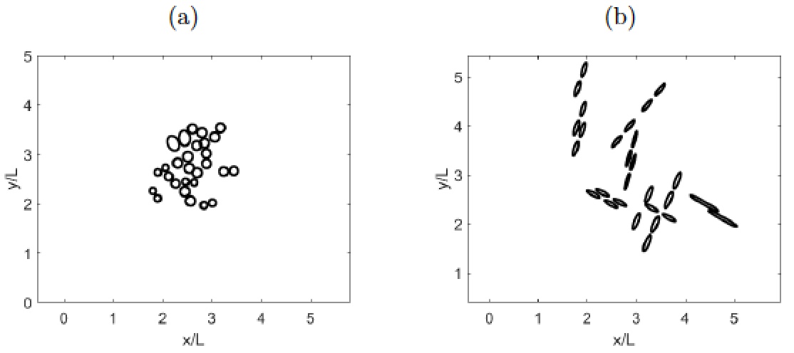
Figure 3: Snapshots of the evolution of a few bacteria with initial random sizes varying in the ranges specified in the text. Clusters formed by (a) round and (b) rod-like bacteria, see Video1 and Video2.

IV.1 Discretization

We define in the computational region a square mesh $\mathbf{x}_{i,j}=(x_{i},y_{j})$, $i,j=0,...,{\cal N}$, with step $dx=dy=h$ and nodes $x_{i}=x_{0}+idx$, $y_{j}=y_{0}+jdy$, where $x_{0}=y_{0}=0$, $x_{\cal N}=y_{\cal N}={\cal L}.$ We keep this mesh for all the submodels. However, the three submodels use different time discretizations. The main time mesh is $t\ell=\ell dt$, $\ell=0,...,{\cal M}$, up to the final time ${\cal T}={\cal M}dt.$ For each cell, the systems of ordinary differential equations (32)-(39) are discretized by a classical Runge-Kutta scheme on that mesh with step $dt=0.01.$ For the other two submodels we seek stationary solutions. We use the time dependence to implement time relaxation schemes to approximate them with adapted time steps. The reaction-diffusion equations (40)-(43) are discretized by classical explicit finite difference schemes. The whole set of equations for the immersed boundaries (26)-(30) are discretized using the finite difference schemes, quadrature rules and discrete $\delta_{h}$ functions described in Peskin02 .

The immersed boundaries are parametrized by the angle $\theta\in[0,2\pi]$. We use a mesh $\theta_{k}=kd\theta$, $k=0,...,{\cal K}$, on them. To prevent the distances between mesh points which form the immersed boundaries becoming too large as they grow, we increase the number of points in each of them at a certain rate, adding single points (in the case of round shapes) or opposite couples in the lateral walls (in the case of elongated shapes), at the sites where the distance between two neighboring mesh points is larger. This deserves further explanation, since it leads to work with a non uniform angle mesh and with angle dependent elastic moduli, which change as points are added. Given a mesh $\theta_{k}$ for a boundary $\mathbf{X}_{j}$, with steps $d\theta_{k}=\theta_{k}-\theta_{k-1}$, $k=1,...,{\cal K}$, we include a new point between sites $i-1$ and $i$ as follows:

• Set $d\theta_{i}=d\theta_{i}/2$, $d\theta_{i+1}=d\theta_{i}/2$, and $d\theta_{i+m}=d\theta_{i+m-1},$ $1<m<{\cal K}-i+1$.

• Set $\theta_{i}=\theta_{i-1}+d\theta_{i}$, $\theta_{i+1}=\theta_{i}+d\theta_{i+1}$, and $\theta_{i+m}=\theta_{i+m-1},$ $1<m<{\cal K}-i+1$.

• Set $\mathbf{X}_{j}(\theta_{i})={\mathbf{X}_{j}(\theta_{i-1})+\mathbf{X}_{j}(\theta_{i})\over 2}$, and $\mathbf{X}_{j}(\theta_{i+m})=\mathbf{X}_{j}(\theta_{i+m-1}),$ $0<m<{\cal K}-i+1$.

• Set $K_{j}(\theta_{i})=2K_{j}(\theta_{i})$, $K_{j}(\theta_{i+1})=2K_{j}(\theta_{i})$, and $K_{j}(\theta_{i+m})=K_{j}(\theta_{i+m-1}),$ $1<m<{\cal K}-i+1$, to prevent the reduction in the angle from changing the continuum limits.

• Set ${\cal K}={\cal K}+1.$

Additionally, we need rules for killing cells and dividing cells, which we detail next.

Figure 4: Flowchart for cell evolution in the time scale of hours.

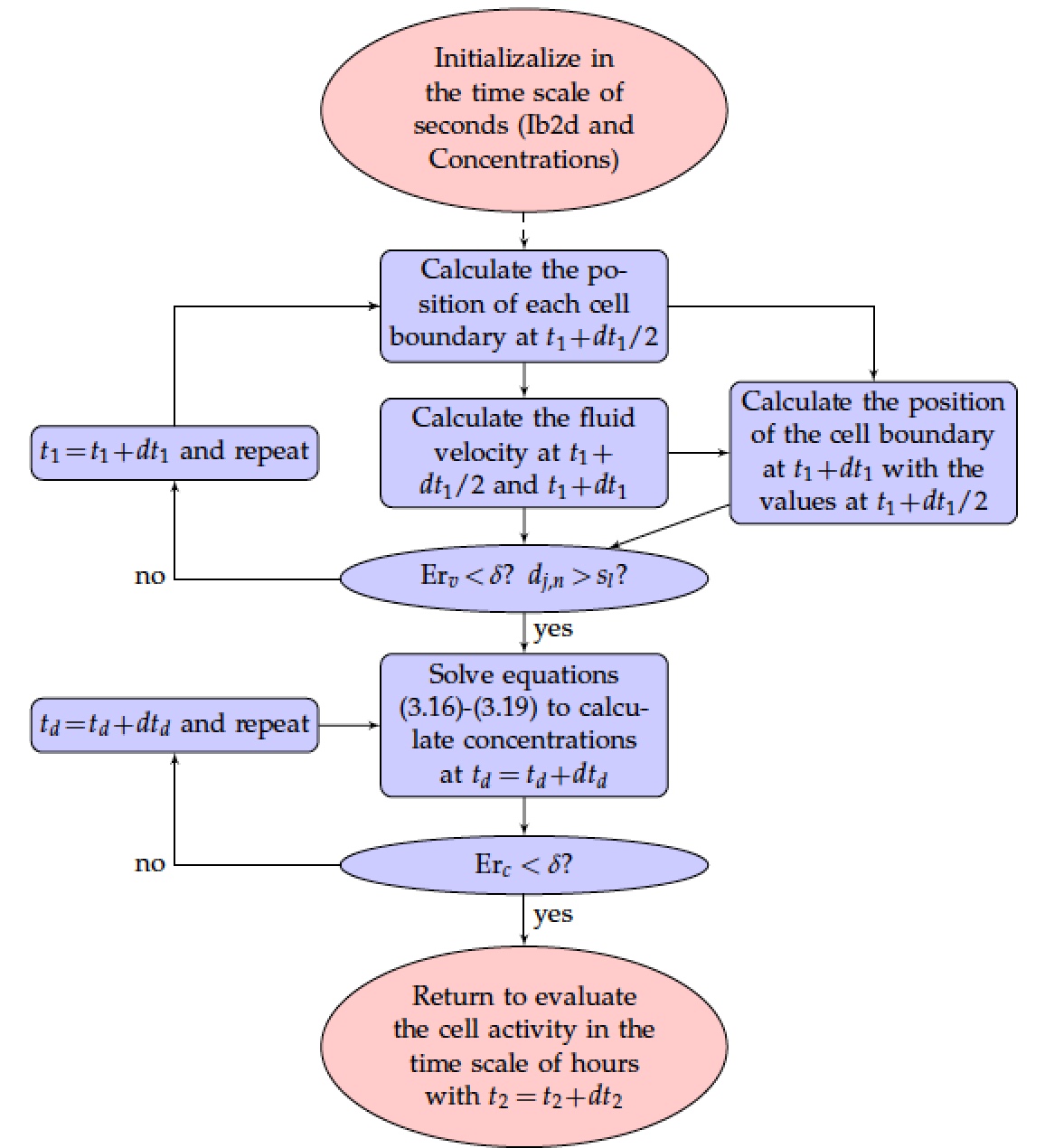
Figure 5: Flowchart for the submodels governing IB and chemical processes.

IV.2 Rules for division and death

Once the size of a bacterium $\mathbf{X}_{j}$ surpasses a critical perimeter, the cell divides with probability $P_{d,j}={S_{j}\over S_{j}+1},$ $S_{j}$ being the averaged value of the limiting concentration at the cell location, provided their aging acceleration $q_{j}$ is larger than a critical value $q_{c}$ (a way to indicate age, not to kill newborn cells). More precisely, for each cell boundary $\mathbf{X}_{j}$:

• We check whether $q_{j}>q_{c}=10^{-8}$.

• We check whether its length ${\rm Per}_{j}$ is larger than a critical perimeter ${\rm Per}_{c}=1.4\,{\rm Per}_{init,max}$ for sphera and ${\rm Per}_{c}=1.5\,{\rm Per}_{init,max}$ for rod-like bacteria, where ${\rm Per}_{init,max}$ is the maximum perimeter in the initialization step.

• We generate a random number $r\in(0,1)$ and check whether $P_{d,j}>r.$

Figures 6 and 7 illustrate the division process for spherical and rod-like bacteria. Division is completed in a few steps: the cell elongates and then splits conserving area. For spherical bacteria, if $V_{init}=\pi R_{init}^{2}$ is the volume before division, we have radius $R_{end}={R_{init}\over\sqrt{2}}$ for the two daughters. For rod-like bacteria, with initial volume $V_{init}=\pi ba_{init}$, being $b$ the smallest semi-axis, we have $a_{end}={a_{init}\over 2}$ for the two daughters, because $b$ is constant. We reset all the cell variables to their initial values after division, see Section IV.3.

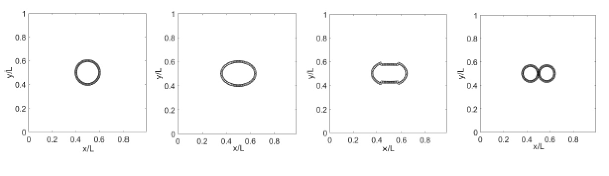
Figure 6: Snapshots of the division of a spherical bacterium.

Figure 7: Snapshots of the division of a rod-like bacterium.

Figure 8: Snapshots of the evolution of a circular biofilm formed by $100$ cells under the same conditions but different death treatment: (a) Shrinking dead cells (represented in red). We have $292$ alive cells and $108$ dead ones. (b) Erasing dead cells. We have $294$ alive cells and have erased $86$.

Similarly, the cell $\mathbf{X}_{j}$ dies with probability defined by $p_{j}$, $j=1,...N.$ We kill $\mathbf{X}_{j}$ when $1-p_{j}>{N_{init}\over N_{a}}+r\left(1-{N_{init}\over N_{a}}\right)$, where $N_{a}$ is the current number of bacteria, $N_{init}$ the initial number of bacteria and $r\in(0,1)$ a random number. When a bacterium dies we have two options: 1) erase the cell immediately, 2) keep it and solve only equations (33) for the volume, so that it shrinks slowly due to reabsorption, see Figure 8. The latter option may produces a more realistic evolution in some cases, to account for necrotic regions which otherwise would be erased. We solve the whole set of equations (32)-(39) for the living cells, but only Eq. (33) for the dead cell, fixing $h=h_{death}.$ For spheras, when the dead cell’s perimeter is below a minimum threshold ${\rm Per}_{m}=\pi dx$, $dx$ being the spatial discretization step, the cell disappears. For rod-like bacteria we take ${\rm Per}_{m}=2\pi b$, being $b$ the shortest semi-axis. The parameter $h_{death}$ governs the speed of the perimeter decrease. We choose to increase $h_{death}$ with the number of alive cells surrounding the dead one, since it represents reabsorption. More precisely, we set $h_{death,j}=h_{death,j}+dt{\rm Nc}_{C_{i}<Rd}$, where ${\rm Nc}_{C_{i}<Rd}$ is the number of cells whose center lies at a distance smaller than $Rd={3/L}$ for cell $j$ and $dt=dt_{2}.$

Figure 9: (a) Initial arrangement. Evolution at (b) $t=9$ h, (c) $t=12$ h, (d) $t=14$ h, (e) $t=20$ h. The simulation starts with $100$ cells and ends up with $286$ cells alive, $81$ dead (red) and $179$ already erased, see Video3.

IV.3 Initialization and boundary conditions

A typical geometry initialization is represented in Figure 9(a). We define $N$ non overlapping immersed boundaries (either spheres or rods) in the region $13L\times 13L$ for sphera and $17L\times 17L$ for rod-like bacteria, located inside a circle of a given radius. The centers, dimensions, axis orientation (when required), and number of points forming the boundaries, vary randomly about given values. Next,

• We create the cubic mesh of step $dx$ in that region to discretize the fluid and the reaction-diffusion equations.

• We set the initial velocity $\mathbf{u}$ equal to zero everywhere and periodic boundary conditions for the fluid velocity.

• A reference value $S_{0}=10$ is fixed as initial and Dirichlet boundary condition for the concentration at the borders of the computational region.

• We set $C_{e}(0)=0$ and $\varepsilon(0)=0$ everywhere and enforce zero Neumann boundary conditions for them.

• For the first simulations, we set $C_{out}(0)=0$ everywhere and enforce zero Dirichlet boundary conditions. Once the biofilm seed has evolved for some time, we switch to a Dirichlet boundary condition $C_{out}=3,\,7,\,30$ on the borders of the computational region. As initial condition for $C_{out}$ we use the profile obtained by relaxation of (42) with the boundary condition and without the convective term.

• For $j=1,...,N$ we set $V_{j}(0)$ equal to the initial dimensionless areas, $e_{j}(0)={S_{j}(x_{j},0)\over S_{j}(x_{j},0)+1}$, $x_{j}$ being the center of cell $j$, $V_{e,j}(0)=0$, $q_{j}(0)=0$, $h_{j}(0)=0.6$, $p_{j}(0)=1$, $a_{j}(0)=0$, and $C_{in,j}(0)=0$. When we divide a cell, they start with the same initial conditions, except $C_{in,j}$ in the presence of a toxicant, which divides a random percentage to one and the opposite to the other.

Figure 10: Evolution of the final configuration reached in Fig. 9 under the action of antibiotics. Snapshots for $C_{out}=3$ at (a) $t=1$ h, (b) $t=6$ h, and (c) $t=12$ h. The simulation ends with $260$ cells alive, $17$ dead (red) and $419$ already erased, see Video3a. Snapshots for $C_{out}=7$ at (d) $t=1$ h, (e) $t=5$ h, and (f) $t=12$ h. The simulation end with $213$ cells alive, $38$ dead (red) and $390$ already erased, see Video3b. Snapshots for $C_{out}=30$ at (g) $t=1$ h, (h) $t=3.5$ h, and (i) $t=10$ h. The simulation ends with $162$ cells alive, $6$ dead (red) and $354$ already erased, see Video3c. If we do not erase them, we have a necrotic outer layer of increasing thickness.

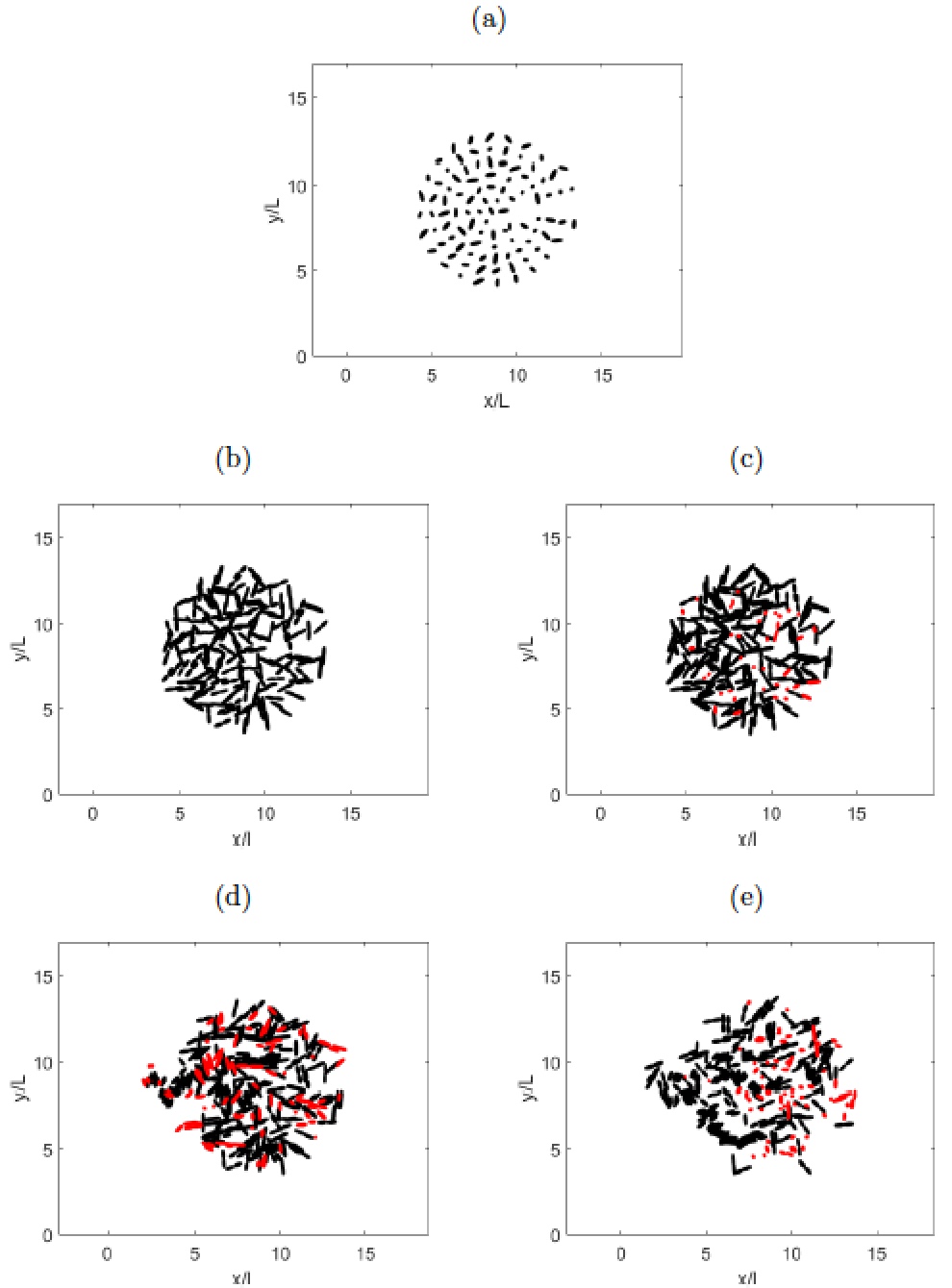
Figure 11: (a) Initialization. Evolution at (b) $t=9.5$ h, (c) $t=12$ h, (d) $t=14$ h and (e) $t=20$ h, without antibiotics. We started with $100$ bacteria, and ended with $289$ alive, $68$ dead (red) and $267$ disappeared, see Video4.

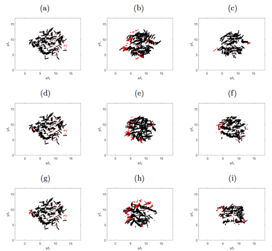
Figure 12: Evolution of the final configuration reached in Fig. 11 under the action of antibiotics. Snapshots for $C_{out}=3$ at (a) $t=1$ h, (b) $t=6.5$ h, and (c) $t=10$ h with $284$ alive, $14$ dead (red) and $358$ erased, see Video4a. Snapshots for $C_{out}=7$ at (d) $t=1$ h, (e) $t=7.5$ h, and (f) $t=10$ h with $278$ alive, $40$ dead (red) and $340$ erased, see Video4b. Snapshots for $C_{out}=30$ at (g) $t=1$ h, (h) $t=3$ h, and (i) $t=10$ h with $246$ alive, $34$ dead (red) and $346$ erased, see Video4c.

Figures 9-10 show a few snapshots of the evolution of a circular biofilm formed by spherical bacteria, without antibiotic and with antibiotics, respectively, see also Videos 3, 3a, 3b, 3c. The action of antibiotics would vary depending on parameters we have fixed, such as the toxicity, and the parameters governing the flux inside and outside the cells. We see that as the antibiotic presence is increased, growth slows down, less cells remain, and an outer necrotic region appears, that finally dissolves in the surrounding fluid and is absorbed by the remaining cells. The dynamics of dead cells depends on the governing parameters we choose to govern the reabsorption process. Figures 11-12 illustrate the evolution for rod-like bacteria, see also Videos 4, 4a, 4b, 4c.

As said earlier, we use a specific discretization of the Inmersed Boundary model, solving (26)-(31) by Fourier transforms Peskin95 ; Peskin02 . We use the time $t_{1}$ as an artificial time until the system relaxes to a stationary state, with step $dt_{1}=10^{-6}$. When the relative errors of the fluid-IB variables ${\rm Er}_{v}$ fall below a tolerance $\delta$, we use the time $t_{d}$ as an artificial time until the concentration system relaxes to a stationary state with a step $dt_{d}=10^{-9}$ for spheres and $dt_{d}=10^{-11}$ for rods, due to the convection factor $T_{d}/T=10^{6}$. When the relative errors ${\rm Er}_{c}$ fall below a tolerance $\delta$, we stop. We set $\delta=10^{-3}$. We also demand that the cells remain at a certain distance $s_{l},$ in these tests we have set $s_{l}=0.$

V Computational model in the presence of barriers

As mentioned earlier, we are interested in two kinds of two dimensional reductions. So far, we have considered the horizontal spread of a two dimensional cluster. We focus here on the arrangement depicted in Figure 2: a biofilm slice expanding on a surface. The model equations remain the same as in Sections III and IV. The main change concerns the geometry: we introduce a boundary orthogonal to the biofilm slice representing the interface on which it grows. We place bacteria on a semi-circle on top of it, see Figure 13(a). We will exploit the strategy developed in Section IV, including additional equations for the horizontal barrier. We impose on it the same equations as for the cell boundaries, without the growth force, and without interaction force (bacteria do not move the barrier). On the other hand, cells do notice the presence of the barrier and the corresponding interaction is included for them. Moreover, in equation (5), in front of the integral, we add a factor $0.001$ to account for higher density of the barrier and almost negligible barrier mobility due to fluid.

The main variations arise when working with rod-like bacteria. We set $dt_{d}=10^{-10}$. In this case, forces can generate a moment that rotate bacteria. This force creates a torque, $\mathbf{M}_{f}$, that then varies the angular momentum $\mathbf{L}$, and knowing the moment of inertia $\mathbf{L}=\mathbf{I}\mathbf{w}$, we obtain the angular velocity $\mathbf{w}$, $\mathbf{I}$ being the body’s inertia tensor.

$$\mathbf{M}_{f}=\mathbf{X}\times\mathbf{F}_{i},\quad{d\mathbf{w}\over dt}=\mathbf{I}^{-1}\mathbf{M}_{f}.$$ (44)

In two-dimensions, directions of $\mathbf{M}_{f}$ and $\mathbf{w}$ are perpendicular to the plane. Thus, we only need the moment of inertia of the axis perpendicular to the plane, which is $I={1\over 4}M(a^{2}+b^{2})$ for elliptical shapes, where $a$ is the long semi-axis, and $b$ the short one. $M$ is the mass of the bacteria, $M=\rho_{x}V$, where $\rho_{x}$ is bacterial density and $V$ its volume. In two-dimensions, they become surface density and area. In this way, we can add in Eq. (3) the following expression

$${\partial\mathbf{X}\over\partial t}=\mathbf{w}\times\mathbf{X}.$$ (45)

When we nondimensionalize, we need to include in the right hand side of Eq. (28) the term $\mathbf{w}\times\mathbf{x}$ with

$${d\mathbf{w}\over dt}=C_{f}\mathbf{I}_{0}^{-1}\mathbf{M}_{f},\quad\mathbf{M}_{f}=\mathbf{x}\times\mathbf{F}_{i},$$ (46)

where all terms are dimensionless, and $C_{f}=T^{2}{E_{s}L^{2}\over\rho_{x,s}L^{2}}={150\over 47}10^{-6}$ is a dimensionless number, calculated using ${E_{s}\over\rho_{x,s}}={E\over\rho_{x}}$. Moreover, $\mathbf{I}_{0}={1\over 4}M_{0}(a_{0}^{2}+b_{0}^{2})$, where $M_{0}=V$, $V=\pi a_{0}b_{0}$ is dimensionless bacterial area and $a_{0}=a/L$, $b_{0}=b/L$.

A new feature we wish to represent in this new set-up is the observation that fluid flows upwards through the horizontal barrier because the bacterial biofilm seed swells. We are representing the threads keeping together bacteria in the biofilm as interaction forces keeping bacteria at a distance. When the biofilm swells, those threads swell and elongate too. We model this fact changing the minimum distance between bacteria in the biofilm.

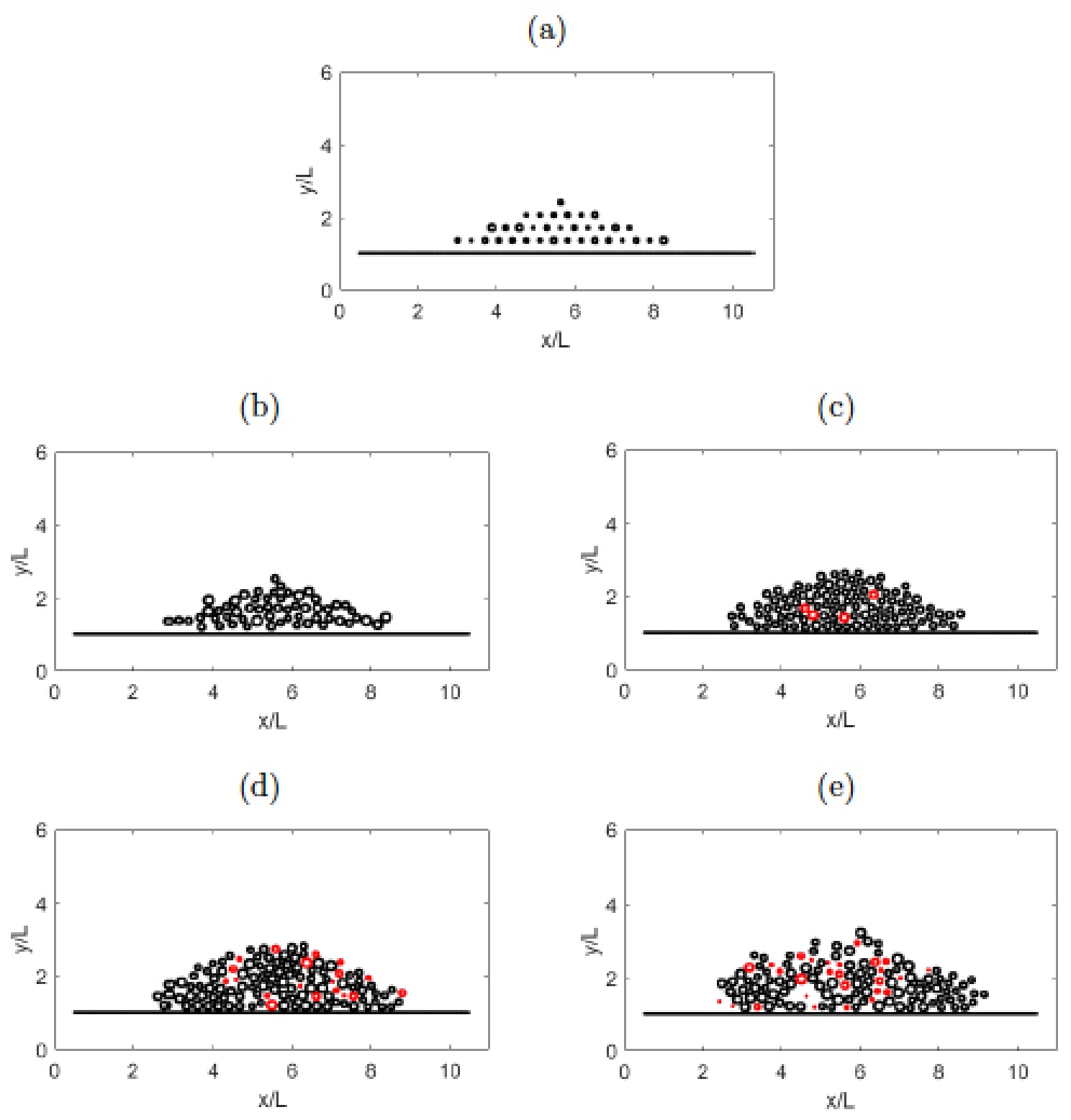
Figure 13: (a) Initial arrangement. Evolution at (b) $t=9$ h, (c) $t=12$ h, (d) $t=15$, (e) $t=20$ h. The simulation starts with with 34 cells and ends with $97$ alive cells, $27$ dead cells (red) and $58$ cells already erased, see Video5.

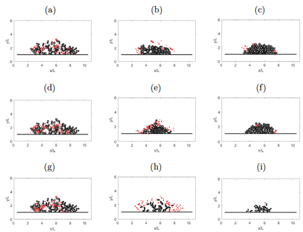
Figure 14: Evolution of the final configuration reached in Fig. 13 under the action of antibiotics. Snapshots for $C_{out}=3$ at (a) $t=1$ h, (a) $t=7.5$ h, and (c) $t=10$ h. The simulation ends with $77$ cells alive, $7$ dead (red) and $120$ erased, see Video5a. Snapshots for $C_{out}=7$ at (d) $t=1$ h, (e) $t=7$ h, and (f) $t=10$ h. The simulation ends with $69$ cells alive, $3$ dead (red) and $125$ erased, see Video5b. Snapshots for $C_{out}=30$ at (g) $t=1$ h, (h) $t=3.5$ h, and (i) $t=10$ h. The simulation ends with with $34$ cells alive, $2$ dead (red) and $116$ erased, see Video5c.

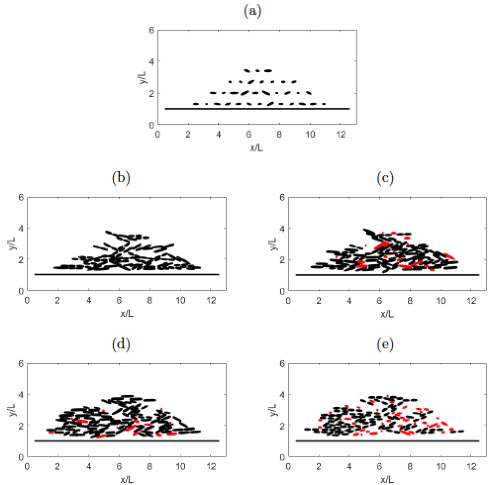
Figure 15: (a) Initial arrangement. Evolution at (b) $t=10$ h, (c) $t=14$ h, (d) $t=18$ h, (e) $t=20$ h. The simulation starts with $33$ cells and ends with $96$ cells alive, $41$ dead and $75$ erased, see Video6.

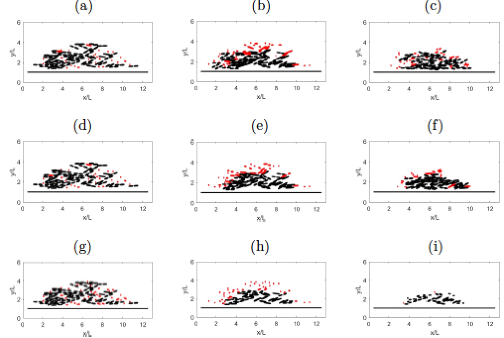
Figure 16: Evolution of the final configuration reached in Figure 15 under the action of antibiotics. Snapshots for $C_{out}=3$ at (a) $t=1$ h, (a) $t=4$ h, and (c) $t=10$ h. The simulation ends with $84$ cells alive, $29$ dead (red) and $108$ erased, see Video6a. Snapshots for $C_{out}=7$ at (d) $t=1$ h, (e) $t=4$ h, and (f) $t=10$ h with $58$ alive, The simulation ends with $17$ cells dead (red) and $115$ erased, see Video6b. Snapshots for $C_{out}=30$ at (g) $t=1$ h, (h) $t=3.5$ h, and (i) $t=10$ h. The simulation ends with $33$ cells alive, $2$ dead (red) and $105$ erased, see Video6c.

For spherical bacteria, we modify the repulsive force because it is not the same to push upwards than horizontally without the force of gravity. The force is of lesser magnitude and the repulsion occurs more gradually:

$$\mathbf{F}_{i}=\sum_{j=1}^{N}\mathbf{F}_{i,j}\delta_{j},\quad\mathbf{F}_{i,j}=\displaystyle\sum_{n=1,n\neq j}^{N-1}\sigma_{b}\,e^{-{d_{j,n}^{2}\over l_{sp}}}\mathbf{n}_{{\rm cm},n,j},$$ (47)

$\sigma_{b}$ is the repulsive parameter, and $l_{sp}$ sets the maximum distance, where the cells begin to repel. The latter term changes over time, as swelling causes the strings that separate the cells to grow. We have set

$$l_{sp}=l_{max}{1+\tanh\left(v_{s}\left(t-T_{p}\right)\right)\over 2}\quad s_{p2}=\sqrt{-\ln(v_{min})l_{sp}},$$ (48)

where $l_{max}=-{s_{max}^{2}\over\ln(v_{min})}$ and $v_{s}$ is related to the growth of this distance. It saturates at a certain time, we use an inflection point $T_{p}$, and a certain maximum length $l_{max}$. This value depends on the maximum separation of the cells $s_{max}$ and a minimum variation $v_{min}$. All of this affects the critical distance $s_{p2}$. All cells tend to be more or equal apart. Removing dimensions, the interaction force is as follows:

$$\mathbf{F}_{i}=\displaystyle\sum_{j=1}^{N}\displaystyle\sum_{n=1,n\neq j}^{N}\sigma_{b,0}\,e^{-{d_{j,n}^{2}\over l_{sp}}}\delta_{j}\mathbf{n}_{{\rm cm},n,j},$$ (49)

where $\sigma_{b}=\sigma_{b,0}LE_{s}=20E_{s}$, so $\sigma_{b,0}=20/L$. And $\tilde{l}_{sp}(t_{1})=l_{sp}(t_{1})/L^{2}$. We drop the symbol $\,\tilde{}\,$ for ease of notation. Parameters are collected in Table 8.

For rods there is anisotropy, the vertical direction being different from the horizontal one. We set

$$s_{p2}=t{s_{p,m}\over T_{m}},$$ (50)

where ${s_{p,m}\over T_{m}}$ is the slope to which the distance with respect to time ascends. We do not have to change the force because the interaction in one plane and the other are similar, the only difference being the growth of the distance. Removing dimensions

$$s_{p2}=t_{2}{s_{pm,0}\over T_{pm,0}}.$$ (51)

In either case, spheres or rods, we set $s_{l}=s_{p2}$ in the flowchart.

$s_{max,0}={s_{max}\over L}$	$l_{m,0}=-{s_{max}^{2}\over\ln(v_{min})L^{2}}$	$T_{p,0}={T_{p}\over\tau dt_{2}}$	$v_{min}$
$0.04$	$-{1.6\times 10^{-3}\over\ln(v_{min})}$	$6.5\over dt_{2}$	${dt_{2}\over 2dt_{1}\lambda_{0}\sigma_{b,0}}$
$s_{pm,0}={s_{pm}\over L}$	$T_{pm,0}={T_{pm}\over\tau dt_{2}}$	$v_{s,0}=\tau v_{s}$
$0.04$	$11\over dt_{2}$	$5\times 10^{-3}$

Table 8: Additional parameters for the simulations in the presence of an horizontal barrier.

In this second geometry, nutrients flow to bacteria through the horizontal immersed boundary on top of which they grow, whereas toxicants flow from the top. As for the initialization, besides the $N$ immersed boundaries representing bacteria, we include a lower barrier which does not touch the borders of the computational region. Boundary conditions for concentrations change. We fix Dirichlet boundary conditions for $S$ and $C_{e}$ on the lower computational border, and on the lateral ones up to the height of the horizontal immersed boundary. Zero Neumann boundaries are imposed on the rest. For $C_{out}$, the situation is reversed. Zero Neumann boundary conditions on the lower part, and Dirichlet on the upper one.

Figures 13 and 14 illustrate the evolution in the case of spherical bacteria, with and without antibiotics. Notice the formation of inner gaps or channels in the structure. When antibiotics are added, outer necrotic region finally erased appear too. Figures 15 and 16 illustrate the evolution in the case of rod-like bacteria.

VI Biofilm extinction

In this Section, we consider the possibility of driving a biofilm to extinction by an adequate combination of antibiotics Hoiby . The death criterion we employed in the previous sections allows the biofilm to grow but it prevents the total number of bacteria from dropping below the initial value. For decaying biofilms, the death criterion used in Deb18 is more adequate: we kill a cell $\mathbf{X}_{j}$ when $p_{j}<r{N_{a}\over N_{init}}$, being $N_{init}$ the number of bacteria just before administering the antibiotics. In Figure 17, we revisit simulations (a)-(c) and (d)-(f) from Figure 9 with this new criterion. Clinical tests Hoiby point out the convenience of combining antibiotics targeting different types of cells within the biofilm to be able to eradicate them. We consider here a cocktail of two antibiotics. One of them targets dormant cells with little energy, which are located in the inner biofilm core (the antibiotic colistin, for instance). We represent that effect using a toxicity coefficient $k_{tox,1,j}$ which decreases wth the cell energy. The other one targets cells with high energy, which divide actively, and tend to be located in the outer biofilm regions (penicillins, for instance). We represent that effect by a toxicity coefficient $k_{tox,2,j}$ which increases with the cell energy. More precisely, we have used the following expression

$$k_{tox,1,j}=k_{tox}e^{10(e_{m}-e_{j})},\quad k_{tox,2,j}=k_{tox}e^{10(e_{j}-e_{m})},\quad e_{m}=0.5.$$ (52)

We modify the model to include two equations similar to (42) for the antibiotic concentration with toxicity coefficients (52) and the corresponding two equations (37) for the antibiotic concentration inside the cells. Also, we set $C_{out}=C_{out,1}+C_{out,2}$ in the definition of (32) for $\nu^{\prime}$ and replace in eq. (34) the term $k_{tox}C_{in,j}$ by $k_{tox,1,j}C_{in,1,j}+k_{tox,2,j}C_{in,2,j}$. Revisiting the simulations in Figure 9 with these new choices, we are able to drive the biofilm to extinction, see Figure (17) (g)-(i).

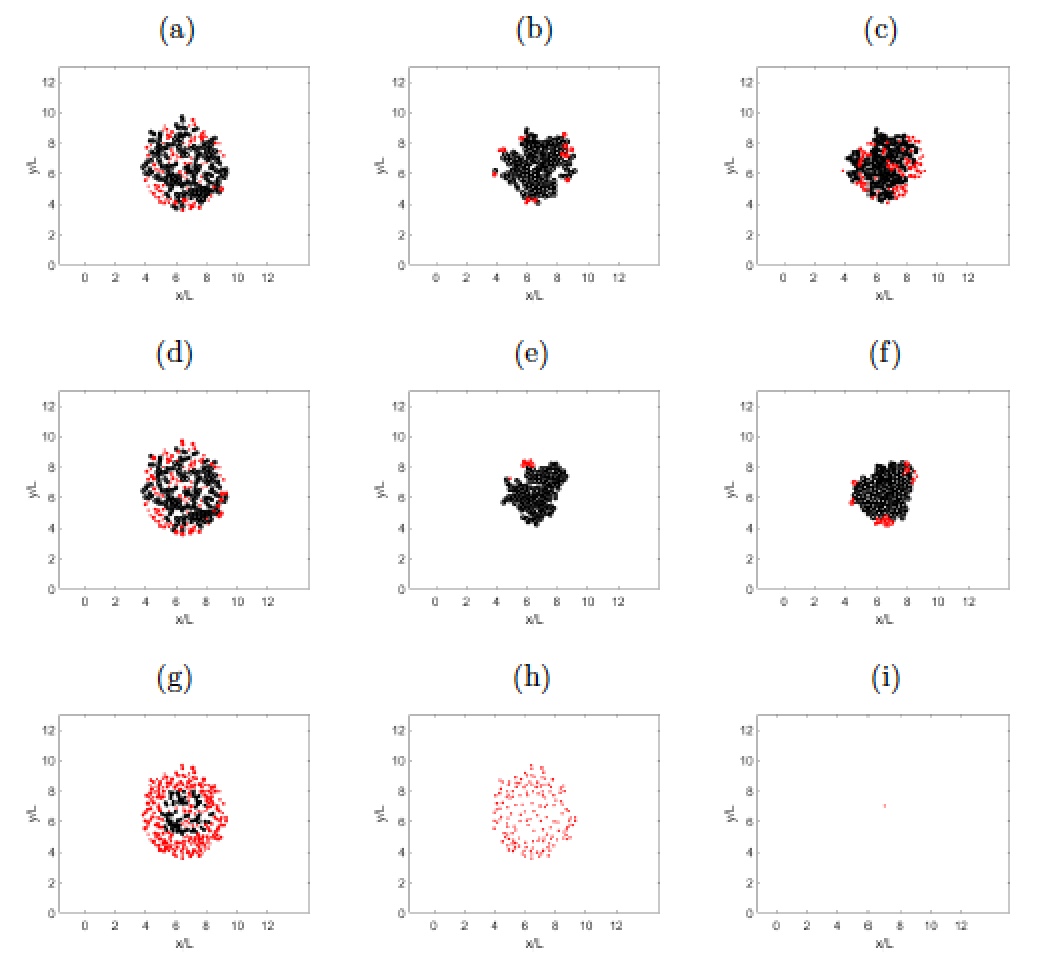
Figure 17: Equivalent of snapshots (a)-(c) and (d)-(f) with the modified death criterion: Snapshots for $C_{out}=3$ at (a) $t=2.5$ h, (a) $t=8.5$ h, and (c) $t=10$ h. The simulation ends with $184$ cells alive, $66$ dead (red) and $320$ erased, see Video7. Snapshots for $C_{out}=7$ at (d) $t=2.5$ h, (e) $t=8.5$ h, and (f) $t=10$ h with $141$ alive, The simulation ends with $20$ cells dead (red) and $327$ erased, see Video8. Finally, panels (g)-(i) represent the extinction of the same initial configuration with the modified death criterion and a combination of two antibiotics with $C_{out}=3$ and variable $k_{tox}$: (g) $t=2.5$ h, (h) $t=8.5$ h, and (i) $t=10$ h. The simulation ends with $0$ cells alive, $1$ dead (red) and $385$ erased, see Video9.

VII Conclusions

Studying the dynamics of cellular aggregates such as bacterial biofilms faces the challenge of dealing with complicated geometries and interactions. Many approaches have been proposed to that effect, with advantages and disadvantages. Cellular automata allow us to represent many microscopic and macroscopic processes Laspidou ; poroelastic , but ignore bacterial shapes and interactions. Individual based models seem effective for large biofilms growing in flows Picioreanu_fluids , but become exceedingly complicated for biofilms spreading on surfaces as the ones we consider here Picioreanu_surface ; Allen . Immersed boundary methods provide a very flexible alternative to study mechanical interactions in these complex geometries ibm_adhesion ; ibm_division ; ibm_tumor . Here, the immersed boundaries provide the basic geometrical skeleton, while the interaction with the medium is represented by forces governed by a set of equations coupling metabolic and physico-chemical processes. Cell growth, division, and death, is managed through additional rules on the evolution of the discrete boundaries. Unlike previous IB approaches to multicellular tissues, we do not include heuristical sources. Boundaries move as a result of cellular activity as dictated by a dynamic energy budget model, letting flow in and out through them. We have applied this framework to reproduce initial stages of the spread of a biofilm seed formed by a few spherical or rod-like bacteria in two dimensional geometries. Simulating rod-like bacteria is more expensive computationally. Computing the interactions of rods requires small steps to let configurations adapt as cells growth and divide avoiding overlaps. We observe that rod-like bacteria tend to align. In radial horizontal views, we see how crowded areas trigger the death of scattered bacteria, which are reabsorbed. For vertical slices expanding on an horizontal barrier, we see also gaps created by death bacteria near the barrier. In this case, we have implemented a mechanism to allow water flow inside the biofilm, so that gaps are filled with fluid and the separation between bacteria increases. When antibiotics are applied, bacteria located in the borders are first to die, forming small necrotic regions. We have shown that combining antibiotics which target either active or dormant cells within the layered biofilm structure we are able to drive the biofilm to complete extinction.

The specific results of the simulations depend on the parameters we choose. Most of parameters appearing in the model equations are taken from experimental measurements and fittings to population counts for some bacteria. However, there are a number of parameters in the representation of interaction forces, division and death criteria which are selected to produce adequate results, avoiding artifacts. Whether the whole set of parameters can be fitted to data counts for the time evolution of biofilm seeds of bacteria deserves further research. From a practical point of view, it would be important to be able to implement control strategies using the antibiotic supply as control variables to extinguish the whole biofilm seed in finite time.

- (1) E-address rafael09@ucm.es.
- (2) E-address ana_carpio@mat.ucm.es. Author to whom all correspondence should be addressed.
- (3) H.C. Flemming, J. Wingender, The biofilm matrix, Nat. Rev. Microbiol. 8, 623–633, 2010.
- (4) N. Høiby, T. Bjarnsholt, M. Givskov, S. Molin, O. Ciofu, Antibiotic resistance of bacterial biofilms, Int J Antimicrob Agents 35, 322–32, 2010.
- (5) K. Drescher, Y. Shen, B.L. Bassler, H.A. Stone, Biofilm streamers cause catastrophic disruption of flow with consequences for environmental and medical systems, Proc. Natl. Acad. Sci. USA 110, 4345–4350, 2013.
- (6) C. S. Laspidou, L. A. Spyrou, N. Aravas, B. E. Rittmann, Material modeling of biofilm mechanical properties, Math. Biosci. 251, 11-15, 2014.
- (7) L. A. Lardon, B. V. Merkey, S. Martins, A. Dötsch, C. Picioreanu, J. U. Kreft, B. F. Smets, iDynoMiCS: next-generation individual-based modelling of biofilms, Environ. Microbiol. 13, 2416-34, 2011.
- (8) R. Sudarsan, S. Ghosh, J.M. Stockie, H.J. Eberl, Simulating biofilm deformation and detachment with the immersed boundary method, Communications in Computational Physics 19, 682–732, 2016.
- (9) A. Seminara, T.E. Angelini, J.N. Wilking, H. Vlamakis, S. Ebrahim, R. Kolter, D.A. Weitz, M.P. Brenner, Osmotic spreading of Bacillus subtilis biofilms driven by an extracellular matrix, Proc. Natl. Acad. Sci. USA 109, 1116–1121, 2012.
- (10) T. Storck, C. Picioreanu, B. Virdis, D.J. Batstone, Variable cell morphology approach for individual-based modeling of microbial communities, Biophysical Journal 106, 2037–2048, 2014.
- (11) M. A. A. Grant, B.Waclaw, R. J. Allen, P. Cicuta, The role of mechanical forces in the planar-to-bulk transition in growing Escherichia coli microcolonies, J. R. Soc. Interface 11, 20140400, 2014.
- (12) A. Carpio, E. Cebrián, P. Vidal, Biofilms as poroelastic materials, International Journal of Non-Linear Mechanics 109, 1–8, 2019.
- (13) A. Carpio, E. Cebrián, Incorporating cellular stochasticity in solid-fluid mixture biofilm models, Entropy 22, 188, 2020.
- (14) R. Dillon, L. Fauci, A. Fogelson, D. Gaver, Modeling biofilm processes using the immersed boundary method, Journal of Computational Physics 129, 57–73, 1996.
- (15) J.A. Stotsky, J.F. Hammond, L. Pavlovsky, E.J. Stewart, J.G. Younger, M.J. Solomon, D.M. Bortz, Variable viscosity and density biofilm simulations using an immersed boundary method, Part II: Experimental validation and the heterogeneous rheology-IBM, Journal of Computational Physics 317, 204–222, 2016.
- (16) Y. Li, A. Yun, J. Kim, An immersed boundary method for simulating a single axisymmetric cell growth and division, Journal of Mathematical Biology 65, 653–675, 2012.
- (17) K.A. Rejniak, An immersed boundary framework for modelling the growth of individual cells: an application to the early tumour development, Journal of Theoretical Biology 247, 186–204, 2007.
- (18) R. Dillon, M. Owen, K. Painter, A single-cell-based model of multicellular growth using the immersed boundary method, In Moving Interface Problems and Applications in Fluid Dynamics (pp. 1–16). (Contemporary Mathematics). American Mathematical Society, 2008.
- (19) L. Chai, H. Vlamakis, R. Kolter, Extracellular signal regulation of cell differentiation in biofilms, MRS Bulletin 36, 374–379, 2011.
- (20) C.S. Peskin, D.M. McQueen, A general method for the computer simulation of biological systems interacting with fluids, Symposia of the Society for Experimental Biology 49, 265–76, 1995.
- (21) C.S. Peskin, The immersed boundary method, Acta Numerica 11, 479–517, 2002.
- (22) B. Birnir, A. Carpio, E. Cebrián, P. Vidal, Dynamic energy budget approach to evaluate antibiotic effects on biofilms, Commun Nonlinear Sci Numer Simulat 54, 70–83, 2018.
- (23) S.A.L.M. Kooijman, Dynamic energy budget theory for metabolic organization, Cambridge University Press 2008.
- (24) T. Klanjscek, R.M. Nisbet, J.H. Priester, P.A. Holden, Modeling physiological processes that relate toxicant exposure and bacterial population dynamics, PLoS One 7(2), e26955, 2012.
- (25) H.H. Tuson, G.K. Auer, L.D. Renner, M. Hasebe, C. Tropini, M. Salick, W.C. Crone, A. Gopinathan, K.C. Huang, D.B. Weibel, Measuring the stiffness of bacterial cells from growth rates in hydrogels of tunable elasticity, Mol Microbiol 84, 874–891, 2012.
- (26) K. Symon, Mechanics (Third edition), Addison-Wesley, 1971, ISBN 0-201-07392-7.