Abstract

We construct the diquark-diquark-diquark type vector six-quark currents to investigate the vector and scalar hexaquark states in the framework of the QCD sum rules in a consistent way, and make predictions for the hexaquark masses. We can search for the fully-heavy hexaquark states in the di-$\Omega_{ccc}$ and di-$\Omega_{bbb}$ invariant mass spectra in the future. Combined with our previous works on the fully-heavy tetraquark states and pentaquark states, the present predictions can shed light on the nature of the fully-heavy multiquark states.

PACS number: 12.39.Mk, 12.38.Lg

Key words: Fully-heavy hexaquark states, QCD sum rules

1 Introduction

In recent years, there has been great progress on the spectroscopy of the exotic states, which cannot find their suitable positions in the conventional spectra of the two-quark and three-quark models [1]. The exotic states provide us with an excellent subject to explore the strong interactions governing dynamics of the quarks and gluons, and confinement mechanism. It is interesting and necessary to explore the fully-heavy tetraquark (molecular) states, pentaquark (molecular) states and hexaquark (molecular) states, in those cases, we do not have to deal with the complex dynamics involving both explicit heavy and light degrees of freedoms.

Experimentally, in 2018, the LHCb collaboration investigated the $\Upsilon\,\mu^{+}\mu^{-}$ invariant-mass distribution for a possible exotic state $X_{bb\bar{b}\bar{b}}$ based on a data sample of proton-proton collisions recorded with the LHCb detector at $\sqrt{s}=7$, $8$ and $13\,\rm{TeV}$ corresponding to an integrated luminosity of ${\rm 6.3fb}^{-1}$, and observed no significant excess of events [2].

In 2020, the CMS collaboration searched for narrow resonances decaying to the final states $\Upsilon\,\mu^{+}\mu^{-}$ using proton-proton collision data collected in 2016 by the CMS experiment corresponding to an integrated luminosity of $35.9{\rm fb}^{-1}$, and observed no significant excess of events [3].

Also, in 2020, the LHCb collaboration observed a narrow structure $X(6900)$ and a broad structure just above the di-$J/\psi$ threshold in the di-$J/\psi$ invariant mass distributions with the statistical significance larger than $5\sigma$ using proton-proton collision data at center-of-mass energies of $\sqrt{s}=7$, $8$ and $13\,\rm{TeV}$ corresponding to an integrated luminosity of ${\rm 9fb}^{-1}$[4], such resonance structures are the first fully-heavy exotic multiquark candidates observed experimentally up to today.

The observation of the $X(6900)$ sheds some light on the nature of the exotic states and stimulates much interests in (and many works on) the fully-heavy multiquark states, such as the tetraquark (molecular) states, pentaquark (molecular) states, hexaquark (molecular) states, etc. There are four charm valence quarks considering its observation in the di-$J/\psi$ mass spectrum. The di-charmonium thresholds are $2M_{\eta_{c}}=5.968\,\rm{GeV}$, $2M_{J/\psi}=6.194\,\rm{GeV}$, $2M_{\chi_{c0}}=6.829\,\rm{GeV}$, $2M_{\chi_{c1}}=7.021$, $2M_{\chi_{c2}}=7.112\,\rm{GeV}$, $2M_{h_{c}}=7.051\,\rm{GeV}$ from the Particle Data Group [1], they lie either below or above the threshold of the $X(6900)$, it is difficult to assign the $X(6900)$ as the loosely bound tetraquark molecular state without introducing the (large) coupled-channel effects [5, 6, 7], it is more natural to assign the $X(6900)$ as the excited diquark-antidiquark type tetraquark state [8, 9, 10, 11, 12, 13, 14, 15, 16, 17, 18, 19, 20].

Usually, we expect that the loosely bound tetraquark molecular states have the spatial extension larger than $1\,\rm{fm}$. While in the QCD sum rules, we choose the local four-quark currents, which couple potentially to the compact color-singlet-color-singlet type tetraquark states, rather than to the loosely bound tetraquark molecular states, although we also call them as tetraquark molecular states in the QCD sum rules [21, 22].

The attractive force induced by one-gluon exchange favors forming the diquark correlations in color antitriplet, Fermi-Dirac statistics requires $\varepsilon^{abc}Q^{T}_{b}C\Gamma Q_{c}=\varepsilon^{abc}Q^{T}_{b}\left[C\Gamma\right]^{T}Q_{c}$, $\left[C\Gamma\right]^{T}=-C\Gamma$ for $\Gamma=\gamma_{5}$, $1$, $\gamma_{\mu}\gamma_{5}$; $\left[C\Gamma\right]^{T}=C\Gamma$ for $\Gamma=\gamma_{\mu}$, $\sigma_{\mu\nu}$, where the $a$, $b$ and $c$ are color indexes. Only the axialvector diquarks $\varepsilon^{abc}Q^{T}_{b}C\gamma_{\mu}Q_{c}$ and tensor diquarks $\varepsilon^{abc}Q^{T}_{b}C\sigma_{\mu\nu}Q_{c}$ can exist. The diquark operators $\varepsilon^{abc}Q^{T}_{b}C\sigma_{\mu\nu}Q_{c}$ have both the spin-parity $J^{P}=1^{+}$ and $1^{-}$ components, for the spin-parity $J^{P}=1^{-}$ component, there exists an implicit P-wave which is embodied in the negative parity, the axialvector diquark correlations are more stable than the tensor diquark correlations due to the additional energy excited by the P-wave. To obtain the lowest masses, we usually take the axialvector diquark operators $\varepsilon^{abc}Q^{T}_{b}C\gamma_{\mu}Q_{c}$ as the elementary constituents to explore the doubly-heavy (triply-heavy) baryon states, tetraquark states and pentaquark states [23, 24, 25, 26].

The tetraquark candidate $X(6900)$ was observed in the di-$J/\psi$ invariant mass spectrum [4], the pentaquark candidates $P_{c}(4312)$, $P_{c}(4380)$, $P_{c}(4440)$, $P_{c}(4457)$ were observed in the $J/\psi p$ invariant mass spectrum [27, 28]. Analogously, we expect to observe the fully-heavy pentaquark candidates $QQQQ\bar{Q}$ in the $J/\psi\Omega_{ccc}$ and $\Upsilon\Omega_{bbb}$ invariant mass spectra, expect to observe the fully-heavy hexaquark and dibaryon candidates $QQQQQQ$ in the $\Omega_{ccc}\Omega_{ccc}$ and $\Omega_{bbb}\Omega_{bbb}$ invariant mass spectra, expect to observe the fully-heavy baryonium candidates in the $\Omega_{ccc}\overline{\Omega}_{ccc}$ and $\Omega_{bbb}\overline{\Omega}_{bbb}$ invariant mass spectra at the LHCb, CEPC, FCC and ILC in the future.

Theoretically, there have been several works on the fully-heavy exotic states with more than four valence quarks. In Ref.[29], J. R. Zhang explores the color-singlet-color-singlet type $\eta_{c}\Omega_{ccc}$ and $\eta_{b}\Omega_{bbb}$ pentaquark molecular states with the QCD sum rules. In Ref.[30], we construct the diquark-diquark-antiquark type five-quark currents to study the fully-heavy pentaquark states in the framework of the QCD sum rules. In Ref.[31], H. T. An et al explore the fully-heavy pentaquark states with the modified chromo-magnetic interaction model .

As far as the hexaquark states are concerned, in Ref.[32], Y. Lyu et al study the dibaryon state $\Omega_{ccc}\Omega_{ccc}({}^{1}S_{0})$ based on the (2+1)-flavor lattice QCD and observe that there exists a shallow dibaryon state $\Omega_{ccc}\Omega_{ccc}({}^{1}S_{0})$ with the binding energy about $5.7\,\rm{MeV}$ and spatial extension about $\sqrt{\langle r^{2}\rangle}\approx 1.1\,\rm{fm}$. In Ref.[33], Liu and Geng explore the $\Omega\Omega$, $\Omega_{ccc}\Omega_{ccc}$ and $\Omega_{bbb}\Omega_{bbb}$ dibaryon states in the extended one-boson exchange model. In Ref.[34], H. Huang et al investigate the existence of the fully-heavy dibaryon states $\Omega_{ccc}\Omega_{bbb}$, $\Omega_{ccc}\Omega_{ccc}$ and $\Omega_{bbb}\Omega_{bbb}$ with the spins $J=0$, $1$, $2$, $3$ using a constituent quark model, and find that only the dibaryon state composed of six $c$ or $b$ quarks with the spin-parity $J^{P}=0^{+}$ can be bound. If there exist the $\Omega_{QQQ}\Omega_{QQQ}$ dibaryon states, naively, we expect that those color-singlet-color-singlet type hexaquark states lie below the di-$\Omega_{QQQ}$ thresholds, unfortunately, the triply-heavy baryon states still escape the experimental detections up to today [23].

In previous works, we constructed the color-singlet-color-singlet type (color-singlet-color-singlet-color-singlet type) six-quark currents to explore the triply-heavy dibaryon (hexaquark molecular) states and doubly-heavy dibaryon states with the QCD sum rules [35, 36, 37] ([38]), and constructed the diquark-diquark-diquark type six-quark currents to explore the triply-heavy hexaquark state with the QCD sum rules [39]. In all the works [35, 36, 37, 38, 39], there are explicit light degrees of freedoms in the six-quark currents, the contributions from the valence light quarks are very large.

In this work, we construct the diquark-diquark-diquark type local six-quark currents to study the fully-heavy hexaquark states with the spin-parity $J^{P}=1^{-}$ and $0^{+}$ consistently in the framework of the QCD sum rules, and make predictions for the hexaquark masses to be confronted to the experimental data in the future, because the QCD sum rules approach is a powerful theoretical tool in studying the exotic $X$, $Y$, $Z$ and $P$ states [40].

The article is arranged as follows: in Sect.2, we acquire the QCD sum rules for the fully-heavy hexaquark states; in Sect.3, we present the numerical results and discussions; Sect.4 is reserved for our conclusion.

2 QCD sum rules for the fully-heavy hexaquark states

Firstly, we write down the correlation functions $\Pi_{\mu\nu}(p)$,

$$\Pi_{\mu\nu}(p) = i\int d^{4}xe^{ip\cdot x}\langle 0|T\left\{J_{\mu}(x)J_{\nu}^{\dagger}(0)\right\}|0\rangle\,,$$ (1)

where

$$J_{\mu}(x) = \varepsilon^{ijk}\varepsilon_{\mu\nu\alpha\beta}\,A^{\nu}_{i}(x)\,A_{j}^{\alpha}(x)\,A^{\beta}_{k}(x)\,,$$

$$A_{i}^{\mu}(x) = \varepsilon^{ijk}Q^{T}_{j}(x)C\gamma^{\mu}Q_{k}(x)\,,$$ (2)

$Q=b$, $c$, the $i$, $j$, $k$ are color indexes. We can construct other diquark-diquark-diquark type six-quark currents consisting of the same flavor to interpolate the fully-heavy hexaquark states,

$$\eta_{\mu}{}^{\nu^{\prime}\alpha^{\prime}\beta^{\prime}}(x) = \varepsilon^{ijk}\varepsilon_{\mu\nu\alpha\beta}\,T^{\nu\nu^{\prime}}_{i}(x)\,T_{j}^{\alpha\alpha^{\prime}}(x)\,T^{\beta\beta^{\prime}}_{k}(x)+\cdots\,,$$

$$T_{i}^{\mu\nu}(x) = \varepsilon^{ijk}Q^{T}_{j}(x)C\sigma^{\mu\nu}Q_{k}(x)\,,$$ (3)

where the Lorentz indexes $\nu^{\prime}$, $\alpha^{\prime}$, $\beta^{\prime}$ are symmetric. The tensor diquark operators $T_{i}^{\mu\nu}(x)$ have both the spin-parity $J^{P}=1^{+}$ and $1^{-}$ components, the P-wave effect is embodied in the negative parity, the additional P-wave leads to less stable tensor diquark correlations compared to the axialvector diquark correlations. Therefore, the currents $\eta_{\mu}{}^{\nu^{\prime}\alpha^{\prime}\beta^{\prime}}(x)$ couple potentially to the fully-heavy hexaquark states with much (or slightly) larger masses than that of the currents $J_{\mu}(x)$.

Under parity transform $\widehat{P}$, the currents $J_{\mu}(x)$ have the property,

$$\widehat{P}J_{i}(x)\widehat{P}^{-1} = -J_{i}(\tilde{x})\,,$$

$$\widehat{P}J_{0}(x)\widehat{P}^{-1} = +J_{0}(\tilde{x})\,,$$ (4)

where $x^{\mu}=(t,\vec{x})$ and $\tilde{x}^{\mu}=(t,-\vec{x})$. The currents $J_{\mu}(x)$ couple potentially to both the vector and scalar fully-heavy hexaquark states, the correlation functions $\Pi_{\mu\nu}(p)$ at the hadron side can be written as,

$$\Pi_{\mu\nu}(p) = \frac{\lambda_{V}^{2}}{M_{V}^{2}-p^{2}}\left(-g_{\mu\nu}+\frac{p_{\mu}p_{\nu}}{p^{2}}\right)+\frac{\lambda_{S}^{2}}{M_{S}^{2}-p^{2}}\frac{p_{\mu}p_{\nu}}{p^{2}}+\cdots\,,$$ (5)

$$= \Pi_{V}(p^{2})\left(-g_{\mu\nu}+\frac{p_{\mu}p_{\nu}}{p^{2}}\right)+\Pi_{S}(p^{2})\frac{p_{\mu}p_{\nu}}{p^{2}}\,,$$

where the pole residues $\lambda_{V}$ and $\lambda_{S}$ are defined by,

$$\langle 0|J_{\mu}(0)|V(p)\rangle = \lambda_{V}\,\varepsilon_{\mu}\,,$$

$$\langle 0|J_{\mu}(0)|S(p)\rangle = \lambda_{S}\,\frac{p_{\mu}}{\sqrt{p^{2}}}\,,$$ (6)

the $\varepsilon_{\mu}$ are the polarization vectors of the vector fully-heavy hexaquark states.

We accomplish the tedious and terrible operator product expansion and take account of the gluon condensates, then obtain the spectral densities $\frac{{\rm Im\,\Pi}_{V/S}(s)}{\pi}$ at the quark level through dispersion relation,

$$\Pi_{V/S}(p^{2}) = \frac{1}{\pi}\int_{36m_{Q}^{2}}^{\infty}ds\frac{{\rm Im\,\Pi}_{V/S}(s)}{s-p^{2}}\,.$$ (7)

We match the hadron side with the QCD side of the correlation functions $\Pi_{V/S}(p^{2})$ below the continuum thresholds $s_{0}$ and perform the Borel transform with respect to the $P^{2}=-p^{2}$ to obtain the QCD sum rules:

$$\lambda_{V/S}^{2}\exp\left(-\frac{M_{V/S}^{2}}{T^{2}}\right) = \int_{36m_{Q}^{2}}^{s_{0}}ds\int_{16m_{Q}^{2}}^{(\sqrt{s}-2m_{Q})^{2}}dr\int_{4m_{Q}^{2}}^{(\sqrt{r}-2m_{Q})^{2}}dt_{1}\int_{4m_{Q}^{2}}^{(\sqrt{r}-\sqrt{t_{1}})^{2}}dt_{2}\int_{4m_{Q}^{2}}^{(\sqrt{s}-\sqrt{r})^{2}}dt_{3}$$ (8)

$$\rho_{V/S}(s,r,t_{1},t_{2},t_{3})\exp\left(-\frac{s}{T^{2}}\right)\,,$$

where

$$\rho_{V/S} = \frac{\sqrt{\lambda(s,r,t_{3})}}{s}\frac{\sqrt{\lambda(r,t_{1},t_{2})}}{r}\frac{\sqrt{\lambda(t_{1},m_{Q}^{2},m_{Q}^{2})}}{t_{1}}\frac{\sqrt{\lambda(t_{2},m_{Q}^{2},m_{Q}^{2})}}{t_{2}}\frac{\sqrt{\lambda(t_{3},m_{Q}^{2},m_{Q}^{2})}}{t_{3}}$$ (9)

$$\left(C_{V/S,4}\,m_{Q}^{4}+C_{V/S,2}\,m_{Q}^{2}+C_{V/S,0}\right)$$

$$+\langle\frac{\alpha_{s}GG}{\pi}\rangle\frac{\sqrt{\lambda(s,r,t_{3})}}{s}\frac{\sqrt{\lambda(r,t_{1},t_{2})}}{r}\frac{\sqrt{\lambda(t_{1},m_{Q}^{2},m_{Q}^{2})}}{t_{1}}\frac{\sqrt{\lambda(t_{2},m_{Q}^{2},m_{Q}^{2})}}{t_{2}}$$

$$\frac{1}{t_{3}\sqrt{\lambda(t_{3},m_{Q}^{2},m_{Q}^{2})}^{5}}\left(C^{gg}_{V/S,10}\,m_{Q}^{10}+C_{V/S,8}^{gg}\,m_{Q}^{8}+C_{V/S,6}^{gg}\,m_{Q}^{6}+C_{V/S,4}^{gg}\,m_{Q}^{4}+C_{V/S,2}^{gg}m_{Q}^{2}\right)$$

$$+\langle\frac{\alpha_{s}GG}{\pi}\rangle\frac{\sqrt{\lambda(s,r,t_{3})}}{s}\frac{\sqrt{\lambda(r,t_{1},t_{2})}}{r}\frac{\sqrt{\lambda(t_{1},m_{Q}^{2},m_{Q}^{2})}}{t_{1}}\frac{\sqrt{\lambda(t_{2},m_{Q}^{2},m_{Q}^{2})}}{t_{2}}$$

$$\frac{1}{t_{3}\sqrt{\lambda(t_{3},m_{Q}^{2},m_{Q}^{2})}^{3}}\left(C_{V/S,8}^{g-g}\,m_{Q}^{8}+C_{V/S,6}^{g-g}\,m_{Q}^{6}+C_{V/S,4}^{g-g}\,m_{Q}^{4}+C_{V/S,2}^{g-g}m_{Q}^{2}\right)\,,$$

$\lambda(a,b,c)=a^{2}+b^{2}+c^{2}-2ab-2bc-2ac$, the $T^{2}$ is the Borel parameter, the lengthy/cumbersome expressions of the coefficients $C_{V/S,4}$, $C_{V/S,2}$, $C_{V/S,0}$, $C^{gg}_{V/S,10}$, $C_{V/S,8}^{gg}$, $C_{V/S,6}^{gg}$, $C_{V/S,4}^{gg}$, $C_{V/S,2}^{gg}$, $C_{V/S,8}^{g-g}$, $C_{V/S,6}^{g-g}$, $C_{V/S,4}^{g-g}$, $C_{V/S,2}^{g-g}$ are neglected for simplicity, the interested readers can get them in the Fortran form through contacting me via E-mail. In the following, we give an example to illustrate the function forms of the coefficients,

$$C_{S,0} = \frac{3}{512\pi^{10}}\left[t_{2}t_{3}(t_{2}+t_{3})-t_{1}t_{3}(t_{1}+t_{3})-9t_{1}t_{2}(r+t_{3})+\frac{t_{3}}{2}(s+r)(t_{1}-t_{2})+\frac{9st_{1}t_{2}}{2}\right.$$ (10)

$$-\frac{st_{3}}{r}(t_{1}^{2}-t_{2}^{2})+\frac{2t_{3}^{2}}{r}(t_{1}^{2}-t_{2}^{2})-\frac{9rt_{1}t_{2}t_{3}}{s}+\frac{rt_{2}t_{3}}{s}(t_{2}+t_{3})+\frac{2t_{3}^{2}}{s}(t_{1}^{2}-t_{2}^{2})-\frac{rt_{1}t_{3}}{s}(t_{1}+t_{3})$$

$$-\frac{3t_{1}t_{2}t_{3}}{2r}(t_{1}-t_{2})+\frac{t_{3}}{2r}(t_{1}^{3}-t_{2}^{3})+\frac{9t_{1}t_{2}}{2s}(r^{2}+t_{3}^{2})-\frac{3t_{1}t_{2}t_{3}}{2s}(t_{1}-t_{2})+\frac{r^{2}t_{3}}{2s}(t_{1}-t_{2})$$

$$+\frac{t_{1}t_{3}}{2s}(t_{1}^{2}+t_{3}^{2})-\frac{t_{2}t_{3}}{2s}(t_{2}^{2}+t_{3}^{2})+\frac{3t_{1}t_{2}t_{3}^{2}}{rs}(t_{1}-t_{2})+\frac{t_{2}^{2}t_{3}^{2}}{sr}(t_{2}+t_{3})-\frac{t_{1}^{2}t_{3}^{2}}{rs}(t_{1}+t_{3})$$

$$+\frac{3t_{1}t_{2}t_{3}^{2}}{r^{2}}(t_{1}-t_{2})-\frac{t_{1}^{2}t_{3}^{2}}{r^{2}}(t_{1}-t_{3})-\frac{3st_{1}t_{2}t_{3}}{2r^{2}}(t_{1}-t_{2})+\frac{st_{3}}{2r^{2}}(t_{1}^{3}-t_{2}^{3})+\frac{t_{3}^{3}}{2r^{2}s}(t_{1}^{3}-t_{2}^{3})$$

$$\left.-\frac{3t_{1}t_{2}t_{3}^{3}}{2r^{2}s}(t_{1}-t_{2})\right]\,.$$

It is the most simple coefficient, the total expressions of all the coefficients will cost more pages than the whole text. The superscripts $gg$ and $g-g$ in the coefficients $C^{gg}_{V/S,10}$, $C_{V/S,8}^{gg}$, $\cdots$, $C_{V/S,8}^{g-g}$, $C_{V/S,6}^{g-g}$, $\cdots$ correspond to the Feynman diagrams where the two gluons which form the gluon condensates are emitted from one heavy-quark line (the first Feynman diagram in Fig.1) and two heavy-quark lines (the second Feynman diagram in Fig.1), respectively. In calculations, we expand the QCD spectral densities $\rho_{V/S}(s,r,t_{1},t_{2},t_{3})$ in terms of the powers of the $m_{Q}^{2}$, such as $m_{Q}^{0}$, $m_{Q}^{2}$, $m_{Q}^{4}$, $m_{Q}^{6}$, $\cdots$, the coefficients $C_{V/S,4}$, $C_{V/S,2}$, $C_{V/S,0}$, $C^{gg}_{V/S,10}$, $\cdots$ are functions of the variables $s$, $r$, $t_{1}$, $t_{2}$ and $t_{3}$, just like that shown in Eq.(10). There are end-point divergences $\frac{1}{\sqrt{t_{3}-4m_{Q}^{2}}^{5}}$ and $\frac{1}{\sqrt{t_{3}-4m_{Q}^{2}}^{3}}$ because $\lambda(t_{3},m_{Q}^{2},m_{Q}^{2})=t_{3}\left(t_{3}-4m_{Q}^{2}\right)$, the end-point divergence $\frac{1}{\sqrt{t_{3}-4m_{Q}^{2}}^{5}}$ is much worse than the end-point divergence $\frac{1}{\sqrt{t_{3}-4m_{Q}^{2}}^{3}}$, we regulate the divergences by adding a uniform mass term $\Delta^{2}$ in the divergent terms $\frac{1}{\sqrt{t_{3}-4m_{Q}^{2}+\Delta^{2}}^{5}}$ and $\frac{1}{\sqrt{t_{3}-4m_{Q}^{2}+\Delta^{2}}^{3}}$ with the value $\Delta^{2}=m_{Q}^{2}$ [30]. In the Appendix, we illustrate how to calculate the Feynman diagrams and illustrate the origins of the end-point divergences. The three-gluon condensate makes tiny contribution in the Borel windows for the triply-heavy baryon states [23], such a tendency survives for the fully-heavy exotic multiquark states. We neglect the three-gluon condensate, as it is the vacuum expectation value of the gluon operators of the order $\mathcal{O}(\alpha_{s}^{k})$ with $k=\frac{3}{2}$ [41, 42, 43, 44]. Direct calculations indicate that the vacuum condensates which are vacuum expectation values of the quark-gluon operators of the order $\mathcal{O}(\alpha_{s}^{k})$ with $\frac{3}{2}\leq k\leq 3$ can be neglected safely [36].

Figure 1: The Feynman diagrams make contributions to the gluon condensates. Other Feynman diagrams obtained by interchanging of the $Q$ quark lines are implied.

We differentiate Eq.(8) in regard to $\frac{1}{T^{2}}$, then eliminate the pole residues $\lambda_{V/S}$ and obtain the masses for the vector and scalar fully-heavy hexaquark states,

$$M^{2}_{V/S} = -\frac{\frac{d}{d(1/T^{2})}\int_{36m_{Q}^{2}}^{s_{0}}ds\,\rho_{V/S;QCD}(s)\exp\left(-\frac{s}{T^{2}}\right)}{\int_{36m_{Q}^{2}}^{s_{0}}ds\,\rho_{V/S;QCD}(s)\exp\left(-\frac{s}{T^{2}}\right)}\,,$$ (11)

where the $\rho_{V/S;QCD}(s)$ are the corresponding spectral densities.

3 Numerical results and discussions

We choose the gluon condensate $\langle\frac{\alpha_{s}GG}{\pi}\rangle=0.012\pm 0.004\,\rm{GeV}^{4}$ [45, 46, 47], and take the $\overline{MS}$ masses of the heavy quarks $m_{c}(m_{c})=(1.275\pm 0.025)\,\rm{GeV}$ and $m_{b}(m_{b})=(4.18\pm 0.03)\,\rm{GeV}$ from the Particle Data Group [1]. All the nonperturbative dynamics and confinement effects are embodied in the running heavy quark masses and vacuum condensates, we take account of the energy-scale dependence of the $\overline{MS}$ masses,

$$m_{Q}(\mu) = m_{Q}(m_{Q})\left[\frac{\alpha_{s}(\mu)}{\alpha_{s}(m_{Q})}\right]^{\frac{12}{33-2n_{f}}}\,,$$

$$\alpha_{s}(\mu) = \frac{1}{b_{0}t}\left[1-\frac{b_{1}}{b_{0}^{2}}\frac{\log t}{t}+\frac{b_{1}^{2}(\log^{2}{t}-\log{t}-1)+b_{0}b_{2}}{b_{0}^{4}t^{2}}\right]\,,$$ (12)

where $t=\log\frac{\mu^{2}}{\Lambda^{2}}$, $b_{0}=\frac{33-2n_{f}}{12\pi}$, $b_{1}=\frac{153-19n_{f}}{24\pi^{2}}$, $b_{2}=\frac{2857-\frac{5033}{9}n_{f}+\frac{325}{27}n_{f}^{2}}{128\pi^{3}}$, $\Lambda=213\,\rm{MeV}$, $296\,\rm{MeV}$ and $339\,\rm{MeV}$ for the quark flavor numbers $n_{f}=5$, $4$ and $3$, respectively [1]. We choose the flavors $n_{f}=4$ and $5$ for the fully-heavy hexaquark states $cccccc$ and $bbbbbb$, respectively, and then evolve the heavy quark masses to the typical energy scales $\mu=m_{c}(m_{c})$ (i.e. $1.275\,\rm{GeV}$) and $2.8\,\rm{GeV}$ to extract the masses of the hexaquark states $cccccc$ and $bbbbbb$, respectively, just like in our previous work on the fully-heavy pentaquark states [30], and add an uncertainty $\delta\mu=\pm 0.1\,\rm{GeV}$ [30, 38]. Furthermore, we present the predictions based on the updated gluon condensate obtained by S. Narison, $\langle\frac{\alpha_{s}GG}{\pi}\rangle=0.021\pm 0.001\,\rm{GeV}^{4}$ [48].

We should choose suitable continuum thresholds $s_{0}$ to avoid contaminations from the first radial excited states and continuum states. In previous works, we choose $\sqrt{s_{0}}=M_{B}+0.50\sim 0.55\pm 0.10\,\rm{GeV}$ for the triply-heavy baryon states $B$ [23], $\sqrt{s_{0}}=M_{X}+0.50\pm 0.10\,\rm{GeV}$ for the fully-heavy tetraquark states $X$ [24, 25], $\sqrt{s_{0}}=M_{X/Z}+0.55\pm 0.10\,\rm{GeV}$ for the hidden-charm and hidden-bottom tetraquark states $X_{Q}$ and $Z_{Q}$ [41, 42], $\sqrt{s_{0}}=M_{P}+0.65\pm 0.10\,\rm{GeV}$ for the hidden-charm pentaquark states $P_{c}$ and $P_{cs}$ [43, 44], $\sqrt{s_{0}}=M_{P}+0.60\pm 0.10\,\rm{GeV}$ for the fully-heavy pentaquark states $P_{Q}$ [30]. To obtain the lowest hexaquark masses, we prefer the smaller continuum threshold parameters and require the continuum threshold parameters satisfy the relation $\sqrt{s_{0}}=M_{V/S}+0.50\pm 0.10\,\rm{GeV}$ tentatively, and change the Borel parameters and continuum threshold parameters to acquire the best values via trial and error. We tentatively choose a continuum threshold parameter $s_{0}$, then obtain the numerical value of the hexaquark mass $M_{V/S}$ from the QCD sum rules, and judge whether or not the two basic criteria of the QCD sum rules (plus the constraint $\sqrt{s_{0}}=M_{V/S}+0.5\pm 0.1\,\rm{GeV}$) are satisfied. If not, we choose another continuum threshold parameter $s_{0}$ until reach the satisfactory results.

At last, we obtain the best continuum threshold parameters, Borel parameters, and pole contributions, which are shown explicitly in Table 1. In the Borel windows, the pole contributions are about $(40-60)\%$, the pole dominance criterion is satisfied. On the other hand, the main contributions come from the perturbative terms, the gluon condensate contributions play a minor role, and change slowly with variations of the Borel parameters, the convergent behaviors of the operator product expansion are very good. In the Borel windows, the contributions of the gluon condensate are about $-2\%$ ($-4\%$) and $-1\%$ ($-2\%$) for the $J^{P}=1^{-}$ and $0^{+}$ fully-charm hexaquark states, respectively, and $\ll 1\%$ for the $J^{P}=1^{-}$ and $0^{+}$ fully-bottom hexaquark states, where the values in the brackets come from the updated gluon condensate [48]. We choose the Borel windows with the help of the uniform pole contributions $(40-60)\%$, as the convergence of the operator product expansion is almost warranted automatically.

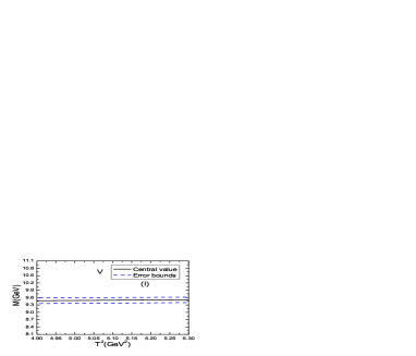
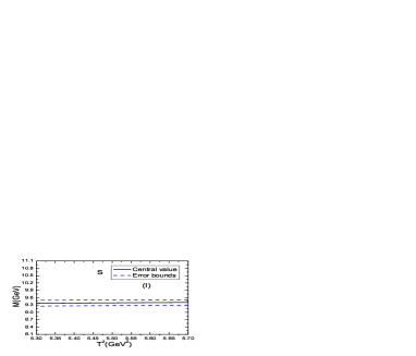
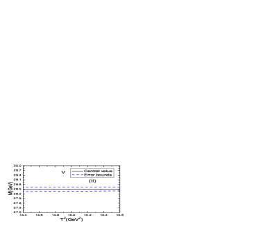
We take account of all uncertainties of the relevant parameters, and acquire the masses and pole residues of the fully-heavy hexaquark states, which are also shown plainly in Table 1 and Fig.2. In Table 1, we also present the values of the masses and pole residues acquired with the updated gluon condensate obtained by S. Narison [48]. From the Table, we can see clearly that the standard values and updated values lead to in-distinguishable predictions, which emerge as a result of the tiny contributions of the gluon condensate. From Fig.2, we can see that there appear very flat platforms for the hexaquark masses, the uncertainties come from the Borel parameters are rather small, the predictions are robust.

In calculations, we observe that the masses and pole residues increase monotonously and slowly with the increase of the continuum threshold parameters, we determine the continuum threshold parameters $s_{0}$ by adopting the uniform constraints, such as the continuum thresholds $\sqrt{s_{0}}=M_{V/S}+0.50\pm 0.1\,\rm{GeV}$, pole contributions $(40\sim 60)\%$ and intervals $T^{2}_{max}-T^{2}_{min}=0.4\,\rm{GeV}^{2}$ ($1.2\,\rm{GeV}^{2}$) to acquire reliable predictions for the hexaquark states $cccccc$ ($bbbbbb$), where the $T^{2}_{max}$ and $T^{2}_{min}$ stand for the maximum and minimum values of the Borel platforms, respectively.

	$J^{P}$	$T^{2}(\rm{GeV}^{2})$	$\sqrt{s_{0}}(\rm GeV)$	pole	$M(\rm GeV)$	$\lambda(\rm GeV^{8})$
$cccccc$	$1^{-}$	$4.9-5.3$	$10.00\pm 0.10$	$(41-61)\%$	$9.49\pm 0.13$	$(1.03\pm 0.43)\times 10^{-1}$
					$9.50\pm 0.13$	$(1.03\pm 0.43)\times 10^{-1}$
$cccccc$	$0^{+}$	$5.3-5.7$	$9.90\pm 0.10$	$(41-59)\%$	$9.39\pm 0.13$	$(3.37\pm 1.21)\times 10^{-1}$
					$9.39\pm 0.13$	$(3.36\pm 1.21)\times 10^{-1}$
$bbbbbb$	$1^{-}$	$14.4-15.6$	$29.00\pm 0.10$	$(40-60)\%$	$28.50\pm 0.15$	$5.61\pm 2.70$
					$28.50\pm 0.15$	$5.61\pm 2.70$
$bbbbbb$	$0^{+}$	$15.6-16.8$	$28.90\pm 0.10$	$(41-59)\%$	$28.39\pm 0.15$	$35.3\pm 15.6$
					$28.39\pm 0.15$	$35.3\pm 15.6$

Table 1: The Borel parameters, continuum threshold parameters, pole contributions, masses and pole residues for the ground state fully-heavy hexaquark states, the values in the lower lines are obtained from the updated gluon condensate.

Figure 2: The masses of the vector ($V$) and scalar ($S$) hexaquark states with variations of the Borel parameters $T^{2}$, where the (I) and (II) denote the $cccccc$ and $bbbbbb$ hexaquark states, respectively.

The thresholds of the tri-$J/\psi$, tri-$\eta_{c}$, tri-$\Upsilon$ and tri-$\eta_{b}$ are $3M_{J/\psi}=9.291\,\rm{GeV}$, $3M_{\eta_{c}}=8.952\,\rm{GeV}$, $3M_{\Upsilon}=28.381\,\rm{GeV}$ and $3M_{\eta_{b}}=28.196\,\rm{GeV}$ respectively from the Particle Data Group [1], the central values have the relations,

$$M_{cccccc}(1^{-}) > M_{cccccc}(0^{+})>3M_{J/\psi}>3M_{\eta_{c}}\,,$$

$$M_{bbbbbb}(1^{-}) > M_{bbbbbb}(0^{+})>3M_{\Upsilon}>3M_{\eta_{b}}\,.$$ (13)

The fully-heavy hexaquark states $QQQQQQ$ have net positive or negative electric charges, naively, we expect that the repulsive electromagnetic interactions between the heavy quarks $Q$ and $Q$ lead to larger spatial extended bound states that of the heavy quark pairs $Q$ and $\bar{Q}$, where the attractive electromagnetic interactions always favor forming tighter bound states, it is natural that the ground state masses have the relations $M_{cccccc}(0^{+})\geq 3M_{J/\psi}$ and $M_{bbbbbb}(0^{+})\geq 3M_{\Upsilon}$. There exist an additional P-wave in the vector fully-heavy hexaquark states, which can excite some additional energies, so the masses have the hierarchies $M_{cccccc}(1^{-})\geq M_{cccccc}(0^{+})$ and $M_{bbbbbb}(1^{-})\geq M_{bbbbbb}(0^{+})$, the predictions are reasonable.

The decays of the fully-heavy hexaquark states can take place through the Okubo-Zweig-Iizuka super-allowed fall-apart mechanism,

$$cccccc\,(1^{-},0^{+}) \to \Omega_{ccc}\,\Omega_{ccc}\,,$$

$$bbbbbb\,(1^{-},0^{+}) \to \Omega_{bbb}\,\Omega_{bbb}\,,$$ (14)

if there are enough phase-spaces. According to the recent analysis of the QCD sum rules [23], $M_{\Omega(ccc)}=4.81\pm 0.10\,\rm{GeV}$ and $M_{\Omega(bbb)}=14.43\pm 0.09\,\rm{GeV}$, we obtain the relations,

$$M_{cccccc}(0^{+}) \leq M_{cccccc}(1^{-})\leq 2M_{\Omega(ccc)}=9.62\pm 0.20\,\rm{GeV}\,,$$

$$M_{bbbbbb}(0^{+}) \leq M_{bbbbbb}(1^{-})\leq 2M_{\Omega(bbb)}=28.86\pm 0.18\,\rm{GeV}\,,$$ (15)

there only exist rather small phase-spaces due to uncertainties, the decays are kinematically suppressed. In other words, the decays can take place through the intermediate virtual $\Omega_{ccc}^{*}$ and $\Omega_{bbb}^{*}$ states,

$$cccccc\,(1^{-},0^{+}) \to \Omega_{ccc}\,\Omega_{ccc}^{*}\,,$$

$$bbbbbb\,(1^{-},0^{+}) \to \Omega_{bbb}\,\Omega_{bbb}^{*}\,.$$ (16)

In Ref.[32], the studies based on the (2+1)-flavor lattice QCD indicate that the dibaryon state $\Omega_{ccc}\Omega_{ccc}({}^{1}S_{0})$ has the binding energy about $5.7\,\rm{MeV}$, i.e. it lies about $5.7\,\rm{MeV}$ below the di-$\Omega_{ccc}$ threshold, which is consistent with the present calculations, as a hadron maybe have several Fock components, we can choose several currents to interpolate it. Experimentally, we can search for the fully-heavy hexaquark states in the di-$\Omega_{ccc}$ and di-$\Omega_{bbb}$ invariant mass spectra at the LHCb, CEPC, FCC and ILC in the future.

Unfortunately, up to now, the triply-heavy baryon states $\Omega_{ccc}$ and $\Omega_{bbb}$ still escape from experimental detections, and we can search for them in the decay chains, $\Omega_{ccc}\to\Omega_{ccs}\,\pi^{+}\to\Omega_{css}\,\pi^{+}\pi^{+}\to\Omega_{sss}\,\pi^{+}\pi^{+}\pi^{+}$ and $\Omega_{bbb}\to\Omega_{bbs}\,J/\psi\to\Omega_{bss}\,J/\psi J/\psi\to\Omega_{sss}\,J/\psi J/\psi J/\psi$ through the weak decays $c\to su\bar{d}$ and $b\to c\bar{c}s$ at the quark level. We can search for the doubly/singly-heavy baryon states $\Omega_{ccs}({\frac{1}{2}}^{+})$, $\Omega_{ccs}({\frac{3}{2}}^{+})$, $\Omega_{bbs}({\frac{1}{2}}^{+})$, $\Omega_{bbs}({\frac{3}{2}}^{+})$ and $\Omega_{bss}({\frac{3}{2}}^{+})$ as a byproduct and additional benefit, as they have not been observed yet.

4 Conclusion

In this article, we extend our previous works on the fully-heavy baryon states, tetraquark states and pentaquark states to explore the fully-heavy hexaquark states, and construct the diquark-diquark-diquark type vector local six-quark currents to study the vector and scalar hexaquark states consistently in the framework of the QCD sum rules. After accomplishing the tedious calculations, we obtain the masses and pole residues of the fully-heavy hexaquark states. The central values of the predicted hexaquark masses $M_{cccccc}(1^{-})=9.49\pm 0.13\,\rm{GeV}$, $M_{cccccc}(0^{+})=9.39\pm 0.13\,\rm{GeV}$, $M_{bbbbbb}(1^{-})=28.50\pm 0.15\,\rm{GeV}$, $M_{bbbbbb}(0^{+})=28.39\pm 0.15\,\rm{GeV}$ lies slightly below the corresponding di-$\Omega_{ccc}$ and di-$\Omega_{bbb}$ thresholds, respectively, if we choose the masses of the $\Omega_{QQQ}$ states from the recent analysis of the QCD sum rules as the input parameters, the strong decays to the di-$\Omega_{ccc}$ and di-$\Omega_{bbb}$ induced states can take place through the intermediate virtual $\Omega_{ccc}^{*}$ and $\Omega_{bbb}^{*}$ states. We should bear in mind that the decays to the di-$\Omega_{QQQ}$ states are not forbidden due to the uncertainties. We can search for the fully-heavy hexaquark states in the di-$\Omega_{ccc}$ and di-$\Omega_{bbb}$ invariant mass spectra at the LHCb, CEPC, FCC and ILC in the future, and confront the predictions to the experimental data.

Appendix

Now we illustrate how to accomplish the operator product expansion, at the lowest order,

$$\Pi_{\mu\nu}(p) = \int d^{4}k_{1}d^{4}k_{2}d^{4}k_{3}d^{4}k_{4}d^{4}k_{5}d^{4}k_{6}\,\delta^{4}\left(p-k_{1}-k_{2}-k_{3}-k_{4}-k_{5}-k_{6}\right)$$ (17)

$$\frac{f_{\mu\nu}(k_{1},k_{2},k_{3},k_{4},k_{5},k_{6})}{\left(k_{1}^{2}-m_{Q}^{2}\right)\left(k_{2}^{2}-m_{Q}^{2}\right)\left(k_{3}^{2}-m_{Q}^{2}\right)\left(k_{4}^{2}-m_{Q}^{2}\right)\left(k_{5}^{2}-m_{Q}^{2}\right)\left(k_{6}^{2}-m_{Q}^{2}\right)}\,,$$

$$= \int d^{4}q_{1}d^{4}q_{2}d^{4}q_{3}\,\delta^{4}\left(p-q_{1}-q_{2}-q_{3}\right)$$

$$\frac{(-2\pi i)^{2}}{2\pi i}\int_{4m_{Q}^{2}}^{t_{1}^{f}}dt_{1}\frac{1}{t_{1}-q_{1}^{2}}\int d^{4}k_{1}d^{4}k_{2}\,\delta^{4}\left(q_{1}-k_{1}-k_{2}\right)\delta\left(k_{1}^{2}-m_{Q}^{2}\right)\delta\left(k_{2}^{2}-m_{Q}^{2}\right)$$

$$\frac{(-2\pi i)^{2}}{2\pi i}\int_{4m_{Q}^{2}}^{t_{2}^{f}}dt_{2}\frac{1}{t_{2}-q_{2}^{2}}\int d^{4}k_{3}d^{4}k_{4}\,\delta^{4}\left(q_{2}-k_{3}-k_{4}\right)\delta\left(k_{3}^{2}-m_{Q}^{2}\right)\delta\left(k_{4}^{2}-m_{Q}^{2}\right)$$

$$\frac{(-2\pi i)^{2}}{2\pi i}\int_{4m_{Q}^{2}}^{t_{3}^{f}}dt_{3}\frac{1}{t_{3}-q_{3}^{2}}\int d^{4}k_{5}d^{4}k_{6}\,\delta^{4}\left(q_{3}-k_{5}-k_{6}\right)\delta\left(k_{5}^{2}-m_{Q}^{2}\right)\delta\left(k_{6}^{2}-m_{Q}^{2}\right)$$

$$f_{\mu\nu}(k_{1},k_{2},k_{3},k_{4},k_{5},k_{6})\,,$$

where the $f_{\mu\nu}(k_{1},k_{2},k_{3},k_{4},k_{5},k_{6})$ denotes the numerator after carrying out the trace in the Dirac spinor space, the $t_{1}^{f}$, $t_{2}^{f}$ and $t_{3}^{f}$ are the upper bounds of the integrals. Then we accomplish the integrals $\int d^{4}k_{1}d^{4}k_{2}$, $\int d^{4}k_{3}d^{4}k_{4}$ and $\int d^{4}k_{5}d^{4}k_{6}$ to obtain,

$$\Pi_{\mu\nu}(p) = \int d^{4}p_{1}d^{4}q_{3}\,\delta^{4}\left(p-p_{1}-q_{3}\right)$$

$$\frac{(-2\pi i)^{2}}{2\pi i}\int_{16m_{Q}^{2}}^{r^{f}}dr\frac{1}{r-p_{1}^{2}}\int_{4m_{Q}^{2}}^{t_{1}^{f}}dt_{1}\int_{4m_{Q}^{2}}^{t_{2}^{f}}dt_{2}\int_{4m_{Q}^{2}}^{t_{3}^{f}}dt_{3}$$

$$\int d^{4}q_{1}d^{4}q_{2}\,\delta^{4}\left(p_{1}-q_{1}-q_{2}\right)\delta\left(q_{1}^{2}-t_{1}\right)\delta\left(q_{2}^{2}-t_{2}\right)\frac{1}{t_{3}-q_{3}^{2}}\,\tilde{f}_{\mu\nu}(q_{1},q_{2},q_{3},t_{1},t_{2},t_{3})$$

$$= \frac{(-2\pi i)^{2}}{2\pi i}\int_{36m_{Q}^{2}}^{\infty}ds\frac{1}{s-p^{2}}\int_{16m_{Q}^{2}}^{r^{f}}dr\int_{4m_{Q}^{2}}^{t_{1}^{f}}dt_{1}\int_{4m_{Q}^{2}}^{t_{2}^{f}}dt_{2}\int_{4m_{Q}^{2}}^{t_{3}^{f}}dt_{3}$$

$$\int d^{4}p_{1}d^{4}q_{3}\,\delta^{4}\left(p-p_{1}-q_{3}\right)\delta\left(p_{1}^{2}-r\right)\delta\left(q_{3}^{2}-t_{3}\right)$$

$$\frac{(-2\pi i)^{2}}{2\pi i}\int d^{4}q_{1}d^{4}q_{2}\,\delta^{4}\left(p_{1}-q_{1}-q_{2}\right)\delta\left(q_{1}^{2}-t_{1}\right)\delta\left(q_{2}^{2}-t_{2}\right)\,\tilde{f}_{\mu\nu}(q_{1},q_{2},q_{3},t_{1},t_{2},t_{3})\,,$$

where the $\tilde{f}_{\mu\nu}(q_{1},q_{2},q_{3},t_{1},t_{2},t_{3})$ denotes the lengthy expressions after accomplishing the integrals $\int d^{4}k_{1}d^{4}k_{2}$, $\int d^{4}k_{3}d^{4}k_{4}$ and $\int d^{4}k_{5}d^{4}k_{6}$, the $r^{f}$ is the upper bound of the integral. Finally, we accomplish the integrals $\int d^{4}p_{1}d^{4}q_{3}$ and $\int d^{4}q_{1}d^{4}q_{2}$ to obtain,

$$\Pi_{\mu\nu}(p) = \int_{36m_{Q}^{2}}^{s_{0}}ds\int_{16m_{Q}^{2}}^{(\sqrt{s}-2m_{Q})^{2}}dr\int_{4m_{Q}^{2}}^{(\sqrt{r}-2m_{Q})^{2}}dt_{1}\int_{4m_{Q}^{2}}^{(\sqrt{r}-\sqrt{t_{1}})^{2}}dt_{2}\int_{4m_{Q}^{2}}^{(\sqrt{s}-\sqrt{r})^{2}}dt_{3}$$

$$\frac{1}{s-p^{2}}\left\{\rho_{V}(s,r,t_{1},t_{2},t_{3})\left(-g_{\mu\nu}+\frac{p_{\mu}p_{\nu}}{p^{2}}\right)+\rho_{S}(s,r,t_{1},t_{2},t_{3})\frac{p_{\mu}p_{\nu}}{p^{2}}\right\}+\cdots\,.$$

Now we give an example to illustrate the endpoint divergence, at the lowest order, we often encounter the typical integral,

$$I_{11} = \int d^{4}k_{1}d^{4}k_{2}\frac{1}{k_{1}^{2}-m_{1}^{2}}\frac{1}{k_{2}^{2}-m_{2}^{2}}\delta^{4}\left(q-k_{1}-k_{2}\right)\,,$$ (20)

and calculate it by using the Cutkosky’s rules,

$$I_{11} = \frac{(-2\pi i)^{2}}{2\pi i}\int_{(m_{1}+m_{2})^{2}}^{\infty}dt\frac{1}{t-q^{2}}\int d^{4}k_{1}d^{4}k_{2}\delta^{4}(q-k_{1}-k_{2})\delta(k_{1}^{2}-m_{1}^{2})\delta(k_{2}^{2}-m_{2}^{2})$$ (21)

$$= \frac{(-2\pi i)^{2}}{2\pi i}\int_{(m_{1}+m_{2})^{2}}^{\infty}dt\frac{1}{t-q^{2}}\frac{\pi}{2}\frac{\sqrt{\lambda(t,m_{1}^{2},m_{2}^{2})}}{t}\,,$$

which is free of end-point divergence. At the second Feynman diagram in Fig.1, we often encounter the typical integral,

$$I_{22} = \int d^{4}k_{1}d^{4}k_{2}\frac{1}{(k_{1}^{2}-m_{1}^{2})^{2}}\frac{1}{(k_{2}^{2}-m_{2}^{2})^{2}}\delta^{4}\left(q-k_{1}-k_{2}\right)\,,$$ (22)

again we calculate it by using the Cutkosky’s rules,

$$I_{22} = \frac{\partial^{2}}{\partial A\partial B}\int d^{4}k_{1}d^{4}k_{2}\frac{1}{k_{1}^{2}-A}\frac{1}{k_{2}^{2}-B}\delta^{4}\left(q-k_{1}-k_{2}\right)\mid_{A\to m_{1}^{2};B\to m_{2}^{2}}$$ (23)

$$= \frac{\partial^{2}}{\partial A\partial B}\frac{(-2\pi i)^{2}}{2\pi i}\int_{(\sqrt{A}+\sqrt{B})^{2}}^{\infty}dt\frac{1}{t-q^{2}}\int d^{4}k_{1}d^{4}k_{2}\delta^{4}(q-k_{1}-k_{2})\delta(k_{1}^{2}-A)\delta(k_{2}^{2}-B)$$

$$= \frac{\partial^{2}}{\partial A\partial B}\frac{(-2\pi i)^{2}}{2\pi i}\int_{(\sqrt{A}+\sqrt{B})^{2}}^{\infty}dt\frac{1}{t-q^{2}}\frac{\pi}{2}\frac{\sqrt{\lambda(t,A,B)}}{t}$$

$$= \frac{(-2\pi i)^{2}}{2\pi i}\int_{(m_{1}+m_{2})^{2}}^{\infty}dt\frac{1}{t-q^{2}}\frac{\pi}{2}\frac{2(m_{1}^{2}+m_{2}^{2}-t)}{\sqrt{\lambda(t,m_{1}^{2},m_{2}^{2})}^{3}}\,.$$

In the limit $m_{1}^{2}=m_{2}^{2}=m_{Q}^{2}$, we obtain

$$\int_{(m_{1}+m_{2})^{2}}^{\infty}dt\frac{1}{t-q^{2}}\frac{1}{\sqrt{\lambda(t,m_{1}^{2},m_{2}^{2})}^{3}} = \int_{4m_{Q}^{2}}^{\infty}dt\frac{1}{t-q^{2}}\frac{1}{\sqrt{t(t-4m_{Q}^{2})}^{3}}\,,$$ (24)

divergence at the end-point $t=4m_{Q}^{2}$. For the end-point divergence $\frac{1}{\sqrt{t-4m_{Q}^{2}}^{5}}$ appears at the first diagram in Fig.1, the calculations are analogous. The end-point divergences appear as a natural outcome of the calculations using the Cutkosky’s rules, and are usually regularized by adding a mass term.

References

- [1] P. A. Zyla et al, Prog. Theor. Exp. Phys. 2020 (2020) 083C01.
- [2] R. Aaij et al, JHEP 10 (2018) 086.
- [3] A. Sirunyan et al, Phys. Lett. B 808 (2020) 135578.
- [4] R. Aaij et al, Sci. Bull. 65 (2020) 1983.
- [5] X. K. Dong, V. Baru, F. K. Guo, C. Hanhart and A. Nefediev, Phys. Rev. Lett. 127 (2021) 119901.
- [6] Z. H. Guo and J. A. Oller, Phys. Rev. D103 (2021) 034024.
- [7] Q. F. Cao, H. Chen, H. R. Qi and H. Q. Zheng, Chin. Phys. C45 (2021) 103102.
- [8] Z. G. Wang, Chin. Phys. C44 (2020) 113106.
- [9] M. A. Bedolla, J. Ferretti, C. D. Roberts and E. Santopinto, Eur. Phys. J. C80 (2020) 1004.
- [10] Q. F. Lu, D. Y. Chen and Y. B. Dong, Eur. Phys. J. C80 (2020) 871.
- [11] J. F. Giron and R. F. Lebed, Phys. Rev. D102 (2020) 074003.
- [12] M. Karliner and J. L. Rosner, Phys. Rev. D102 (2020) 114039.
- [13] X. Z. Weng, X. L. Chen, W. Z. Deng and S. L. Zhu, Phys. Rev. D103 (2021) 034001.
- [14] C. Deng, H. Chen and J. Ping, Phys. Rev. D103 (2021) 014001.
- [15] X. Jin, Y. Xue, H. Huang and J. Ping, Eur. Phys. J. C80 (2020) 1083.
- [16] C. Becchi, J. Ferretti, A. Giachino, L. Maiani and E. Santopinto, Phys. Lett. B811 (2020) 135952.
- [17] J. Sonnenschein and D. Weissman, Eur. Phys. J. C81 (2021) 25.
- [18] K. T. Chao and S. L. Zhu, Sci. Bull. 65 (2020) 1952.
- [19] R. N. Faustov, V. O. Galkin and E. M. Savchenko, Phys. Rev. D102 (2020) 114030.
- [20] R. Zhu, Nucl. Phys. B966 (2021) 115393.
- [21] Z. G. Wang, Adv. High Energy Phys. 2021 (2021) 4426163.
- [22] Z. G. Wang, arXiv:2102.07520 [hep-ph].
- [23] Z. G. Wang, AAPPS Bull. 31 (2021) 5.
- [24] Z. G. Wang, Eur. Phys. J. C77 (2017) 432.
- [25] Z. G. Wang and Z. Y. Di, Acta Phys. Polon. B50 (2019) 1335.
- [26] Z. G. Wang, Eur. Phys. J. C78 (2018) 826.
- [27] R. Aaij et al, Phys. Rev. Lett. 115 (2015) 072001.
- [28] R. Aaij et al, Phys. Rev. Lett. 122 (2019) 222001.
- [29] J. R. Zhang, Phys. Rev. D103 (2021) 074016.
- [30] Z. G. Wang, Nucl. Phys. B973 (2021) 115579.
- [31] H. T. An, K. Chen, Z. W. Liu and X. Liu, Phys. Rev. D 103 (2021) 074006.
- [32] Y. Lyu et al, Phys. Rev. Lett. 127 (2021) 072003.
- [33] M. Z. Liu and L. S. Geng, Chin. Phys. Lett. 38 (2021) 101201.
- [34] H. Huang, J. Ping, X. Zhu and F. Wang, arXiv:2011.00513.
- [35] Z. G. Wang, Phys. Rev. D102 (2020) 034008.
- [36] X. W. Wang, Z. G. Wang and G. L. Yu, Eur. Phys. J. A57 (2021) 275.
- [37] X. W. Wang and Z. G. Wang, Adv. High Energy Phys. 2022 (2022) 6224597.
- [38] Z. G. Wang, Commun. Theor. Phys. 73 (2021) 065201.
- [39] Z. G. Wang, Int. J. Mod. Phys. A35 (2020) 2050073.
- [40] R. M. Albuquerque et al, J. Phys. G46 (2019) 093002.
- [41] Z. G. Wang, Eur. Phys. J. C79 (2019) 489.
- [42] Z. G. Wang, Phys. Rev. D102 (2020) 014018.
- [43] Z. G. Wang, Int. J. Mod. Phys. A35 (2020) 2050003.
- [44] Z. G. Wang, Int. J. Mod. Phys. A36 (2021) 2150071.
- [45] M. A. Shifman, A. I. Vainshtein and V. I. Zakharov, Nucl. Phys. B147 (1979) 385, 448.
- [46] L. J. Reinders, H. Rubinstein and S. Yazaki, Phys. Rept. 127 (1985) 1.
- [47] P. Colangelo and A. Khodjamirian, hep-ph/0010175.
- [48] S. Narison, Nucl. Part. Phys. Proc. 312-317 (2021) 87.