Evolution of short-period cataclysmic variables: implications from eclipse
modeling and stage A superhump method (with New Year’s gift)
Abstract
In 2013, the method of determining mass ratios () of dwarf novae using stage A superhumps (growing superhumps) was established. This method is a dynamical one in that it relies only on celestial mechanics. It is not dependent on an experimental calibration. Since then, more than 100 objects have been measured by this method and this method have also been applied to AM CVn stars and a black-hole X-ray binary, but these achievements have often been neglected. In this paper, I provide an updated description of the method. Comparisons with the results of the modern eclipse modeling method, which is considered to be the golden standard, have shown that these two methods agree very well and I have confirmed that the stage A superhump method is as accurate and as reliable as the modern eclipse modeling method. The stage A superhump method has many points advantageous over the eclipse modeling method in that the former does not require large telescopes and can be applicable to non-eclipsing systems. The number of objects determined by the stage A superhump method is now a few times of that by the modern eclipse modeling and they are now indispensable to study the terminal evolution of cataclysmic variables. I also showed that past studies by the other groups assumed incorrect fractional superhump excess ()- relations, causing biases in discussing the evolution. In particular, formulae given in Patterson (2001) and Patterson et al. (2005a) should be avoided. I derived a new experimental - relation of stage B superhumps and showed that the pressure effect during stage B of superhumps has an only weak dependence on . I derived a refined evolutionary track around the period minimum suggesting that the angular momentum loss is 1.9 times larger than what is expected by gravitational wave radiation. The period minimum on this track occurs at 0.0562 d = 81.0 min. There is a sharp peak in the distribution of the mass of the secondaries around the period minimum. The values rule out the claimed existence of very low-mass white dwarfs () among dwarf novae below the period gap. The measurements of stage A superhumps greatly owe to international collaborations with amateurs and professionals. I describe a brief summary of these collaborations and highlight the similarity with the world of birding (or ornithology) in that they play a role in uniting the world via international exchanges of observations. I also describe my thoughts about the similarity and relation between astronomy and ornithology, and give prospects how multidisciplinary works can be made possible between these seemingly distant fields of science.
tkato@kusastro.kyoto-u.ac.jp
(Abstract is given at the end of the paper).
Prologue
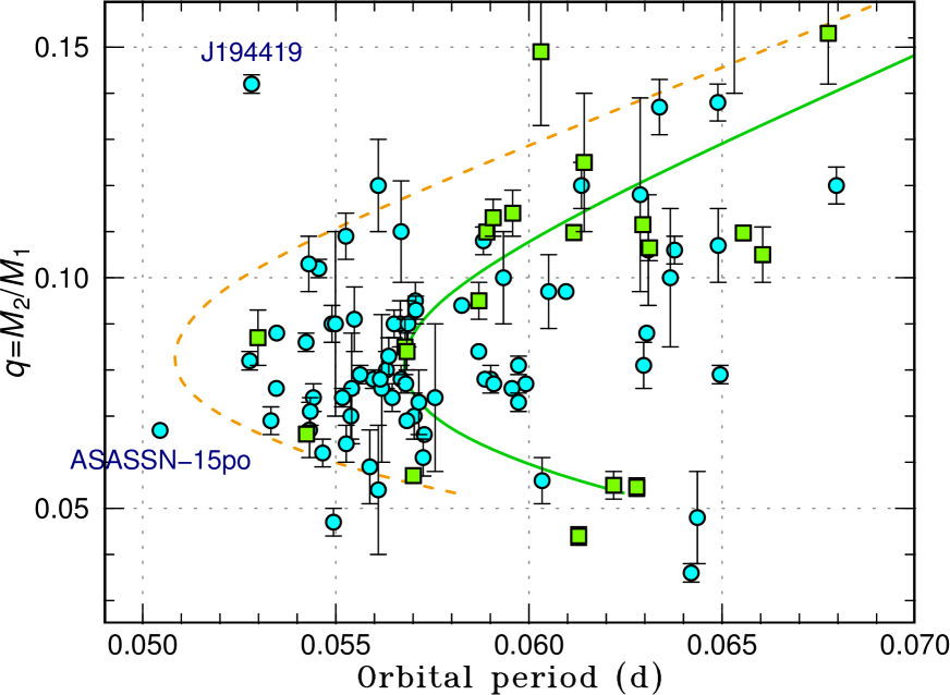
“Look to the skies, and you will feel it — a deep universal fascination …” — stargazers will completely agree with the phrase, but this is the beginning of the narration of the TV documentary “Extraordinary Birds” directed by Tom Simon in 2000. I refrain from talking about my favorite birds for a while; now, just look at figure 1! Although this may not be as fascinating as what you see in the skies, this is a figure summarizing our current best knowledge about the terminal evolution of cataclysmic variables (CVs). CVs are close binaries consisting of a white dwarf and a mass-transferring low-mass dwarf star. CVs evolve from upper right on this figure from long orbital periods () to shorter and to lower mass ratios () by transferring the matter from the secondary. CVs then reach the “period minimum”, after which lengthens while is still decreasing. Such objects are called “period bouncers”.
This figure contains two symbols representing measurements by two state-of-the-art methods to determine . One method employs 3.5–8.2 m telescopes equipped with a specially designed multicolor high-speed camera (there were even Nature and Science papers among them: Littlefair et al. (2006); Hernández Santisteban et al. (2016)). The other employs 20–50 cm telescopes, which are often owned by amateur astronomers equipped with off-the-shelf CCD cameras. Can you tell which symbol is which?
This question would be difficult to answer: these two methods give almost the same results and mutually reinforce the reliability each other. In other words, the second method (stage A superhump method) is as reliable as the first method (eclipse modeling). I will explain the reason in the following sections. If you are interested to contribute to observations by the second method, a book “Cataclysmic Variable Stars: How and why they vary” by Hellier (2001) will be helpful. Our Variable Star Network team (VSNET Collaboration: Kato et al. (2004)) regularly receive observations of superhumps from amateurs and professionals worldwide and your observations will surely contribute to reveal the secrets of CVs.
It is a pity, however, that the measurements of by the stage A superhump method tend to be neglected by researchers of the CV evolution, probably due to a persistent misunderstanding that the reliability of superhumps for determining is limited partly because it is dependent on experimental calibration based on old knowledge before the 2010s. In this paper, I review the history of the misunderstanding, the current reliable method and a comparison with the results of the eclipse modeling method using a high-speed photometer, which is usually considered to be most accurate.
1 Historical Development
Superhumps in SU UMa-type dwarf novae have periods (superhump period, ) a few percent longer than the orbital period [for general information of cataclysmic variables and dwarf novae, see e.g. Warner (1995)]. Superhumps are widely accepted to be caused by a precessing eccentric accretion disk which arises from the 3:1 resonance (Whitehurst 1988; Hirose and Osaki 1990; Lubow 1991). The presence of the gravity of the secondary star causes the deviation of the gravitational field from the inverse square law by the white dwarf primary [see e.g. Hirose and Osaki (1990) for a mathematical treatment], it is natural to consider that the precession rate () can be used as a measure of the binary mass ratio , where and are the masses of the primary (white dwarf) and the secondary which transfers matter to the primary, respectively. The relation between , and is:
| (1) |
where is the orbital angular frequency of the binary. In actual observations, the fractional superhump excess () is widely used:
| (2) |
The relation between and is:
| (3) |
The fractional superhump excesses were, however, historically only used to derive approximate values of mainly due to the two reasons:
-
(1)
The precession rate depends on the radius or the mass distribution of the disk, which is usually difficult to determine by observations.
-
(2)
The precession rate usually does not reflect the purely dynamical precession. The pressure effect slows down the precession rate. (Lubow 1992; Hirose and Osaki 1993; Murray 1998; Montgomery 2001; Pearson 2006), while the pressure effect is difficult to formulate (see e.g. Montgomery (2001); Pearson (2006)) or measure by observations.
Before the identification of the nature of superhumps, Stolz and Schoembs (1984) made a pioneering work illustrating that there is a linear relation between and . This relation was updated by Robinson et al. (1987). This Stolz-Schoembs relation has widely been used to estimate from (e.g. Ritter (1984)). This relation also implied that should be a strong function of following the evolution of cataclysmic variables (Warner 1976; Patterson 1984). Molnar and Kobulnicky (1992) first systematically studied the relation between and , and then . They found very good linear relations between and , and between and assuming main-sequence secondaries. This Molnar-Kobulnicky relation was used to estimate from or (such as Howell et al. (1993); Kato et al. (2001)). Lemm et al. (1993); Skillman and Patterson (1993); Leibowitz et al. (1994) presented updated figures of the Molnar-Kobulnicky relation. The work by Mineshige et al. (1992) was one of the first to directly estimate from . They introduced , the ratio between the disk radius and the radius of the 3:1 resonance, and estimated from measurements of SU UMa stars and applied to superhumps in black-hole X-ray transients to estimate the masses of the black holes. This empirical calibration, however, was not widely used by researchers of cataclysmic variables [I could only find Retter et al. (1997)].
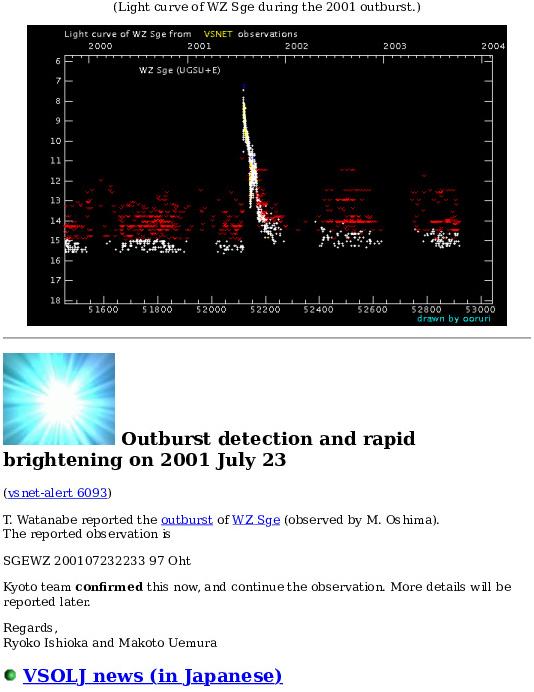
An independent effort to calibrate the - relation became necessary following an burst of new detections of superhumps in WZ Sge stars [the examples being HV Vir in 1992: Leibowitz et al. (1994); Kato et al. (2001), AL Com in 1995: Pych and Olech (1995); Kato et al. (1996); Howell et al. (1996); Patterson et al. (1996); Nogami et al. (1997), EG Cnc in 1996: Patterson et al. (1998); Kato et al. (2004), V2176 Cyg in 1997: Novák et al. (2001); Kwast and Semeniuk (1998), V592 Her in 1998: Duerbeck and Mennickent (1998); Kato et al. (2002), WZ Sge in 2001: Patterson et al. (2002); Ishioka et al. (2002); Baba et al. (2002), figure 2; see Kato (2015) for a modern review of WZ Sge stars]. These WZ Sge stars drew attention of researchers since they have very low-mass secondaries which may be brown dwarfs. Patterson (1998) derived an equation
| (4) |
combined with the analytical formula of the precession rate. Patterson (2001) further calibrated the relation using observed superhump excesses and obtained
| (5) |
This relation was derived from various classes of objects ranging from dwarf novae to novalike variables and X-ray binaries. Patterson et al. (2005a) published a refinement of the empirical relation
| (6) |
based on a broader sample of objects ranging from dwarf novae to novalike variables. In Patterson (2001), only one X-ray binary (KV UMa) was used in contrast to Patterson (2001). These three formulae are still most widely used. These “Patterson” relations, however, have intrinsic difficulties. In addition to the reasons listed earlier in this section, there are difficulties:
-
(3)
The pressure effect is expected to be different depending on the state of the accretion disk (see e.g. Pearson (2006)). Patterson’s calibration relied on different states: non-stationary outbursting dwarf novae, steady state novalike disks and an X-ray binaries, which can have disk sizes and temperatures different from CVs and contributions of the pressure effect may be different.
-
(4)
Patterson’s formulae assumed =0 at =0, which is incorrect if the pressure effect is taken into account.
According to Lubow (1992), the (apsidal) precession rate can be written as a form:
| (7) |
where the first term, , represents a contribution to disk precession due to the gravitational potential of the secondary, giving rise to prograde precession, the second term, (negative value), the pressure effect giving rise to retrograde precession, and the last term, , the minor wave-wave interaction. The functional form of is given in the next section. As one could naturally see, is small when is small. is, however, not very dependent on and the effect of this term can become larger than that of the first term for very small . This is the reason why the item (4) is important. The same issue was also pointed out by Goodchild and Ogilvie (2006).
2 Modern Method Using Stage A Superhumps
2.1 Superhumps and dynamical precession
The situation has changed since the identification of superhump stages (stages A, B and C: Kato et al. (2009a)). Kato et al. (2009a) showed that the periods of superhumps systematically vary. Stage A superhumps appear first when superhumps grow. It was not certain at that time which stage is suitable for estimating . In Kato and Osaki (2013), however, stage A superhumps were identified to reflect the dynamical precession rate of the disk at the radius of the 3:1 resonance. Stage B superhumps with smaller is most strongly affected by the pressure effect and was found to be inadequate to derive [Patterson’s formulae used stage B superhumps for dwarf novae; see footnote 11 in Patterson (2011)]. Following the treatment in Kato and Osaki (2013),111 The equations in this part are not absolutely necessary to understand the stage A superhump method and its applications. One can skip this part and proceed to the next section if necessary.
| (8) |
is the dimensionless radius measured in units of the binary separation . The dependence on and can be described as (cf. Hirose and Osaki (1990))
| (9) |
and
| (10) |
where is the Laplace coefficient222 Please don’t be discouraged by a formula with an integral. Modern computer languages have functions for numerical integrations and this integral can be very quickly computed.
| (11) |
There is also a polynomial expression (Pearson 2003, 2006):
| (12) |
where
| (13) |
The full polynomial formula for the dynamical precession rate can be written down as
| (14) |
The convergence of this formula is rather slow and it requires 12–13 terms (i.e. up to or ) to obtain a precision of 10-6 around the radius the 3:1 resonance.
2.2 Stage A superhumps and mass ratio
During stage A, it is considered that the superhump wave is confined to the 3:1 resonance region and the the pressure effect can be neglected [see figure 13 in Osaki and Kato (2013) or figure 4 in Niijima et al. (2021) for schematic representations of the pressure effect and the regions of the superhump wave]. One can substitute by the radius of the 3:1 resonance.
| (15) |
Then becomes a function of and we can directly estimate from of stage A superhumps.
Originally in Kato and Osaki (2013), the equations (8) to (10) were combined and described as
| (16) |
There was a typo introduced while writing down an equation in LaTeX in equation (16) = equation (1) in Kato and Osaki (2013), and the correction was made in Kato et al. (2016c). The correct equation is
| (17) |
The same incorrect equation was written in Kato et al. (2013b), Nakata et al. (2013) and Kato (2015). The figure and table dealing with this equation in Kato and Osaki (2013) were correct. No published values by the stage A superhump method were affected by this typo.
The stage A superhump method is a dynamical method to determine in that it relies only on celestial mechanics. The equation is analytical and no experimental calibration is needed. These features are clearly advantageous over the classical superhump methods such as the Patterson relations. For users’ convenience for interpolation, I provide an extended version of table 1 and figure 2 in Kato and Osaki (2013) in table 2.2 and figure 3. Note that the values are given for (probably) unrealistic values of . There is also a polynomial expression of this relation [equation (7) in Warner (1995) = equation (3.41b) in Warner (1995)]:
| (18) |
I have confirmed that this equation (up to this term) gives the same value in table 2.2 to a precision of 0.001 in . Although there is also a polynomial equation (4) in Kato and Osaki (2013), please do not cite this equation since it is a regression, not an analytical formula.
| 0.000 | 0.0000 | 0.024 | 0.0636 | 0.048 | 0.1395 | 0.072 | 0.2322 | 0.096 | 0.3482 |
|---|---|---|---|---|---|---|---|---|---|
| 0.001 | 0.0024 | 0.025 | 0.0665 | 0.049 | 0.1430 | 0.073 | 0.2365 | 0.097 | 0.3537 |
| 0.002 | 0.0049 | 0.026 | 0.0694 | 0.050 | 0.1465 | 0.074 | 0.2409 | 0.098 | 0.3592 |
| 0.003 | 0.0074 | 0.027 | 0.0723 | 0.051 | 0.1501 | 0.075 | 0.2453 | 0.099 | 0.3648 |
| 0.004 | 0.0099 | 0.028 | 0.0753 | 0.052 | 0.1537 | 0.076 | 0.2497 | 0.100 | 0.3705 |
| 0.005 | 0.0124 | 0.029 | 0.0782 | 0.053 | 0.1573 | 0.077 | 0.2542 | 0.101 | 0.3762 |
| 0.006 | 0.0149 | 0.030 | 0.0813 | 0.054 | 0.1609 | 0.078 | 0.2587 | 0.102 | 0.3820 |
| 0.007 | 0.0174 | 0.031 | 0.0843 | 0.055 | 0.1646 | 0.079 | 0.2633 | 0.103 | 0.3879 |
| 0.008 | 0.0200 | 0.032 | 0.0873 | 0.056 | 0.1683 | 0.080 | 0.2679 | 0.104 | 0.3938 |
| 0.009 | 0.0226 | 0.033 | 0.0904 | 0.057 | 0.1720 | 0.081 | 0.2725 | 0.105 | 0.3998 |
| 0.010 | 0.0252 | 0.034 | 0.0935 | 0.058 | 0.1758 | 0.082 | 0.2772 | 0.106 | 0.4058 |
| 0.011 | 0.0278 | 0.035 | 0.0966 | 0.059 | 0.1796 | 0.083 | 0.2820 | 0.107 | 0.4119 |
| 0.012 | 0.0304 | 0.036 | 0.0998 | 0.060 | 0.1834 | 0.084 | 0.2868 | 0.108 | 0.4181 |
| 0.013 | 0.0331 | 0.037 | 0.1029 | 0.061 | 0.1873 | 0.085 | 0.2916 | 0.109 | 0.4244 |
| 0.014 | 0.0358 | 0.038 | 0.1061 | 0.062 | 0.1912 | 0.086 | 0.2965 | 0.110 | 0.4307 |
| 0.015 | 0.0385 | 0.039 | 0.1094 | 0.063 | 0.1951 | 0.087 | 0.3014 | 0.111 | 0.4371 |
| 0.016 | 0.0412 | 0.040 | 0.1126 | 0.064 | 0.1991 | 0.088 | 0.3064 | 0.112 | 0.4436 |
| 0.017 | 0.0439 | 0.041 | 0.1159 | 0.065 | 0.2031 | 0.089 | 0.3114 | 0.113 | 0.4502 |
| 0.018 | 0.0466 | 0.042 | 0.1192 | 0.066 | 0.2072 | 0.090 | 0.3165 | 0.114 | 0.4568 |
| 0.019 | 0.0494 | 0.043 | 0.1225 | 0.067 | 0.2112 | 0.091 | 0.3217 | 0.115 | 0.4635 |
| 0.020 | 0.0522 | 0.044 | 0.1258 | 0.068 | 0.2154 | 0.092 | 0.3269 | 0.116 | 0.4703 |
| 0.021 | 0.0550 | 0.045 | 0.1292 | 0.069 | 0.2195 | 0.093 | 0.3321 | 0.117 | 0.4772 |
| 0.022 | 0.0578 | 0.046 | 0.1326 | 0.070 | 0.2237 | 0.094 | 0.3374 | 0.118 | 0.4842 |
| 0.023 | 0.0607 | 0.047 | 0.1361 | 0.071 | 0.2279 | 0.095 | 0.3428 | 0.119 | 0.4912 |
This stage A superhump method has been applied to many SU UMa and WZ Sge stars, such as in a series of papers Kato et al. (2014b)–Kato et al. (2020). At the time of writing of the present paper, values have been determined by the stage A superhump method for more than 100 objects. There have been indirect estimations of values using Kato and Osaki (2013), such as a combination of the periods of stage A superhumps and post-superoutburst superhumps (Kato et al. 2013b, 2019).
2.3 Relation between stage B superhump period and mass ratio
Using the empirical relation between fractional superhump excesses of stage A and stage B superhumps [equation (9) in Kato and Osaki (2013)]:
| (19) |
where is the expected precession rate at the 3:1 resonance. This indirect method is helpful when the periods of stage A superhumps are unknown but uncertainties resulting from an experimental calibration remain (the problem of =0 at =0 in Patterson’s formulae is, however, avoided). Examples of applications of this method can be found in Pavlenko et al. (2021); Shugarov et al. (2021). These results are not included in the analysis in this paper.
In this paper, I provide a new calibration since the number of calibrators has dramatically increased since Kato et al. (2013b). Most of them are from a series of papers Kato et al. (2009a)–Kato et al. (2020) (hereafter “Pdot” papers; see section LABEL:sec:data for the detail). I also used instead of since the former reflects the precession rate. The calibrators are given in tables LABEL:tab:stagebtab (I removed one doubtful measurement of stage B superhumps ASASSN-16os) for the values obtained by the stage A superhump method and table LABEL:tab:eclqshbtotab the values obtained by the eclipse modeling method. The values in these tables refer to the mean period during stage B. When there were several measurements of superhumps, I selected the best one (longest baseline or smallest error). I sometimes averaged two measurements when the quality of the two were comparable (see individual reference for details of the selection of the data).
| Object | (d) | (stage A) | (stage B) | reference |
|---|---|---|---|---|
| V455 And | 0.05631 | 0.080(4) | 0.057133(10) | Kato et al. (2009a) |
| V466 And | 0.05637(1) | 0.083(4) | 0.057203(15) | Kato et al. (2009a) |
| V1838 Aql | 0.05706(2) | 0.095(4) | 0.058382(10) | Kato et al. (2014a) |
| VY Aqr | 0.06309(4) | 0.106(12) | 0.064657(14) | Kato et al. (2009a) |
| V342 Cam | 0.07531(8) | 0.164(4) | 0.078399(36) | Kato et al. (2009a) |
| HT Cas | 0.07365 | 0.167(2) | 0.076333(5) | Kato et al. (2017) |
| BO Cet | 0.13984 | 0.323(13) | 0.15069(3) | Kato et al. (2021) |
| WX Cet | 0.05826 | 0.094(1) | 0.059529(14) | Kato et al. (2009a) |
| GS Cet | 0.05597(3) | 0.078(2) | 0.056645(14) | Kato et al. (2017) |
| HO Cet | 0.05490(2) | 0.090(4) | 0.055987(17) | Kato et al. (2009a) |
| PU CMa | 0.05669(4) | 0.110(11) | 0.058033(33) | Kato et al. (2009a) |
| YZ Cnc | 0.0868 | 0.168(5) | 0.090648(96) | Kato et al. (2014b) |
| GZ Cnc | 0.08825(28) | 0.30(2) | 0.092699(56) | Kato et al. (2014a) |
| AL Com | 0.05667 | 0.090(5) | 0.057323(22) | Kato et al. (2014a) |
| V503 Cyg | 0.07776 | 0.218(5) | 0.081446(96) | Kato et al. (2014b) |
| V632 Cyg | 0.06377(8) | 0.106(3) | 0.065833(27) | Kato et al. (2009a) |
| V1006 Cyg | 0.09903(9) | 0.34(2) | 0.1076(1) | Kato et al. (2016d) |
| V1504 Cyg | 0.06955 | 0.172(2) | 0.072221(9) | Kato and Osaki (2013) |
| V3101 Cyg | 0.05347 | 0.0880(9) | 0.054182(4) | Tampo et al. (2020) |
| MN Dra | 0.0995(1) | 0.29(5) | 0.105299(61) | Kato et al. (2014a) |
| V529 Dra | 0.07168(1) | 0.042(3) | 0.072342(18) | Kato et al. (2013a) |
| IR Gem | 0.0684 | 0.22(4) | 0.071098(20) | Kato et al. (2017) |
| V592 Her | 0.05610 | 0.054(14) | 0.056607(16) | Kato et al. (2010) |
| VW Hyi | 0.07427 | 0.126(5) | 0.076916(14) | Kato et al. (2013a) |
| GW Lib | 0.05332(2) | 0.069(3) | 0.054095(10) | Kato et al. (2009a) |
| QZ Lib | 0.06436(2) | 0.048(10) | 0.064602(24) | Pala et al. (2018) |
| BR Lup | 0.07948(2) | 0.142(4) | 0.082241(37) | Kato et al. (2015) |
| EZ Lyn | 0.05901 | 0.078(3) | 0.059541(9) | Kato et al. (2012a) |
| V344 Lyr | 0.08790 | 0.174(2) | 0.091594(8) | Kato et al. (2012a) |
| V453 Nor | 0.06338(4) | 0.137(6) | 0.064970(17) | Kato et al. (2009a) |
| DT Oct | 0.07271(1) | 0.147(7) | 0.074755(19) | Kato et al. (2014a) |
| V681 Peg | 0.05277(2) | 0.082(2) | 0.053438(12) | Kato et al. (2014b) |
| UV Per | 0.06489(1) | 0.138(4) | 0.066671(10) | Kato et al. (2009a) |
| TY PsA | 0.08423(1) | 0.142(4) | 0.087809(19) | Kato et al. (2014b) |
| BW Scl | 0.05432 | 0.067(6) | 0.055000(8) | Kato et al. (2013a) |
| V493 Ser | 0.08001(1) | 0.132(4) | 0.082961(22) | Kato et al. (2009a) |
| WZ Sge | 0.05669 | 0.078(3) | 0.057204(5) | Kato et al. (2009a) |
| KK Tel | 0.0845(8) | 0.188(9) | 0.087606(23) | Kato et al. (2016b) |
| EK TrA | 0.06288(5) | 0.118(21) | 0.064832(6) | Kato et al. (2012a) |
| SW UMa | 0.05681 | 0.077(1) | 0.058208(34) | Kato et al. (2012a) |
| ER UMa | 0.06366(3) | 0.100(15) | 0.065747(24) | Ohshima et al. (2014) |
| KS UMa | 0.06796(10) | 0.120(4) | 0.070179(9) | Kato et al. (2009a) |
| V355 UMa | 0.05729 | 0.066(1) | 0.058094(7) | Kato et al. (2012a) |
| HV Vir | 0.05707 | 0.093(3) | 0.058244(9) | Kato et al. (2017) |
| QZ Vir | 0.05882 | 0.108(3) | 0.060442(15) | Imada et al. (2017) |
| ASAS J1025221542.4 | 0.06136(6) | 0.120(5) | 0.063365(16) | Kato et al. (2009a) |
| ASASSN-14cv | 0.05992 | 0.077(1) | 0.060413(7) | Kato et al. (2015) |
| ASASSN-14jf | 0.05539(1) | 0.070(5) | 0.055949(5) | Kato et al. (2015) |
| ASASSN-14jv | 0.05442(1) | 0.074(3) | 0.055102(13) | Kato et al. (2015) |
| ASASSN-15bp | 0.05563(2) | 0.079(2) | 0.056702(9) | Kato et al. (2015) |
| ASASSN-15gq | 0.06490(3) | 0.107(8) | 0.066726(34) | Kato et al. (2016b) |
| ASASSN-15hd | 0.05541(1) | 0.076(12) | 0.056105(7) | Kato et al. (2016b) |
| ASASSN-15na | 0.06297(2) | 0.081(5) | 0.063720(27) | Kato et al. (2016b) |
| ASASSN-15ni | 0.05517(4) | 0.074(2) | 0.055854(9) | Kato et al. (2016b) |
| ASASSN-15po | 0.05045 | 0.0669(8) | 0.050913(2) | Namekata et al. (2017) |
| ASASSN-15pu | 0.05757(1) | 0.074(16) | 0.058254(24) | Kato et al. (2016b) |
| ASASSN-15uj | 0.05527(1) | 0.064(4) | 0.055805(12) | Kato et al. (2016b) |
| ASASSN-16bh | 0.05346(2) | 0.076(1) | 0.054027(6) | Kato et al. (2016b) |
| ASASSN-16bu | 0.05934(13) | 0.10(1) | 0.060513(71) | Kato et al. (2016b) |
| ASASSN-16da | 0.05610(3) | 0.12(1) | 0.057344(24) | Kato et al. (2017) |
| ASASSN-16dt | 0.06420(2) | 0.036(2) | 0.06451(1) | Kimura et al. (2018) |
| ASASSN-16eg | 0.07548(1) | 0.166(2) | 0.077880(3) | Wakamatsu et al. (2017) |
| ASASSN-16hj | 0.05499(6) | 0.09(2) | 0.055644(41) | Kato et al. (2017) |
| ASASSN-16iw | 0.06495(5) | 0.079(2) | 0.065462(39) | Kato et al. (2017) |
| ASASSN-16jb | 0.06305(2) | 0.088(1) | 0.064397(21) | Kato et al. (2017) |
| ASASSN-16js | 0.06034(5) | 0.056(5) | 0.060934(15) | Kato et al. (2017) |
| ASASSN-16oi | 0.05548(7) | 0.091(7) | 0.056241(17) | Kato et al. (2017) |
| ASASSN-17bl | 0.05466(5) | 0.062(3) | 0.055367(10) | Kato et al. (2017) |
| ASASSN-17ei | 0.05646(1) | 0.074(3) | 0.057257(11) | Kato et al. (2020) |
| ASASSN-17el | 0.05434(3) | 0.071(3) | 0.055183(13) | Kato et al. (2020) |
| ASASSN-17fn | 0.06096(1) | 0.097(1) | 0.061584(14) | Kato et al. (2020) |
| ASASSN-17hw | 0.05886(2) | 0.078(1) | 0.059717(13) | Kato et al. (2020) |
| ASASSN-18aan | 0.14945 | 0.278(1) | 0.15821(4) | Wakamatsu et al. (2021) |
| CRTS J035905.9175034 | 0.07956 | 0.281(15) | 0.08346(4) | Littlefield et al. (2018) |
| CRTS J112619.4084650 | 0.05423(3) | 0.086(2) | 0.054886(10) | Kato et al. (2014b) |
| CRTS J122221.6311524 | 0.07625(5) | 0.032(2) | 0.076486(13) | Kato et al. (2020) |
| CRTS J174033.4414756 | 0.04503 | 0.077(5) | 0.045515(29) | Imada et al. (2018b) |
| CRTS J200331.3284941 | 0.05870 | 0.084(1) | 0.059720(88) | Kato et al. (2016b) |
| CRTS J214738.4244554 | 0.09273(3) | 0.207(8) | 0.097147(21) | Kato et al. (2013a) |
| Cze V404 | 0.09802 | 0.247(5) | 0.10421(3) | Kára et al. (2021) |
| GALEX J194419.33491257.0 | 0.05282 | 0.142(2) | 0.05479(1) | Kato and Osaki (2014) |
| KSN:BS-C11a | 0.05703(2) | 0.070(5) | 0.05861(4) | Ridden-Harper et al. (2019) |
| LSPM J033383320 | 0.06663(7) | 0.172(4) | 0.06902(2) | Kato et al. (2016a) |
| MASTER OT J005740.99+443101.5 | 0.05619 | 0.076(16) | 0.057067(11) | Kato et al. (2014a) |
| MASTER OT J094759.83+061044.4 | 0.05588(9) | 0.059(8) | 0.056121(20) | Kato et al. (2014b) |
| MASTER OT J181953.76+361356.5 | 0.05684(2) | 0.069(1) | 0.057519(10) | Kato et al. (2014b) |
| MASTER OT J203749.39+552210.3 | 0.06051 | 0.097(8) | 0.061307(9) | Nakata et al. (2013) |
| MASTER OT J211258.65+242145.4 | 0.05973 | 0.081(2) | 0.060291(4) | Nakata et al. (2013) |
| OT J012059.6325545 | 0.05715(2) | 0.073(7) | 0.057729(8) | Imada et al. (2018a) |
| PNV J030930632638031 | 0.05615(2) | 0.078(1) | 0.057437(15) | Kato et al. (2015) |
| PNV J171442552943481 | 0.05956 | 0.076(1) | 0.060092(9) | Kato et al. (2015) |
| PNV J172929160054043 | 0.05973(3) | 0.073(2) | 0.060282(15) | Kato et al. (2015) |
| PNV J202053972508145 | 0.05651(1) | 0.090(3) | 0.057392(10) | Kato et al. (2020) |
| PNV J230523140225455 | 0.05456(1) | 0.102(2) | 0.055595(23) | Kato et al. (2015) |
| SDSS J161027.61090738.4 | 0.05687(1) | 0.090(5) | 0.057820(19) | Kato et al. (2010) |
| SDSS J162520.29120308.7 | 0.09143 | 0.23(1) | 0.096054(47) | Kato et al. (2014b) |
| TCP J233822542049518 | 0.05726(1) | 0.061(4) | 0.057868(14) | Kato et al. (2014a) |
![[Uncaptioned image]](/html/2201.02945/assets/x3.png)
The updated relation is shown in figure LABEL:fig:p31epsb2new (updated version of figure 9 in Kato and Osaki (2013); is used instead of for stage B superhumps). The linear relation is now very clear (note that the measurements of stage A and stage B superhumps are independent). The updated relation is
| (20) |
This relation can be safely used in all SU UMa-type dwarf novae. For user’s convenience I provide table LABEL:tab:epsb both in reference to and . However, when stage A superhumps are well observed, do net rely on stage B and use table 2.2. The coefficient for in equation (LABEL:equ:p31epsb2new) is close to unity, and if I assume it to be 1, the equation becomes
| (21) |
This equation is based on the assumption that for stage B superhumps is constant regardless of or . The small deviation of the coefficient from unity in equation (LABEL:equ:p31epsb2new) suggests that this is not a bad assumption. Two figures (LABEL:fig:p31epsbdiff, LABEL:fig:p31epsbdiffq) show this relation. The result looks very different from figure 1 in Smak (2020). This was because Smak (2020) used different classes objects including (nearly) steady state AM CVn stars and novalike stars, and objects with large errors. It is now apparent that the mass ratio of AM CVn (Roelofs et al. 2006) used in Smak (2020) had a large uncertainty. This is one of the reasons why I basically did not use the values from Doppler tomography for comparing the stage A superhump method and the eclipse modeling method (sections LABEL:sec:data, LABEL:sec:directcomp).
![[Uncaptioned image]](/html/2201.02945/assets/x4.png)
![[Uncaptioned image]](/html/2201.02945/assets/x5.png)
Equation (LABEL:equ:p31epsb2new) would be meaningful only when stage A superhump are not well observed. Although this formula depends on an experimental calibration, it is expected to be still better than Patterson’s formulae in that it deals with the pressure effect properly. The calibration was done only for hydrogen-rich dwarf novae; it is not known how the strength the pressure effect affects the relation other than in hydrogen-rich dwarf novae (see e.g. Pearson (2007)). Please note that or is not zero for =0. can be even negative (i.e. can be shorter than ; these superhumps are “negative superhumps” by definition!?) in systems with .
![[Uncaptioned image]](/html/2201.02945/assets/x6.png)
Since Knigge’s group published a slightly different form of calibration (using instead; see section LABEL:sec:evol for more details) between stage B superhumps and , I provide a comparison of this type of formula using the same data set (figure LABEL:fig:qepsb2new). There is a clear tendency of deviation in the region of . For systems with , the relation (dashed line in figure LABEL:fig:qepsb2new) is
| (22) |
Note that the calibration is valid only in the range of . The reason for the deviation for large is evident: the precession rate at the radius of the 3:1 resonance, , is not a linear function of (see figure 3) and a regression should not be done between (or ) and . The relation between this calibration with Patterson’s formulae is shown in figure LABEL:fig:qepsstageb. Patterson’s formulae systematically give smaller values for because pressure effect was not properly considered. The advantage of the treatment in equation (LABEL:equ:p31epsb2new) or figure LABEL:fig:p31epsb2new over Knigge-type treatment is now also obvious.
![[Uncaptioned image]](/html/2201.02945/assets/x7.png)
2.4 Application to other classes of binaries
There have been applications of the stage A superhump method to AM CVn stars (Kato et al. 2014c; Isogai et al. 2016, 2019; Han et al. 2021), but they are not treated in this paper. There has been the first application of the stage A superhump method to the classical black-hole X-ray transient V3721 Oph = ASASSN-18ey = MAXI J1820070 (Niijima et al. 2021). This stage A superhump method is expected to be widely used in black-hole X-ray transients in future in determining the black hole masses (this is complimentary to radial-velocity studies combined with ellipsoidal modeling in quiescence), since the stage A superhump method is not affected by inclinations, which usually have large uncertainties.
3 The Data for Comparison of the Eclipse Modeling Method and Stage A Superhump Method
The values determined by the stage A superhump method are listed in table LABEL:tab:stageaq. V627 Peg (Kato et al. 2015) is not included in this list since was not apparently determined reliably. The values determined by the modern eclipse method are listed in table LABEL:tab:eclq. Only hydrogen-rich dwarf novae are treated in this table.
By “modern eclipse method”, I mean detailed modeling of quiescent eclipses using modern equipment such as Ultracam (Dhillon and Marsh 2001; Dhillon et al. 2007). Such a model was described as a form of decomposition of the eclipse light curve in Wood et al. (1986). Modern treatments can be found such as in Feline et al. (2004a); Savoury et al. (2011). The model lcurve, which was a generalization of the code used in Horne et al. (1994), was described in Copperwheat et al. (2010) (see also Pyrzas et al. (2009)). Feline et al. (2004a) used the classical least finding algorithm Amoeba (downhill simplex, Press et al. (1986)) in determining the parameters. In the later series of analysis by the same group, such as Southworth et al. (2009); Copperwheat et al. (2010); Savoury et al. (2011), this was taken over by the modern tool Markov-Chain Monte Carlo (MCMC) method (Ford 2006; Gregory 2007) and the results by the MCMC method are probably more reliable (Savoury et al. 2011). McAllister et al. (2017a) employed a parallel-tempered MCMC sampler (Earl and Deem 2005; Foreman-Mackey et al. 2013). This detailed modeling of quiescent eclipses is now considered as the golden standard and values derived by old methods or by radial-velocity studies, which have large uncertainties, are excluded from the analysis in this paper. I included HT Cas (Horne et al. 1991) despite that the value was measured by the traditional method since there is no refined modern measurement (the hot spot is not always present in HT Cas; see Feline et al. (2005)). I also included EX Dra (Fiedler et al. 1997) which had a relatively well-resolved eclipse light curve. The value of 0.59(17) for SDSS J075059.97141150.1 (Southworth et al. 2010a) is too large for =0.09317 d and is not used.
I apologize if there are omissions, although I extensively used NASA’s Astrophysics Data System (ADS). I used only already published results in these tables.
| Object | (d) | Error | References | |
|---|---|---|---|---|
| V455 And | 0.05631 | 0.080 | 0.004 | Kato et al. (2009a) |
| V466 And | 0.05637(1) | 0.083 | 0.004 | Kato et al. (2009a) |
| V1838 Aql | 0.05706(2) | 0.095 | 0.004 | Kato et al. (2014a) |
| VY Aqr | 0.06309(4) | 0.106 | 0.012 | Kato et al. (2009a) |
| V342 Cam | 0.07531(8) | 0.164 | 0.004 | Kato et al. (2009a) |
| HT Cas | 0.07365 | 0.167 | 0.002 | Kato et al. (2017) |
| BO Cet | 0.13984 | 0.323 | 0.013 | Kato et al. (2021) |
| WX Cet | 0.05826 | 0.094 | 0.001 | Kato et al. (2009a) |
| GS Cet | 0.05597(3) | 0.078 | 0.002 | Kato et al. (2017) |
| HO Cet | 0.05490(2) | 0.090 | 0.004 | Kato et al. (2009a) |
| Z Cha | 0.07450 | 0.22 | 0.01 | Kato et al. (2015) |
| PU CMa | 0.05669(4) | 0.110 | 0.011 | Kato et al. (2009a) |
| YZ Cnc | 0.0868 | 0.168 | 0.005 | Kato et al. (2014b) |
| GZ Cnc | 0.08825(28) | 0.30 | 0.02 | Kato et al. (2014a) |
| AL Com | 0.05667 | 0.090 | 0.005 | Kato et al. (2014a) |
| V503 Cyg | 0.07776 | 0.218 | 0.005 | Kato et al. (2014b) |
| V632 Cyg | 0.06377(8) | 0.106 | 0.003 | Kato et al. (2009a) |
| V1006 Cyg | 0.09903(9) | 0.34 | 0.02 | Kato et al. (2016d) |
| V1504 Cyg | 0.06955 | 0.172 | 0.002 | Kato and Osaki (2013) |
| V3101 Cyg | 0.05347 | 0.0880 | 0.0009 | Tampo et al. (2020) |
| MN Dra | 0.0995(1) | 0.29 | 0.05 | Kato et al. (2014a); Ba̧kowska et al. (2017) |
| V529 Dra | 0.07168(1) | 0.042 | 0.003 | Kato et al. (2013a) |
| IR Gem | 0.0684 | 0.22 | 0.04 | Kato et al. (2017) |
| V592 Her | 0.05610 | 0.054 | 0.014 | Kato et al. (2010) |
| VW Hyi | 0.07427 | 0.126 | 0.005 | Kato et al. (2013a) |
| GW Lib | 0.05332(2) | 0.069 | 0.003 | Kato et al. (2009a) |
| QZ Lib | 0.06436(2) | 0.048 | 0.010 | Pala et al. (2018); Kato et al. (2009a) |
| BR Lup | 0.07948(2) | 0.142 | 0.004 | Kato et al. (2015) |
| EZ Lyn | 0.05901 | 0.078 | 0.003 | Kato et al. (2012a) |
| V344 Lyr | 0.08790 | 0.174 | 0.002 | Kato et al. (2012a) |
| V453 Nor | 0.06338(4) | 0.137 | 0.006 | Kato et al. (2009a) |
| DT Oct | 0.07271(1) | 0.147 | 0.007 | Kato et al. (2009a, 2014a) |
| V681 Peg | 0.05277(2) | 0.082 | 0.002 | Kato et al. (2014b) |
| UV Per | 0.06489(1) | 0.138 | 0.004 | Kato et al. (2009a) |
| TY PsA | 0.08423(1) | 0.142 | 0.004 | Kato et al. (2014b) |
| BW Scl | 0.05432 | 0.067 | 0.006 | Kato et al. (2013a) |
| V493 Ser | 0.08001(1) | 0.132 | 0.004 | Kato et al. (2009a, 2016b) |
| WZ Sge | 0.05669 | 0.078 | 0.003 | Kato et al. (2009a) |
| KK Tel | 0.0845(8) | 0.188 | 0.009 | Kato et al. (2016b) |
| EK TrA | 0.06288(5) | 0.118 | 0.021 | Kato et al. (2010) |
| SW UMa | 0.05681 | 0.077 | 0.001 | Kato et al. (2012a) |
| ER UMa | 0.06366(3) | 0.100 | 0.015 | Ohshima et al. (2014); Kato et al. (2009a) |
| IY UMa | 0.07391 | 0.120 | 0.006 | Kato et al. (2010) |
| KS UMa | 0.06796(10) | 0.120 | 0.004 | Kato et al. (2009a) |
| V355 UMa | 0.05729 | 0.066 | 0.001 | Kato et al. (2012a) |
| HV Vir | 0.05707 | 0.093 | 0.003 | Kato et al. (2017) |
| QZ Vir | 0.05882 | 0.108 | 0.003 | Imada et al. (2017); Kato et al. (2009a) |
| ASAS J1025221542.4 | 0.06136(6) | 0.120 | 0.005 | Kato et al. (2009a) |
| ASASSN-14cv | 0.05992 | 0.077 | 0.001 | Kato et al. (2015) |
| ASASSN-14jf | 0.05539(1) | 0.070 | 0.005 | Kato et al. (2015) |
| ASASSN-14jv | 0.05442(1) | 0.074 | 0.003 | Kato et al. (2015) |
| ASASSN-15bp | 0.05563(2) | 0.079 | 0.002 | Kato et al. (2015) |
| ASASSN-15gq | 0.06490(3) | 0.107 | 0.008 | Kato et al. (2016b) |
| ASASSN-15hd | 0.05541(1) | 0.076 | 0.012 | Kato et al. (2016b) |
| ASASSN-15na | 0.06297(2) | 0.081 | 0.005 | Kato et al. (2016b) |
| ASASSN-15ni | 0.05517(4) | 0.074 | 0.002 | Kato et al. (2016b) |
| ASASSN-15po | 0.05045 | 0.0669 | 0.0008 | Namekata et al. (2017) |
| ASASSN-15pu | 0.05757(1) | 0.074 | 0.016 | Kato et al. (2016b) |
| ASASSN-15uj | 0.05527(1) | 0.064 | 0.004 | Kato et al. (2016b) |
| ASASSN-16bh | 0.05346(2) | 0.076 | 0.001 | Kato et al. (2016b) |
| ASASSN-16bu | 0.05934(13) | 0.10 | 0.01 | Kato et al. (2016b) |
| ASASSN-16da | 0.05610(3) | 0.12 | 0.01 | Kato et al. (2017) |
| ASASSN-16dt | 0.06420(2) | 0.036 | 0.002 | Kimura et al. (2018) |
| ASASSN-16eg | 0.07548(1) | 0.166 | 0.002 | Wakamatsu et al. (2017) |
| ASASSN-16hj | 0.05499(6) | 0.09 | 0.02 | Kato et al. (2017) |
| ASASSN-16iw | 0.06495(5) | 0.079 | 0.002 | Kato et al. (2017) |
| ASASSN-16jb | 0.06305(2) | 0.088 | 0.001 | Kato et al. (2017) |
| ASASSN-16js | 0.06034(5) | 0.056 | 0.005 | Kato et al. (2017) |
| ASASSN-16oi | 0.05548(7) | 0.091 | 0.007 | Kato et al. (2017) |
| ASASSN-16os | 0.05494(6) | 0.047 | 0.003 | Kato et al. (2017) |
| ASASSN-17bl | 0.05466(5) | 0.062 | 0.003 | Kato et al. (2017) |
| ASASSN-17ei | 0.05646(1) | 0.074 | 0.003 | Kato et al. (2020) |
| ASASSN-17el | 0.05434(3) | 0.071 | 0.003 | Kato et al. (2020) |
| ASASSN-17fn | 0.06096(1) | 0.097 | 0.001 | Kato et al. (2020) |
| ASASSN-17hw | 0.05886(2) | 0.078 | 0.001 | Kato et al. (2020) |
| ASASSN-18aan | 0.14945 | 0.278 | 0.001 | Wakamatsu et al. (2021) |
| CRTS J035905.9175034 | 0.07956 | 0.281 | 0.015 | Littlefield et al. (2018) |
| CRTS J104411.4211307 | 0.05909(1) | 0.077 | 0.001 | Kato et al. (2010) |
| CRTS J112619.4084650 | 0.05423(3) | 0.086 | 0.002 | Kato et al. (2014b) |
| CRTS J122221.6311524 | 0.07625(5) | 0.032 | 0.002 | Kato et al. (2020); Neustroev et al. (2017b) |
| CRTS J174033.4414756 | 0.04503 | 0.077 | 0.005 | Imada et al. (2018b) |
| CRTS J200331.3284941 | 0.05870 | 0.084 | 0.001 | Kato et al. (2016b) |
| CRTS J214738.4244554 | 0.09273(3) | 0.207 | 0.008 | Kato et al. (2013a) |
| Cze V404 | 0.09802 | 0.247 | 0.005 | Kato (2021b); Kára et al. (2021) |
| GALEX J194419.33491257.0 | 0.05282 | 0.142 | 0.002 | Kato and Osaki (2014) |
| KSN:BS-C11a | 0.05703(2) | 0.070 | 0.005 | Ridden-Harper et al. (2019) |
| LSPM J033383320 | 0.06663(7) | 0.172 | 0.004 | Kato et al. (2016a) |
| MASTER OT J005740.99+443101.5 | 0.05619 | 0.076 | 0.016 | Kato et al. (2014a) |
| MASTER OT J094759.83+061044.4 | 0.05588(9) | 0.059 | 0.008 | Kato et al. (2014b) |
| MASTER OT J181953.76+361356.5 | 0.05684(2) | 0.069 | 0.001 | Kato et al. (2014b) |
| MASTER OT J203749.39+552210.3 | 0.06051 | 0.097 | 0.008 | Nakata et al. (2013) |
| MASTER OT J211258.65+242145.4 | 0.05973 | 0.081 | 0.002 | Nakata et al. (2013) |
| OT J012059.6325545 | 0.05715(2) | 0.073 | 0.007 | Imada et al. (2018a) |
| PNV J030930632638031 | 0.05615(2) | 0.078 | 0.001 | Kato et al. (2015) |
| PNV J171442552943481 | 0.05956 | 0.076 | 0.001 | Kato et al. (2015) |
| PNV J172929160054043 | 0.05973(3) | 0.073 | 0.002 | Kato et al. (2015) |
| PNV J202053972508145 | 0.05651(1) | 0.090 | 0.003 | Kato et al. (2020) |
| PNV J230523140225455 | 0.05456(1) | 0.102 | 0.002 | Kato et al. (2015) |
| SDSS J161027.61090738.4 | 0.05687(1) | 0.090 | 0.005 | Kato et al. (2010) |
| SDSS J162520.29120308.7 | 0.09143 | 0.23 | 0.01 | Kato et al. (2010, 2014b) |
| TCP J005909723438357 | 0.0543(1) | 0.103 | 0.006 | Tampo et al. (2021) |
| TCP J200346471335125 | 0.05526(4) | 0.109 | 0.005 | Tampo et al. (2021) |
| TCP J233822542049518 | 0.05726(1) | 0.061 | 0.004 | Kato et al. (2014a) |
4 Comparison between Eclipse Modeling Method and Stage A Superhump Method
Only three objects (HT Cas, Z Cha and IY UMa) are common to tables LABEL:tab:stageaq and LABEL:tab:eclq. XZ Eri, V1239 Her and DV UMa, which were used in Kato and Osaki (2013), have been excluded from this list since it has become apparent that stage A superhumps were observed only for a short segment [see figure 87 in Kato et al. (2009a) and figures 52 and 153 in Kato et al. (2013a); the values given in Kato et al. (2009a, 2013a) should be regarded as the lower limit]. The adopted objects have longer than 0.07 d and they are not very favorable targets for the stage A superhump method, except HT Cas, which was very extensively observed during the 2017 superoutburst (see figure 9 in Kato et al. (2012a)). This is because the accuracy of by the stage A superhump method depends on the duration of stage A, which is short in long- systems. The presence of eclipses also complicates determination of the superhump period (especially when eclipses overlap superhump maxima, the superhump period cannot be reliably determined). Due to these factors, this direct comparison between the results of the eclipse modeling method and the stage A superhump method is not very fruitful as of now. This situation is expected to be improved by an accumulation of continuous short-cadence observations such as by the Transiting Exoplanet Survey Satellite (TESS).
The lack of short-period objects common to these two methods was due to the low frequency of outbursts in the objects analyzed by the eclipse modeling method. This is because eclipse modeling is suitable for low-mass transfer systems (such as WZ Sge stars) which is less disturbed by flickering and by the light from the accretion disk (and probably because hunting brown-dwarf secondaries was one of the primary targets by the eclipse modeling method). The stage A superhump method requires observations during superoutbursts. Such outbursts in WZ Sge stars usually occur once in decades and time will tell whether the stage A superhump method gives the same values for individual WZ Sge stars measured by the eclipse modeling method.
I nevertheless provide table LABEL:tab:stageawithq and figure LABEL:fig:stageacomp for comparison. In order to increase the sample size, I used the dynamical constraints for WZ Sge by spectroscopic observations by Steeghs et al. (2007). Steeghs et al. (2007) implied =0.092(8) based on the gravitational redshift, which would give a smaller error bar shown in this figure. Steeghs et al. (2007) also stated that =0.050(15) from superhump observations by Patterson et al. (2005a) is too small and that this cannot be a reliable independent determination. This is exactly what I described in section 2 (Patterson’s formulae give systematically small values for low- systems). I also included still unpublished superhump observations of OV Boo (Ohnishi et al. 2019), which recorded the entire superoutburst with ideal coverage. Let’s hope that this OV Boo paper will come into the world soon.
![[Uncaptioned image]](/html/2201.02945/assets/x8.png)
5 Distributions on the - Plane
In figures 1 and LABEL:fig:qallnew, I show the distribution of the measurements on the - plane. The stage A superhump method and the eclipse modeling method give the same distribution. There are relatively large scatters for longer than 0.07 d. This is because long- systems are not ideal targets both for the stage A superhump method and the eclipse modeling method. The reason for the stage A superhump method was already described in section LABEL:sec:directcomp. The duration of stage A is short for these systems and stage A tends to be contaminated by stage B (giving smaller values), if observations are not made sufficiently early (this problem can be avoided if continuous short-cadence observations such as by TESS become available). The reason for the eclipse modeling method is that these objects have high mass-transfer rates and the profiles of eclipses tend to be blurred or the light curve is dominated by flickering, although this is alleviated by using Gaussian process modeling (McAllister et al. 2017a). This eclipse modeling also requires the presence of the hot spot. In Feline et al. (2005), values were not determined for IR Com and HT Cas due to the lack of the hot spot.
The two unusual objects plotted on figure 1 are ASASSN-15po and GALEX J194419.33491257.0. The former is an object having below the period minimum and may not be on the standard evolutionary path of CVs (Namekata et al. 2017). The latter is an unusually active SU UMa star with very short recurrence times and is suspected to be a CV with a stripped core evolved secondary (Kato and Osaki 2014). Additional two unusual object plotted on figure LABEL:fig:qallnew are CRTS J174033.4414756, which is also considered to be a CV with a stripped core evolved secondary (Chochol et al. 2015; Imada et al. 2018b) and OV Boo, which is considered to be a population II CV (Patterson et al. 2017).
| Object | (d) | (eclipse) | Error | (stage A) | Error |
|---|---|---|---|---|---|
| OV Boo | 0.046258 | 0.0647 | 0.0018 | 0.066 | 0.001 |
| WZ Sge | 0.056688 | 0.092 | 0.009/0.017 | 0.078 | 0.003 |
| HT Cas | 0.073647 | 0.15 | 0.03 | 0.167 | 0.002 |
| IY UMa | 0.073909 | 0.146 | 0.009/0.001 | 0.120 | 0.006 |
| Z Cha | 0.074499 | 0.189 | 0.004 | 0.22 | 0.01 |
![[Uncaptioned image]](/html/2201.02945/assets/x9.png)
Conclusion of this section:
Both figures now clearly show that the eclipse modeling method and the stage A superhump method give the same distribution. This means that the stage A superhump method is as reliable as the eclipse modeling method.
6 CV Evolution and Period Minimum
It is well known that the distribution of CV has a period minimum (Paczyński and Sienkiewicz 1981). Around this point during the course of the CV evolution, the increases mainly due to two reasons: the thermal time-scale (Kelvin-Helmholtz time) of the secondary exceeds the mass-transfer time-scale and the mass-radius relation is reversed for degenerate dwarfs [modern works have shown that the picture is a bit more complex, see e.g. Kolb and Baraffe (1999); Araujo-Betancor et al. (2005b); Knigge et al. (2011)]. For hydrogen-rich CVs, Paczyński and Sienkiewicz (1981) suggested a period of 74 min (0.051 d) for =0.5 and 87 min (0.060 d) =1.0. Paczyński and Sienkiewicz (1981) argued that these periods are remarkably close to the observed period of 81 min (0.056 d) for WZ Sge. Although early models indicated the period between 60 and 80 min (0.042 and 0.060 d) (Paczyński and Sienkiewicz 1981; Rappaport et al. 1982; Paczyński and Sienkiewicz 1983), later refinement of the model yielded significantly shorter values of 65–70 min (0.045–0.049 d) (Kolb and Baraffe 1999; Howell et al. 2001). This was apparently not in agreement with the observation (e.g. Kolb (1993)), and this problem was called the “period minimum problem”. Population synthesis studies expected that most CVs have already reached the period minimum (Kolb 1993; Howell et al. 1997) and that here should be a heavy accumulation of systems around the period minimum (period spike or period minimum spike), since the drop in the mass-transfer rate slows down the CV evolution. At that time, such a spike was not apparent and this disagreement was called the “period spike problem” (Kolb and Baraffe 1999; Renvoizé et al. 2002). There was an idea that the mass-transfer rates rapidly decrease as CVs approach the period minimum and that they become increasingly difficult to find by detections of outbursts. Uemura et al. (2010) assumed that the recurrence time of outbursts near the period minimum follows an exponential law and explored whether there could be a “missing” population of CVs below the shortest known orbital period.
Systematic spectroscopic and photometric follow-up observations of the CV candidates selected by the Sloan Digital Sky Survey (SDSS: York et al. (2000)) (Szkody et al. (2002, 2003a, 2003b, 2004, 2005, 2006, 2007, 2009, 2011, 2018); Southworth et al. (2006, 2007, 2008a, 2008b, 2009, 2010a, 2010b, 2015); Wolfe et al. (2003); Homer et al. (2006); Dillon et al. (2008); Schmidt et al. (2008); Hilton et al. (2009); Skinner et al. (2011); Woudt and Warner (2004, 2010); Woudt et al. (2004, 2012); Rebassa-Mansergas et al. (2014); Thorstensen et al. (2015); this list includes other types of CVs not treated in this paper) answered these issues. Gänsicke et al. (2009) collected SDSS-selected and other CVs and clarified the presence of the period spike. Selection of CVs using the SDSS was advantageous in that it did not require outburst detections and it was considered that this sample was less biased than the traditional one. There remained, however, a possibility that systems with very low-mass transfer rates can have colors indistinguishable from white dwarfs and their number might have been underestimated (subsubsection 5.2.1 in Gänsicke et al. (2009); Kato et al. (2012b)). Gänsicke et al. (2009) selected GW Lib [=0.05332(2) d or 76.78 min] as the shortest-period “standard” hydrogen-rich CV. Gänsicke et al. (2009) reported the period spike of 82.4(7) min = 0.0572(5) d with a FWHM of 5.71.7 min = 0.0040(12) d. Considering the width of the period spike, a period of 80 min = 0.0556 d was considered to be an estimate for the period minimum. Gänsicke et al. (2009) stated that the theoretically calculated period minimum is too short by about 10 min. This difference could be reconciled if either the orbital braking is about four times the value provided by gravitational wave radiation (Kolb and Baraffe 1999), or if the theoretical models underestimate the stellar radius for a given mass by about 20% (Barker and Kolb 2003).
Knigge (2006) used superhumping CVs (SU UMa stars and permanent superhumpers) and eclipsing CVs to explore the mass-radius relation for the secondary stars in CVs. Knigge (2006) reported a period minimum of 76.21.0 min = 0.0529(7) d. It might be worth noting that Knigge (2006) used the originally calibrated formula between and (stage B for SU UMa stars):
| (23) |
using the same set of calibrators as in Patterson et al. (2005a). This formula is better than equation (6), the relation by Patterson et al. (2005a), in that it allows at . For example, =0.015 is obtained for by this equation (compare with figure LABEL:fig:qepsstageb).
Knigge et al. (2011) studied the evolution of CVs in detail considering various effects. Using the material in Knigge (2006), Knigge et al. (2011) concluded that the best-fit model for short- systems requires angular momentum losses (AML) 2.470.22 larger than what is expected by gravitational wave radiation (optimal evolutionary track). This optimal evolutionary track and standard evolutionary track (angular momentum losses exactly by gravitational wave radiation) are plotted on figures LABEL:fig:qallnew and 1. Knigge et al. (2011) derived the theoretical period minimum of 73.2 min = 0.0508 d and 81.8 min = 0.0568 d for the standard and optimal evolutionary tracks, respectively.
The value of the period minimum depends on the definition. Kato et al. (2017) used values estimated from for all SU UMa/WZ Sge stars and derived a sharp cut-off at 0.052897(16). The used relations between and (stage B or C) were in Kato et al. (2012a), but repeated here for easier reference:
| (24) |
and
| (25) |
These equations have smaller residuals (1- error of 0.0003 d) compared to older compared to the one in Stolz and Schoembs (1984), which had a systematic error.
McAllister et al. (2019) used all SU UMa/WZ Sge stars as in Kato et al. (2017) and eclipsing CVs and derived the period minimum (defined as the period spike as in Gänsicke et al. (2009)) of 79.6(2) min = 0.0553(1) d with a FWHM of 4.0 min = 0.003 d. McAllister et al. (2019) claimed that they derived new Knigge-type calibrations of the relationship between and [they were probably unaware of Kato and Osaki (2013)], namely,
| (26) |
and
| (27) |
where and represent stage B superhumps and and represent stage C superhumps. Although the relation for stage B was greatly improved compared to Patterson (2001) or Patterson et al. (2005a), this relation has is inferior to equation (LABEL:equ:p31epsb2new) since the - relation is not linear (see subsection 2.3). McAllister et al. (2019) also wrote: “While there is good coverage for systems with , more calibration systems with outside this range are required in order to further constrain the gradient.” — This is because systems with are usually WZ Sge stars (or borderline SU UMa/WZ Sge stars) and they usually do not show prominent stage C superhumps; hence the equation for stage C superhumps is not necessary for . In any case, the departure of the period minimum from the theoretically calculated one was also apparent.
Wild et al. (2022) added three examples and evaluated the mass-radius relation in Knigge et al. (2011). They also used superhumps probably as in the way as in McAllister et al. (2019), but the details and references were not shown. Wild et al. (2022) used our superhump periods of MASTER OT J220559.40341434.9 = ASASSN-16kr (Kato et al. 2017) and obtained =0.059(7) using the relation in McAllister et al. (2019). Wild et al. (2022) suggested that this may be preliminary evidence that the - relation may overestimate for CVs at short periods. I looked at the data of this object again and found that the data were not adequate for making such a comparison. There were observations by Monard on four nights and Hambsch on four nights, the latter with a low time resolution, and these observations covered the final part of the superoutburst plateau (the observations started 12 d after the initial detection of the superoutburst). As stated in Kato et al. (2017), most superhumps were affected by overlapping eclipses and orbital humps and the period should be regarded as on approximate. The unusually [written as “usual” in Kato et al. (2017), which was a typo] large period derivative also indicated that the period was not well determined. This object should not be used as a - calibrator until we have better measurements of superhumps in the early part of a superoutburst in future. Wild et al. (2022) found a relation between and , which is a measure of excess AML against the optimal evolutionary sequence in Knigge et al. (2011). Based on the complex behavior, Wild et al. (2022) wrote: “The ‘optimal’ tracks add an extra source of AML that takes the form of 1.5 times the gravitational wave breaking. By examining the period excess between the growing set of observed CV donor radii and models, we demonstrate that this does not properly describe the missing AML.” Although I did not examine the matter in detail, a systematic departure of the (linear) - relations from the non-linear (correct) one might have complicated the problem [figure LABEL:fig:qepsb2new suggests that the relation in McAllister et al. (2019) tends to overestimate for and underestimate for ].
Upon a closer look at figure 1 or figure 10 in McAllister et al. (2019), it is apparent that the majority of objects on the - (or -) plane near the period minimum have shorter than the optimal evolutionary track in Knigge et al. (2011), but still longer than the standard evolutionary track. It is also apparent that values around the period minimum are widespread and some of the objects apparently have longer than the optimal evolutionary track. Although the presence of objects with longer than the optimal evolutionary track is more apparent in values measured from superhumps, there are indeed some systems measured by the eclipse modeling method and they look like to be real. This suggests that the “period minimum” is more widespread (in ) than has been thought. This implies that a given object passes a broad range (such as 0.052–0.060 d) of the period minimum rather than evolving through a narrow, fixed period. The reason of the spread is unknown. The errors in estimates are unlikely the main source, since the spread in is least affected by the errors of near the period minimum. Different chemical compositions of the secondaries would be a cause. Different degrees of AML other than gravitational wave radiation may be the cause, although consequential angular momentum loss (CAML) such as caused by nova eruptions (Schreiber et al. 2016) is expected to be less important around the period minimum (McAllister et al. 2019).
In order to obtain the new “optimal” evolutionary track around the period minimum, I linearly interpolated the standard and optimal evolutionary tracks in Knigge et al. (2011). I write the two tracks with functional forms of
| (28) |
using tables 3 and 4 in Knigge et al. (2011). I then minimized
| (29) |
by changing , where and represents values for individual objects. corresponds to the standard evolutionary track and corresponds to the optimal evolutionary track in Knigge et al. (2011). I have excluded ASASSN-15po, CRTS J174033.4414756 and GALEX J194419.33491257.0 (for the stage A superhummp method) and OV Boo (for the eclipse modeling method) and the samples were limited to (lower limit of the evolutionary track), and . The results are shown in table LABEL:tab:newoptimal. The optimal value of is in excellent agreement between the stage A superhummp method and the eclipse modeling method (again confirming the reliability of the stage A superhummp method). I adopted =0.91 using the combined data. The means that the “new” optimal evolutionary track is closer to the original optimal evolutionary track than to the standard evolutionary track. Considering that at the period minimum is roughly proportional to AML1/3 [equation (16) in Paczyński (1981) or equation (2) in Paczyński and Sienkiewicz (1983)], the angular momentum loss is estimated to be 1.9 times larger than what is expected by gravitational wave radiation. The period minimum on this track is 0.0562 d = 81.0 min. The can be compared to 81.8 min = 0.0568 d for the optimal evolutionary track by Knigge et al. (2011). The new optimal evolutionary track is shown as a red curve in figure LABEL:fig:qalllargenew.
| Method | Number of objects | Optimal |
|---|---|---|
| Stage A superhumps | 70 | 0.91 |
| Eclipse modeling | 19 | 0.91 |
| Combined | 89 | 0.91 |
![[Uncaptioned image]](/html/2201.02945/assets/x10.png)
7 Period Bouncers
There have been mainly two sources of (candidate) period bouncers. One is by eclipse modeling starting from the discovery of SDSS J103533.02055158.3 (Littlefair et al. 2006). The other is by superhump methods calibrated by various authors. Patterson (1998) was probably the first to provide a list of candidate period bouncers. There have been a number of candidate since then and Patterson (2001) provided a list of candidates from various aspects (including those discovered by the eclipse modeling method). Since the establishment of the stage A superhump method in 2013 and the discovery of double-superoutburst object with =0.04 (Kato and Osaki 2013), there have been a growing number of candidate period bouncers by this method. It became evident that the type of WZ Sge-type rebrightening is related to the evolutionary stage (see the next section for more details), and outburst parameters became useful in selecting period bouncers. A list of candidate period bouncers from superhump observations and outburst characteristics was given in Kimura et al. (2016) and updated in Kimura et al. (2018). I list these two references since researchers using the eclipse modeling method did not appear to be aware of these works, but was properly referenced by Thorstensen (2020).
Patterson (2001) estimated that the period bounce occurs at a mass of 0.058(8), which was likely an underestimate considering the systematic error in the - relation (section 2). McAllister et al. (2019) estimated that 30% of their sample (including superhumpers) appear to be post-period minimum systems. They derived the mass of the secondary at the period bounce to be =0.063. This value can be compared to the lower limit of hydrogen burning (Kumar’s limit: Kumar (1963)) of 0.076(5) (Henry et al. 1999) (from observations) and slightly below 0.072 (Chabrier and Baraffe 1997) (from theoretical calculation) for isolated population I objects. Using their average mass (0.810.02) of white dwarfs below the period gap, this corresponds to =0.078 (with an error of an order of 0.003). Using this value and ignoring all errors, 33 out of 103 objects determined by the stage A superhump method are expected to be post-period minimum systems. The fraction is in very good agreement with McAllister et al. (2019).
The distribution of determined by the stage B superhump method, ignoring all errors, is shown in figure LABEL:fig:m2hist. It is worth noting the existence of a sharp peak around the period minimum (and perhaps near the hydrogen-burning limit). The number density is expected to be higher below this limit since the evolutionary time scale becomes significantly longer. The sharp drop of the number density below the period minimum may be a reflection of the sharply decreasing mass-transfer rate, which makes outbursts infrequent and difficult to find by outburst detections. Consequently, it would be natural to think that there are many “dormant” period bouncers which still await our detections.
![[Uncaptioned image]](/html/2201.02945/assets/x11.png)
The chronology of period bouncers and brown-dwarf secondaries, together with the development of the techniques, is listed in table LABEL:tab:bouncer. This table would be useful for searching which period bouncers were reported first and what method was used for them. This table includes polars with brown-dwarf secondaries. SED stands for spectral energy distribution in the table.
| Year | Superhump method, , others | Eclipse modeling |
|---|---|---|
| Boldface indicates stage A superhump method | Boldface indicates period bouncers | |
| 1986 | Decomposition of eclipse light curve of Z Cha (Wood et al. 1986). | |
| 1993 | Smak (1993) suggested =0.06 for WZ Sge. | |
| 1994 | Eclipse modeling of OY Car (Horne et al. 1994). | |
| 1996 | AL Com (=0.05667 d, 2:1 resonance signal? in quiescence, ) (Patterson et al. 1996); =0.090(5) from stage A superhumps (Kato and Osaki 2013; Kato et al. 2014a), not very small as suggested in Patterson et al. (1996). | |
| 1997 | Howell et al. (1997) suggested that EF Peg could be the longest (0.084 d) period bouncer, giving a tentative lower limit to the age of the Galaxy of 8.6109 yr, rejected by himself in Howell et al. (2002). | |
| 1998 |
EG Cnc (=0.0599 d, very small
=0.0066(13), multiple rebrightenings)
(Patterson et al. 1998); SED: Neustroev et al. (2017a);
Kimura et al. (2021) obtained
most likely and also constraint
from superhumps.
“Late Evolution of Cataclysmic Variables” listed DI UMa, AL Com, WZ Sge, EG Cnc as candidates having small (Patterson 1998); but gave systematically small , such as =0.02–0.04 for WZ Sge due to the - calibration problem described in subsection 2.3 in this paper. |
|
| 1999 |
DI UMa (=0.013) (Fried et al. 1999), see also
Rutkowski et al. (2009) (doubtful considering large
superhump amplitudes; photometric might
not be true in ER UMa star).
V592 Her (very faint absolute magnitude) (van Teeseling et al. 1999); Small consistent with a brown dwarf secondary (Mennickent et al. 2002); could be a lower main-sequence secondary? (Kato et al. 2002); =0.054(12) based on stage A superhumps (Kato et al. 2010; Kato and Osaki 2013), confirming the brown dwarf nature. |
|
| 2000 | EF Eri (polar, spectrum) (Beuermann et al. 2000). | |
| 2001 |
EF Eri (polar, infrared spectrum) (Howell and Ciardi 2001);
also claimed the detection of a brown dwarf-like secondary
in LL And, refuted by Littlefair et al. (2003).
1RXS J105010.3140431 (=0.0615 d, very small mass function) (Mennickent et al. 2001). “Accretion-Disk Precession and Substellar Secondaries in Cataclysmic Variables”: collection of data; no new objects; also included AM CVn stars (Patterson 2001). |
Ultracam: description by Dhillon and Marsh (2001). |
| 2004 |
IX Dra [=0.076(3)] (Olech et al. 2004) [probably
incorrect; confusion with stage C superhumps? Kato et al. (2009a)];
spectroscopic =0.0648 d finally excluded
the possibility of a period bouncer (Thorstensen 2020).
V379 Vir (polar, spectrum) (Farihi and Christopher 2004), see also Burleigh et al. (2006); Farihi et al. (2008); Breedt et al. (2012). |
Parameter determination of XZ Eri, DV UMa and OU Vir with ultracam and lcurve (Feline et al. 2004a, b). |
| 2005 |
RX J0502.81624 (polar, spectrum) (Littlefair et al. 2005).
V455 And (=0.05631 d, infrared spectrum, secondary later than L2 by SED modeling) (Araujo-Betancor et al. 2005a). PQ And (=0.0559 d, faint ) (Patterson et al. 2005b); not yet measured. MT Com (=0.0829 d?, proposed as counterpart of EUV transient RE J1255266, faint =14.61.3) (Patterson et al. 2005c); the exact nature still unknown. SED: Neustroev et al. (2017a). Gaia parallax gave =11.5 (Gaia Collaboration et al. 2021). |
Ultracam and lcurve analysis of GY Cnc, IR Com and HT Cas (Feline et al. 2005). |
| 2006 |
V406 Vir (=0.0559 d, suggested by resemblance
to other WZ Sge stars) (Zharikov et al. 2006); infrared data
suggested an L4-type brown dwarf (Aviles et al. 2010);
large superhump amplitudes during the 2017 superoutburst
made very small unlikely (Kato et al. 2020).
SDSS J121607.03052013.9 (=0.0686 d or its one-day alias, small mass function, ) (Southworth et al. 2006). “The donor stars of cataclysmic variables” (Knigge 2006): used superhumps listed in Patterson et al. (2005a); linear calibration on the - plane; showed a jump in mass-radius relation at period gap. |
Science paper “A Brown Dwarf Mass Donor in an Accreting Binary” (Littlefair et al. 2006): SDSS J103533.02055158.3 [=0.052(2)]. |
| 2007 | OV Boo [below period minimum, =0.04626 d, =0.0623(7), formed directly from a detached white dwarf/brown dwarf binary?] (Littlefair et al. 2007). | |
| 2008 |
GD 552 = NSV 25966 (long )=0.07134 d,
no sign of M-type secondary (Unda-Sanzana et al. 2008).
SED: Neustroev et al. (2017a).
EZ Lyn (=0.05 from superhumps) (Zharikov et al. 2008); multiple rebrightenings (Pavlenko et al. 2007; Kato et al. 2009b); =0.078(3) from stage A superhumps (Kato and Osaki 2013). OV Boo (population II from space velocity) (Patterson et al. 2008) |
“On the evolutionary status of short-period cataclysmic variables” (Littlefair et al. 2008): SDSS J143317.78101123.3 [=0.05424 d, =0.0661(7); not a bouncer? by Sirotkin and Kim (2010); bouncer Savoury et al. (2011)], SDSS J150137.22550123.4 [=0.05684 d, =0.067(3); not a bouncer? by Sirotkin and Kim (2010); later not a bouncer by Savoury et al. (2011)]. |
| 2009 |
1RXS J023238.8371812 (=0.06619 d,
multiple rebrightenings) (Kato et al. 2009a).
“SDSS unveils a population of intrinsically faint cataclysmic variables at the minimum orbital period” (Gänsicke et al. 2009): mainly statistics. “Survey of Period Variations of Superhumps in SU UMa-Type Dwarf Novae” (Kato et al. 2009a): establishment of superhump stages A, B and C; big compilation of SU UMa/WZ Sge stars. |
Light-curve modeling code applied to detached white dwarf-main sequence binaries (Pyrzas et al. 2009). |
| 2010 | Light-curve modeling code lcurve; error determination using MCMC (Copperwheat et al. 2010). | |
| 2011 |
GW Lib (=0.05332 d, =0.06
from ) (Vican et al. 2011). =0.069(3) from
stage A superhumps (Kato and Osaki 2013).
“Distances and absolute magnitudes of dwarf novae: murmurs of period” listed 22 candidates selected from the literature (including two objects from eclipse modeling). The period bounce was estimated to occur at a mass of 0.058(8) (Patterson 2011). Also selected from Kato et al. (2009a) CT Tri, OT J111217.4353829 (small ) and UZ Boo (long =0.06192 d and multiple rebrightenings). OV Boo (UV spectroscopy, consistent with population II) (Uthas et al. 2011). “The Evolution of Cataclysmic Variables as Revealed by Their Donor Stars” (Knigge et al. 2011): refinement of (Knigge 2006); basically same method; derivation of optimal evolutionary track. |
“Cataclysmic variables below the period gap: mass determinations of 14 eclipsing systems” (Savoury et al. 2011): full introduction of MCMC; only ultracam data were plotted on the evolutionary track. |
| 2012 |
SDSS J125044.42154957.3, SDSS J151415.65074446.5
(polars, spectrum) (Breedt et al. 2012).
BW Scl (=0.05432 d, 2:1 resonance signal? in quiescence) (Uthas et al. 2012); =0.067(6) from stage A superhumps (Kato et al. 2013a). |
|
| 2013 |
“New Method to Estimate Binary Mass Ratios by Using Superhumps”
: establishment of stage A superhump method
(Kato and Osaki 2013).
V529 Dra (first case of double superoutburst, =0.0717 d, =0.04) (Kato et al. 2013a). CRTS J122221.6311524 (double superoutburst, 0.05 from stage A and post-superoutburst superhumps) (Kato et al. 2013b). |
|
| 2014 | CRTS J075418.7381224, KX Psc (long-period, long-lasting stage A) (Nakata et al. 2014). | |
| 2015 | ASASSN-14cv [=0.05992 d, =0.077(1), multiple rebrightenings], PNV J171442552943481 [=0.05956 d, =0.076(1), multiple rebrightenings], PNV J172929160054043 [=0.05973 d, =0.073(2)], PNV J060009851426152 (=0.06331 d, multiple rebrightenings) (Nakata et al. in prep; Kato et al. (2015)). | KN Cet (substellar donor =0.064(5), below period minimum at =0.05298 d) (McAllister et al. 2015); only ultracam data were plotted on the evolutionary track. |
| 2016 |
ASASSN-15jd (nearly double superoutburst and
long superhump =0.06498 d) (Kimura et al. 2016);
also provided a list of bouncer candidates from photometric
observations.
ASASSN-15na [=0.06297 d, =0.081(5)], ASASSN-16bu [=0.0593 d, =0.10(1), slow fading], ASASSN-15gn (=0.06364 d), ASASSN-15hn (=0.06183 d, slow superhump evolution, low superhump amplitude), ASASSN-15kh (=0.06048 d, slow superhump evolution, low superhump amplitude) (Kato et al. 2016b). |
Nature paper “An irradiated brown-dwarf companion to an accreting white dwarf”: SDSS J143317.78101123.3 [=0.0571(7), spectrum L11] (Hernández Santisteban et al. 2016). |
| 2017 |
CRTS J122221.6311524, originally from stage B
superhumps (Neustroev et al. 2017b), refined to be
=0.032 using stage A superhumps (Kato et al. 2020).
ASASSN-16js [=0.06034 d, =0.056(5)] (Kato et al. 2017). WZ Sge, claimed not to be a period bouncer based on secular decrease (Han et al. 2017); refuted by Patterson et al. (2018). HO Cet [=0.05490 d] from SED (Neustroev et al. 2017a); =0.090(4) from stage A superhumps (Kato et al. 2009a). |
SDSS J105754.25275947.5
[lowest-mass donor =0.0436(20),
=0.06279 d]
(McAllister et al. 2017b); only ultracam
data were plotted on the evolutionary track.
Introduction of Gaussian process modeling and parallel-tempered MCMC (McAllister et al. 2017a). |
| 2018 |
ASASSN-16dt [double superoutburst, =0.036(2)]
and ASASSN-16hg (long-period, long-lasting stage A)
(Kimura et al. 2018); a compiled list of bouncer candidates
using superhumps and light curves was also given.
QZ Lib, originally from stage B superhumps (Pala et al. 2018); updated to =0.05 in this work using stage A superhumps. |
|
| 2019 | KSN:BS-C11a [=0.05703 d, =0.070(5)] (Ridden-Harper et al. 2019). | “The evolutionary status of Cataclysmic Variables: eclipse modelling of 15 systems” (McAllister et al. 2019): refinement of Knigge et al. (2011), using both eclipsing CVs and stage B superhumps (referring to “Pdot” papers; Knigge-type - calibration, not using stage A method). |
| 2020 |
ASASSN-17ei [=0.05646 d, =0.074(3),
long rebrightening],
ASASSN-17el [=0.05434 d, =0.071(3),
multiple rebrightenings] (Kato et al. 2020)
New candidates for period bouncers from the literature and QZ Lib (Thorstensen 2020): mostly from stage A and other superhump data from “Pdot” papers. |
|
| 2021 | SMSS J160639.78100010.7 (magnetic system with =0.06391 d, low accretion rate and spectrum) (Kawka et al. 2021). | |
| 2022 | Let’s add DY CMi (=0.06074 d), VX For (=0.06133 d) (Kato et al. 2009a), MASTER OT J085854.16274030.7 (=0.05556 d, Kato et al. (2015)), TCP J233822542049518 (=0.05726 d, Kato et al. (2014a)) — all with multiple rebrightenings, Kato (2015) — to the candidate list; comparison between stage A superhump method and eclipse modeling (this work). | MASTER OT J220559.40341434.9 = ASASSN-16kr [=0.06129 d, =0.042(1)], CRTS J052209.7350530 [=0.06219 d, =0.042(4)], ASASSN-17jf [near borderline; =0.05679 d, =0.060(8)] (Wild et al. 2022); period excess to the “optimal” evolutionary sequence increases as decreases. |
8 , and WZ Sge-type Rebrightenings
Most of short- and low- dwarf novae are WZ Sge stars. WZ Sge stars often show post-superoutburst rebrightenings. The rebrightenings have a variety of morphology and they are classified into type-A (long rebrightening), type-B (multiple rebrightenings), type-C (single rebrightening), type-D (no rebrightening) and type-E (double superoutburst) (Kato 2015). In WZ Sge stars, there is an empirical relation between the period derivative of stage B superhumps () and (figure 21 in Kato (2015)). The empirical relation [equation (6) in Kato (2015)] is
| (30) |
Although this relation is experimental and is calibrated only in the range , it is regarded as reliable since a - diagram very clearly depicts the expected evolutionary track (see figure 17 in Kato (2015)). Systems with known can be plotted on this diagram with different marks for different types of rebrightenings. It has become evident that the types of rebrightenings indicate the following evolutionary sequence: type C D A B E (Kato 2015). The same type of figure is shown in figure LABEL:fig:wzpdottype.333 During the preparation of this figure, I noticed that the corresponding figure 61 in Kato et al. (2017) has incorrect labels for . The labels are corrected in this figure. Objects with values obtained by the eclipse modeling method are also plotted on this figure using equation (LABEL:equ:pdottoq). It is apparent that these objects are on the same evolutionary sequence depicted by .
![[Uncaptioned image]](/html/2201.02945/assets/x12.png)
The most interesting test from this figure is whether the lowest- systems determined by the eclipse modeling method show rebrightenings expected by the stage A superhump method (or by the - relation). These objects below =0.06 are ASASSN-16kr = MASTER OT J220559.40341434.9, SDSS J105754.25275947.5, CRTS J052209.7350530 and SDSS J103533.02055158.3. They are expected to show either type-B (multiple rebrightenings) or type-E (double superoutburst) superoutbursts. A superoutburst was observed only one of these four (ASASSN-16kr, but the observational coverage was insufficient). Observations reported to VSNET did not cover the post-superoutburst phase. The All-Sky Automated Survey for Supernovae (ASAS-SN: Shappee et al. (2014); Kochanek et al. (2017)) data444 https://asas-sn.osu.edu/sky-patrol/coordinate/4822659d-5613-4692-beb0-5724f2401d9b. showed at least one post-superoutburst rebrightening on 2016 October 7 at =15.5. There were gaps of observations and I could not confirm whether there were more rebrightening(s). Future observations of these lowest- systems during superoutbursts (stage A superhumps, of course, to obtain independent estimates) and post-superoutburst states will be a very interesting topic to test the evolutionary picture derived from superhump observations.
9 Do Some CVs Have Very Light White Dwarfs?
Pala et al. (2021) published a compilation of masses of white dwarfs () in 89 CVs. While the mean mass = 0.081 was obtained, they identified five systems with (table LABEL:tab:lightWD). Since values for eclipsing SU UMa/WZ Sge stars were known to be in a narrow region (table LABEL:tab:meanWD), I examined whether the initial two SU UMa stars have anomalously large (it is a pity that is now known for SDSS J100515.39191108.0, superhump observations were present). For an 0.5 white dwarf, is expected to be 1.6 times larger than average SU UMa stars with the same . The result is shown in figure LABEL:fig:stagebporb. BC UMa and CU Vel do not have unusually large , and this figure suggests that they have white dwarf masses typical for CVs. The masses of white dwarfs in these two objects were measured by fitting the ultraviolet spectra obtained by the Hubble Space Telescope (HST). As judged from table 6 in Pala et al. (2021), it looks like that this method is responsible for a large number of small-mass white dwarfs.
It might be worth noting that QZ Vir was reported to have a very light () white dwarf in the past (Shafter and Szkody 1984), which has a completely normal =0.108(3) from the stage A superhump method. This instance also suggests that very large errors in the masses of white dwarfs are expected by traditional methods. Zorotovic et al. (2011) wrote: “Only 73% of the 104 CVs with available WD-mass estimates and errors have , and none of the systems in the sub-sample of 32 with presumably more reliable mass determinations. We therefore conclude that the fraction of He-core WDs in the observed sample of CVs is 10%”. It may be that such low-mass white dwarfs are totally missing in dwarf novae below the period gap considering the absence of objects largely deviating from the main distribution on the - plane.
![[Uncaptioned image]](/html/2201.02945/assets/x13.png)
| Object | Method, comment | |
|---|---|---|
| () | ||
| BC UMa | 0.48 | Revised ultraviolet spectral fit to Gänsicke et al. (2005) |
| CU Vel | 0.47 | Ultraviolet spectral fit (Pala et al. 2017) |
| SDSS J100515.39191108.0 | 0.44 | Ultraviolet spectral fit (Pala et al. 2017) |
| V754 Lyr | 0.46(2) | Modeling ellipsoidal light variations, |
| low mass-transfer rate for =0.3641 d (Yu et al. 2019) | ||
| HY Eri | 0.43 | Burwitz et al. (1999), polar |
10 Advantages and Disadvantages of Eclipse Modeling Method and Stage A Superhump Method
I summarize the advantages and disadvantages of the two methods.
Eclipse modeling method
Advantages:
-
•
Basically applicable to eclipsing systems regardless of the dwarf nova type.
-
•
Considered to be the most reliable.
-
•
Both the mass and radius of the secondary can be measured to directly determine the evolutionary state of the secondary.
Disadvantages:
-
•
Only applicable to eclipsing systems. Inclinations need to be high enough and cannot be directly applied to grazing eclipsers.
-
•
Requires a large telescope and a high-speed imaging device.
-
•
Requires relatively bright (20 mag) objects in quiescence.
-
•
Systems without orbital humps are not good targets.
-
•
Affected by flickering in high mass-transfer systems.
-
•
Requires complicated modeling of the light curve and an advanced numerical method such as (parallel-tempered) MCMC.
Stage A superhump method
Advantages:
-
•
Can be applied to any inclination.
-
•
Small telescopes (20–60 cm) are usually sufficient.
-
•
Very high time resolutions are not needed. Time resolutions around 30 s are usually sufficient.
-
•
Relatively faint (16 mag using the above equipment) objects can be observed.
-
•
Less disturbed by flickering.
-
•
Period determination is numerically very easy.
-
•
A considerable fraction of WZ Sge stars show early superhumps and orbital periods and values can be determined only by outburst observations.
-
•
The sample is expected to grow steadily as new transients are discovered. The number now exceeded 100 and is 2.5 times those determined by the eclipse modeling.
Disadvantages:
-
•
Only applicable to superhumping systems (SU UMa/WZ Sge stars). Cannot be applied to SS Cyg stars.
-
•
Observations of the growing phase (stage A) of superhumps are necessary. Timely alert and intensive observations (not always easy) during these superhumps are essential.
-
•
Systems with relative large have short durations of stage A and the accuracy of the estimate is limited by the short baseline of the observations.
-
•
Not very adequate for eclipsing systems.
Epilogue
Although I wrote this paper myself, this works has been impossible without contributions of professional and amateur astronomers who wish to catch and confirm the nature of suddenly appearing new objects. It is sometimes said that birding (birdwatching) invokes our primeval hunting instincts,555 See e.g. http://www.birdwatching.com/birdingfaq.html. and our activity with “hunting superhumps” may be invoked by the same type of our primeval hunting instincts. Since my childhood, I had been acquainted with media reports telling a certain bird species first recorded in Japan or spotted after absence of tens of years (these birds are called “vagrants” or “rarities”). When I became enchanted by the field of variable stars, particularly “UG” (=U Gem) stars (currently known as dwarf novae; subclasses were not specified at that time), I noticed the striking similarity between birding and hunting rarely outbursting stars (recurrent novae and rarely outbursting UG stars; WZ Sge was considered as a recurrent nova at that time). There were even parallel terminology (jargon) both in birding and UG hunting, at least in the Japanese language. We were informing each other via telephone which stars were in outburst; this is exactly what present-day birders do with cell phones. Some present-day observers, particularly such as the renowned CV enthusiast Patrick Schmeer, still know how I was devoted to hunting UG outbursts (I have a vivid recollection of his international calls when I was observing at the university observatory as a beginner professional: “Hello, this is Patrick Schmeer from Germany…", asking confirmation of his suspected detection of outbursts).
When I chose the carrier as a professional astronomer, I switched my main hobby from variable star observations to birding — this was initially from curiosity about what the world on the other side, connected by a similar set of jargon, would look like. I got, of course, enchanted by the world of birds: not only because birding itself was interesting (as interesting and deep as astronomy as a hobby) but also due to the fascination of the birds themselves.
Looking back the history of studies of superhumps, I feel that the present accomplishment, just like this paper, can be regarded as one of the most remarkable achievements of citizen science in astronomy — it rivals, or may even surpasses, the achievements by large telescopes. Many amateur and professional observers have devoted themselves to detect outbursts and observe superhumps. I greatly owe this accomplishment to them (and of course, to the theoretician Prof. Yoji Osaki for interpreting superoutbursts, superhumps and the precession rate). The existence of international groups played an important role: our VSNET [and, of course, the Variable Star Observers League in Japan (VSOLJ)] had a main coverage in the East Asia and Europe, while the Center for Backyard Astrophysics (CBA)666 https://cbastro.org. had a main coverage in the North America and Europe, and some southern hemisphere countries. These two parties were the driving force of studies of CVs in professional-amateur collaborations, or citizen science in modern, more fashionable terminology. I sometimes recall competitions between these groups in the late 1990s and 2000s when both groups observed SU UMa/WZ Sge stars. I feel somewhat a pity that CBA observers do not observe SU UMa/WZ Sge stars as before. Because of this, data above the skies over the Americas currently tend to be lacking.
Why the longitudinal coverage matters? — This comes from the nature of the transient objects. Stage A superhumps in SU UMa stars usually last 1–2 d in long- systems and a few days in short- systems. A good temporal coverage is necessary to obtain a reliable period. The durations are an order of a day, not a few hours or several days, and this is why a longitudinal coverage is so important since a given object can be observed only for several hours (up to an entire night in extreme cases) from a given location on the globe. This situation is very different from objects like intermediate polars, the current main targets of the CBA. Intermediate polars do not require continuous coverage and a longer baseline in time is more important, which can be achieved by observations from a single location. Considering these characteristics, dwarf novae are ideal objects for uniting world-wide observers particularly in the longitudinal direction.
Looking at broader fields of variable stars, the American Association of Variable Stars (AAVSO)777 https://www.aavso.org/. plays the central role, providing observational database and the world most comprehensive variable star catalog, the AAVSO Variable Star Index (VSX). Researchers engaged in variable objects should have already consulted the catalog or database provided by the AAVSO. The AAVSO is just celebrating the 110 years of citizen science.888 https://www.aavso.org/110. Wouldn’t it be one of the most renowned citizen science programs with a long and distinguished history?
Let’s look at the other side of the world — I mean the world of birds. The online database of bird reports eBird999 https://ebird.org/. has a history of 20 years, although much less than the AAVSO, provides the function similar to the AAVSO. Birders among the readers of this paper should certainly be aware of eBird and some may have already submitted observations to it. Again, the analogy between variable star observing and birding is here. I recommend readers who are not familiar with eBird to visit there and explore the functions of eBird, and you will find the similarity of these fields. I even wonder if Sebastián Otero, the chief supervisor of VSX, is well familiar with the other side of the world and his work in astronomy is also inspired by activities in the world of birding. His page on the AAVSO website101010 https://www.aavso.org/sebastián-otero. tells “When he’s not doing something related to astronomy (and he’s not sleeping) you may find him in some natural reserve taking pictures of every bird he is able to detect, because he is an active bird-watcher. To find several weird species, he likes travelling all around his country when he has time, so it seems everything that is up in the sky deserves his attention!” I’m suspecting that he continuously gains a momentum from his own birding activity or inspirations from activities of birding organizations, including eBird, to his enthusiastic tasks in variable stars.
I have written that dwarf novae are ideal objects for uniting world-wide observers particularly in the longitudinal direction. What about the latitudinal direction? We indeed collaborate with southern hemisphere observers to study southern object which we cannot see from the northern hemisphere, but there are far better “ambassadors of friendship” in the world of birds — migratory birds. Many migratory birds annually move from the north to the south and the reverse, and international collaboration particularly in the latitudinal direction is indispensable for studies and conservation of these birds. I would propose to express that variable star observations and studies of migratory birds are the best examples of warp and woof (longitudinal and latitudinal threads) of global scientific collaboration and friendship.
![[Uncaptioned image]](/html/2201.02945/assets/img_9204a.jpg)
Just to name a few, shorebirds (waders) migrate from the arctic tundra to Australia and many people along this East Asian-Australasian flyway111111 East Asian-Australasian Flyway Partnership (EAAFP) https://www.eaaflyway.net/. are engaged in observation and conservation. Similar kinds of flyways are present in the Americas (Pacific Americas flyway, Atlantic Americas flyway), central Eurasia (Central Asian flyway), Europe-Africa (East Atlantic Flyway) and others.121212 The names of flyways depend on the literature. Some migratory birds are “visible” on migration. One of the best examples is diurnal raptors (eagles, hawks and allies) [See e.g. Bildstein (2006); Panuccio et al. (2021)]. There are hot spots of migration corridors around the world, such as Batumi in Georgia famous for the number of passing raptors (Verhelst et al. 2011).131313 https://www.batumiraptorcount.org/. There was even a record of more than 200000 raptors passing in a single day. During the seasons of migration, raptor watchers along the migratory route observe the sky all the day just as meteor observers watch the sky. Among migratory raptors, I pick up the Crested (or Oriental) Honey Buzzard (Pernis ptilorhynchus; figure LABEL:fig:hawks). They breed in Russia, Japan, Korea and northeastern part of China and migrate to the Southeast Asia to winter. It has been demonstrated by satellite tracking that this species encompasses all the East Asian and Southeast Asian countries during migration! (Higuchi et al. 2005). Enthusiastic watchers observe them along the migration route, but the information is still limited to a relatively small number of countries. Birds sometimes travel beyond our imagination. I was surprised to read the news that a Crested Honey Buzzard was recorded first time in the South African Republic in 2021 (Cohen 2021).141414 See, for example, http://www.alexaitkenhead.co.za/2021/02/crested-honey-buzzard-pernis.html (There is a photograph of people waiting for the bird to appear. It was written: “Official Confirmation registering the CHB (=Crested Honey Buzzard) as the first record for South Africa, making this raptor from the orient the highest priority amongst the birding fraternity. Saturday 6th February was our first opportunity to get onto the view site and hopefully get a glimpse of this famous buzzard”. There was also an interesting story at https://www.iol.co.za/capetimes/news/rare-sighting-of-a-crested-honey-buzzard-in-somerset-west-has-birders-abuzz-172fd2d5-7afd-42a2-a0e6-43821a5ca4b3 from the Cape Times. I had never imagined to make a collaboration with a South African researcher about this oriental species, although I had a number of joint papers with a variable star observer in South Africa in the field of dwarf novae. You can see from these pages and images that the enthusiasm is the same between these two fields, and feel the wonders of the nature.
Scientific activities in astronomy and ornithology are not totally independent. Since migratory birds are known to use the Sun, stars [this has been confirmed by experiments using a planetarium as early as Emlen (1967a, b)] and perhaps the Moon in addition to geomagnetic cues for orientation. Light-level geolocators (Afanasyev and Prince 1993), tracking devices that use daylight to estimate location, are now widely used in studying movements of various types of birds (Croxall et al. 2005; Stutchbury et al. 2009). This technique is dependent on the solar ephemeris (astronomical almanac). I have even been invited to join a research program by providing a handy code for calculating solar and lunar ephemerides along the trajectory of moving birds by using knowledge in astronomy (Holdaway et al. 2022). Movements of birds at night in relation to the moonlight (e.g. Norevik et al. (2019)) are likely a field in which astronomers can contribute to ornithology. We should not forget that counting migratory birds on the disk of the Moon has long been used (e.g. Very (1897)) — many (particularly small) birds migrate at night to avoid overheating in daytime flight or to avoid predation. The scene was also beautifully described in Rachel Carson’s famous book “The Sense of Wonder” (published posthumously: Carson (1965)). Migrating birds often issue calls (nocturnal flight calls or NFC, first described in Ball (1952)) at night, probably communicating each other. Recording of these calls (nocmig)151515 https://nocmig.com/. is also an important tool to study bird migration (e.g. Evans and Mellinger (1999); Larkin et al. (2002); Farnsworth et al. (2004)). The nights suitable for astronomical observations are also suitable for migratory birds to move. Won’t someone working in suitable astronomical observatories regularly make recordings of these nocturnal flight calls?
Modern space science technologies also help biologists to understand the behavior of moving animals and take part in their conservation. In particular, the “Space for Birds” project from the International Space Station (ISS) maps the routes taken by seven endangered or threatened bird species, highlighting along those routes habitat changes caused mainly by human activities.161616 https://www.nasa.gov/mission_pages/station/research/news/amass-ceo. There is also the International Cooperation for Animal Research Using Space (ICARUS) project using the ISS by collaboration of the Max Planck Institute for Ornithology, Germany and the Russian Space Agency Roscosmos.171717 https://directory.eoportal.org/web/eoportal/satellite-missions/i/iss-icarus. This page explains: “To achieve the ICARUS goals, the following prerequisites have to be fulfilled: Global tag coverage to record long distance migration patterns; Simultaneous communication with a multitude of animal tags; Extremely low tag mass and size to allow tracking of small animals; Long, maintenance-free tag life in order to cover complete migration cycles; and logging of the internal (physiological) and the external (environmental) state of animals”. The system went into operation in 2020 March, and the data are stored in Movebank (Fiedler and Davidson 2012).181818 https://www.movebank.org/. The data are made publicly open and scientists around the world can make their own analyses, just as we do with observations of major astronomical observatories and astronomical satellites. Movebank also hosts other sets of tracking data obtained by various researchers worldwide.
During the preparation of this paper, I heard the passing of the renowned, and sometimes debated, biologist Edward Osborne Wilson (1929-2021), who is not only renowned for inventing the concept “sociobiology” in his book “Sociobiology: The New Synthesis” (Wilson 1975) but also publishing “The Diversity of Life” (Wilson 1992) in conjunction with the 1992 United Nations Conference on Environment and Development, Rio de Janeiro, Brazil (commonly known as the “Earth Summit”). This summit resulted “Rio Convention” including “The Convention on Biological Diversity” and “The United Nations Framework Convention on Climate Change”, both of which are the biggest issues facing our planet and its inhabitants, including humans — this will be also true for extraterrestrial civilization, if it exists, since any civilization must have evolved from rich biological diversity. The popularity of Wilson’s book (Wilson 1992) was one of the motives to spread the concept of biological diversity, or biodiversity.
When I met the former book (Wilson 1975), I was surprised to see that biologists, including Wilson himself, applied Shannon entropy (information entropy, Shannon (1948)) in describing and discussing the evolution of communication in biology [in his chapter 8; biologists wanted to explain why the number of types of signals is highly conserved (10–40) between vastly different species; this chapter is a very good introduction to the theory of communication in biology; if the book is in your library, it is certainly worth looking at] so early in the history. Both Haldane and Spurway (1954) and Wilson (1962) used the expression of entropy for continuous variables (Shannon and Weaver 1949) to describe animal behavior. Hazlett and Bossert (1965) measured transition probabilities of Markov chains dealing with three types of behavior of crabs and estimated the information entropy associated with communication. We astronomers tend to think (sorry if it is my misunderstanding or prejudice!) that biologists are less mathematically inclined, but this is not always true. The maximum entropy method (MEM) is the most frequently used form of Shannon entropy in astronomy. By searching using ADS, the first applications of MEM in astronomy appears to be Richer et al. (1973); Richer and Ulrych (1974) [These papers cited applications to geophysics: Ulrych (1972)]. The first application of MEM to inversion problems, which we meet more frequently now, appeared in Bryan and Skilling (1980). Compared to them, you can see how early the applications to biology were.
E. O. Wilson left “Advice to young scientists” in his TED talk in 2012.191919 https://www.ted.com/talks/e_o_wilson_advice_to_a_young_scientist. Although the main audience of this talk was apparently young biologists or medical students and the talk as a whole may not be directly applicable to young astronomers of physicists, he stated: “In time, all of science will come to be a continuum of description, an explanation of networks, of principles and laws. That’s why you need not just be training in one specialty, but also acquire breadth in other fields, related to and even distant from your own initial choice. Keep your eyes lifted and your head turning. The search for knowledge is in our genes. It was put there by our distant ancestors who spread across the world, and it’s never going to be quenched”. This part of the talk probably referred to his concept of “Consilience” (Wilson 1998), although humans have not yet reached a point to “unite the sciences and might in the future unite them with the humanities” as proposed by Wilson. This talk, however, conveys an important message for us, too. Keeping the eyes open to different fields of science is undoubtedly important. For example, by applying the existing methods to other fields of science, one may be able to obtain a deeper insight and a positive feedback to the original field, just as I attempted in Kato (2021a). Such multidisciplinary applications are always appreciated for development of science. As I have shown, two fields of science, variable star observing (astronomy) and birding (ornithology), which are usually considered to be distant in terms of science, are two sides of the same coin in human activity invoked by our primeval hunting instincts. It would be easy to understand the fun of the other side from a different side and join or respect the other activity. More importantly, these two activities share the same character in that they are essentially international collaborations and use the similar types of information such as public databases. These activities have a common aspect that they contribute to uniting people worldwide via exchanges of observations. If experience, knowledge and methods of the two fields are mutually exchanged, these fields would be expected to be even more powerful.
Astronomers can contribute to ornithology by introducing techniques (including mathematical modeling or computer science) or ideas used in astronomy (astronomy is a bit ahead of ornithology in the use of the literature database ADS, the preprint server arXiv and open databases, and I hope that ornithological community assimilates the usefulness of these services and introduces some of functions in the astronomical services into their activity). Although the migration routes of the Crested Honey Buzzard are very different between spring and fall migrations (Higuchi et al. 2005; Yamaguchi et al. 2008), the reason of the complexity of the routes is not yet well understood. Biologists have considered the weather (particularly assisting winds) during migration and foraging ecology at stopover sites (Yamaguchi et al. 2012; Mardiyanto et al. 2015; Nourani et al. 2017; Sugasawa and Higuchi 2019) to be main reasons. Agostini and Mellone (2007), however, claimed that food diversity and abundance along the migration route should not be of critical importance and suggested that there might not yet have been sufficient time to evolve the more direct route through the southwest islands. Astronomers may provide ideas to solve the issue by using mathematical modeling or by the help of data-driven science. Although the tracking data of the Crested Honey Buzzard are unfortunately not yet available on Movebank, there are public data for the European Honey Buzzard (Pernis apivorus), the species sister to the Crested Honey Buzzard, and other migratory raptors. They can be used for modeling the migration routes. This is only an example, and I feel that astronomers can contribute to ornithology in various aspects using public data.
In order to make an actual contribution, basic knowledge and experience are required to some extent. Birding would be one of ideal tools to start with to become familiar with biology (if one is not yet), since we can directly learn from our winged neighbors. It may be needless to say, but I am tempted to add a bit (a lot?) about “birdbrain” for readers who are not familiar with modern biological development. “Birdbrain” literally means a stupid person, or a person lacking intelligence. It was indeed written in old textbooks that birds lack the part of the brain (cerebral cortex), which is present in mammals, and the prefrontal cortex in the cerebral cortex is known to be particularly relevant for intelligence. I indeed learned that behavior of birds is simply a complex collection of reflexes and instinctual behavior governed by the basal ganglia (old part of the brain). It has become, however, apparent that hyperpallium (in modern terminology) in birds is equivalent to the mammalian cerebral cortex and a consortium of neuroscientists has proposed renaming of the structures of the bird brain (Jarvis et al. 2005; Herculano-Houzel 2020), which can be directly compared to the mammalian brain (following the nomenclature common to birds and mammals, the mammalian neocortex is also called neopallium). It has been even shown that birds have numbers of neurons in the forebrain (advanced part of the brain) comparable to the primates (Olkowicza et al. 2016). These results have already been reflected on the wikipedia page202020 https://en.wikipedia.org/wiki/List_of_animals_by_number_of_neurons. and the comparison is amazing. The Rook (Corvus frugilegus), a relatively small species of a crow, has a number of neurons comparable to a Beagle dog and exceeds that of the Lion (Panthera leo)! Some bird species have cognitive ability rivalling great apes [such as tool use, mirror recognition, plan for future needs and vocal learning; for a review see Olkowicza et al. (2016)]. It has been shown that the working memory has the same neuronal mechanism between crows and monkeys (Hahn et al. 2021). The nidopallium caudolaterale in birds is considered to be equivalent to the prefrontal cortex in mammals. It is also known to work when pigeons discriminate the abstract features of paintings (Anderson et al. 2020). Avian nidopallium caudolaterale and mammalian prefrontal cortex are considered to be an example of convergent evolution and it has been suggested that there may be limited degrees of freedom in developing intelligence (Güntürkün 2005). The intelligence of birds is probably a part of the reason why we understand birds easily and birds attract many people. I can list at least three highly intelligent groups of birds: parrots (very well-known), crows (annoy and sometimes amuse us212121 See e.g. “Crowboarding: Russian roof-surfin’ bird caught on tape”: https://www.youtube.com/watch?v=3dWw9GLcOeA. everywhere) and the Striated Caracara (Phalcoboenus australis). A Grey Parrot (Psittacus erithacus) named Alex (1976-2007)222222 https://en.wikipedia.org/wiki/Alex_(parrot). could even make elementary vocal conversations with humans. The New Caledonian Crow (Corvus moneduloides)232323 https://en.wikipedia.org/wiki/New_Caledonian_crow. could use, store and even manufacture tools (Weir et al. 2002; von Bayern et al. 2018). The Striated Caracara is related to falcons and would be less known (even to ornithologists), but there are a number of YouTube videos of behavior in the wild and laboratory experiments. Just have a look at “Flying Devils” provided by National Geographic (2007).242424 https://www.youtube.com/watch?v=Y7qcNiJTfVU. There is even a book “A Most Remarkable Creature – The Hidden Life and Epic Journey of the World’s Smartest Birds of Prey” (Meiburg 2021). The important point is that intelligence evolved multiple times in different lineages (this would be also true for mammals considering intelligent dolphins or elephants). We tend to think that intelligence evolved on a single path within the primates and we humans are on the top of it, but this picture may be an oversimplification of the evolutionary process of intelligence. The diversification time between birds and mammals is estimated to be 297–326 million years.252525 http://www.timetree.org/. Considering that all the three groups of very intelligent birds belong the modern clade Eufalconimorphae (diversification time of 73–87 million years from other clades of birds), the appearance of the clades hosting intelligent species independently from mammals required 230 million years since the diversification between birds and mammals. This is nearly 40% of time of 600 million years of evolution of multicellular organisms (Chen et al. 2014). This value could be a measure to consider the evolutionary time-scales of intelligence. This lesson learned from very intelligent birds may provide previously neglected insights into the life helpful for dreaming of or searching for extraterrestrial intelligence. Yes, learning about birds in modern perspective could contribute to understanding of ourselves and possibly (distantly?) to astrobiology.
We can also learn from the field of ornithology such as eBird and other databases like xeno-canto262626 http://www.xeno-canto.org/. , which deals with vocalizations of birds. The xeno-canto service is tolerant to multiple languages, and data can be posted or discussed sometimes using non-English languages (even in languages distant from English, such as Chinese and Russian). Such an aspect may be missing in USA-based systems like the AAVSO and eBird, and xeno-canto could be a model for multilingual international citizen science programs. We can also learn more broadly from ecology or biology. There are methods in ecology with which astronomers are not usually familiar. For example, the open source software “MaxEnt”272727 https://biodiversityinformatics.amnh.org/open_source/maxent/. (Phillips et al. 2004, 2006; Elith et al. 2011) is widely used in landscape ecology for modeling species’ distributions and selection of explanatory variables (e.g. choosing factors which determine the presence of a certain species and a prediction of the distribution of a certain species when observations are fragmentary). This method is an extension of the well-known logistic regression. We might be urged to apply Least Absolute Shrinkage and Selection Operator (Lasso: Tibshirani (1996)) to such a class of problems, but MaxEnt can handle the data in which non-detection data points are largely missing and is likely a better solution under such circumstances. Such a method may inspire applications in astronomy under similar circumstances.
Returning to E. O. Wilson, there is a concept of the Biophilia hypothesis, which suggests that humans possess an innate tendency to seek connections with nature and other forms of life (from wikipedia). Wilson (1984) defined it in his book “Biophilia” as “the urge to affiliate with other forms of life”. The current popularity of astrobiology and related fields may be a manifestation of the “Biophilia gene” (Wilson might have already noticed this, but he would have been happy to know this idea if he were still alive). In some future, humans may build space colonies and live within them. This is quite understandable since “the search for knowledge is in our genes. It was put there by our distant ancestors who spread across the world, and it’s never going to be quenched” (Wilson) and spreading outside the Earth would be a natural outcome of expression of these genes. In such space colonies, we can eventually test the Biophilia hypothesis. In isolated artificial environments, people with strong expression of the Biophilia gene may miss the lack of biodiversity, or may miss the absence of migratory birds seasonally passing over or visiting us. I hope that our distant descendants at that time still have a healthy, but fragile, living planet to return and can enjoy biodiversity and sometimes complain of the weather when observing stars or waiting for meteors.
Key words: accretion, accretion disks — astronomical data bases — catalogs — methods: data analysis — stars: binaries: eclipsing — stars: dwarf novae — stars: novae, cataclysmic variables — stars: variables — SU UMa stars — WZ Sge stars — superhumps — mass ratios — period bouncers — brown dwarfs — citizen science — methods in biology — bird migration — raptor migration — avian biology — evolution of intelligence
Acknowledgements
This work was supported by JSPS KAKENHI Grant Number 21K03616. This research has made use of NASA’s Astrophysics Data System. I am deeply indebted to world-wide observers to study superhumps. Complete lists of collaborators have been given in our Pdot papers.
List of objects in this paper
LL And, PQ And, V455 And, V466 And, V1838 Aql, VY Aqr, UZ Boo, NZ Boo, OV Boo, V342 Cam, OY Car, HT Cas, V1258 Cen, V713 Cep, WX Cet, BO Cet, GS Cet, HO Cet, KN Cet, Z Cha, PU CMa, DY CMi, YZ Cnc, EG Cnc, GY Cnc, GZ Cnc, AL Com, IR Com, MT Com, GP CVn, V503 Cyg, V632 Cyg, V1006 Cyg, V1504 Cyg, V2176 Cyg, V3101 Cyg, EX Dra, IX Dra, MN Dra, V529 Dra, XZ Eri, EF Eri, HY Eri, VX For, IR Gem, V592 Her, V1239 Her, VW Hyi, GW Lib, QZ Lib, BR Lup, EZ Lyn, V344 Lyr, V754 Lyr, V453 Nor, DT Oct, V2051 Oph, V2779 Oph, V3721 Oph, EF Peg, IP Peg, V681 Peg, UV Per, DI Phe, TY PsA, KX Psc, BW Scl, V493 Ser, WZ Sge, V4140 Sgr, KK Tel, EK TrA, CT Tri, SU UMa, SW UMa, BC UMa, DI UMa, DV UMa, ER UMa, IY UMa, KS UMa, KV UMa, PU UMa, V355 UMa, CU Vel, HV Vir, OU Vir, QZ Vir, V379 Vir, V406 Vir, 1RXS J023238.8371812, 1RXS J105010.3140431, 1RXS J180834.7101041, ASAS J1025221542.4, ASASSN-14ag, ASASSN-14cv, ASASSN-14jf, ASASSN-14jv, ASASSN-15bp, ASASSN-15gn, ASASSN-15gq, ASASSN-15hd, ASASSN-15hn, ASASSN-15jd, ASASSN-15kh, ASASSN-15na, ASASSN-15ni, ASASSN-15po, ASASSN-15pu, ASASSN-15uj, ASASSN-16bh, ASASSN-16bu, ASASSN-16da, ASASSN-16dt, ASASSN-16eg, ASASSN-16hg, ASASSN-16hj, ASASSN-16iw, ASASSN-16jb, ASASSN-16js, ASASSN-16kr, ASASSN-16oi, ASASSN-16os, ASASSN-17bl, ASASSN-17ei, ASASSN-17el, ASASSN-17fn, ASASSN-17hw, ASASSN-17jf, ASASSN-18aan, CRTS J035905.9175034, CRTS J043112.4031452, CRTS J052209.7350530, CRTS J075418.7381224, CRTS J104411.4211307, CRTS J112619.4084650, CRTS J122221.6311524, CRTS J174033.4414756, CRTS J200331.3284941, CRTS J214738.4244554, Cze V404, GALEX J194419.33491257.0, GD 552, KIS J192748.53444724.5, KSN:BS-C11a, LSPM J033383320, MASTER OT J005740.99+443101.5, MASTER OT J085854.16274030.7, MASTER OT J094759.83+061044.4, MASTER OT J181953.76+361356.5, MASTER OT J203749.39+552210.3, MASTER OT J211258.65+242145.4, NSV 4618, OT J012059.6325545, OT J111217.4353829, PN Te11, PNV J030930632638031, PNV J060009851426152, PNV J171442552943481, PNV J172929160054043, PNV J202053972508145, PNV J230523140225455, RX J0502.81624, SDSS J075059.97141150.1, SDSS J090350.73330036.1, SDSS J100515.39191108.0, SDSS J100658.40233724.4, SDSS J103533.02055158.3, SDSS J105754.25275947.5, SDSS J115207.00404947.8, SDSS J121607.03052013.9, SDSS J125044.42154957.3, SDSS J143317.78101123.3, SDSS J150137.22550123.4, SDSS J151415.65074446.5, SDSS J152419.33220920.0, SDSS J161027.61090738.4, SDSS J162520.29120308.7, SEKBO 106646.2532, SMSS J160639.78100010.7, TCP J005909723438357, TCP J200346471335125, TCP J233822542049518
References
I provide two forms of the references section (for ADS and as published) so that the references can be easily incorporated into ADS.
References (for ADS)
- Afanasyev and Prince (1993) Afanasyev, V., & Prince, P. A. 1993, Ornis Scandinavica, 24, 243
- Agostini and Mellone (2007) Agostini, N., & Mellone, U. 2007, Forktail, 23, 182
- Anderson et al. (2020) Anderson, C., Parra, R. S., Chapman, H., Steinemer, A., Porter, B., & Colombo, M. 2020, Scientific Reports, 10, 15971
- Araujo-Betancor et al. (2005a) Araujo-Betancor, S., et al. 2005a, A&A, 430, 629
- Araujo-Betancor et al. (2005b) Araujo-Betancor, S., Gänsicke, B. T., Long, K. S., Beuermann, K., de Martino, D., Sion, E. M., & Szkody, P. 2005b, ApJ, 622, 589
- Aviles et al. (2010) Aviles, A., et al. 2010, ApJ, 711, 389
- Baba et al. (2002) Baba, H., et al. 2002, PASJ, 54, L7
- Ball (1952) Ball, S. C. 1952, Peabody Mus. Nat. Hist. Yale Univ. Bull., 7, 1
- Baptista et al. (1998) Baptista, R., Catalán, M. S., Horne, K., & Zilli, D. 1998, MNRAS, 300, 233
- Barker and Kolb (2003) Barker, J., & Kolb, U. 2003, MNRAS, 340, 623
- Ba̧kowska et al. (2017) Ba̧kowska, K., et al. 2017, A&A, 603, A72
- Beuermann et al. (2000) Beuermann, K., Wheatley, P., Ramsay, G., Euchner, F., & Gänsicke, B. T. 2000, A&A, 354, L49
- Bildstein (2006) Bildstein, K. L. 2006, Migrating Raptors of the World, Their Ecology and Conservation (New York: Cornell University Press)
- Borges and Baptista (2005) Borges, B. W., & Baptista, R. 2005, A&A, 437, 235
- Breedt et al. (2012) Breedt, E., Gänsicke, B. T., Girven, J., Drake, A. J., Copperwheat, C. M., Parsons, S. G., & Marsh, T. R. 2012, MNRAS, 423, 1437
- Bryan and Skilling (1980) Bryan, R. K., & Skilling, J. 1980, MNRAS, 191, 69
- Burleigh et al. (2006) Burleigh, M. R., et al. 2006, MNRAS, 373, 1416
- Burwitz et al. (1999) Burwitz, V., Reinsch, K., Beuermann, K., & Thomas, H. C. 1999, in ASP Conf. Ser. 157, Annapolis Workshop on Magnetic Cataclysmic Variables, ed. C. Hellier, & K. Mukai (San Francisco: ASP), p. 127
- Carson (1965) Carson, R. 1965, The Sense of Wonder (New York: Harper & Row)
- Chabrier and Baraffe (1997) Chabrier, G., & Baraffe, I. 1997, A&A, 327, 1039
- Chen et al. (2014) Chen, L., Xiao, S., Pang, K., Zhou, C., & Yuan, X. 2014, Nature, 516, 238
- Chochol et al. (2015) Chochol, D., et al. 2015, Acta Polytechnica CTU proceedings, 2, 165
- Cohen (2021) Cohen, C. 2021, African Birdlife, 9, 24
- Copperwheat et al. (2010) Copperwheat, C. M., Marsh, T. R., Dhillon, V. S., Littlefair, S. P., Hickman, R., Gänsicke, B. T., & Southworth, J. 2010, MNRAS, 402, 1824
- Croxall et al. (2005) Croxall, J. P., Silk, J. R. D., Phillips, R. A., Afanasyev, V., & Briggs, D. R. 2005, Science, 307, 249
- Dhillon and Marsh (2001) Dhillon, V., & Marsh, T. 2001, New Astron. Rev., 45, 91
- Dhillon et al. (2007) Dhillon, V. S., et al. 2007, MNRAS, 378, 825
- Dillon et al. (2008) Dillon, M., et al. 2008, MNRAS, 386, 1568
- Duerbeck and Mennickent (1998) Duerbeck, H. W., & Mennickent, R. E. 1998, IBVS, 4637
- Earl and Deem (2005) Earl, D. J., & Deem, M. W. 2005, Phys. Chem. Chem. Phys., 7, 3910
- Elith et al. (2011) Elith, J., Phillips, S. J., Hastie, T., Dudík, M., Chee, Y. E., & Yates, C. J. 2011, Diversity and Distributions, 17, 43
- Emlen (1967a) Emlen, S. T. 1967a, Auk, 84, 309
- Emlen (1967b) Emlen, S. T. 1967b, Auk, 84, 463
- Evans and Mellinger (1999) Evans, W. R., & Mellinger, K. 1999, Studies in Avian Biology, 19, 219
- Farihi et al. (2008) Farihi, J., Burleigh, M. R., & Hoard, D. W. 2008, ApJ, 674, 421
- Farihi and Christopher (2004) Farihi, J., & Christopher, M. 2004, AJ, 128, 1868
- Farnsworth et al. (2004) Farnsworth, A., Gauthreaux, S. A. Jr., & van Blaricom, D. 2004, Journal of Avian Biology, 35, 365
- Feline et al. (2004a) Feline, W. J., Dhillon, V. S., Marsh, T. R., & Brinkworth, C. S. 2004a, MNRAS, 355, 1
- Feline et al. (2004b) Feline, W. J., Dhillon, V. S., Marsh, T. R., Stevenson, M. J., Watson, C. A., & Brinkworth, C. S. 2004b, MNRAS, 347, 1173
- Feline et al. (2005) Feline, W. J., Dhillon, V. S., Marsh, T. R., Watson, C. A., & Littlefair, S. P. 2005, MNRAS, 364, 1158
- Fiedler et al. (1997) Fiedler, H., Barwig, H., & Mantel, K. H. 1997, A&A, 327, 173
- Fiedler and Davidson (2012) Fiedler, W., & Davidson, S. 2012, Vogelwarte, 50, 15
- Ford (2006) Ford, E. B. 2006, ApJ, 642, 505
- Foreman-Mackey et al. (2013) Foreman-Mackey, D., Hogg, D. W., Lang, D., & Goodman, J. 2013, PASP, 125, 306
- Fried et al. (1999) Fried, R. E., Kemp, J., Patterson, J., Skillman, D. R., Retter, A., Leibowitz, E., & Pavlenko, E. 1999, PASP, 111, 1275
- Gaia Collaboration et al. (2021) Gaia Collaboration, et al. 2021, A&A, 649, A1
- Gänsicke et al. (2009) Gänsicke, B. T., et al. 2009, MNRAS, 397, 2170
- Gänsicke et al. (2005) Gänsicke, B. T., Szkody, P., Howell, S. B., & Sion, E. M. 2005, ApJ, 629, 451
- Goodchild and Ogilvie (2006) Goodchild, S., & Ogilvie, G. 2006, MNRAS, 368, 1123
- Gregory (2007) Gregory, P. C. 2007, MNRAS, 381, 1607
- Güntürkün (2005) Güntürkün, O. 2005, Brain Research Bulletin, 66, 311
- Hahn et al. (2021) Hahn, L. A., Balakhonov, D., Fongaro, E., Nieder, A., & Rose, J. 2021, eLife, 10, e72783
- Haldane and Spurway (1954) Haldane, J. B. S., & Spurway, H. 1954, Insectes Sociaux, 1, 247
- Han et al. (2021) Han, Z., Soonthornthum, B., Qian, S., Sarotsakulchai, T., Zhu, L., Dong, A., & Zhi, Q. 2021, New Astron., 87, 101604
- Han et al. (2017) Han, Z.-T., Qian, S.-B., Voloshina, I., & Zhu, L.-Y. 2017, New Astron., 56, 22
- Hazlett and Bossert (1965) Hazlett, B. A.., & Bossert, W. H. 1965, Animal Behaviour, 13, 357
- Hellier (2001) Hellier, C. 2001, Cataclysmic Variable Stars: How and why they vary (Berlin: Springer)
- Henry et al. (1999) Henry, T. J., Franz, O. G., Wasserman, L. H., Benedict, G. F., Shelus, P. J., Ianna, P. A., Kirkpatrick, J. D., & McCarthy, D. W. Jr. 1999, ApJ, 512, 864
- Herculano-Houzel (2020) Herculano-Houzel, S. 2020, Science, 369, 1567
- Hernández Santisteban et al. (2016) Hernández Santisteban, J. V., et al. 2016, Nature, 533, 366
- Higuchi et al. (2005) Higuchi, H., et al. 2005, Ornithological Science, 4, 119
- Hilton et al. (2009) Hilton, E. J., Szkody, P., Mukadam, A., Henden, A., Dillon, W., & Schmidt, G. D. 2009, AJ, 137, 3606
- Hirose and Osaki (1990) Hirose, M., & Osaki, Y. 1990, PASJ, 42, 135
- Hirose and Osaki (1993) Hirose, M., & Osaki, Y. 1993, PASJ, 45, 595
- Holdaway et al. (2022) Holdaway, R. N., Briskie, J. V., Kato, T., & Sagar, P. M. 2022, Notornis, submitted
- Homer et al. (2006) Homer, L., Szkody, P., Henden, A., Chen, B., Schmidt, G. D., Fraser, O. J., & West, A. A. 2006, AJ, 132, 2743
- Horne et al. (1994) Horne, K., Marsh, T. R., Cheng, F. H., Hubeny, I., & Lanz, T. 1994, ApJ, 426, 294
- Horne et al. (1991) Horne, K., Wood, J. H., & Stiening, R. F. 1991, ApJ, 378, 271
- Howell and Ciardi (2001) Howell, S. B., & Ciardi, D. R. 2001, ApJ, 550, L57
- Howell et al. (1996) Howell, S. B., De Young, J., Mattei, J. A., Foster, G., Szkody, P., Cannizzo, J. K., Walker, G., & Fierce, E. 1996, AJ, 111, 2367
- Howell et al. (2002) Howell, S. B., Gänsicke, B. T., Szkody, P., & Sion, E. M. 2002, ApJ, 575, 419
- Howell et al. (2001) Howell, S. B., Nelson, L. A., & Rappaport, S. 2001, ApJ, 550, 897
- Howell et al. (1997) Howell, S. B., Rappaport, S., & Politano, M. 1997, MNRAS, 287, 929
- Howell et al. (1993) Howell, S. B., Schmidt, R., DeYoung, J. A., Fried, R., Schmeer, P., & Gritz, L. 1993, PASP, 105, 579
- Imada et al. (2018a) Imada, A., Isogai, K., Araki, T., Tanada, S., Yanagisawa, K., & Kawai, N. 2018a, PASJ, 70, 2
- Imada et al. (2018b) Imada, A., Isogai, K., Yanagisawa, K., & Kawai, N. 2018b, PASJ, 70, 79
- Imada et al. (2017) Imada, A., et al. 2017, PASJ, 69, 72
- Ishioka et al. (2002) Ishioka, R., et al. 2002, A&A, 381, L41
- Isogai et al. (2019) Isogai, K., Kato, T., Monard, B., Hambsch, F.-J., Myers, G., Starr, P., Cook, L. M., & Nogami, D. 2019, PASJ, 71, 48
- Isogai et al. (2016) Isogai, K., et al. 2016, PASJ, 68, 64
- Jarvis et al. (2005) Jarvis, E. D., et al. 2005, Nature Reviews Neuroscience, 6, 151
- Kára et al. (2021) Kára, J., Zharikov, S., Wolf, M., Kučáková, H., Cagaš, P., Medina Rodriguez, A. L., & Mašek, M. 2021, A&A, 652, A49
- Kato (2015) Kato, T. 2015, PASJ, 67, 108
- Kato (2021a) Kato, T. 2021a, VSOLJ Variable Star Bull., 86, (arXiv:2111.10931)
- Kato et al. (2016a) Kato, T., et al. 2016a, PASJ, 68, 49
- Kato et al. (2014a) Kato, T., et al. 2014a, PASJ, 66, 90
- Kato et al. (2015) Kato, T., et al. 2015, PASJ, 67, 105
- Kato et al. (2013a) Kato, T., et al. 2013a, PASJ, 65, 23
- Kato et al. (2014b) Kato, T., et al. 2014b, PASJ, 66, 30
- Kato et al. (2016b) Kato, T., et al. 2016b, PASJ, 68, 65
- Kato et al. (2009a) Kato, T., et al. 2009a, PASJ, 61, S395
- Kato et al. (2016c) Kato, T., et al. 2016c, PASJ, 68, 107
- Kato et al. (2017) Kato, T., et al. 2017, PASJ, 69, 75
- Kato et al. (2020) Kato, T., et al. 2020, PASJ, 72, 14
- Kato et al. (2012a) Kato, T., et al. 2012a, PASJ, 64, 21
- Kato et al. (2012b) Kato, T., Maehara, H., & Uemura, M. 2012b, PASJ, 64, 62
- Kato et al. (2010) Kato, T., et al. 2010, PASJ, 62, 1525
- Kato et al. (2013b) Kato, T., Monard, B., Hambsch, F.-J., Kiyota, S., & Maehara, H. 2013b, PASJ, 65, L11
- Kato et al. (1996) Kato, T., Nogami, D., Baba, H., Matsumoto, K., Arimoto, J., Tanabe, K., & Ishikawa, K. 1996, PASJ, 48, L21
- Kato et al. (2004) Kato, T., Nogami, D., Matsumoto, K., & Baba, H. 2004, PASJ, 56, S109
- Kato et al. (2014c) Kato, T., et al. 2014c, PASJ, 66, L7
- Kato and Osaki (2013) Kato, T., & Osaki, Y. 2013, PASJ, 65, 115
- Kato and Osaki (2014) Kato, T., & Osaki, Y. 2014, PASJ, 66, L5
- Kato et al. (2009b) Kato, T., et al. 2009b, PASJ, 61, 601
- Kato et al. (2019) Kato, T., et al. 2019, PASJ, 71, L1
- Kato et al. (2016d) Kato, T., et al. 2016d, PASJ, 68, L4
- Kato et al. (2001) Kato, T., Sekine, Y., & Hirata, R. 2001, PASJ, 53, 1191
- Kato et al. (2021) Kato, T., et al. 2021, PASJ, in press (arXiv:2106.15028)
- Kato et al. (2004) Kato, T., Uemura, M., Ishioka, R., Nogami, D., Kunjaya, C., Baba, H., & Yamaoka, H. 2004, PASJ, 56, S1
- Kato et al. (2002) Kato, T., Uemura, M., Matsumoto, K., Kinnunen, T., Garradd, G., Masi, G., & Yamaoka, H. 2002, PASJ, 54, 999
- Kato (2021b) Kato, Taichi 2021b, VSOLJ Variable Star Bull., 75, (arXiv:2107.04586)
- Kawka et al. (2021) Kawka, A., et al. 2021, MNRAS, 507, L30
- Kimura et al. (2016) Kimura, M., et al. 2016, PASJ, 68, 55
- Kimura et al. (2021) Kimura, M., et al. 2021, PASJ, 73, 1
- Kimura et al. (2018) Kimura, M., et al. 2018, PASJ, 70, 47
- Knigge (2006) Knigge, C. 2006, MNRAS, 373, 484
- Knigge et al. (2011) Knigge, C., Baraffe, I., & Patterson, J. 2011, ApJS, 194, 28
- Kochanek et al. (2017) Kochanek, C. S., et al. 2017, PASP, 129, 104502
- Kolb (1993) Kolb, U. 1993, A&A, 271, 149
- Kolb and Baraffe (1999) Kolb, U., & Baraffe, I. 1999, MNRAS, 309, 1034
- Kumar (1963) Kumar, S. S. 1963, ApJ, 137, 1121
- Kwast and Semeniuk (1998) Kwast, T., & Semeniuk, I. 1998, IBVS, 4654
- Larkin et al. (2002) Larkin, R. P., Evans, W. R., & Diehl, R. H. 2002, Journal of Field Ornithology, 73, 2
- Leibowitz et al. (1994) Leibowitz, E. M., Mendelson, H., Bruch, A., Duerbeck, H. W., Seitter, W. C., & Richter, G. A. 1994, ApJ, 421, 771
- Lemm et al. (1993) Lemm, K., Patterson, J., Thomas, G., & Skillman, D. R. 1993, PASP, 105, 1120
- Littlefair et al. (2014) Littlefair, S. P., Dhillon, V. S., Gänsicke, B. T., Bours, M. C. P., Copperwheat, C. M., & Marsh, T. R. 2014, MNRAS, 443, 718
- Littlefair et al. (2007) Littlefair, S. P., Dhillon, V. S., Marsh, T. R., Gänsicke, B. T., Baraffe, I., & Watson, C. A. 2007, MNRAS, 381, 827
- Littlefair et al. (2008) Littlefair, S. P., Dhillon, V. S., Marsh, T. R., Gänsicke, B. T., Southworth, J., Baraffe, I., Watson, C. A., & Copperwheat, C. 2008, MNRAS, 388, 1582
- Littlefair et al. (2006) Littlefair, S. P., Dhillon, V. S., Marsh, T. R., Gänsicke, B. T., Southworth, J., & Watson, C. A. 2006, Science, 314, 1578
- Littlefair et al. (2003) Littlefair, S. P., Dhillon, V. S., & Martin, E. L. 2003, MNRAS, 340, 264
- Littlefair et al. (2005) Littlefair, S. P., Dhillon, V. S., & Martín, E. L. 2005, A&A, 437, 637
- Littlefield et al. (2018) Littlefield, C., Garnavich, P., Kennedy, M., Szkody, P., & Dai, Z. 2018, AJ, 155, 232
- Lubow (1991) Lubow, S. H. 1991, ApJ, 381, 259
- Lubow (1992) Lubow, S. H. 1992, ApJ, 401, 317
- Mardiyanto et al. (2015) Mardiyanto, A., Syartinilia, Makalewa, A. D. N., & Higuchi, H. 2015, Procedia Environmental Sciences, 24, 95
- McAllister et al. (2019) McAllister, M., et al. 2019, MNRAS, 486, 5535
- McAllister et al. (2015) McAllister, M. J., et al. 2015, MNRAS, 451, 4633
- McAllister et al. (2017a) McAllister, M. J., et al. 2017a, MNRAS, 464, 1353
- McAllister et al. (2017b) McAllister, M. J., et al. 2017b, MNRAS, 467, 1024
- Meiburg (2021) Meiburg, J. 2021, A Most Remarkable Creature – The Hidden Life and Epic Journey of the World’s Smartest Birds of Prey (New York: Knopf)
- Mennickent et al. (2001) Mennickent, R. E., Diaz, M., Skidmore, W., & Sterken, C. 2001, A&A, 376, 448
- Mennickent et al. (2002) Mennickent, R. E., Tappert, C., Gallardo, R., Duerbeck, H. W., & Augusteijn, T. 2002, A&A, 395, 557
- Mineshige et al. (1992) Mineshige, S., Hirose, M., & Osaki, Y. 1992, PASJ, 44, L15
- Miszalski et al. (2016) Miszalski, B., et al. 2016, MNRAS, 456, 633
- Molnar and Kobulnicky (1992) Molnar, L. A., & Kobulnicky, H. A. 1992, ApJ, 392, 678
- Montgomery (2001) Montgomery, M. M. 2001, MNRAS, 325, 761
- Murray (1998) Murray, J. R. 1998, MNRAS, 297, 323
- Nakata et al. (2014) Nakata, C., et al. 2014, PASJ, 66, 116
- Nakata et al. (2013) Nakata, C., et al. 2013, PASJ, 65, 117
- Namekata et al. (2017) Namekata, K., et al. 2017, PASJ, 69, 2
- Neustroev et al. (2017a) Neustroev, V., Knigge, C., & Zharikov, S. 2017a, in The Golden Age of Cataclysmic Variables and Related Objects IV (Online at https://pos.sissa.it/cgi-bin/reader/conf.cgi?confid=315), p. 34
- Neustroev et al. (2017b) Neustroev, V. V., et al. 2017b, MNRAS, 467, 597
- Niijima et al. (2021) Niijima, K., et al. 2021, VSOLJ Variable Star Bull., 74, (arXiv:2107.03681)
- Nogami et al. (1997) Nogami, D., Kato, T., Baba, H., Matsumoto, K., Arimoto, J., Tanabe, K., & Ishikawa, K. 1997, ApJ, 490, 840
- Norevik et al. (2019) Norevik, G., Åkesson, S., Andersson, A., J., Bäckman., & Hedenström, A. 2019, PLoS Biology, 17, e3000456
- Nourani et al. (2017) Nourani, E., Yamaguchi, N. M., & Higuchi, H. 2017, Proceedings of the Royal Society B, 284, 1854
- Novák et al. (2001) Novák, R., Vanmunster, T., Jensen, L.-T., & Nogami, D. 2001, IBVS, 5108
- Ohnishi et al. (2019) Ohnishi, R., et al. 2019, PASJ, submitted
- Ohshima et al. (2014) Ohshima, T., et al. 2014, PASJ, 66, 67
- Olech et al. (2004) Olech, A., Zloczewski, K., Mularczyk, K., Kedzierski, P., Wisniewski, M., & Stachowski, G. 2004, Acta Astron., 54, 57
- Olkowicza et al. (2016) Olkowicza, S., Kocoureka, M., K., Lučana R., Porteša, M., Fitchb, W. T., Herculano-Houzelc, S., & Němec, P. 2016, Proceedings of the National Academy of Sciences, 113, 7255
- Osaki and Kato (2013) Osaki, Y., & Kato, T. 2013, PASJ, 65, 95
- Paczyński (1981) Paczyński, B. 1981, Acta Astron., 31, 1
- Paczyński and Sienkiewicz (1981) Paczyński, B., & Sienkiewicz, R. 1981, ApJ, 248, L27
- Paczyński and Sienkiewicz (1983) Paczyński, B., & Sienkiewicz, R. 1983, ApJ, 268, 825
- Pala et al. (2021) Pala, A. F., et al. 2021, MNRAS, in press (arXiv:2111.13706)
- Pala et al. (2017) Pala, A. F., et al. 2017, MNRAS, 466, 2855
- Pala et al. (2018) Pala, A. F., Schmidtobreick, L., Tappert, C., Gänsicke, B. T., & Mehner, A. 2018, MNRAS, 481, 2523
- Panuccio et al. (2021) Panuccio, M., Mellone, U., & Agostini, N. 2021, Migration Strategies of Birds of Prey in Western Palearctic (Boca Raton: CRC Press)
- Patterson (1984) Patterson, J. 1984, ApJS, 54, 443
- Patterson (1998) Patterson, J. 1998, PASP, 110, 1132
- Patterson (2001) Patterson, J. 2001, PASP, 113, 736
- Patterson (2011) Patterson, J. 2011, MNRAS, 411, 2695
- Patterson et al. (1996) Patterson, J., Augusteijn, T., Harvey, D. A., Skillman, D. R., Abbott, T. M. C., & Thorstensen, J. 1996, PASP, 108, 748
- Patterson et al. (2017) Patterson, J., et al. 2017, Society for Astronom. Sciences Ann. Symp., 36, 1
- Patterson et al. (2005a) Patterson, J., et al. 2005a, PASP, 117, 1204
- Patterson et al. (1998) Patterson, J., et al. 1998, PASP, 110, 1290
- Patterson et al. (2002) Patterson, J., et al. 2002, PASP, 114, 721
- Patterson et al. (2018) Patterson, J., et al. 2018, PASP, 130, 064202
- Patterson et al. (2005b) Patterson, J., Thorstensen, J. R., Armstrong, E., Henden, A. A., & Hynes, R. I. 2005b, PASP, 117, 922
- Patterson et al. (2005c) Patterson, J., Thorstensen, J. R., & Kemp, J. 2005c, PASP, 117, 427
- Patterson et al. (2008) Patterson, J., Thorstensen, J. R., & Knigge, C. 2008, PASP, 120, 510
- Pavlenko et al. (2021) Pavlenko, E., et al. 2021, Contr. of the Astron. Obs. Skalnaté Pleso, 51, 138
- Pavlenko et al. (2007) Pavlenko, E., et al. 2007, in ASP Conf. Ser. 372, 15th European Workshop on White Dwarfs, ed. R. Napiwotzki, & M. R. Burleigh (San Francisco: ASP), p. 511
- Pearson (2003) Pearson, K. J. 2003, MNRAS, 346, L21
- Pearson (2006) Pearson, K. J. 2006, MNRAS, 371, 235
- Pearson (2007) Pearson, K. J. 2007, MNRAS, 379, 183
- Phillips et al. (2006) Phillips, S. J., Anderson, R. P., & Schapire, R. E. 2006, Ecological Modelling, 190, 231
- Phillips et al. (2004) Phillips, S. J., Dudík, M., & Schapire, R. E. 2004, in Proceedings of the twenty-first international conference on Machine learning, ed. C. Brodley (New York: Association for Computing Machinery), p. 655
- Press et al. (1986) Press, W. H., Flannery, B. P., Teukolsky, S. A., & Vetterling, W. T. 1986, Numerical recipes in Fortran (Cambridge: Cambridge University Press)
- Pych and Olech (1995) Pych, W., & Olech, A. 1995, Acta Astron., 45, 385
- Pyrzas et al. (2009) Pyrzas, S., et al. 2009, MNRAS, 394, 978
- Rappaport et al. (1982) Rappaport, S., Joss, P. C., & Webbink, R. F. 1982, ApJ, 254, 616
- Rebassa-Mansergas et al. (2014) Rebassa-Mansergas, A., Parsons, S. G., Copperwheat, C. M., Justham, S., Gänsicke, B. T., Schreiber, M. R., Marsh, T. R., & Dhillon, V. S. 2014, ApJ, 790, 28
- Renvoizé et al. (2002) Renvoizé, V., Baraffe, I., Kolb, U., & Ritter, H. 2002, A&A, 389, 485
- Retter et al. (1997) Retter, A., Leibowitz, E. M., & Ofek, E. O. 1997, MNRAS, 286, 745
- Richer et al. (1973) Richer, H. B., Auman, J. R., Isherwood, B. C., Steele, J. P., & Ulrych, T. J. 1973, ApJ, 180, 107
- Richer and Ulrych (1974) Richer, H. B., & Ulrych, T. J. 1974, ApJ, 192, 719
- Ridden-Harper et al. (2019) Ridden-Harper, R., et al. 2019, MNRAS, 490, 5551
- Ritter (1984) Ritter, H. 1984, A&AS, 57, 385
- Robinson et al. (1987) Robinson, E. L., Shafter, A. W., Hill, J. A., Wood, M. A., & Mattei, J. A. 1987, ApJ, 313, 772
- Roelofs et al. (2006) Roelofs, G. H. A., Groot, P. J., Nelemans, G., Marsh, T. R., & Steeghs, D. 2006, MNRAS, 371, 1231
- Rutkowski et al. (2009) Rutkowski, A., Olech, A., Wiśniewski, M., Pietrukowicz, P., Pala, J., & Poleski, R. 2009, A&A, 497, 437
- Savoury et al. (2011) Savoury, C. D. J., et al. 2011, MNRAS, 415, 2025
- Schmidt et al. (2008) Schmidt, G. D., Smith, P. S., Szkody, P., & Anderson, S. F. 2008, PASP, 120, 160
- Schreiber et al. (2016) Schreiber, M. R., Zorotovic, M., & Wijnen, T. P. G. 2016, MNRAS, 455, L16
- Shafter and Szkody (1984) Shafter, A. W., & Szkody, P. 1984, ApJ, 276, 305
- Shannon (1948) Shannon, C. E. 1948, Bell System Technical Journal, 27, 379
- Shannon and Weaver (1949) Shannon, C. E., & Weaver, W. 1949, The mathematical theory of communication. Urbana: University of Illinois Press, 117
- Shappee et al. (2014) Shappee, B. J., et al. 2014, ApJ, 788, 48
- Shugarov et al. (2021) Shugarov, S. Yu., Afonina, M. D., & Zharova, A. V. 2021, Astrophysics, 64, 458
- Sirotkin and Kim (2010) Sirotkin, F. V., & Kim, W.-T. 2010, ApJ, 721, 1356
- Skillman and Patterson (1993) Skillman, D. R., & Patterson, J. 1993, ApJ, 417, 298
- Skinner et al. (2011) Skinner, J. N., Thorstensen, J. R., Armstrong, E., & Brady, S. 2011, PASP, 123, 259
- Smak (1993) Smak, J. 1993, Acta Astron., 43, 101
- Smak (2020) Smak, J. 2020, Acta Astron., 70, 317
- Southworth and Copperwheat (2011) Southworth, J., & Copperwheat, C. M. 2011, Observatory, 131, 66
- Southworth et al. (2010a) Southworth, J., Copperwheat, C. M., Gänsicke, B. T., & Pyrzas, S. 2010a, A&A, 510, A100
- Southworth et al. (2006) Southworth, J., Gänsicke, B. T., Marsh, T. R., de Martino, D., Hakala, P., Littlefair, S., Rodríguez-Gil, P., & Szkody, P. 2006, MNRAS, 373, 687
- Southworth et al. (2008a) Southworth, J., et al. 2008a, MNRAS, 391, 591
- Southworth et al. (2009) Southworth, J., Hickman, R. D. G., Marsh, T. R., Rebassa-Mansergas, A., Gänsicke, B. T., Copperwheat, C. M., & Rodríguez-Gil, P. 2009, A&A, 507, 929
- Southworth et al. (2007) Southworth, J., Marsh, T. R., Gänsicke, B. T., Aungwerojwit, A., Hakala, P., de Martino, D., & Lehto, H. 2007, MNRAS, 382, 1145
- Southworth et al. (2010b) Southworth, J., Marsh, T. R., Gänsicke, B. T., Steeghs, D., & Copperwheat, C. M. 2010b, A&A, 524, A86
- Southworth et al. (2015) Southworth, J., Tappert, C., Gänsicke, B. T., & Copperwheat, C. M. 2015, A&A, 573, A61
- Southworth et al. (2008b) Southworth, J., Townsley, D. M., & Gänsicke, B. T. 2008b, MNRAS, 388, 709
- Steeghs et al. (2007) Steeghs, D., Howell, S. B., Knigge, C., Gänsicke, B. T., Sion, E. M., & Welsh, W. F. 2007, ApJ, 667, 442
- Stolz and Schoembs (1984) Stolz, B., & Schoembs, R. 1984, A&A, 132, 187
- Stutchbury et al. (2009) Stutchbury, B. J. M., Tarof, S. A., Done, T., Gow, E., Kramer, P. M., Tautin, J., Fox, J. W., & Afanasyev, V. 2009, Science, 323, 896
- Sugasawa and Higuchi (2019) Sugasawa, S., & Higuchi, H. 2019, Biology Letters, 15, 20190131
- Szkody et al. (2002) Szkody, P., et al. 2002, AJ, 123, 430
- Szkody et al. (2011) Szkody, P., et al. 2011, AJ, 142, 181
- Szkody et al. (2009) Szkody, P., et al. 2009, AJ, 137, 4011
- Szkody et al. (2003a) Szkody, P., et al. 2003a, ApJ, 583, 902
- Szkody et al. (2018) Szkody, P., Everett, M. E., Dai, Z., & Serna-Grey, D. 2018, AJ, 155, 28
- Szkody et al. (2003b) Szkody, P., et al. 2003b, AJ, 126, 1499
- Szkody et al. (2006) Szkody, P., et al. 2006, AJ, 131, 973
- Szkody et al. (2004) Szkody, P., et al. 2004, AJ, 128, 1882
- Szkody et al. (2005) Szkody, P., et al. 2005, AJ, 129, 2386
- Szkody et al. (2007) Szkody, P., et al. 2007, AJ, 134, 185
- Tampo et al. (2021) Tampo, Y., et al. 2021, PASJ, 73, 753
- Tampo et al. (2020) Tampo, Y., et al. 2020, PASJ, 72, 49
- Thorstensen et al. (2015) Thorstensen, J. R., Taylor, C. J., Peters, C. S., Skinner, J. N., Southworth, J., & Gänsicke, B. T. 2015, AJ, 149, 128
- Thorstensen (2020) Thorstensen, John R. 2020, AJ, 160, 6
- Tibshirani (1996) Tibshirani, R. 1996, J. R. Statistical Soc. Ser. B, 58, 267
- Uemura et al. (2010) Uemura, M., Kato, T., Nogami, D., & Ohsugi, T. 2010, PASJ, 62, 613
- Ulrych (1972) Ulrych, Tad J. 1972, J. Geophys. Res., 77, 1396
- Unda-Sanzana et al. (2008) Unda-Sanzana, E., et al. 2008, MNRAS, 388, 889
- Uthas et al. (2011) Uthas, H., Knigge, C., Long, K. S., Patterson, J., & Thorstensen, J. 2011, MNRAS, 414, L85
- Uthas et al. (2012) Uthas, H., et al. 2012, MNRAS, 420, 379
- van Teeseling et al. (1999) van Teeseling, A., Hessman, F. V., & Romani, R. W. 1999, A&A, 342, L45
- Verhelst et al. (2011) Verhelst, B., Jansen, J., & Vansteelant, W. 2011, Ardea, 99, 137
- Very (1897) Very, F. W. 1897, Science, 6, 409
- Vican et al. (2011) Vican, L., et al. 2011, PASP, 123, 1156
- von Bayern et al. (2018) von Bayern, A. M. P., Danel, S., Auersperg, A. M. I., Mioduszewska, B., & Kacelnik, A. 2018, Scientific Reports, 8, 15676
- Wakamatsu et al. (2017) Wakamatsu, Y., et al. 2017, PASJ, 69, 89
- Wakamatsu et al. (2021) Wakamatsu, Y., et al. 2021, PASJ, 73, 1209
- Warner (1976) Warner, B. 1976, in Structure and Evolution of Close Binary Systems; Proceedings of the Symposium, Cambridge, England, July 28-August 1, 1975, ed. P. Eggleton, S. Mitton, & J. Whelan (Dordrecht: D. Reidel Publishing Company), p. 85
- Warner (1995) Warner, B. 1995, Cataclysmic Variable Stars (Cambridge: Cambridge University Press)
- Warner (1995) Warner, B. 1995, Ap&SS, 226, 187
- Weir et al. (2002) Weir, A. A., Chappell, J., & Kacelnik, A. 2002, Science, 297, 981
- Whitehurst (1988) Whitehurst, R. 1988, MNRAS, 232, 35
- Wild et al. (2022) Wild, J. F., et al. 2022, MNRAS, 509, 5086
- Wilson (1962) Wilson, E. O. 1962, Animal Behaviour, 10, 134
- Wilson (1975) Wilson, E. O. 1975, Sociobiology: The New Synthesis (Cambridge: Harvard University Press)
- Wilson (1984) Wilson, E. O. 1984, Biophilia (Cambridge: Harvard University Press)
- Wilson (1992) Wilson, E. O. 1992, The Diversity of Life (Cambridge: Harvard University Press)
- Wilson (1998) Wilson, E. O. 1998, Consilience: The Unity of Knowledge (New York: Vintage Books)
- Wolfe et al. (2003) Wolfe, M. A., Szkody, P., Fraser, O. J., Homer, L., Skinner, S., & Silvestri, N. M. 2003, PASP, 115, 1118
- Wood et al. (1986) Wood, J., Horne, K., Berriman, G., Wade, R., O’Donoghue, D., & Warner, B. 1986, MNRAS, 219, 629
- Woudt and Warner (2004) Woudt, P. A., & Warner, B. 2004, MNRAS, 348, 599
- Woudt and Warner (2010) Woudt, P. A., & Warner, B. 2010, MNRAS, 403, 398
- Woudt et al. (2012) Woudt, P. A., Warner, B., de Budé, D., Macfarlane, S., Schurch, M. P. E., & Zietsman, E. 2012, MNRAS, 421, 2414
- Woudt et al. (2004) Woudt, P. A., Warner, B., & Pretorius, M. L. 2004, MNRAS, 351, 1015
- Yamaguchi et al. (2012) Yamaguchi, N., Arisawa, Y., Shimada, Y., & Higuchi, H. 2012, Journal of Ethology, 30, 1
- Yamaguchi et al. (2008) Yamaguchi, N., et al. 2008, Journal of Zoology, 276, 54
- York et al. (2000) York, D. G., et al. 2000, AJ, 120, 1579
- Yu et al. (2019) Yu, Z., et al. 2019, MNRAS, 489, 1023
- Zharikov et al. (2006) Zharikov, S. V., Tovmassian, G. H., Napiwotzki, R., Michel, R., & Neustroev, V. 2006, A&A, 449, 645
- Zharikov et al. (2008) Zharikov, S. V., et al. 2008, A&A, 486, 505
- Zorotovic et al. (2011) Zorotovic, M., Schreiber, M. R., & Gänsicke, B. T. 2011, A&A, 536, A42
References (as published)
- Afanasyev and Prince (1993) Afanasyev, V., & Prince, P. A. (1993) A miniature storing activity recorder for seabird species. Ornis Scandinavica 24, 243
- Agostini and Mellone (2007) Agostini, N., & Mellone, U. (2007) Migration strategies of Oriental Honey-buzzards Pernis ptilorhyncus breeding in Japan. Forktail 23, 182
- Anderson et al. (2020) Anderson, C., Parra, R. S., Chapman, H., Steinemer, A., Porter, B., & Colombo, M. (2020) Pigeon nidopallium caudolaterale, entopallium, and mesopallium ventrolaterale neural responses during categorisation of Monet and Picasso paintings. Scientific Reports 10, 15971
- Araujo-Betancor et al. (2005a) Araujo-Betancor, S. et al. (2005a) HS 23313905: The cataclysmic variable that has it all. A&A 430, 629
- Araujo-Betancor et al. (2005b) Araujo-Betancor, S., Gänsicke, B. T., Long, K. S., Beuermann, K., de Martino, D., Sion, E. M., & Szkody, P. (2005b) Far-Ultraviolet Spectroscopy of Magnetic Cataclysmic Variables. ApJ 622, 589
- Aviles et al. (2010) Aviles, A. et al. (2010) SDSS J123813.73033933.0: A cataclysmic variable evolved beyond the period minimum. ApJ 711, 389
- Baba et al. (2002) Baba, H. et al. (2002) Spiral structure in WZ Sagittae around the 2001 outburst maximum. PASJ 54, L7
- Ball (1952) Ball, S. C. (1952) Fall bird migration on the Gaspé Peninsula. Peabody Mus. Nat. Hist. Yale Univ. Bull. 7, 1
- Baptista et al. (1998) Baptista, R., Catalán, M. S., Horne, K., & Zilli, D. (1998) HST and ground-based eclipse observations of V2051 Ophiuchi: binary parameters. MNRAS 300, 233
- Barker and Kolb (2003) Barker, J., & Kolb, U. (2003) The minimum period problem in catcalysmic variables. MNRAS 340, 623
- Ba̧kowska et al. (2017) Ba̧kowska, K. et al. (2017) MN Draconis: a peculiar, active dwarf nova in the period gap. A&A 603, A72
- Beuermann et al. (2000) Beuermann, K., Wheatley, P., Ramsay, G., Euchner, F., & Gänsicke, B. T. (2000) Evidence for a substellar secondary in the magnetic cataclysmic binary EF Eridani. A&A 354, L49
- Bildstein (2006) Bildstein, K. L. (2006) Migrating Raptors of the World, Their Ecology and Conservation (New York: Cornell University Press)
- Borges and Baptista (2005) Borges, B. W., & Baptista, R. (2005) V4140 Sgr: A short period dwarf nova with a peculiar behavior. A&A 437, 235
- Breedt et al. (2012) Breedt, E., Gänsicke, B. T., Girven, J., Drake, A. J., Copperwheat, C. M., Parsons, S. G., & Marsh, T. R. (2012) The evolutionary state of short-period magnetic white dwarf binaries. MNRAS 423, 1437
- Bryan and Skilling (1980) Bryan, R. K., & Skilling, J. (1980) Deconvolution by maximum entropy, as illustrated by application to the jet of M87. MNRAS 191, 69
- Burleigh et al. (2006) Burleigh, M. R. et al. (2006) The nature of the close magnetic white dwarf + probable brown dwarf binary SDSS J121209.31013627.7. MNRAS 373, 1416
- Burwitz et al. (1999) Burwitz, V., Reinsch, K., Beuermann, K., & Thomas, H. C. (1999) in ASP Conf. Ser. 157, Annapolis Workshop on Magnetic Cataclysmic Variables, ed. C. Hellier, & K. Mukai (San Francisco: ASP) p. 127
- Carson (1965) Carson, R. (1965) The Sense of Wonder (New York: Harper & Row)
- Chabrier and Baraffe (1997) Chabrier, G., & Baraffe, I. (1997) Structure and evolution of low-mass stars. A&A 327, 1039
- Chen et al. (2014) Chen, L., Xiao, S., Pang, K., Zhou, C., & Yuan, X. (2014) Cell differentiation and germ-soma separation in Ediacaran animal embryo-like fossils. Nature 516, 238
- Chochol et al. (2015) Chochol, D. et al. (2015) Superoutburst of a new sub-period-minimum dwarf nova CSS130418 in Hercules. Acta Polytechnica CTU proceedings 2, 165
- Cohen (2021) Cohen, C. (2021) Deciphering South Africa’s first Crested Honey Buzzard. African Birdlife 9, 24
- Copperwheat et al. (2010) Copperwheat, C. M., Marsh, T. R., Dhillon, V. S., Littlefair, S. P., Hickman, R., Gänsicke, B. T., & Southworth, J. (2010) Physical properties of IP Pegasi: an eclipsing dwarf nova with an unusually cool white dwarf. MNRAS 402, 1824
- Croxall et al. (2005) Croxall, J. P., Silk, J. R. D., Phillips, R. A., Afanasyev, V., & Briggs, D. R. (2005) Global circumnavigations: Tracking year-round ranges of nonbreeding albatrosses. Science 307, 249
- Dhillon and Marsh (2001) Dhillon, V., & Marsh, T. (2001) ULTRACAM – studying astrophysics on the fastest timescales. New Astron. Rev. 45, 91
- Dhillon et al. (2007) Dhillon, V. S. et al. (2007) ULTRACAM: an ultrafast, triple-beam CCD camera for high-speed astrophysics. MNRAS 378, 825
- Dillon et al. (2008) Dillon, M. et al. (2008) Orbital periods of cataclysmic variables identified by the SDSS - III. time-series photometry obtained during the 2004/5 international time project on La Palma. MNRAS 386, 1568
- Duerbeck and Mennickent (1998) Duerbeck, H. W., & Mennickent, R. E. (1998) The superhumps in V592 Herculis. IBVS 4637
- Earl and Deem (2005) Earl, D. J., & Deem, M. W. (2005) Parallel tempering: Theory, applications, and new perspectives. Phys. Chem. Chem. Phys. 7, 3910
- Elith et al. (2011) Elith, J., Phillips, S. J., Hastie, T., Dudík, M., Chee, Y. E., & Yates, C. J. (2011) A statistical explanation of MaxEnt for ecologists. Diversity and Distributions 17, 43
- Emlen (1967a) Emlen, S. T. (1967a) Migratory orientation in the Indigo Buntings Passerina cyanea, part I: Evidence for use of celestial cues. Auk 84, 309
- Emlen (1967b) Emlen, S. T. (1967b) Migratory orientation in the Indigo Buntings Passerina cyanea, part II: Mechanism of celestial orientation. Auk 84, 463
- Evans and Mellinger (1999) Evans, W. R., & Mellinger, K. (1999) Monitoring grassland birds in nocturnal migration. Studies in Avian Biology 19, 219
- Farihi et al. (2008) Farihi, J., Burleigh, M. R., & Hoard, D. W. (2008) A near-infrared spectroscopic study of the accreting magnetic white dwarf SDSS J121209.31013627.7 and its substellar companion. ApJ 674, 421
- Farihi and Christopher (2004) Farihi, J., & Christopher, M. (2004) A possible brown dwarf companion to the white dwarf GD 1400. AJ 128, 1868
- Farnsworth et al. (2004) Farnsworth, A., Gauthreaux, S. A. Jr., & van Blaricom, D. (2004) A comparison of nocturnal call counts of migrating birds and reflectivity measurements on Doppler radar. Journal of Avian Biology 35, 365
- Feline et al. (2004a) Feline, W. J., Dhillon, V. S., Marsh, T. R., & Brinkworth, C. S. (2004a) ULTRACAM photometry of the eclipsing cataclysmic variables XZ Eri and DV UMa. MNRAS 355, 1
- Feline et al. (2004b) Feline, W. J., Dhillon, V. S., Marsh, T. R., Stevenson, M. J., Watson, C. A., & Brinkworth, C. S. (2004b) ULTRACAM photometry of the eclipsing cataclysmic variable OU Vir. MNRAS 347, 1173
- Feline et al. (2005) Feline, W. J., Dhillon, V. S., Marsh, T. R., Watson, C. A., & Littlefair, S. P. (2005) ULTRACAM photometry of the eclipsing cataclysmic variables GY Cnc, IR Com and HT Cas. MNRAS 364, 1158
- Fiedler et al. (1997) Fiedler, H., Barwig, H., & Mantel, K. H. (1997) HS 18046753: a new eclipsing CV above the period gap. A&A 327, 173
- Fiedler and Davidson (2012) Fiedler, W., & Davidson, S. (2012) Movebank – an open internet platform for animal movement data. Vogelwarte 50, 15
- Ford (2006) Ford, E. B. (2006) Improving the efficiency of Markov Chain Monte Carlo for analyzing the orbits of extrasolar planets. ApJ 642, 505
- Foreman-Mackey et al. (2013) Foreman-Mackey, D., Hogg, D. W., Lang, D., & Goodman, J. (2013) emcee: The MCMC hammer. PASP 125, 306
- Fried et al. (1999) Fried, R. E., Kemp, J., Patterson, J., Skillman, D. R., Retter, A., Leibowitz, E., & Pavlenko, E. (1999) Superhumps in cataclysmic binaries. XVI. DI Ursae Majoris. PASP 111, 1275
- Gaia Collaboration et al. (2021) Gaia Collaboration et al. (2021) Gaia Early Data Release 3. Summary of the contents and survey properties. A&A 649, A1
- Gänsicke et al. (2009) Gänsicke, B. T. et al. (2009) SDSS unveils a population of intrinsically faint cataclysmic variables at the minimum orbital period. MNRAS 397, 2170
- Gänsicke et al. (2005) Gänsicke, B. T., Szkody, P., Howell, S. B., & Sion, E. M. (2005) Hubble Space Telescope STIS Observations of the Accreting White Dwarfs in BW Sculptoris, BC Ursae Majoris, and SW Ursae Majoris. ApJ 629, 451
- Goodchild and Ogilvie (2006) Goodchild, S., & Ogilvie, G. (2006) The dynamics of eccentric accretion discs in superhump systems. MNRAS 368, 1123
- Gregory (2007) Gregory, P. C. (2007) A Bayesian periodogram finds evidence for three planets in HD 11964. MNRAS 381, 1607
- Güntürkün (2005) Güntürkün, O. (2005) Avian and mammalian “prefrontal cortices”: Limited degrees of freedom in the evolution of the neural mechanisms of goal-state maintenance. Brain Research Bulletin 66, 311
- Hahn et al. (2021) Hahn, L. A., Balakhonov, D., Fongaro, E., Nieder, A., & Rose, J. (2021) Working memory capacity of crows and monkeys arises from similar neuronal computations. eLife 10, e72783
- Haldane and Spurway (1954) Haldane, J. B. S., & Spurway, H. (1954) A statistical analysis of communication in “Apis mellifera” and a comparison with communication in other animals. Insectes Sociaux 1, 247
- Han et al. (2021) Han, Z., Soonthornthum, B., Qian, S., Sarotsakulchai, T., Zhu, L., Dong, A., & Zhi, Q. (2021) LAMOST spectra and photometric behaviour of four AM CVn binaries. New Astron. 87, 101604
- Han et al. (2017) Han, Z.-T., Qian, S.-B., Voloshina, I., & Zhu, L.-Y. (2017) WZ Sge: An eclipsing cataclysmic variable evolving towards the period minimum. New Astron. 56, 22
- Hazlett and Bossert (1965) Hazlett, B. A.., & Bossert, W. H. (1965) A statistical sanalysis of the aggresive communications systems of some hermit crabs. Animal Behaviour 13, 357
- Hellier (2001) Hellier, C. (2001) Cataclysmic Variable Stars: How and why they vary (Berlin: Springer)
- Henry et al. (1999) Henry, T. J., Franz, O. G., Wasserman, L. H., Benedict, G. F., Shelus, P. J., Ianna, P. A., Kirkpatrick, J. D., & McCarthy, D. W. Jr. (1999) The optical mass-luminosity relation at the end of the main sequence (0.08–0.20 ). ApJ 512, 864
- Herculano-Houzel (2020) Herculano-Houzel, S. (2020) Birds do have a brain cortex – and think. Science 369, 1567
- Hernández Santisteban et al. (2016) Hernández Santisteban, J. V. et al. (2016) An irradiated brown-dwarf companion to an accreting white dwarf. Nature 533, 366
- Higuchi et al. (2005) Higuchi, H. et al. (2005) Migration of Honey-buzzards Pernis apivorus based on satellite tracking. Ornithological Science 4, 119
- Hilton et al. (2009) Hilton, E. J., Szkody, P., Mukadam, A., Henden, A., Dillon, W., & Schmidt, G. D. (2009) XMM-Newton and optical observations of cataclysmic variables from the Sloan Digital Sky Survey. AJ 137, 3606
- Hirose and Osaki (1990) Hirose, M., & Osaki, Y. (1990) Hydrodynamic simulations of accretion disks in cataclysmic variables – superhump phenomenon in SU UMa stars. PASJ 42, 135
- Hirose and Osaki (1993) Hirose, M., & Osaki, Y. (1993) Superhump periods in SU Ursae Majoris stars: Eigenfrequency of the eccentric mode of an accretion disk. PASJ 45, 595
- Holdaway et al. (2022) Holdaway, R. N., Briskie, J. V., Kato, T., & Sagar, P. M. (2022) Tracks and timing of migrations of two shining cuckoos (Chrysococcyx lucidus lucidus) tagged at Kaikoura, South Island, New Zealand. Notornis p. submitted
- Homer et al. (2006) Homer, L., Szkody, P., Henden, A., Chen, B., Schmidt, G. D., Fraser, O. J., & West, A. A. (2006) Characterizing three candidate magnetic cataclysmic variables from SDSS: XMM-Newton and optical follow-up observations. AJ 132, 2743
- Horne et al. (1994) Horne, K., Marsh, T. R., Cheng, F. H., Hubeny, I., & Lanz, T. (1994) HST eclipse mapping of dwarf nova OY Carinae in quiescence: an “Fe II curtain” with mach approx. = 6 velocity dispersion veils the white dwarf. ApJ 426, 294
- Horne et al. (1991) Horne, K., Wood, J. H., & Stiening, R. F. (1991) Eclipse studies of the dwarf nova HT Cassiopeiae. I – Observations and system parameters. ApJ 378, 271
- Howell and Ciardi (2001) Howell, S. B., & Ciardi, D. R. (2001) Spectroscopic discovery of brown dwarf-like secondary stars in the cataclysmic variables LL Andromedae and EF Eridani. ApJ 550, L57
- Howell et al. (1996) Howell, S. B., De Young, J., Mattei, J. A., Foster, G., Szkody, P., Cannizzo, J. K., Walker, G., & Fierce, E. (1996) Superoutburst photometry of AL Comae Berenices. AJ 111, 2367
- Howell et al. (2002) Howell, S. B., Gänsicke, B. T., Szkody, P., & Sion, E. M. (2002) Hubble Space Telescope/STIS spectroscopy of the white dwarfs in the short-period dwarf novae LL Andromedae and EF Pegasi. ApJ 575, 419
- Howell et al. (2001) Howell, S. B., Nelson, L. A., & Rappaport, S. (2001) An exploration of the paradigm for the 2-3 hour period gap in cataclysmic variables. ApJ 550, 897
- Howell et al. (1997) Howell, S. B., Rappaport, S., & Politano, M. (1997) On the existence of low-luminosity cataclysmic variables beyond the orbital period minimum. MNRAS 287, 929
- Howell et al. (1993) Howell, S. B., Schmidt, R., DeYoung, J. A., Fried, R., Schmeer, P., & Gritz, L. (1993) Photometry of EF Pegasi during superoutburst. PASP 105, 579
- Imada et al. (2018a) Imada, A., Isogai, K., Araki, T., Tanada, S., Yanagisawa, K., & Kawai, N. (2018a) OAO/MITSuME photometry of dwarf novae. II. HV Virginis and OT J012059.6325545. PASJ 70, 2
- Imada et al. (2018b) Imada, A., Isogai, K., Yanagisawa, K., & Kawai, N. (2018b) OAO/MITSuME photometry of dwarf novae. III. CSS130418:174033414756. PASJ 70, 79
- Imada et al. (2017) Imada, A. et al. (2017) The 2015 superoutburst of QZ Virginis: Detection of growing superhumps between the precursor and main superoutburst. PASJ 69, 72
- Ishioka et al. (2002) Ishioka, R. et al. (2002) First detection of the growing humps at the rapidly rising stage of dwarf novae AL Com and WZ Sge. A&A 381, L41
- Isogai et al. (2019) Isogai, K., Kato, T., Monard, B., Hambsch, F.-J., Myers, G., Starr, P., Cook, L. M., & Nogami, D. (2019) NSV 1440: first WZ Sge-type object in AM CVn stars and candidates. PASJ 71, 48
- Isogai et al. (2016) Isogai, K. et al. (2016) Superoutburst of CR Bootis: Estimation of mass ratio of a typical AM CVn star by stage A superhumps. PASJ 68, 64
- Jarvis et al. (2005) Jarvis, E. D. et al. (2005) Avian brains and a new understanding of vertebrate brain evolution. Nature Reviews Neuroscience 6, 151
- Kára et al. (2021) Kára, J., Zharikov, S., Wolf, M., Kučáková, H., Cagaš, P., Medina Rodriguez, A. L., & Mašek, M. (2021) The period-gap cataclysmic variable CzeV404 her: A link between SW Sex and SU UMa systems. A&A 652, A49
- Kato (2015) Kato, T. (2015) WZ Sge-type dwarf novae. PASJ 67, 108
- Kato (2021a) Kato, T. (2021a) A code for two-dimensional frequency analysis using the Least Absolute Shrinkage and Selection Operator (Lasso) for multidisciplinary use. VSOLJ Variable Star Bull. 86, (arXiv:2111.10931)
- Kato et al. (2016a) Kato, T. et al. (2016a) PM J033383320: Long-period superhumps in growing phase following a separate precursor outburst. PASJ 68, 49
- Kato et al. (2014a) Kato, T. et al. (2014a) Survey of period variations of superhumps in SU UMa-type dwarf novae. VI: The fifth year (2013–2014). PASJ 66, 90
- Kato et al. (2015) Kato, T. et al. (2015) Survey of period variations of superhumps in SU UMa-type dwarf novae. VII: The sixth year (2014–2015). PASJ 67, 105
- Kato et al. (2013a) Kato, T. et al. (2013a) Survey of period variations of superhumps in SU UMa-type dwarf novae. IV: The fourth year (2011–2012). PASJ 65, 23
- Kato et al. (2014b) Kato, T. et al. (2014b) Survey of period variations of superhumps in SU UMa-type dwarf novae. V: The fifth year (2012–2013). PASJ 66, 30
- Kato et al. (2016b) Kato, T. et al. (2016b) Survey of period variations of superhumps in SU UMa-type dwarf novae. VIII: The eighth year (2015-2016). PASJ 68, 65
- Kato et al. (2009a) Kato, T. et al. (2009a) Survey of period variations of superhumps in SU UMa-type dwarf novae. PASJ 61, S395
- Kato et al. (2016c) Kato, T. et al. (2016c) RZ Leonis Minoris bridging between ER Ursae Majoris-type dwarf nova and nova-like system. PASJ 68, 107
- Kato et al. (2017) Kato, T. et al. (2017) Survey of period variations of superhumps in SU UMa-type dwarf novae. IX. The ninth year (2016-2017). PASJ 69, 75
- Kato et al. (2020) Kato, T. et al. (2020) Survey of period variations of superhumps in SU UMa-type dwarf novae. X: The tenth year (2017). PASJ 72, 14
- Kato et al. (2012a) Kato, T. et al. (2012a) Survey of period variations of superhumps in SU UMa-type dwarf novae. III. The third year (2010–2011). PASJ 64, 21
- Kato et al. (2012b) Kato, T., Maehara, H., & Uemura, M. (2012b) Characterization of dwarf novae using SDSS colors. PASJ 64, 62
- Kato et al. (2010) Kato, T. et al. (2010) Survey of Period Variations of Superhumps in SU UMa-Type Dwarf Novae. II. The Second Year (2009-2010). PASJ 62, 1525
- Kato et al. (2013b) Kato, T., Monard, B., Hambsch, F.-J., Kiyota, S., & Maehara, H. (2013b) SSS J122221.7311523: Double superoutburst in a best candidate period bouncer. PASJ 65, L11
- Kato et al. (1996) Kato, T., Nogami, D., Baba, H., Matsumoto, K., Arimoto, J., Tanabe, K., & Ishikawa, K. (1996) Discovery of two types of superhumps in WZ Sge-type dwarf nova AL Comae Berenices. PASJ 48, L21
- Kato et al. (2004) Kato, T., Nogami, D., Matsumoto, K., & Baba, H. (2004) Superhumps and repetitive rebrightenings of the WZ Sge-type dwarf nova, EG Cancri. PASJ 56, S109
- Kato et al. (2014c) Kato, T. et al. (2014c) Superoutburst of SDSS J090221.35381941.9: First measurement of mass ratio in an AM CVn-type object using growing superhumps. PASJ 66, L7
- Kato and Osaki (2013) Kato, T., & Osaki, Y. (2013) New method to estimate binary mass ratios by using superhumps. PASJ 65, 115
- Kato and Osaki (2014) Kato, T., & Osaki, Y. (2014) GALEX J194419.33491257.0: An unusually active SU UMa-type dwarf nova with a very short orbital period in the Kepler data. PASJ 66, L5
- Kato et al. (2009b) Kato, T. et al. (2009b) SDSS J080434.20510349.2: Eclipsing WZ Sge-Type Dwarf Nova with Multiple Rebrightenings. PASJ 61, 601
- Kato et al. (2019) Kato, T. et al. (2019) Discovery of standstills in the SU UMa-type dwarf nova NY Serpentis. PASJ 71, L1
- Kato et al. (2016d) Kato, T. et al. (2016d) V1006 Cygni: Dwarf nova showing three types of outbursts and simulating some features of the WZ Sge-type behavior. PASJ 68, L4
- Kato et al. (2001) Kato, T., Sekine, Y., & Hirata, R. (2001) HV Vir and WZ Sge-type dwarf novae. PASJ 53, 1191
- Kato et al. (2021) Kato, T. et al. (2021) BO Ceti: Dwarf nova showing both IW And and SU UMa-type features. PASJ p. in press (arXiv:2106.15028)
- Kato et al. (2004) Kato, T., Uemura, M., Ishioka, R., Nogami, D., Kunjaya, C., Baba, H., & Yamaoka, H. (2004) Variable Star Network: World center for transient object astronomy and variable stars. PASJ 56, S1
- Kato et al. (2002) Kato, T., Uemura, M., Matsumoto, K., Kinnunen, T., Garradd, G., Masi, G., & Yamaoka, H. (2002) WZ Sge-type star V592 Herculis. PASJ 54, 999
- Kato (2021b) Kato, Taichi (2021b) On the superhumps and mass ratio of CzeV404. VSOLJ Variable Star Bull. 75, (arXiv:2107.04586)
- Kawka et al. (2021) Kawka, A. et al. (2021) The magnetic system SMSS J16061000 as a period bouncer. MNRAS 507, L30
- Kimura et al. (2016) Kimura, M. et al. (2016) ASASSN-15jd: WZ Sge-type with intermediate superoutburst between single and double ones. PASJ 68, 55
- Kimura et al. (2021) Kimura, M. et al. (2021) Multi-wavelength photometry during the 2018 superoutburst of the WZ Sge-type dwarf nova EG Cancri. PASJ 73, 1
- Kimura et al. (2018) Kimura, M. et al. (2018) ASASSN-16dt and ASASSN-16hg: Promising candidates for a period bouncer. PASJ 70, 47
- Knigge (2006) Knigge, C. (2006) The donor stars of cataclysmic variables. MNRAS 373, 484
- Knigge et al. (2011) Knigge, C., Baraffe, I., & Patterson, J. (2011) The evolution of cataclysmic variables as revealed by their donor stars. ApJS 194, 28
- Kochanek et al. (2017) Kochanek, C. S. et al. (2017) The All-Sky Automated Survey for Supernovae (ASAS-SN) light curve server v1.0. PASP 129, 104502
- Kolb (1993) Kolb, U. (1993) A model for the intrinsic population of cataclysmic variables. A&A 271, 149
- Kolb and Baraffe (1999) Kolb, U., & Baraffe, I. (1999) Brown dwarfs and the cataclysmic variable period minimum. MNRAS 309, 1034
- Kumar (1963) Kumar, S. S. (1963) The structure of stars of very low mass. ApJ 137, 1121
- Kwast and Semeniuk (1998) Kwast, T., & Semeniuk, I. (1998) CCD photometric observations of the cataclysmic star USNO 1425.09823278. IBVS 4654
- Larkin et al. (2002) Larkin, R. P., Evans, W. R., & Diehl, R. H. (2002) Norturnal flight calls of Dickcissels and Doppler radar echoes over south Texas in spring. Journal of Field Ornithology 73, 2
- Leibowitz et al. (1994) Leibowitz, E. M., Mendelson, H., Bruch, A., Duerbeck, H. W., Seitter, W. C., & Richter, G. A. (1994) The 1992 outburst of the SU Ursae Majoris-type dwarf nova HV Virginis. ApJ 421, 771
- Lemm et al. (1993) Lemm, K., Patterson, J., Thomas, G., & Skillman, D. R. (1993) Superhumps in cataclysmic variables: I. T Leonis. PASP 105, 1120
- Littlefair et al. (2014) Littlefair, S. P., Dhillon, V. S., Gänsicke, B. T., Bours, M. C. P., Copperwheat, C. M., & Marsh, T. R. (2014) A parameter study of the eclipsing CV in the Kepler field, KIS J192748.53444724.5. MNRAS 443, 718
- Littlefair et al. (2007) Littlefair, S. P., Dhillon, V. S., Marsh, T. R., Gänsicke, B. T., Baraffe, I., & Watson, C. A. (2007) SDSS J150722.30+523039.8: a cataclysmic variable formed directly from a detached white dwarf/brown dwarf binary?. MNRAS 381, 827
- Littlefair et al. (2008) Littlefair, S. P., Dhillon, V. S., Marsh, T. R., Gänsicke, B. T., Southworth, J., Baraffe, I., Watson, C. A., & Copperwheat, C. (2008) On the evolutionary status of short-period cataclysmic variables. MNRAS 388, 1582
- Littlefair et al. (2006) Littlefair, S. P., Dhillon, V. S., Marsh, T. R., Gänsicke, B. T., Southworth, J., & Watson, C. A. (2006) A brown dwarf mass donor in an accreting binary. Science 314, 1578
- Littlefair et al. (2003) Littlefair, S. P., Dhillon, V. S., & Martin, E. L. (2003) On the evidence for brown dwarf secondary stars in cataclysmic variables. MNRAS 340, 264
- Littlefair et al. (2005) Littlefair, S. P., Dhillon, V. S., & Martín, E. L. (2005) The K-band spectrum of the cataclysmic variable RXJ 0502.8+1624 (Tau 4). A&A 437, 637
- Littlefield et al. (2018) Littlefield, C., Garnavich, P., Kennedy, M., Szkody, P., & Dai, Z. (2018) A comprehensive K2 and ground-based study of CRTS J035905.9175034, an eclipsing SU UMa system with a large mass ratio. AJ 155, 232
- Lubow (1991) Lubow, S. H. (1991) A model for tidally driven eccentric instabilities in fluid disks. ApJ 381, 259
- Lubow (1992) Lubow, S. H. (1992) Dynamics of eccentric disks with application to superhump binaries. ApJ 401, 317
- Mardiyanto et al. (2015) Mardiyanto, A., Syartinilia, Makalewa, A. D. N., & Higuchi, H. (2015) Spatial distribution model of stopover habitats used by Oriental Honey Buzzards in East Belitung based on satellite-tracking data. Procedia Environmental Sciences 24, 95
- McAllister et al. (2019) McAllister, M. et al. (2019) The evolutionary status of cataclysmic variables: eclipse modelling of 15 systems. MNRAS 486, 5535
- McAllister et al. (2015) McAllister, M. J. et al. (2015) PHL 1445: An eclipsing cataclysmic variable with a substellar donor near the period minimum. MNRAS 451, 4633
- McAllister et al. (2017a) McAllister, M. J. et al. (2017a) Using Gaussian processes to model light curves in the presence of flickering: the eclipsing cataclysmic variable ASASSN-14ag. MNRAS 464, 1353
- McAllister et al. (2017b) McAllister, M. J. et al. (2017b) SDSS J105754.25275947.5: a period-bounce eclipsing cataclysmic variable with the lowest-mass donor yet measured. MNRAS 467, 1024
- Meiburg (2021) Meiburg, J. (2021) A Most Remarkable Creature – The Hidden Life and Epic Journey of the World’s Smartest Birds of Prey (New York: Knopf)
- Mennickent et al. (2001) Mennickent, R. E., Diaz, M., Skidmore, W., & Sterken, C. (2001) Discovery of a cataclysmic variable with a sub-stellar companion. A&A 376, 448
- Mennickent et al. (2002) Mennickent, R. E., Tappert, C., Gallardo, R., Duerbeck, H. W., & Augusteijn, T. (2002) On the orbital period of the cataclysmic variable V592 Herculis. A&A 395, 557
- Mineshige et al. (1992) Mineshige, S., Hirose, M., & Osaki, Y. (1992) Black hole accretion disks exhibiting superhumps. PASJ 44, L15
- Miszalski et al. (2016) Miszalski, B. et al. (2016) Discovery of an eclipsing dwarf nova in the ancient nova shell Te 11. MNRAS 456, 633
- Molnar and Kobulnicky (1992) Molnar, L. A., & Kobulnicky, H. A. (1992) Superhump timing in SU Ursae Majoris systems – implications of the data for the processing disk model. ApJ 392, 678
- Montgomery (2001) Montgomery, M. M. (2001) An analytical expression for apsidal superhump precession and comparisons with numerical simulations and dwarf nova observations. MNRAS 325, 761
- Murray (1998) Murray, J. R. (1998) Simulations of superhumps and superoutbursts. MNRAS 297, 323
- Nakata et al. (2014) Nakata, C. et al. (2014) OT J075418.7381225 and OT J230425.8062546: Promising candidates for the period bouncer. PASJ 66, 116
- Nakata et al. (2013) Nakata, C. et al. (2013) WZ Sge-type dwarf novae with multiple rebrightenings: MASTER OT J211258.65242145.4 and MASTER OT J203749.39552210.3. PASJ 65, 117
- Namekata et al. (2017) Namekata, K. et al. (2017) Superoutburst of WZ Sge-type dwarf nova below the period minimum: ASASSN-15po. PASJ 69, 2
- Neustroev et al. (2017a) Neustroev, V., Knigge, C., & Zharikov, S. (2017a) in The Golden Age of Cataclysmic Variables and Related Objects IV (Online at https://pos.sissa.it/cgi-bin/reader/conf.cgi?confid=315) p. 34
- Neustroev et al. (2017b) Neustroev, V. V. et al. (2017b) The remarkable outburst of the highly evolved post-period-minimum dwarf nova SSS J122221.7311525. MNRAS 467, 597
- Niijima et al. (2021) Niijima, K. et al. (2021) Optical variability correlated with X-ray spectral transition in the black-hole transient ASASSN-18ey = MAXI J1820+070. VSOLJ Variable Star Bull. 74, (arXiv:2107.03681)
- Nogami et al. (1997) Nogami, D., Kato, T., Baba, H., Matsumoto, K., Arimoto, J., Tanabe, K., & Ishikawa, K. (1997) The 1995 superoutburst of the WZ Sagittae-type dwarf nova AL Comae Berenices. ApJ 490, 840
- Norevik et al. (2019) Norevik, G., Åkesson, S., Andersson, A., J., Bäckman., & Hedenström, A. (2019) The lunar cycle drives migration of a nocturnal bird. PLoS Biology 17, e3000456
- Nourani et al. (2017) Nourani, E., Yamaguchi, N. M., & Higuchi, H. (2017) Climate change alters the optimal wind-dependent flight routes of an avian migrant. Proceedings of the Royal Society B 284, 1854
- Novák et al. (2001) Novák, R., Vanmunster, T., Jensen, L.-T., & Nogami, D. (2001) The 1997 superoutburst of the SU UMa-type dwarf nova V2176 Cygni. IBVS 5108
- Ohnishi et al. (2019) Ohnishi, R. et al. (2019) First WZ Sge-type superoutburst in a population II cataclysmic variable. PASJ p. submitted
- Ohshima et al. (2014) Ohshima, T. et al. (2014) Study of negative and positive superhumps in ER Ursae Majoris. PASJ 66, 67
- Olech et al. (2004) Olech, A., Zloczewski, K., Mularczyk, K., Kedzierski, P., Wisniewski, M., & Stachowski, G. (2004) Curious Variables Experiment (CURVE). IX Dra – a clue for understanding evolution of cataclysmic variable stars. Acta Astron. 54, 57
- Olkowicza et al. (2016) Olkowicza, S., Kocoureka, M., K., Lučana R., Porteša, M., Fitchb, W. T., Herculano-Houzelc, S., & Němec, P. (2016) Birds have primate-like numbers of neurons in the forebrain. Proceedings of the National Academy of Sciences 113, 7255
- Osaki and Kato (2013) Osaki, Y., & Kato, T. (2013) Study of superoutbursts and superhumps in SU UMa stars by the Kepler light curves of V344 Lyrae and V1504 Cygni. PASJ 65, 95
- Paczyński (1981) Paczyński, B. (1981) Evolution of cataclysmic binaries. Acta Astron. 31, 1
- Paczyński and Sienkiewicz (1981) Paczyński, B., & Sienkiewicz, R. (1981) Gravitational radiation and the evolution of cataclysmic binaries. ApJ 248, L27
- Paczyński and Sienkiewicz (1983) Paczyński, B., & Sienkiewicz, R. (1983) The minimum period and the gap in periods of cataclysmic binaries. ApJ 268, 825
- Pala et al. (2021) Pala, A. F. et al. (2021) Constraining the evolution of cataclysmic variables via the masses and accretion rates of their underlying white dwarfs. MNRAS p. in press (arXiv:2111.13706)
- Pala et al. (2017) Pala, A. F. et al. (2017) Effective temperatures of cataclysmic-variable white dwarfs as a probe of their evolution. MNRAS 466, 2855
- Pala et al. (2018) Pala, A. F., Schmidtobreick, L., Tappert, C., Gänsicke, B. T., & Mehner, A. (2018) The cataclysmic variable QZ Lib: a period bouncer. MNRAS 481, 2523
- Panuccio et al. (2021) Panuccio, M., Mellone, U., & Agostini, N. (2021) Migration Strategies of Birds of Prey in Western Palearctic (Boca Raton: CRC Press)
- Patterson (1984) Patterson, J. (1984) The evolution of cataclysmic and low-mass X-ray binaries. ApJS 54, 443
- Patterson (1998) Patterson, J. (1998) Late evolution of cataclysmic variables. PASP 110, 1132
- Patterson (2001) Patterson, J. (2001) Accretion-disk precession and substellar secondaries in cataclysmic variables. PASP 113, 736
- Patterson (2011) Patterson, J. (2011) Distances and absolute magnitudes of dwarf novae: murmurs of period bounce. MNRAS 411, 2695
- Patterson et al. (1996) Patterson, J., Augusteijn, T., Harvey, D. A., Skillman, D. R., Abbott, T. M. C., & Thorstensen, J. (1996) Superhumps in cataclysmic binaries. IX. AL Comae Berenices. PASP 108, 748
- Patterson et al. (2017) Patterson, J. et al. (2017) OV Bootis: Forty nights of world-wide photometry. Society for Astronom. Sciences Ann. Symp. 36, 1
- Patterson et al. (2005a) Patterson, J. et al. (2005a) Superhumps in cataclysmic binaries. XXV. qcrit, (q), and mass-radius. PASP 117, 1204
- Patterson et al. (1998) Patterson, J. et al. (1998) Superhumps in cataclysmic binaries. XV. EG Cancri, king of the echo outbursts. PASP 110, 1290
- Patterson et al. (2002) Patterson, J. et al. (2002) The 2001 superoutburst of WZ Sagittae. PASP 114, 721
- Patterson et al. (2018) Patterson, J. et al. (2018) Orbital period changes in WZ Sagittae. PASP 130, 064202
- Patterson et al. (2005b) Patterson, J., Thorstensen, J. R., Armstrong, E., Henden, A. A., & Hynes, R. I. (2005b) The dwarf nova PQ Andromedae. PASP 117, 922
- Patterson et al. (2005c) Patterson, J., Thorstensen, J. R., & Kemp, J. (2005c) Pulsations, boundary layers, and period bounce in the cataclysmic variable RE J1255266. PASP 117, 427
- Patterson et al. (2008) Patterson, J., Thorstensen, J. R., & Knigge, C. (2008) SDSS 1507+52: A Halo Cataclysmic Variable?. PASP 120, 510
- Pavlenko et al. (2021) Pavlenko, E. et al. (2021) MASTER OT J172758.09+380021.5: a peculiar ER UMa-type dwarf nova, probably a missed nova in the recent past. Contr. of the Astron. Obs. Skalnaté Pleso 51, 138
- Pavlenko et al. (2007) Pavlenko, E. et al. (2007) in ASP Conf. Ser. 372, 15th European Workshop on White Dwarfs, ed. R. Napiwotzki, & M. R. Burleigh (San Francisco: ASP) p. 511
- Pearson (2003) Pearson, K. J. (2003) Superhumps, magnetic fields and the mass ratio in AM Canum Venaticorum. MNRAS 346, L21
- Pearson (2006) Pearson, K. J. (2006) Superhumps: confronting theory with observation. MNRAS 371, 235
- Pearson (2007) Pearson, K. J. (2007) Are superhumps good measures of the mass ratio for AM CVn systems?. MNRAS 379, 183
- Phillips et al. (2006) Phillips, S. J., Anderson, R. P., & Schapire, R. E. (2006) Maximum entropy modeling of species geographic distributions. Ecological Modelling 190, 231
- Phillips et al. (2004) Phillips, S. J., Dudík, M., & Schapire, R. E. (2004) in Proceedings of the twenty-first international conference on Machine learning, ed. C. Brodley (New York: Association for Computing Machinery) p. 655
- Press et al. (1986) Press, W. H., Flannery, B. P., Teukolsky, S. A., & Vetterling, W. T. (1986) Numerical recipes in Fortran (Cambridge: Cambridge University Press)
- Pych and Olech (1995) Pych, W., & Olech, A. (1995) CCD photometry of dwarf nova AL Com in superoutburst. Acta Astron. 45, 385
- Pyrzas et al. (2009) Pyrzas, S. et al. (2009) Post-common-envelope binaries from SDSS – V. Four eclipsing white dwarf main-sequence binaries. MNRAS 394, 978
- Rappaport et al. (1982) Rappaport, S., Joss, P. C., & Webbink, R. F. (1982) The evolution of highly compact binary stellar systems. ApJ 254, 616
- Rebassa-Mansergas et al. (2014) Rebassa-Mansergas, A., Parsons, S. G., Copperwheat, C. M., Justham, S., Gänsicke, B. T., Schreiber, M. R., Marsh, T. R., & Dhillon, V. S. (2014) SDSS J001153.08064739.2, a cataclysmic variable with an evolved donor in the period gap. ApJ 790, 28
- Renvoizé et al. (2002) Renvoizé, V., Baraffe, I., Kolb, U., & Ritter, H. (2002) Distortion of secondaries in semi-detached binaries and the cataclysmic variable period minimum. A&A 389, 485
- Retter et al. (1997) Retter, A., Leibowitz, E. M., & Ofek, E. O. (1997) Permanent superhumps in nova V1974 Cygni (1992). MNRAS 286, 745
- Richer et al. (1973) Richer, H. B., Auman, J. R., Isherwood, B. C., Steele, J. P., & Ulrych, T. J. (1973) High-frequency optical variables. I. G61-29. ApJ 180, 107
- Richer and Ulrych (1974) Richer, H. B., & Ulrych, T. J. (1974) High-frequency optical variables. II. Luminosity-variable white dwarfs and maximum entropy spectral analysis. ApJ 192, 719
- Ridden-Harper et al. (2019) Ridden-Harper, R. et al. (2019) Discovery of a new WZ Sagittae-type cataclysmic variable in the Kepler/K2 data. MNRAS 490, 5551
- Ritter (1984) Ritter, H. (1984) Catalogue of cataclysmic binaries, low-mass X-ray binaries and related objects (Third edition). A&AS 57, 385
- Robinson et al. (1987) Robinson, E. L., Shafter, A. W., Hill, J. A., Wood, M. A., & Mattei, J. A. (1987) Detection of superhumps and quasi-periodic oscillations in the light curve of the dwarf nova SW Ursae Majoris. ApJ 313, 772
- Roelofs et al. (2006) Roelofs, G. H. A., Groot, P. J., Nelemans, G., Marsh, T. R., & Steeghs, D. (2006) Kinematics of the ultracompact helium accretor AM Canum Venaticorum. MNRAS 371, 1231
- Rutkowski et al. (2009) Rutkowski, A., Olech, A., Wiśniewski, M., Pietrukowicz, P., Pala, J., & Poleski, R. (2009) Curious Variables Experiment (CURVE). CCD photometry of active dwarf nova DI UMa. A&A 497, 437
- Savoury et al. (2011) Savoury, C. D. J. et al. (2011) Cataclysmic variables below the period gap: mass determinations of 14 eclipsing systems. MNRAS 415, 2025
- Schmidt et al. (2008) Schmidt, G. D., Smith, P. S., Szkody, P., & Anderson, S. F. (2008) New magnetic cataclysmic variables from the Sloan Digital Sky Survey. PASP 120, 160
- Schreiber et al. (2016) Schreiber, M. R., Zorotovic, M., & Wijnen, T. P. G. (2016) Three in one go: consequential angular momentum loss can solve major problems of CV evolution. MNRAS 455, L16
- Shafter and Szkody (1984) Shafter, A. W., & Szkody, P. (1984) Radial velocity studies of cataclysmic binaries. II – The ultrashort period dwarf nova T Leonis. ApJ 276, 305
- Shannon (1948) Shannon, C. E. (1948) A mathematical theory of communication. Bell System Technical Journal 27, 379
- Shannon and Weaver (1949) Shannon, C. E., & Weaver, W. (1949) The mathematical theory of communication. Urbana: University of Illinois Press p. 117
- Shappee et al. (2014) Shappee, B. J. et al. (2014) The man behind the curtain: X-rays drive the UV through NIR variability in the 2013 AGN outburst in NGC 2617. ApJ 788, 48
- Shugarov et al. (2021) Shugarov, S. Yu., Afonina, M. D., & Zharova, A. V. (2021) Multicolor photometry of the WZ Sge-type cataclysmic variable AY Lac. Astrophysics 64, 458
- Sirotkin and Kim (2010) Sirotkin, F. V., & Kim, W.-T. (2010) A semi-empirical mass-loss rate in short-period cataclysmic variables. ApJ 721, 1356
- Skillman and Patterson (1993) Skillman, D. R., & Patterson, J. (1993) Superhumps in cataclysmic binaries. II. PG 0917342. ApJ 417, 298
- Skinner et al. (2011) Skinner, J. N., Thorstensen, J. R., Armstrong, E., & Brady, S. (2011) The new eclipsing cataclysmic variable SDSS 1544532553. PASP 123, 259
- Smak (1993) Smak, J. (1993) WZ Sge as a dwarf nova. Acta Astron. 43, 101
- Smak (2020) Smak, J. (2020) On the periods and nature of superhumps. Acta Astron. 70, 317
- Southworth and Copperwheat (2011) Southworth, J., & Copperwheat, C. M. (2011) High-speed photometry of the eclipsing cataclysmic variable 1RXS J180834.7101041. Observatory 131, 66
- Southworth et al. (2010a) Southworth, J., Copperwheat, C. M., Gänsicke, B. T., & Pyrzas, S. (2010a) Orbital periods of cataclysmic variables identified by the SDSS. VII. Four new eclipsing systems. A&A 510, A100
- Southworth et al. (2006) Southworth, J., Gänsicke, B. T., Marsh, T. R., de Martino, D., Hakala, P., Littlefair, S., Rodríguez-Gil, P., & Szkody, P. (2006) VLT/FORS spectroscopy of faint cataclysmic variables discovered by the Sloan Digital Sky Survey. MNRAS 373, 687
- Southworth et al. (2008a) Southworth, J. et al. (2008a) Orbital periods of cataclysmic variables identified by the SDSS – V. VLT, NTT and Magellan observations of nine equatorial systems. MNRAS 391, 591
- Southworth et al. (2009) Southworth, J., Hickman, R. D. G., Marsh, T. R., Rebassa-Mansergas, A., Gänsicke, B. T., Copperwheat, C. M., & Rodríguez-Gil, P. (2009) Orbital periods of cataclysmic variables identified by the SDSS. VI. The 4.5-h period eclipsing system SDSS J100658.40233724.4. A&A 507, 929
- Southworth et al. (2007) Southworth, J., Marsh, T. R., Gänsicke, B. T., Aungwerojwit, A., Hakala, P., de Martino, D., & Lehto, H. (2007) Orbital periods of cataclysmic variables identified by the SDSS – II. Measurements for six objects, including two eclipsing systems. MNRAS 382, 1145
- Southworth et al. (2010b) Southworth, J., Marsh, T. R., Gänsicke, B. T., Steeghs, D., & Copperwheat, C. M. (2010b) Orbital periods of cataclysmic variables identified by the SDSS. VIII. A slingshot prominence in SDSS J003941.06005427.5?. A&A 524, A86
- Southworth et al. (2015) Southworth, J., Tappert, C., Gänsicke, B. T., & Copperwheat, C. M. (2015) Orbital periods of cataclysmic variables identified by the SDSS. IX. NTT photometry of eight eclipsing and three magnetic systems. A&A 573, A61
- Southworth et al. (2008b) Southworth, J., Townsley, D. M., & Gänsicke, B. T. (2008b) Orbital periods of cataclysmic variables identified by the SDSS – IV. SDSS J220553.98115553.7 has stopped pulsating. MNRAS 388, 709
- Steeghs et al. (2007) Steeghs, D., Howell, S. B., Knigge, C., Gänsicke, B. T., Sion, E. M., & Welsh, W. F. (2007) Dynamical constraints on the component masses of the cataclysmic variable WZ Sagittae. ApJ 667, 442
- Stolz and Schoembs (1984) Stolz, B., & Schoembs, R. (1984) The SU UMa star TU Mensae. A&A 132, 187
- Stutchbury et al. (2009) Stutchbury, B. J. M., Tarof, S. A., Done, T., Gow, E., Kramer, P. M., Tautin, J., Fox, J. W., & Afanasyev, V. (2009) Tracking long-distance songbird migration by using geolocators. Science 323, 896
- Sugasawa and Higuchi (2019) Sugasawa, S., & Higuchi, H. (2019) Seasonal contrasts in individual consistency of oriental honey buzzards’ migration. Biology Letters 15, 20190131
- Szkody et al. (2002) Szkody, P. et al. (2002) Cataclysmic variables from the Sloan Digital Sky Survey. I. The first results. AJ 123, 430
- Szkody et al. (2011) Szkody, P. et al. (2011) Cataclysmic variables from the Sloan Digital Sky Survey. VIII. The final year (2007–2008). AJ 142, 181
- Szkody et al. (2009) Szkody, P. et al. (2009) Cataclysmic variables from SDSS. VII. The seventh year (2006). AJ 137, 4011
- Szkody et al. (2003a) Szkody, P. et al. (2003a) Two rare magnetic cataclysmic variables with extreme cyclotron features identified in the Sloan Digital Sky Survey. ApJ 583, 902
- Szkody et al. (2018) Szkody, P., Everett, M. E., Dai, Z., & Serna-Grey, D. (2018) Follow-up observations of SDSS and CRTS candidate cataclysmic variables II. AJ 155, 28
- Szkody et al. (2003b) Szkody, P. et al. (2003b) Cataclysmic variables from the Sloan Digital Sky Survey. II. The second year. AJ 126, 1499
- Szkody et al. (2006) Szkody, P. et al. (2006) Cataclysmic variables from Sloan Digital Sky Survey. V. The fifth year (2004). AJ 131, 973
- Szkody et al. (2004) Szkody, P. et al. (2004) Cataclysmic variables from the Sloan Digital Sky Survey. III. The third year. AJ 128, 1882
- Szkody et al. (2005) Szkody, P. et al. (2005) Cataclysmic variables from Sloan Digital Sky Survey. IV. The fourth year (2003). AJ 129, 2386
- Szkody et al. (2007) Szkody, P. et al. (2007) Cataclysmic variables from Sloan Digital Sky Survey. VI. The sixth year (2005). AJ 134, 185
- Tampo et al. (2021) Tampo, Y. et al. (2021) Spectroscopic and photometric observations of dwarf nova superoutbursts by the 3.8 m telescope Seimei and the Variable Star Network. PASJ 73, 753
- Tampo et al. (2020) Tampo, Y. et al. (2020) First detection of two superoutbursts during the rebrightening phase of a WZ Sge-type dwarf nova: TCP J210404704631129. PASJ 72, 49
- Thorstensen et al. (2015) Thorstensen, J. R., Taylor, C. J., Peters, C. S., Skinner, J. N., Southworth, J., & Gänsicke, B. T. (2015) Spectroscopic orbital periods for 29 cataclysmic variables from the Sloan Digital Sky Survey. AJ 149, 128
- Thorstensen (2020) Thorstensen, John R. (2020) Spectroscopic studies of 30 short-period cataclysmic variable stars and remarks on the evolution and population of similar objects. AJ 160, 6
- Tibshirani (1996) Tibshirani, R. (1996) Regression shrinkage and selection via the lasso. J. R. Statistical Soc. Ser. B 58, 267
- Uemura et al. (2010) Uemura, M., Kato, T., Nogami, D., & Ohsugi, T. (2010) Dwarf novae in the shortest orbital period regime: II. WZ Sge stars as the missing population near the period minimum. PASJ 62, 613
- Ulrych (1972) Ulrych, Tad J. (1972) Maximum entropy power spectrum of truncated sinusoids. J. Geophys. Res. 77, 1396
- Unda-Sanzana et al. (2008) Unda-Sanzana, E. et al. (2008) GD 552: a cataclysmic variable with a brown dwarf companion?. MNRAS 388, 889
- Uthas et al. (2011) Uthas, H., Knigge, C., Long, K. S., Patterson, J., & Thorstensen, J. (2011) The cataclysmic variable SDSS J150752: an eclipsing period bouncer in the galactic halo. MNRAS 414, L85
- Uthas et al. (2012) Uthas, H. et al. (2012) Two new accreting, pulsating white dwarfs: SDSS J145751 and BW Sculptoris. MNRAS 420, 379
- van Teeseling et al. (1999) van Teeseling, A., Hessman, F. V., & Romani, R. W. (1999) Evidence for a brown dwarf in the TOAD V592 Herculis. A&A 342, L45
- Verhelst et al. (2011) Verhelst, B., Jansen, J., & Vansteelant, W. (2011) South West Georgia: an important bottleneck for raptor migration during autumn. Ardea 99, 137
- Very (1897) Very, F. W. (1897) Observations of the passage of migrating birds across the lunar disk on the nights of September 23 and 24, 1896. Science 6, 409
- Vican et al. (2011) Vican, L. et al. (2011) A thousand hours of GW Librae: The eruption and aftermath. PASP 123, 1156
- von Bayern et al. (2018) von Bayern, A. M. P., Danel, S., Auersperg, A. M. I., Mioduszewska, B., & Kacelnik, A. (2018) Compound tool construction by New Caledonian crows. Scientific Reports 8, 15676
- Wakamatsu et al. (2017) Wakamatsu, Y. et al. (2017) ASASSN-16eg: New candidate for a long-period WZ Sge-type dwarf nova. PASJ 69, 89
- Wakamatsu et al. (2021) Wakamatsu, Y. et al. (2021) ASASSN-18aan: An eclipsing SU UMa-type cataclysmic variable with a 3.6-hr orbital period and a late G-type secondary star. PASJ 73, 1209
- Warner (1976) Warner, B. (1976) in Structure and Evolution of Close Binary Systems; Proceedings of the Symposium, Cambridge, England, July 28-August 1, 1975, ed. P. Eggleton, S. Mitton, & J. Whelan (Dordrecht: D. Reidel Publishing Company) p. 85
- Warner (1995) Warner, B. (1995) Cataclysmic Variable Stars (Cambridge: Cambridge University Press)
- Warner (1995) Warner, B. (1995) Systematics of surperoutbursts in dwarf novae. Ap&SS 226, 187
- Weir et al. (2002) Weir, A. A., Chappell, J., & Kacelnik, A. (2002) Shaping of hooks in New Caledonian crows. Science 297, 981
- Whitehurst (1988) Whitehurst, R. (1988) Numerical simulations of accretion disks. I – Superhumps – A tidal phenomenon of accretion disks. MNRAS 232, 35
- Wild et al. (2022) Wild, J. F. et al. (2022) System parameters of three short period cataclysmic variable stars. MNRAS 509, 5086
- Wilson (1962) Wilson, E. O. (1962) Chemical communication among workers of the fire ant “Solenopsis saevissima” (Fr. Smith): 1, the organization of mass-foraging; 2: an information analysis of the odour trail; 3: the experimetal induction of social responses. Animal Behaviour 10, 134
- Wilson (1975) Wilson, E. O. (1975) Sociobiology: The New Synthesis (Cambridge: Harvard University Press)
- Wilson (1984) Wilson, E. O. (1984) Biophilia (Cambridge: Harvard University Press)
- Wilson (1992) Wilson, E. O. (1992) The Diversity of Life (Cambridge: Harvard University Press)
- Wilson (1998) Wilson, E. O. (1998) Consilience: The Unity of Knowledge (New York: Vintage Books)
- Wolfe et al. (2003) Wolfe, M. A., Szkody, P., Fraser, O. J., Homer, L., Skinner, S., & Silvestri, N. M. (2003) Investigating the Sloan Digital Sky Survey cataclysmic variable SDSS J132723.39652854.2. PASP 115, 1118
- Wood et al. (1986) Wood, J., Horne, K., Berriman, G., Wade, R., O’Donoghue, D., & Warner, B. (1986) High-speed photometry of the dwarf nova Z Cha in quiescence. MNRAS 219, 629
- Woudt and Warner (2004) Woudt, P. A., & Warner, B. (2004) SDSS J161033.64010223.3: a second cataclysmic variable with a non-radially pulsating primary. MNRAS 348, 599
- Woudt and Warner (2010) Woudt, P. A., & Warner, B. (2010) High speed photometry of faint cataclysmic variables - VI. Car2, V1040 Cen, H075648, IL Nor (Nova Nor 1893), HS Pup (Nova Pup 1963), SDSS J204806, CSS 081419005022 and CSS 112634100210. MNRAS 403, 398
- Woudt et al. (2012) Woudt, P. A., Warner, B., de Budé, D., Macfarlane, S., Schurch, M. P. E., & Zietsman, E. (2012) High-speed photometry of faint cataclysmic variables – VII. Targets selected from the Sloan Digital Sky Survey and the Catalina Real-time Transient Survey. MNRAS 421, 2414
- Woudt et al. (2004) Woudt, P. A., Warner, B., & Pretorius, M. L. (2004) High-speed photometry of faint cataclysmic variables – IV. V356 Aql, Aqr1, FIRST J10230038, H 02422802, GI Mon, AO Oct, V972 Oph, SDSS 015500, SDSS 023300, SDSS 124001, SDSS 155600, SDSS 205005, FH Ser. MNRAS 351, 1015
- Yamaguchi et al. (2012) Yamaguchi, N., Arisawa, Y., Shimada, Y., & Higuchi, H. (2012) Real-time weather analysis reveals the adaptability of direct sea-crossing by raptors. Journal of Ethology 30, 1
- Yamaguchi et al. (2008) Yamaguchi, N. et al. (2008) The large-scale detoured migration route and the shifting pattern of migration in Oriental honey-buzzards breeding in Japan. Journal of Zoology 276, 54
- York et al. (2000) York, D. G. et al. (2000) The Sloan Digital Sky Survey: Technical summary. AJ 120, 1579
- Yu et al. (2019) Yu, Z. et al. (2019) A 9-h CV with one outburst in 4 yr of Kepler data. MNRAS 489, 1023
- Zharikov et al. (2006) Zharikov, S. V., Tovmassian, G. H., Napiwotzki, R., Michel, R., & Neustroev, V. (2006) Time-resolved observations of the short period CV SDSS J123813.73033933.0. A&A 449, 645
- Zharikov et al. (2008) Zharikov, S. V. et al. (2008) Cyclic brightening in the short-period WZ Sge-type cataclysmic variable SDSS J080434.20510349.2. A&A 486, 505
- Zorotovic et al. (2011) Zorotovic, M., Schreiber, M. R., & Gänsicke, B. T. (2011) Post-common-envelope binaries from SDSS. XI. The white dwarf mass distributions of CVs and pre-CVs. A&A 536, A42