Backstepping Design Embedded With Time-Varying Command Filters

Abstract

If embedded with command filter properly, the implementation of backstepping design could be dramatically simplified. In this paper, we introduce a command filter with time-varying gain and integrate it with backstepping design, resulting in a new set of backstepping control algorithms with low complexity even for high-order strict-feedback systems. Furthermore, with the aid of “softening” sign function based compensator, zero-error output tracking is ensured while at the same time maintaining prescribed transient performance. Numerical simulation is carried out to verify the effectiveness and benefits of the proposed method.

I Introduction

Backstepping technique has been a dominant and popular control design approach for strict-feedback systems during the past decades[1], yet it is noted that the resultant control algorithms from backstepping design are complicated, making it nontrivial for programming and implementation. This is particularly true when system order increases, because at each step of design, the time derivatives of virtual control signals $\alpha_{i}~{}(i=1,\cdots,n-1)$ are required in the next step, thereby $u(t)$ requires the first-order time derivative of $\alpha_{n-1}$, which requires the second-order time derivative of $\alpha_{n-2}$, and so on, rendering the analytical computation of the repetitive derivative of the virtual control quite involved. Several efforts, such as dynamic surface control (DSC)[3, 4, 2, 5], command filtered backstepping[6, 7], and neural networks/fuzzy logic systems approximation[21, 20, 22, 23] have been made in alleviating such complexity.

Dynamic surface control uses a first-order filter to get the differential estimation of virtual control signals without the need for complex analytic computation, making it simpler to implement. The estimation errors accumulate as the system order increases, which inevitably affects the control performance. Command filtered backstepping method addresses this issue by introducing a compensator to reduce the estimation error generated by DSC. Also, the rigorous analysis of the effect of the command filter on closed-loop stability is provided in [6]. Those methods have been applied to spacecraft rendezvous and docking system[8], dynamic positioning system of ships[9], multi-input multi-output constrained nonlinear system[10] and many other practical systems.

Recently, a fraction dynamic surface is introduced in [12] to achieve a finite-time differential estimation. The work by [11] originally reports a finite-time command filtered backstepping technology by exploiting the finite-time differentiator[13] to ensure that the tracking error converges into a residual set within finite-time, motivating several other results[14, 15]. In addition, neural networks (NN) and fuzzy logic systems (FLS), as effective tools for approximating unknown nonlinear functions, are also often used in backstepping design to eliminate repeated derivations of the virtual control laws. However, asymptotic stability as ensured by the classical backstepping method is no longer achieved with those methods, although they are algebraically simple. Hence, solving this “dilemma” is the major motivation of this paper.

Different from [11], where the fractional power feedback based filter and controller are used to achieve practical finite time convergence, in this paper, we exploit a time-varying feedback approach to obtain practical prescribed-time convergence. Actually, it poses significant technical challenges when dealing with time-varying filter, time-varying compensator, and time-varying controller synchronously. On one hand, how to introduce the bounded time-varying feedback gain into the design process of filter, compensator and controller synchronously is an unattempted task. On the other hand, how to ensure that the tracking error can asymptotically converge to zero after the prescribed-time is a meaningful but challenging problem. Most existing works (see [16, 10, 15, 11, 14]) can only ensure that the closed-loop signal is ultimately uniformly bounded, rather than asymptotically stable. The main contributions of this paper are summarized as follows:

• By integrating command filter with time-varying gains into backstepping technique, the complex algebraic calculations hidden in classical backstepping design is avoided.

• The filtering errors is reduced by constructing a time-varying error compensation mechanism, and the closed-loop dynamics of the compensator is guaranteed to be asymptotically stable.

• In the absence of NN and FLS, a low algebraic complexity controller is developed for strict-feedback-like systems that is able to achieve zero-error tracking, while maintaining prescribed tracking performance.

II Problem Formulation

Consider the following strict-feedback-like systems[17]

$$\left\{\begin{array}[]{l}\dot{x}_{i}=g_{i}(x,t)x_{i+1}+f_{i}(x,t),~{}i=1,\cdots,n-1\\ \dot{x}_{n}=g_{n}(x,t)u+f_{n}(x,t)\end{array}\right.$$ (1)

where ${x}=\left[x_{1},x_{2},\cdots,x_{n}\right]^{\top}\in\mathbb{R}^{n}$ is the state vector, and $u$ is the control input. It is assumed that the controllability of (1) can be guaranteed by reasonable $\{g_{i}\}_{i=1}^{n}$ and $\{f_{i}\}_{i=1}^{n}$. The control objective is to construct a control law $u$ such that all the closed-loop signals are bounded and the tracking error $z_{1}=x_{1}-x_{d}$ converges into a disc region in prescribed-time $T$ and ultimately converges to zero as $t\rightarrow+\infty$.

In the subsequent development, the following commonly used assumptions are needed:

Assumption 1

[6][11] The desired trajectory $x_{d}$ and its derivative $\dot{x}_{d}$ are known, bounded and continuous.

Assumption 2

[6][11] For $i=1,\cdots,n$, the time-varying scalar function ${f_{i}(x,t)}$ and ${\dot{f}_{i}(x,t)}$ are known, bounded and continuous.

Assumption 3

[6][11] For $i=1,\cdots,n$, the virtual/actual control gain ${g_{i}(x,t)}$ and ${\dot{g}_{i}(x,t)}$ are continuous, known, bounded and away from zero.

Remark 1

System (1) belongs to a broader category of strict-feedback system in the mathematical sense, because the virtual/actual control gains $\{g_{i}\}_{i=1}^{n}$ and system functions $\{f_{i}\}_{i=1}^{n}$ can involve the “later” states. Assumption 3 ensures controllability and uniform relative degree. In some existing works studying strict-feedback or strict-feedback-like systems (e.g., [18, 17] and some references therein), for $i=1,\cdots,n$, the functions ${g_{i}}$ and ${f_{i}}$ are assumed to satisfy $f_{i},g_{i}\in\mathcal{C}^{n-1}$, which is more stringent than Assumptions 2-3 for $n\geq 2$.

Lemma 1

[18] Given any positive smooth function $\sigma(t):[0,+\infty)\rightarrow\mathbb{R}^{+}$, the following inequality holds

$$|s|-\frac{s^{2}}{\sqrt{s^{2}+\sigma^{2}}}<\sigma,~{}\forall s\in\mathbb{R}.$$ (2)

Lemma 2

[19] Consider the time-varying function $\mu_{0}(t)=({T}/({T-t}))^{n+m}$ on $[0,T)$, with positive integers $m,n$. If a continuously differentiable function $V:[0,T)\rightarrow[0,+\infty)$ satisfies $\dot{V}\leq-k\mu_{0}(t)V+\mu_{0}d^{2}(t)$ for positive constant $k$ and bounded function $d(t)$, then we have $V$ is bounded for $[0,T)$. And if $d(t)\equiv 0,$ then $\lim_{t\rightarrow T}V=0$.

In order to defined such time-varying function as in Lemma 2 on $[0,+\infty)$, we reconstruct a bounded function $\mu(t):[0,+\infty)\rightarrow[1,\bar{\mu})$, as follows

$$\mu(t)=\left\{\begin{array}[]{l}\frac{T+\epsilon}{T+\epsilon-t},~{}~{}~{}~{}~{}~{}~{}~{}~{}~{}~{}0\leq t<T\\ \bar{\mu},~{}~{}~{}~{}~{}~{}~{}~{}~{}~{}~{}~{}~{}~{}~{}~{}~{}t\geq T\end{array}\right.$$ (3)

where $0<\epsilon\ll T$ and $\bar{\mu}\triangleq 1+T/\epsilon$.

Corollary 1

Consider the continuous and bounded function $\mu(t)$ as defined in (3). If a continuously differentiable function $V(t):[0,+\infty)\rightarrow[0,+\infty)$ satisfies

$$\dot{V}\leq-k\mu(t)V,~{}~{}~{}~{}0\leq t<T$$ (4)

and

$$\dot{V}\leq-k\bar{\mu}V+\bar{\mu}\sigma(t),~{}~{}~{}~{}t\geq T$$ (5)

for positive constant $k$, and the function $\sigma(t)$ satisfying $\lim_{t\rightarrow+\infty}\int_{0}^{t}\sigma(\tau)d\tau\leq\bar{\sigma}<+\infty$ with $\bar{\sigma}$ being a positive constant, then we have that $V(t)$ is bounded and converges to an adjustable set $\Omega=\{V(t)|V(t)\leq e^{-k(T+T^{2}/\epsilon)}V(0)\}$ as $t\rightarrow T$ and finally converges to zero as $t\rightarrow+\infty$.

Proof: If $0\leq t<T$, according to Lemma 2 we know that $V\in\mathcal{L}_{\infty}[0,T)$. When $t\rightarrow T$, by solving the equation (4), we obtain

$$V(t)\leq e^{-k(T+T^{2}/\epsilon)}V(0).$$ (6)

Thus the trajectory of $V(t)$ converges to the set $\Omega$ as $t\rightarrow T$. For $t\geq T$, integrating the both sides of (5) on $[T,t)$, we have

$$V(t)\leq V(T)-k\bar{\mu}\int_{T}^{t}V(\tau)d\tau+\bar{\mu}\int_{T}^{t}\sigma(\tau)d\tau$$ (7)

which implies that $V(t)$ is bounded, and

$$\int_{T}^{t}V(\tau)d\tau\leq\frac{V(T)}{k}+\frac{\bar{\mu}\bar{\sigma}}{k}\in\mathcal{L}_{\infty}.$$ (8)

From the analysis before, it follows that $V(t)$ is uniformly continuous and that $\lim_{t\rightarrow+\infty}\int_{T}^{t}V(\tau)d\tau$ exists, thus $\lim_{t\rightarrow+\infty}V(t)=0$ by Barbalat’s Lemma, which completes the proof. $\hfill\blacksquare$

III Main Results

III-A Time-varying command filter

A new command filter with a time-varying gain is designed as

$$\delta_{i}{\dot{\hat{\alpha}}}_{i}=\mu(t)(\alpha_{i}-{\hat{\alpha}}_{i}),~{}{\hat{\alpha}}_{i}(0)=\alpha_{i}(0),~{}i=1,\cdots,n$$ (9)

where $\mu(t)$ is defined in (3), and $\delta_{i}>0$ is a constant, $\alpha_{i}$ is the virtual control, which is used as the input of the filter, and $\hat{\alpha}_{i}$ is the output of the filter.

Remark 2

Different from most filter based design methods that exploit a constant high-gain (see,[10, 15, 7, 3] and some references therein), we revisit the classical first-order filter by a bounded time-varying filter gain in (9). Note that $({\hat{\alpha}}_{i}-\alpha_{i})$ represents the unachieved portion of the virtual control in $i$-th channel, it will be used as input signals of the compensator as shown in the sequel. On the contrary, the filter errors (the unachieved portions) caused by the first-order filter are not considered in DSC method, which sacrifices the desired control performance.

III-B Time-varying error compensator

To proceed, we use the compensated signal $\{\zeta_{i}\}_{i=1}^{n}$ to attenuate the effect of the filter error $({\hat{\alpha}}_{i}-\alpha_{i})$. Then, a new error compensator, combining bounded time-varying gain and “softening” sign function, is designed as

$$\left\{\begin{array}[]{l}\dot{\zeta}_{1}=-k_{1}\mu\zeta_{1}+g_{1}({\hat{\alpha}}_{1}-\alpha_{1})+g_{1}\zeta_{2}-\frac{l_{1}\zeta_{1}}{\sqrt{\zeta_{1}^{2}+\sigma_{1}^{2}}}\\ \dot{\zeta}_{i}=-k_{i}\mu\zeta_{i}+g_{i}({\hat{\alpha}}_{i}-\alpha_{i})+g_{i}\zeta_{i+1}\\ ~{}~{}~{}~{}~{}~{}-g_{i-1}\zeta_{i-1}-\frac{l_{i}\zeta_{i}}{\sqrt{\zeta_{i}^{2}+\sigma_{i}^{2}}},~{}~{}i=2,\cdots,n-1\\ \dot{\zeta}_{n}=-k_{n}\mu\zeta_{n}-g_{n-1}\zeta_{n-1}-\frac{l_{n}\zeta_{n}}{\sqrt{\zeta_{n}^{2}+\sigma_{n}^{2}}}\end{array}\right.$$ (10)

with $\{\zeta_{i}(0)\}_{i=1}^{n}=0$ and $\{\sigma_{i}(t)\}_{i=1}^{n}>0$, which satisfying $\lim_{t\rightarrow+\infty}\int_{0}^{t}\sigma_{i}(\tau)d\tau\leq\bar{\sigma}_{i}<+\infty$ where $\bar{\sigma}_{i}$ is a positive constant, e.g., $\sigma_{i}=e^{-t}$ and $\bar{\sigma}=1\geq\int_{0}^{\infty}\sigma(t)dt$.

III-C Time-varying feedback based controller

As other existing works do, we first define the following coordinate transformation

$$z_{i}=x_{i}-{\hat{\alpha}}_{i-1},~{}i=1,\cdots,n$$ (11)

and ${\hat{\alpha}}_{0}=x_{d}$. We then define the compensated tracking error signals as

$$s_{i}=z_{i}-\zeta_{i},~{}i=1,\cdots,n.$$ (12)

Remark 3

It is worth noting that each signal $\zeta_{i}$ is a filtered version of $({\hat{\alpha}}_{i}-\alpha_{i})$ and $\{s_{i}\}_{i=1}^{n}$ are the compensated tracking errors because they are obtained by eliminating the filter unachieved portion of the corresponding virtual control. These auxiliary signals are used to design the final actual control input $u$, where the compensating signals are introduced to counteract the impact of the filter errors, allowing the filter output $\hat{\alpha}_{i}$ to approximate the filter input $\alpha_{i}$.

Then, we construct the virtual/actual control signals as

$$\small{\left\{\begin{array}[]{l}\alpha_{1}=\frac{1}{g_{1}}\left(-k_{1}\mu z_{1}+\dot{x}_{d}-f_{1}-\frac{l_{1}\zeta_{1}}{\sqrt{\zeta_{1}^{2}+\sigma_{1}^{2}}}-\frac{s_{1}}{\sqrt{s_{1}^{2}+\sigma_{1}^{2}}}\right)\\ \alpha_{i}=\frac{1}{g_{2}}\left(-k_{i}\mu z_{i}+\dot{{\hat{\alpha}}}_{i-1}-f_{i}-g_{i-1}z_{i-1}\right.\\ \left.~{}~{}~{}~{}~{}~{}~{}~{}~{}~{}~{}~{}~{}~{}~{}-\frac{l_{i}\zeta_{i}}{\sqrt{\zeta_{i}^{2}+\sigma_{i}^{2}}}-\frac{s_{i}}{\sqrt{s_{i}^{2}+\sigma_{i}^{2}}}\right),i=2,\cdots,n\\ u=\frac{1}{g_{n}}\left(-k_{n}\mu z_{n}+\dot{{\hat{\alpha}}}_{n-1}-f_{n}-g_{n-1}z_{n-1}\right.\\ \left.~{}~{}~{}~{}~{}~{}~{}~{}~{}~{}~{}~{}~{}~{}~{}-\frac{l_{n}\zeta_{n}}{\sqrt{\zeta_{n}^{2}+\sigma_{n}^{2}}}-\frac{s_{n}}{\sqrt{s_{n}^{2}+\sigma_{n}^{2}}}\right)\end{array}\right.}$$ (13)

where $\{k_{i}\}_{i=1}^{n}$ are positive design parameters and $\mu,$ $\{z_{i}\}_{i=1}^{n},$ $\{{\dot{{\hat{\alpha}}}}_{i}\}_{i=1}^{n-1}$ are defined in the previous subsection. Note that the controller is quite different from the previous controller as mentioned in [6] and hence we describe the relationship between various signals in a new figure (as shown in Fig. 1), which describes the construction process of the control input $u(t)$ by using the measurable states $\{x_{i}(t)\}_{i=1}^{n}$ and the output signals of the time-varying filter and compensator.

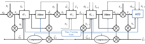
Figure 1: Block diagram of the proposed command filtered backstepping approach.

Remark 4

The filter input involves the virtual controller output, the outputs of the filter and the virtual controller are injected into the compensator dynamics via a subtraction calculation, meanwhile, the outputs of the compensator and the filter are injected into the controller via the “softening” sign function, thereby forming an interconnected closed-loop system. The expressions of (9), (10) and (13) show the specific structure of the filter, compensator and controller, while revealing how to deploy the time-varying feedback signal reasonably. Note that we here do not consider the system in the presence of unmodeled dynamics and parameter uncertainties. The reason for this is that we intend to present a plain scheme that precisely and concisely shows the spirit of the interconnected filter/compensator/controller structural design, instead of exploiting robust scaling to the uncertainties or employing adaptive laws to estimate unknown parameters. This, however, does not mean that the proposed method is not compatible with such robust and/or adaptive schemes.

Proposition 1

The conclusion that the compensated signal $\zeta_{i}$ converges to zero as $t$ tends to infinity holds for any bounded virtual control inputs satisfying $\|{\hat{\alpha}}_{i}-\alpha_{i}\|\leq\tau_{i}$ with $\tau_{i}$ being positive constant.

Proof: Choosing a positive definite function $V_{0}=\sum_{i=1}^{n}\zeta_{i}^{2}/2$ as a Lyapunov function candidate, whose time derivative on $[0,T)$ can be obtained by (10),

$$\dot{V}_{0} =-\sum_{i=1}^{n}\left(k_{i}\mu\zeta_{i}^{2}+\frac{l_{i}\zeta_{i}^{2}}{\sqrt{\zeta_{i}^{2}+\sigma_{i}^{2}}}\right)+\sum_{i=1}^{n-1}g_{i}\zeta_{i}({{\hat{\alpha}}}_{i}-\alpha_{i})$$ (14)

By using Lemma 1, one can obtain

$$\dot{V}_{0} \leq-\sum_{i=1}^{n}\left(k_{i}\mu\zeta_{i}^{2}-l_{i}(\sigma_{i}-|\zeta_{i}|)\right)+\sum_{i=1}^{n-1}g_{i}|\zeta_{i}|\tau_{i}$$ (15)

$$\leq-\sum_{i=1}^{n}\left(k_{i}\mu\zeta_{i}^{2}-l_{i}\sigma_{i}\right)-\sum_{i=1}^{n-1}|\zeta_{i}|(l_{i}-g_{i}\tau_{i})$$

$$\leq-\sum_{i=1}^{n}k_{i}\mu\zeta_{i}^{2}+\sum_{i=1}^{n}l_{i}\sigma_{i}$$

where $l_{i}$ is chosen such as $l_{i}\geq g_{i}\tau_{i}$. From Corollary 1, we have that $\{\zeta_{i}\}_{i=1}^{n}$ will converge to zero as $t\rightarrow+\infty.$ $\hfill\blacksquare$

Now, we are in the position to state the main result.

Theorem 1

Consider system (1) under the coordinate transformation (11) and the compensated tracking errors (12). If we design the command filter, compensator and the controller as in (9), (10) and (13). Then, all closed-loop signals are bounded over the entire time domain, and the tracking error $z_{1}$ converges into a computable residual set $\Omega_{z}$ in prescribed-time $T$ and ultimately decays to zero.

Proof: Step 1: Choose the Lyapunov function candidate as $V_{1}=0.5s_{1}^{2}$, then

$$\dot{V}_{1} =s_{1}\dot{s}_{1}=s_{1}(\dot{z}_{1}-\dot{\zeta}_{1})=s_{1}(\dot{x}_{1}-\dot{x}_{d}-\dot{\zeta}_{1})$$ (16)

$$=s_{1}\left(g_{1}(z_{2}+{{\hat{\alpha}}}_{1})+f_{1}-\dot{x}_{d}-\dot{\zeta}_{1}\right)$$

$$=s_{1}\left(g_{1}\alpha_{1}+g_{1}z_{2}+g_{1}({{\hat{\alpha}}}_{1}-\alpha_{1})+f_{1}-\dot{x}_{d}-\dot{\zeta}_{1}\right).$$

According to Lemma 2 and inserting $\dot{\zeta}_{1}$ and $\alpha_{1}$ as defined in (10) and (13) into (16), yields

$$\dot{V}_{1}= -k_{1}\mu s_{1}^{2}-\frac{s_{1}^{2}}{\sqrt{s_{1}^{2}+\sigma_{1}^{2}}}+g_{1}s_{1}s_{2}$$ (17)

$$\leq -k_{1}\mu s_{1}^{2}-|s_{1}|+\sigma_{1}+g_{1}s_{1}s_{2}$$

$$\leq -k_{1}\mu s_{1}^{2}+\sigma_{1}+g_{1}s_{1}s_{2}.$$

Step k: ($k=2,\cdots,n-1$) Choose the Lyapunov function for the $i$-th subsystem candidate as $V_{k}=\sum_{i=1}^{k-1}V_{i}+0.5s_{k}^{2}$, whose time derivative is

$$\dot{V}_{k}= \sum_{i=1}^{k-1}\dot{V}_{i}+s_{k}\dot{s}_{k}=\sum_{i=1}^{k-1}\dot{V}_{i}+s_{k}(\dot{z}_{k}-\dot{\zeta}_{k})$$ (18)

$$= \sum_{i=1}^{k-1}\dot{V}_{i}-s_{k}\dot{\zeta}_{k}+s_{k}g_{k}\alpha_{k}+$$

$$s_{k}\left(g_{k}z_{k+1}+g_{k}({{\hat{\alpha}}}_{k}-\alpha_{k})+f_{k}-\dot{\beta}_{k}\right).$$

According to the definitions of $\alpha_{k}$ and $\dot{\zeta}_{k}$, we have

$$\dot{V}_{k}= \sum_{i=1}^{k}\left(-k_{i}\mu s_{i}^{2}-\frac{s_{i}^{2}}{\sqrt{s_{i}^{2}+\sigma_{i}^{2}}}\right)+g_{k}s_{k}s_{k+1}.$$ (19)

Step n: Consider the Lyapunov function candidate as $V_{n}=\sum_{i=1}^{n-1}V_{i}+0.5s_{n}^{2}$. Similar to the treatment as shown in (16)-(17), according to the definition of $s_{n}$, we have, for $\forall t\in[0,T)$

$$\dot{V}_{n}=\sum_{i=1}^{n-1}\dot{V}_{i}+s_{n}\dot{s}_{n}= \sum_{i=1}^{n-1}\left(-k_{i}\mu s_{i}^{2}-\frac{s_{i}^{2}}{\sqrt{s_{i}^{2}+\sigma_{i}^{2}}}\right)$$ (20)

$$+g_{n-1}s_{n-1}s_{n}+s_{n}(\dot{z}_{n}-\dot{\zeta}_{n}).$$

It follows from (10), (12) and (13) that

$$s_{n}(\dot{z}_{n}-\dot{\zeta}_{n}) =s_{n}(g_{n}u+f_{n}-\dot{{\hat{\alpha}}}_{n-1}-\dot{\zeta}_{n})$$ (21)

$$=s_{n}\left[\left(-k_{n}\mu z_{n}+\dot{{\hat{\alpha}}}_{n-1}-f_{n}-g_{n-1}z_{n-1}\right.\right.$$

$$\left.\left.~{}~{}-\frac{l_{n}\zeta_{n}}{\sqrt{\zeta_{n}^{2}+\sigma_{n}^{2}}}-\frac{s_{n}}{\sqrt{s_{n}^{2}+\sigma_{n}^{2}}}\right)+f_{n}-\dot{{\hat{\alpha}}}_{n-1}\right.$$

$$\left.~{}~{}+k_{n}\mu\zeta_{n}+g_{n-1}\zeta_{n-1}+\frac{l_{n}\zeta_{n}}{\sqrt{\zeta_{n}^{2}+\sigma_{n}^{2}}}\right]$$

$$=-k_{n}\mu s_{n}^{2}-g_{n-1}s_{n-1}s_{n}-\frac{s_{n}^{2}}{\sqrt{s_{n}^{2}+\sigma_{n}^{2}}}.$$

Substituting (21) into (20) yields

$$\dot{V}_{n}=\sum_{i=1}^{n}\left(-k_{i}\mu s_{i}^{2}-\frac{s_{i}^{2}}{\sqrt{s_{i}^{2}+\sigma_{i}^{2}}}\right)\leq-K_{1}\mu V_{n},$$ (22)

where $K_{1}=2\min\{k_{1},\cdots,k_{n}\}$. In fact, according to Lemma 1, $\dot{V}_{n}$ can also be expressed as, for $t\geq T$

$$\dot{V}_{n} \leq\sum_{i=1}^{n}\left(-k_{i}\bar{\mu}s_{i}^{2}+\sigma_{i}-|s_{i}|\right)\leq-K_{1}\bar{\mu}V_{n}+\Gamma_{2},$$ (23)

where $\Gamma_{2}=\sum_{i=1}^{n}\sigma_{i}$. From (22), (23) and Corollary 1, we have that $V_{n}$, as well as $\{s_{i}\}_{i=1}^{n}$, converge to the set

$$\Omega_{s}=\left\{s_{i}\Big{|}|s_{i}|\leq e^{-K(T+T^{2}/\epsilon)}V_{n}(0)\right\}$$ (24)

as $t\rightarrow T$ and finally converge to zero as $t\rightarrow+\infty.$ In order to figure out the convergence properties of $\zeta_{i}$ at $t=T$, we recalling (15) to get that

$$\dot{V}_{0}\leq-K_{0}V_{0}+\Gamma_{0}$$ (25)

where $K_{0}=2(1+T/\epsilon)\min\{k_{1},\cdots,k_{n}\}$ and $\Gamma_{0}=\sum_{i=1}^{n}l_{i}\sigma_{i}(0)$. Integrating both sides of (25) on $[0,t)$ yields $V_{0}(t)\leq e^{-K_{0}t}V_{0}(0)+\left(1-e^{-K_{0}t}\right){\Gamma_{0}}/{K_{0}}$. It is easy to verify that $V_{0}(t)$ converges to the set

$$\Omega_{\zeta}=e^{-K_{0}T}V_{0}(0)+\left(1-e^{-K_{0}T}\right){\Gamma_{0}}/{K_{0}}$$ (26)

as $t\rightarrow T$. Applying Proposition 1 and recalling the fact $z_{i}=s_{i}+\zeta_{i}$, $z_{i}=x_{i}-{{\hat{\alpha}}}_{i-1}$ for $i=1,\cdots,n$, we know that $\{z_{i}\}_{i=1}^{n}$ converge to the set $\Omega_{z}=\Omega_{\zeta}+\Omega_{s}$ as $t\rightarrow T$. Since we have proven that $\lim_{t\rightarrow+\infty}\zeta_{i}=0$ and $\lim_{t\rightarrow+\infty}s_{i}=0$, therefore $\lim_{t\rightarrow+\infty}z_{i}=0$ can be obtained, establishing the same for the tracking error $z_{1}=x_{1}-x_{d}$. Furthermore, it is not difficult to verify that all closed-loop signals are continuous and bounded over the entire time domain. $\hfill\blacksquare$

Remark 5

It should be mentioned that the proposed scheme has the advantages over DSC and command filtered backstepping method [2]-[15]. First, a time-varying error compensation mechanism is introduced to reduce the errors caused by the filter, which, can guarantee that the error compensation signals are practical prescribed-time stable, reducing the influence of errors timely. Second, different from the UUB or practical finite-time stability achieved in the aforementioned works, the proposed method guarantees that the tracking error converges to a residual set within prescribed-time and ultimately converges to zero, a favorable feature in practice.

IV Simulations

Consider a electromechanical system [11] and rewrite its standard model as the following strict-feedback form:

$$\left\{\begin{array}[]{l}\dot{x}_{1}=x_{2}\\ \dot{x}_{2}=x_{3}-\frac{N}{M}\sin(x_{1})-\frac{B}{M}x_{2}\\ \dot{x}_{3}=u-\frac{K_{m}}{ML}x_{2}-\frac{H}{ML}x_{3}\\ y=x_{1}.\end{array}\right.$$ (27)

For simulation, the initial conditions are chosen as $[x_{1}(0);x_{2}(0);x_{3}(0)]=[0.5;0.5;0.5]$, the system parameters are chosen as $M=0.064,~{}N=3.12,~{}B=0.02,~{}K_{m}=0.9,~{}H=5,~{}L=15$, and the reference signal is chosen as $x_{d}=0.5\sin(t)+0.5\sin(0.5t)$. In addition, we set the control parameters as $[l_{1};l_{2};l_{3}]=[0.1;0.4;20]$, $[k_{1};k_{2};k_{3}]=[8;1;1]$, $\epsilon=0.5$, $\delta_{1}=\delta_{2}=0.01$, $T=2s$, and $\sigma_{1}(t)=\sigma_{2}(t)=\sigma_{3}(t)=5e^{-0.01t}$. Fig. 1 shows that the tracking process under the proposed method, and Fig. 2 shows that the inputs and outputs of the prescribed-time command filter and the control input $u$. Fig. 3 shows the trajectories of the compensator signals $\zeta_{i}$ and $s_{i}$. For comparison, we exploit the controllers proposed in [6] and [11], the trajectories of the tracking error under different controllers are shown in Fig. 4. These results verify the effectiveness of the proposed method and it can be clearly seen that the control performance is improved on the basis of existing methods.

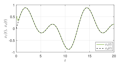
Figure 2: Trajectories of the tracking process.

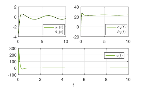
Figure 3: Filter output ${{\hat{\alpha}}}_{1},{{\hat{\alpha}}}_{2}$, virtual control input $\alpha_{1},\alpha_{2}$ and actual control input $u$.

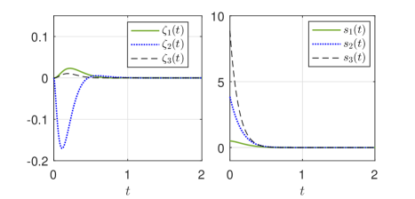
Figure 4: Trajectories of the compensator signals $\{\zeta_{i}(t)\}_{i=1}^{3}$ and the compensated tracking errors $\{s_{i}(t)\}_{i=1}^{3}$.

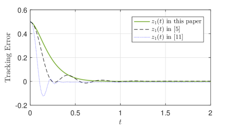
Figure 5: Trajectories of the tracking error $z_{1}$ under different methods.

V Conclusions

In this work we propose a new method of using command filter to simplicity the implementation of the well known backstepping design technique. By using the bounded time-varying scaling, we establish the accelerated filter dynamics, and with proper compensation, we show that the compensator errors converge to zero ultimately and the closed-loop system is asymptotically stable with prescribed performance, opening a new venue for developing backstepping based control algorithms with low-complexity as the issue of “differential explosion” is completely circumvented. Future work includes extending this approach to high-order nonlinear systems with model uncertainties and external disturbances.

References

- [1] M. Krstic, I. Kanelakopoulos, and P. V. Kokotovic, “Adaptive nonlinear control without overparametrization,” Syst. and Control Lett., vol. 19, no. 3, pp. 177-185, Sep. 1992.
- [2] A. Stotsky, J. K. Hedrick, and P. P. Yip, “The use of sliding modes to simplify the backstepping control method,” in Proc. American Contr. Conf., 1997, pp. 1703-1708.
- [3] D. Swaroop, J. K. Hedrick, P. P. Yip, and J. C. Gerdes,“Dynamic Surface Control for a Class of Nonlinear Systems,” IEEE Trans. Automat. Control, vol. 45, no. 10, pp. 1893-1899, Oct. 2000.
- [4] T. P. Zhang, and S. S. Ge, “Adaptive dynamic surface control of nonlinear systems with unknown dead zone in pure feedback form,” Automatica, vol. 44, no. 7, pp. 1859-1903, Jul. 2003.
- [5] Z. R. Zhang, C. Y. Wen, L. T. Xing, and Y. D. Song, “Adaptive Event-Triggered Control of Uncertain Nonlinear Systems Using Intermittent Output Only,” early access, Sep. 2021, doi: 10.1109/TAC.2021.3115435.
- [6] J. A. Farrell, M. Polycarpou, M. Sharma, and W. J. Dong, “Command Filtered Backstepping,” IEEE Trans. Automat. Control, vol. 54, no. 6, pp. 1391-1395, Jun. 2009.
- [7] W. J. Dong, J. A. Farrell, M. M. Polycarpou, V. Djapic, and M. Sharma, “Command Filtered Adaptive Backstepping,” IEEE Trans. Control Syst. Technol., vol. 20, no. 3, pp. 556-580, May. 2012.
- [8] F. Zhang, and G. R. Duan, “Integrated relative position and attitude control of spacecraft in proximity operation missions,” Int. J. Autom. Comput., vol. 9, no. 4, pp. 342-351, Aug. 2012.
- [9] J. L. Du, X. Hu, M. Krstić, and Y. Q. Sun, “Robust dynamic positioning of ships with disturbances under input saturation,” Automatica, vol. 73, pp. 207-214, Nov. 2016.
- [10] K. Zhao, Y. D. Song, and Z. R. Zhang, “Tracking control of MIMO nonlinear systems under full state constraints: A Single-parameter adaptation approach free from feasibility conditions,” Automatica, vol. 107, pp. 52-60. Sep. 2017.
- [11] J. P. Yu, P. Shi, and L. Zhao, “Finite-time command filtered backstepping control for a class of nonlinear systems,” Automatica, vol. 92, pp. 173-180, Jun. 2018.
- [12] Y. J. Wang, and Y. D. Song, “Fraction Dynamic-Surface-Based Neuroadaptive Finite-Time Containment Control of Multiagent Systems in Nonaffine Pure-Feedback Form,” IEEE Trans. Neural Netw. Learn. Syst., vol. 28, no. 3, pp. 678-689, Mar. 2017.
- [13] A. Levant, “Higher-order sliding modes, differentiation and output-feedback control. Int. J. Control, vol. 76, no. 9, pp. 924-941, Oct. 2003.
- [14] J. P. Yu, P. Shi, C. Lin, and H. S. Yu, “Adaptive Neural Command Filtering Control for Nonlinear MIMO Systems With Saturation Input and Unknown Control Direction,” IEEE Trans. Cybern., vol. 50, no. 6, pp. 2536-2545, Jun. 2020.
- [15] L. Zhao, J. P. Yu, and Q. G. Wang, “Finite-Time Tracking Control for Nonlinear Systems via Adaptive Neural Output Feedback and Command Filtered Backstepping,” IEEE Trans. Neural Netw. Learn. Syst., vol. 32, no. 4, pp. 1474-1485, Apr. 2017.
- [16] J. P. Yu, L. Zhao, H. S. Yu, and C. Lin, “Barrier Lyapunov functions-based command filtered output feedback control for full-state constrained nonlinear systems. Automatica, vol. 105, pp. 71-79, Jul. 2019.
- [17] P. Krishnamurthy, F. Khorrami, and M. Krstić, “A dynamic high-gain design for prescribed-time regulation of nonlinear systems,” Automatica, vol. 115, pp. 108860, May. 2020.
- [18] J. S. Huang, W. Wang, C. Y. Wen, and J. Zhou, “Adaptive control of a class of strict-feedback time-varying nonlinear systems with unknown control coefficients,” Automatica, vol. 93, pp. 98-105, Jul. 2018.
- [19] Y. D. Song, Y. J. Wang, J. Holloway, and M. Krstić, “Time-varying feedback for regulation of normal-form nonlinear systems in prescribed finite time,” Automatica, vol. 83, 243-251, Sep. 2017.
- [20] Y. J. Liu, W. Zhao, D. P. Li, S. C. Tong, and C. L. P. Chen, “Adaptive Neural Network Control for a Class of Nonlinear Systems With Function Constraints on States,” IEEE Trans. Neural Netw. Learn. Syst., early access, Sep. 14, 2020, doi: 10.1109/TNNLS.2021.3107600.
- [21] L. Liu, Y. J. Liu, A. Q. Chen, S. C. Tong, and C. L. P. Chen, “Integral Barrier Lyapunov function-based adaptive control for switched nonlinear systems,” Sci. China Inf. Sci., vol. 63, no. 3, pp. 132203, Mar. 2020.
- [22] M. Chen, H. Q. Wang, and X. P. Liu, “Adaptive Practical Fixed-Time Tracking Control With Prescribed Boundary Constraints,” IEEE Trans. Circuits Syst. I, Reg. Papers, vol. 68, no. 4, pp. 1716-1726, Apr. 2021.
- [23] J. Kong, B. Niu, Z. H. Wang, P. Zhao, and W. H. Qi, “Adaptive output-feedback neural tracking control for uncertain switched MIMO nonlinear systems with time delays,” Int. J. Syst. Sci., vol. 52, no. 7, pp. 1-18, Apr. 2021.