A Note on the Construction of Explicit Symplectic Integrators for Schwarzschild Spacetimes

Abstract

In recent publications, the construction of explicit symplectic integrators for Schwarzschild and Kerr type spacetimes is based on splitting and composition methods for numerical integrations of Hamiltonians or time-transformed Hamiltonians associated with these spacetimes. Such splittings are not unique but have various choices. A Hamiltonian describing the motion of charged particles around the Schwarzschild black hole with an external magnetic field can be separated into three, four and five explicitly integrable parts. It is shown through numerical tests of regular and chaotic orbits that the three-part splitting method is the best one of the three Hamiltonian splitting methods in accuracy. In the three-part splitting, optimized fourth-order partitioned Runge-Kutta and Runge-Kutta-Nyström explicit symplectic integrators exhibit the best accuracies. In fact, they are several orders of magnitude better than the fourth-order Yoshida algorithms for appropriate time steps. The former algorithms need small additional computational cost compared with the latter ones. Optimized sixth-order partitioned Runge-Kutta and Runge-Kutta-Nyström explicit symplectic integrators have no dramatic advantages over the optimized fourth-order ones in accuracies during long-term integrations due to roundoff errors. The idea finding the integrators with the best performance is also suitable for Hamiltonians or time-transformed Hamiltonians of other curved spacetimes including the Kerr type spacetimes. When the numbers of explicitly integrable splitting sub-Hamiltonians are as small as possible, such splitting Hamiltonian methods would bring better accuracies. In this case, the optimized fourth-order partitioned Runge-Kutta and Runge-Kutta-Nyström methods are worth recommending.

Unified Astronomy Thesaurus concepts: Black hole physics (159); Computational methods (1965); Computational astronomy (293); Celestial mechanics (211)

1 Introduction

Four basic black hole spacetimes consisting of Schwarzschild, Reissner-Nordström, Kerr and Kerr-Newman metrics are integrable. Although their analytical solutions exist from a theoretical point of view, they cannot be expressed in terms of elementary functions of time and are only formal solutions described by elliptic integrals. Numerical techniques are necessary to study geodesic orbits of particles in these spacetimes. When the spacetimes or their corresponding modified theories of gravity (Deng $\&$ Xie 2016; Deng 2020; Gao $\&$ Deng 2021) contain electromagnetic fields or are immersed in external electromagnetic fields acting as perturbations, they become nonintegrable in many situations. The onset of chaos is even allowed in the nonintegrable systems (Karas $\&$ Vokroulflický 1992; Takahashi $\&$ Koyama 2009; Kopáček $\&$ Karas 2014; Stuchlík $\&$ Kološ 2016; Tursunov et al. 2016; Kopáček $\&$ Karas 2018; Panis et al. 2019; Stuchlík et al. 2020). Numerical techniques are particularly important to solve the nonintegrable problems. Because the spacetimes can exactly correspond to Hamiltonian systems, their most appropriate solvers should maintain the symplectic nature of Hamiltonian dynamics. They are symplectic schemes (Wisdom 1982; Ruth 1983; Feng 1986; Suzuki 1991). They nearly preserve the energy of a conservative mechanical system when truncation errors act as a main error source (see e.g., Hairer et al. 2006). They can also provide reliable results to the integrated trajectories and to the detection of the chaotical behavior for appropriate choices of time steps.

Symplectic methods are divided into explicit symplectic algorithms and implicit ones (Yoshida 1993). Sometimes their compositions (i.e., explicit and implicit symplectic composition methods) are used in the literature (Liao 1997; Preto $\&$ Saha 2009; Lubich et al. 2010; Zhong et al. 2010; Mei et al. 2013a, 2013b). The implicit methods do not need splitting the above-mentioned Hamiltonians, and thus are always available. The implicit midpoint rule (Feng 1986; Brown 2006) and Gauss-Runge-Kutta methods (Kopáček et al. 2010; Seyrich $\&$ Lukes-Gerakopoulos 2012; Seyrich 2013) are common implicit symplectic schemes. They should be generally more expensive in computational cost than the explicit and implicit composition methods at same order. Of course, the latter is more computationally demanding than the explicit algorithms. Many explicit symplectic algorithms usually rely on splitting nonlinear Hamiltonians and composing the flows of the splitting terms. In fact, they are splitting and composition methods for the numerical integration of nonlinear ordinary differential equations. There are a class of explicit symplectic integrators for solving non-separable nonlinear Hamiltonians, which are the product of a function of momenta and another function of coordinates and do not need splittings (Chin 2009). In addition, variational symplectic integrators (Marsden $\&$ West 2001) can be explicit for some nonlinear Hamiltonians without the use of splitting. The implicit midpoint rule as one of the variational symplectic integrators becomes explicit for linear Hamiltonian problems without any splittings.

In general, an $N$-body Hamiltonian problem in the solar system has a classical splitting into two explicitly integrable parts with comparable size, which involve a kinetic energy depending on momenta and a potential energy depending on position coordinates (Ruth 1983). It can also be split into two explicitly integrable terms of different magnitudes, i.e., a primary Kepler part and a small perturbation part corresponding to the interactions among planets (Wisdom $\&$ Holman 1991). This Hamiltonian splitting is a perturbative Hamiltonian splitting method. Explicit symplectic methods, such as fourth-order symplectic integrations of Forest $\&$ Ruth (1990) and higher-order symplectic algorithms of Yoshida (1990), are easily feasible and applicable to the classical splitting and the perturbative splitting. Optimized higher-order partitioned Runge-Kutta (PRK) and Runge-Kutta-Nyström (RKN) explicit symplectic integrators (Blanes $\&$ Moan 2002) are applied for the classical splitting method. However, the pseudo-higher-order symplectic integrators (Chambers $\&$ Murison 2000; Laskar $\&$ Robutel 2001; Blanes et al. 2013) are specifically designed for the perturbative splitting. A splitting of the $N$-body Hamiltonian into three explicitly integrable terms corresponding to various magnitudes was considered by Duncan et al. (1998). The pseudo-higher-order symplectic schemes still work well for such a splitting (Wu et al. 2003). Recently, Chen et al. (2021) split an N-rigid-body Hamiltonian problem into three and four integrable terms with various magnitudes and different timescales. Based on coefficient combinations optimized, the integration accuracy and efficiency are typically improved in the splittings.

The Hamiltonians corresponding to the above-mentioned black-hole spacetimes in general relativity are inseparable to the phase space variables. In spite of this, the above-mentioned explicit symplectic integration algorithms or explicit and implicit combined symplectic methods are always available. When each of the Hamiltonians is split into two terms, not both terms are integrable or have analytical solutions as explicit functions of time. The construction and application of explicit symplectic integrators is difficult for the splitting method. Doubling the phase space variables in any inseparable Hamiltonian problem, Pihajoki (2015) introduced a new Hamiltonian on an extended phase space with two splitting parts equal to the original inseparable Hamiltonian system. Here, one part depends on the original coordinates and the new momenta, and the other part is a function of the original momenta and the new coordinates. The extended phase-space Hamiltonian is amenable for integration with a standard explicit symplectic leapfrog symplectic method. Because both solutions from the leapfrog integrating the two splitting parts are coupled through the derivatives, they should diverge with time. Mixing maps acting as feedback between the two solutions are necessarily included in the leapfrog so as to solve this problem. If the mixing maps are nonsymplectic, then the resulting algorithm no longer symplectic on the extended phase space. Even if the mixing maps are symplectic, the extended phase space leapfrog is not symplectic when a solution in the extended phase space is projected back to that in the original phase space in any case. The best choice of the mixing maps and projection map is that the mixing maps take permutations of momenta, and the projection map takes the original coordinates and the new momenta in the extended phase space as the solution in the original phase space. In this way, the explicit extended phase space algorithm has good long term stability and error behavior although it does not retain the symplecticity, as was numerically confirmed by Pihajoki. Thus, it is a symmetrically symplectic-like method. Liu et al. (2016) pointed out the preference of sequent permutations of coordinates and momenta over the permutations of momenta, and proposed higher order explicit extended phase space symplectic-like integrators for inseparable Hamiltonian systems. Luo et al. (2017) found that the midpoint permutations between the original coordinates and the extended coordinates and the midpoint permutations between the original momenta and the extended momenta are the best mixing maps. The explicit extended phase space symplectic-like integrators with the midpoint permutations are well applicable to nonconservative nonseparable systems (Luo $\&$ Wu 2017), logarithmic Hamiltonians (Li $\&$ Wu 2017), relativistic core-shell spacetimes (Liu et al. 2017), and magnetized Ernst-Schwarzschild spacetimes (Li $\&$ Wu 2019). Recently, Pan et al. (2021) considered the construction of semiexplicit extended phase space symplectic-like integrators for coherent post-Newtonian Euler-Lagrange equations. On the other hand, Tao (2016a) did not adopt any mixing maps and proposed explicit symplectic methods of any even order for a nonseparable Hamiltonian in an extended phase space. In his method, an extended phase space Hamiltonian consists of three parts: two copies of the original system with mixed-up positions and momenta and an artificial restraint with a parameter $\omega$ controlling the binding of the two copies. There are two problems. One problem is that, although the integrators based on the idea of Tao are symplectic in the extended phase space, it is unclear that how the symplecticity of the extended phase space Hamiltonian is related to that of the original system (Jayawardana $\&$ Ohsawa 2021). Another problem is that there is no universal method to find the optimal control parameter $\omega$. The optimal choice relies on only a large number of numerical tests (Wu $\&$ Wu 2018). Combining an extended phase space approach of Pihajoki and a symmetric projection method, Jayawardana $\&$ Ohsawa (2021) have more recently constructed a semiexplicit symplectic integrator for inseparable Hamiltonian systems. The computations of the main time evolution for two copies of the original system with mixed-up positions and momenta are explicit. However, the computations of the symmetric projection that binds potentially diverging copies of solutions are implicit. The resulting method is symplectic in the original phase space.

In fact, it is possible to construct explicit symplectic integrators for the aforementioned curved spacetimes in terms of splitting and composition. One way is a splitting of the Hamiltonians corresponding to these curved spacetimes into more explicitly integrable terms of comparable sizes or different magnitudes. When the Hamiltonian of Schwarzschild spacetime is separated into four integrable splitting parts with analytical solutions as explicit functions of proper time, explicit symplectic methods are easily designed (Wang et al. 2021a). The explicit symplectic methods are also suitable for a splitting of the Hamiltonian of Reissner-Nordström black hole into five explicitly integrable terms (Wang et al. 2021b), and a splitting of the Hamiltonian of Reissner-Nordström-(anti)-de Sitter black hole into six explicitly integrable parts (Wang et al. 2021c). These explicit symplectic methods are still effective when external magnetic fields are included to destroy the integrability of these spacetimes. Unfortunately, no such a similar splitting exists in the Hamiltonian of Kerr black hole and then explicit symplectic methods do not work. Using a time transformation method introduced in the work of Mikkola (1997), Wu et al. (2021) gave a time-transformed Hamiltonian to the Hamiltonian of Kerr black hole. The time-transformed Hamiltonian is separated into five explicitly integrable terms and allows for the application of explicit symplectic methods. This idea was extended to study the chaotic motions of charged particles around the Kerr black holes and deformed Schwarzschild black holes immersed in external magnetic fields (Sun et al. 2021a, 2021b; Zhang et al. 2021). How to choose time transformation functions is dependent on some specific spacetimes. How to split the Hamiltonians or time-transformed Hamiltonians also depends on the specific spacetimes.

Generally, for a splitting of a certain Hamiltonian into many explicitly integrable terms of comparable sizes, the higher-order explicit symplectic methods of Yoshida (1990) are conveniently applied. The optimized fourth- and sixth-order PRK and RKN explicit symplectic integrators (Blanes $\&$ Moan 2002) for the two-part splitting with comparable size can be adjusted as those that are appropriate for the multi-part splitting of comparable sizes (Blanes et al. 2008, 2010). An optimized fourth-order PRK integrator was recently discussed in the splitting method (McLachlan 2021). Compared with the Yoshida constructions, the same order PRK or RKN methods contain more additional time coefficients and more compositions of all sub-Hamiltonian flows. For instance, a fourth-order Yoshida method is a symmetric composition of three second-order leapfrogs, and the optimized fourth-order PRK integrator is that of six pairs of first-order approximation composing all the sub-Hamiltonian flows and the adjoint of the first-order integrator. As a result, the optimized PRK and RKN methods are somewhat more expensive in computations than the same order Yoshida integrators.

Now, there is a question of whether the splitting methods of the above-mentioned or non-mentioned Hamiltonians corresponding to curved spacetimes are unique. If they are not, which of them perform the best accuracies. What performances do the optimized PRK and RKN methods have in various splittings? Are the optimized PRK and RKN methods superior to the same order Yoshida integrators in accuracies? To answer these questions, we consider a Hamiltonian describing the motion of charged particles around the Schwarzschild black hole with an external magnetic field as an example. Besides the splitting of four explicitly integrable parts introduced in the work of Wang et al. (2021a), two splitting methods of three and five explicitly integrable parts with comparable sizes will be given to the Hamiltonian. Then, the fourth- and sixth-order Yoshida algorithms and the fourth- and sixth-order optimized PRK and RKN methods are numerically evaluated in the three splittings. These algorithms combining the explicit extended phase space symplectic methods of Tao (2016a) or the explicit extended phase space symplectic-like integrators with the midpoint permutations of Luo et al. (2017) are numerically compared. In a word, the fundamental aim of the present paper is to find the best integrators and splitting method.

The paper is organized as follows. In Section 2, we introduce three splitting methods to a Hamiltonian system describing the motion of charged particles around the Schwarzschild black hole with an external magnetic field. Yoshida algorithms and optimized PRK and RKN methods of orders 4 and 6 are used in the three splittings. In Section 3, we check the numerical performance of these algorithms in the three splitting methods. Finally, the main results are concluded in Section 4. Some explicit extended phase space symplectic or symplectic-like methods are described in Appendix.

2 Splitting Hamiltonian methods and explicit Symplectic integrators

First, we present a Hamiltonian dynamical system for the description of charged particles moving around the Schwarzschild black hole with an external magnetic field. Second, an existing splitting of the Hamiltonian into four explicitly integrable terms is introduced, and Yoshida algorithms and optimized PRK and RKN methods of orders 4 and 6 are applied to the splitting. Third, a splitting into three explicitly integrable parts is given to the Hamiltonian and these integrators are considered in such a splitting. Finally, the mentioned integrators act on a splitting of the Hamiltonian into five explicitly integrable parts.

2.1 Hamiltonian formulism for Schwarzschild spacetime with external magnetic field

The dynamics of a test particle with charge $q$ moving around the Schwarzschild black hole surrounded by an external magnetic field is described by the following Hamiltonian (Kološ et al. 2015)

$$H=\frac{1}{2}g^{\mu\nu}(p_{\mu}-qA_{\mu})(p_{\nu}-qA_{\nu}).$$ (1)

In spherical-like coordinates $(t,r,\theta,\varphi)$, nonzero components of the Schwarzschild metric $g^{\mu\nu}$ are

$$g^{tt} = -(1-\frac{2}{r})^{-1},~{}~{}~{}~{}~{}~{}g^{rr}=1-\frac{2}{r},$$

$$g^{\theta\theta} = \frac{1}{r^{2}},~{}~{}~{}~{}~{}~{}~{}~{}~{}~{}~{}~{}~{}~{}~{}~{}~{}~{}~{}g^{\varphi\varphi}=\frac{1}{r^{2}\sin^{2}\theta}.$$

The external uniform magnetic field in the vicinity of the black hole has an electromagnetic field potential with only one nonzero covariant component (Kološ et al. 2015; Panis et al. 2019)

$$A_{\varphi}=\frac{B}{2}r^{2}\sin^{2}\theta,$$ (2)

where $B$ represents a magnetic field strength. Here, a point on the presence of magnetic field in the vicinity of the black hole is illustrated. Observations show that strong magnetic fields exist in active galactic nuclei (Xu et al. 2011). A regular magnetic field might arise inside an accretion disk around a black hole due to the dynamo mechanism in conducting matter (plasma) of the accretion disk (Tursunov et al. 2013; Abdujabbarov et al. 2014). This magnetic field does not get through the conducting plasma region and falls in the vicinity of the black hole (Frolov 2012). At large distances, the character of a large-scale magnetic field in accretion processes can be approximately simplified to a homogeneous magnetic field in finite element of space. For simplicity, an asymptotically uniform magnetic field is considered as the external magnetic field (Wald 1974; Kovář et al. 2014; Stuchlík $\&$ Kološ 2016). $p_{\mu}$ is a generalized momentum determined by a set of canonical Hamiltonian equations $\dot{x}^{\mu}=\partial H/\partial p_{\mu}$, and reads

$$p_{\mu}=g_{\mu\nu}\dot{x}^{\nu}+qA_{\mu}.$$ (3)

Here, covariant metric components are $g_{tt}=1/g^{tt}$, $g_{rr}=1/g^{rr}$, $g_{\theta\theta}=1/g^{\theta\theta}$ and $g_{\varphi\varphi}=1/g^{\varphi\varphi}$. 4-velocity $\dot{x}^{\nu}$ is a derivative of coordinate $x^{\nu}$ with respect to proper time $\tau$.

Another set of canonical Hamiltonian equations $\dot{p}_{\mu}=-\partial H/\partial\dot{x}^{\mu}$ show $\dot{p}_{t}=\dot{p}_{\varphi}=0$. Namely, two constant generalized momentum components are

$$p_{t} = g_{tt}\dot{t}=-(1-\frac{2}{r})\dot{t}=-E,$$ (4)

$$p_{\varphi} = g_{\varphi\varphi}\dot{\varphi}+qA_{\varphi}=r^{2}\sin^{2}\theta(\dot{\varphi}+\frac{\beta}{2})=L,$$ (5)

where $\beta=qB$. $E$ is a constant energy of the particle, and $L$ corresponds to a constant angular momentum of the particle. Substituting the two constants into Equation (1), we rewrite the Hamiltonian as

$$H = \frac{1}{2}(1-\frac{2}{r})p_{r}^{2}-\frac{1}{2}(1-\frac{2}{r})^{-1}E^{2}+\frac{p_{\theta}^{2}}{2r^{2}}$$ (6)

$$+\frac{1}{2r^{2}\sin^{2}\theta}(L-\frac{\beta}{2}r^{2}\sin^{2}\theta)^{2}.$$

Due to the particle’s rest mass in the time-like spacetime, a third constant is always given by

$$H=-\frac{1}{2}.$$ (7)

No fourth constant exists when the magnetic field is included in the Schwarzschild spacetime. Thus, the Hamiltonian (6) is a nonintegrable system with two degrees of freedom in a four-dimensional phase space.

A point is illustrated here. The speed of light $c$ and the gravitational constant $G$ are measured in terms of geometric units, $c=G=1$. Equation (6) with Equation (7) is dimensionless. The dimensionless operations to the related qualities are implemented through scale transformations to the qualities. That is, $t\rightarrow tM$, $\tau\rightarrow\tau M$, $r\rightarrow rM$, $B\rightarrow B/M$, $E\rightarrow mE$, $p_{r}\rightarrow mp_{r}$, $L\rightarrow mML$, $p_{\theta}\rightarrow mMp_{\theta}$, $q\rightarrow mq$ and $H\rightarrow m^{2}H$, where $M$ denotes the black hole’s mass and $m$ stands for the particle’s mass.

2.2 An existing splitting method

Separations of the variables in the Hamiltonian (6), including the separation of momenta $p_{r}$ and $p_{\theta}$ from coordinates $r$ and $\theta$ or the separation of variables $r$ and $p_{r}$ from variables $\theta$ and $p_{\theta}$, are impossible. In spite of this fact, the Hamiltonian can still be split into two integrable parts with analytical solutions; e.g., one part is composed of the first, second and fourth terms, and another part is the third term. Unfortunately, not both the parts have explicit analytical solutions. Thus, explicit symplectic integrators are not applicable to the Hamiltonian splitting. However, they are available when the Hamiltonian is separated into four parts with explicit analytical solutions explicitly depending on proper time $\tau$, as was shown by Wang et al. (2021a). In what follows, we briefly introduce the idea on the construction of explicit symplectic methods.

Wang et al. (2021a) suggested splitting the Hamiltonian (6) into four parts as follows:

$$H = H_{1}+H_{2}+H_{3}+H_{4},$$ (8)

$$H_{1} = \frac{1}{2r^{2}\sin^{2}\theta}(L-\frac{\beta}{2}r^{2}\sin^{2}\theta)^{2}$$ (9)

$$-\frac{1}{2}(1-\frac{2}{r})^{-1}E^{2},$$

$$H_{2} = \frac{1}{2}p_{r}^{2},$$ (10)

$$H_{3} = -\frac{1}{r}p_{r}^{2},$$ (11)

$$H_{4} = \frac{1}{2r^{2}}p_{\theta}^{2}.$$ (12)

It is clear that each of the four sub-Hamiltonians $H_{1}$, $H_{2}$, $H_{3}$ and $H_{4}$ is analytically solvable, and its analytical solutions are explicit functions of proper time $\tau$. The exact solvers for the four parts are in sequence labelled as $\Xi_{h}^{H_{1}}$, $\Xi_{h}^{H_{2}}$, $\Xi_{h}^{H_{3}}$ and $\Xi_{h}^{H_{4}}$, where $h$ is a proper time step.

2.2.1 Yoshida’s Constructions

The exact flow of Hamiltonian (6) advancing time $h$, $\Xi_{h}^{H}$, is approximately expressed as

$$\Xi_{h}^{H}\approx S2A(h) = \Xi_{h/2}^{H_{4}}\times\Xi_{h/2}^{H_{3}}\times\Xi_{h/2}^{H_{2}}\times\Xi_{h}^{H_{1}}$$ (13)

$$\times\Xi_{h/2}^{H_{2}}\times\Xi_{h/2}^{H_{3}}\times\Xi_{h/2}^{H_{4}}.$$

S2 is a symmetric composition product of these solvable operators $\Xi_{h}^{H_{1}}$, $\Xi_{h/2}^{H_{2}}$, $\Xi_{h/2}^{H_{3}}$ and $\Xi_{h/2}^{H_{4}}$. It is a second-order explicit symplectic solver for the Hamiltonian (6). Symmetric products of S2A solvers can produce fourth- and sixth-order explicit symplectic schemes (Yoshida 1990):

$$S4A(h)=S2A(c_{1}h)\times S2A(c_{2}h)\times S2A(c_{1}h),$$ (14)

$$S6A=S4A(d_{1}h)\times S4A(d_{2}h)\times S4A(d_{1}h).$$ (15)

where $c_{1}=1/(2-2^{1/3})$, $c_{2}=1-2c_{1}$, $d_{1}=1/(2-2^{1/5})$ and $d_{2}=-2^{1/5}/(2-2^{1/5})$.

These explicit symplectic algorithms proposed by Wang et al. (2021a) are specifically designed for the Schwarzschild type spacetimes without or with perturbations from weak external sources like magnetic fields. The Hamiltonian splitting (8) is also suitable for the construction of higher order optimized explicit symplectic algorithms of Blanes et al. (2010), who introduced symmetric compositions using more extra stages.

2.2.2 Optimized symplectic PRK and RKN methods

Consider two first-order approximations to the exact solutions of the system (8):

$$\chi_{Ah} = \Xi_{h}^{H_{4}}\times\Xi_{h}^{H_{3}}\times\Xi_{h}^{H_{2}}\times\Xi_{h}^{H_{1}},$$ (16)

$$\chi_{Ah}^{*} = \Xi_{h}^{H_{1}}\times\Xi_{h}^{H_{2}}\times\Xi_{h}^{H_{3}}\times\Xi_{h}^{H_{4}}.$$ (17)

Note that $\chi_{Ah}^{*}=\chi_{A(-h)}^{-1}$ is the adjoint of $\chi_{Ah}$. Using both maps $\chi_{Ah}$ and $\chi_{Ah}^{*}$, Blanes et al. (2008, 2010) introduced a symmetric composition

$$\psi_{As}=\chi_{A\alpha_{2s}h}\times\chi^{*}_{A\alpha_{2s-1}h}\times\cdots\times\chi^{*}_{A\alpha_{2}h}\times\chi_{A\alpha_{1}h},$$ (18)

where a series of coefficients are $\alpha_{0}=\alpha_{2s+1}=0$, and

$$\alpha_{1} = a_{1},$$ (19)

$$\alpha_{2j+1} = a_{1}+\sum_{k=1}^{j}(a_{k+1}-b_{k}),$$ (20)

$$\alpha_{2j} = \sum_{k=1}^{j}(b_{k}-a_{k}).$$ (21)

In the above equations, coefficients $a_{1}$, $\cdots$, $b_{1}$, $\cdots$ with $\sum_{i=1}^{s}a_{i}=\sum_{i=1}^{s}b_{i}$ are stemmed from those of the symmetric fourth- and sixth-order symplectic partitioned Runge-Kutta (PRK) and Runge-Kutta-Nyström (RKN) methods for the two-part splitting, and are listed in Tables 2 and 3 by Blanes $\&$ Moan (2002).

When $s=1$, Equation (18) is the second-order algorithm (13):

$$S2A=\chi_{Ah/2}\times\chi^{*}_{Ah/2}.$$ (22)

Such a pair of operator $\chi$ and its adjoint $\chi^{*}$ can compose higher-order integrators.

Given $s=6$, Equation (18) corresponds to a fourth-order optimal explicit symplectic PRK algorithm

$$PRK_{6}4A=\chi_{A\alpha_{12}h}\times\chi^{*}_{A\alpha_{11}h}\cdots\chi^{*}_{A\alpha_{2}h}\times\chi_{A\alpha_{1}h},$$ (23)

where $\alpha_{1}$, $\cdots$, and $\alpha_{12}$ calculated by us are given in Table 1. The optimization means that free coefficients among coefficients $a_{i}$, $b_{i}$ minimize the truncation errors at the fifth order. The free coefficients arise because the number of coefficients $a_{i}$, $b_{i}$ is more than that of the order conditions. The optimization can drastically lead to reducing discretization errors at fixed cost, compared with the non-optimization. McLachlan (2021) confirmed that the ordering of the separable terms in the algorithm affects the errors and slightly affects the computational cost. Thus, choosing the best ordering is important to reduce the errors. Clearly, the optimized fourth-order PRK integrator contain more additional time coefficients and more compositions of all sub-Hamiltonian flows than the fourth-order Yoshida method. In fact, the former is a symmetric composition of six pairs of operator $\chi$ and its adjoint $\chi^{*}$, and the latter is that of three second-order methods S2A.

For $s=10$ in Equation (18), a sixth-order optimal explicit symplectic PRK method is

$$PRK_{10}6A=\chi_{A\alpha_{20}h}\times\chi^{*}_{A\alpha_{19}h}\cdots\chi^{*}_{A\alpha_{2}h}\times\chi_{A\alpha_{1}h},$$ (24)

where the values of $\alpha_{1}$-$\alpha_{20}$ are listed in Table 1. This integrator is a symmetric composition of ten pairs of operator $\chi$ and its adjoint $\chi^{*}$.

On the other hand, Equation (18) can also yield RKN methods. Taking $s=6$, we have a fourth-order optimal explicit symplectic RKN method

$$RKN_{6}4A=\chi_{A\alpha_{12}h}\times\chi^{*}_{A\alpha_{11}h}\cdots\chi^{*}_{A\alpha_{2}h}\times\chi_{A\alpha_{1}h}.$$ (25)

Given $s=11$, a sixth-order optimal explicit symplectic RKN method reads

$$RKN_{11}6A=\chi_{A\alpha_{22}h}\times\chi^{*}_{A\alpha_{21}h}\cdots\chi^{*}_{A\alpha_{2}h}\times\chi_{A\alpha_{1}h}.$$ (26)

For $s=14$, another sixth-order optimal explicit symplectic RKN method is

$$RKN_{14}6A=\chi_{A\alpha_{28}h}\times\chi^{*}_{A\alpha_{27}h}\cdots\chi^{*}_{A\alpha_{2}h}\times\chi_{A\alpha_{1}h}.$$ (27)

We use Equations (19)-(21) to calculate the coefficients of the three algorithms, which are listed in Table 1.

The PRK and RKN methods for the Hamiltonian splitting (8) need more compositions of operators $\Xi_{h}^{H_{1}}$, $\Xi_{h}^{H_{2}}$, $\Xi_{h}^{H_{3}}$ and $\Xi_{h}^{H_{4}}$ than the same order Yoshida’s constructions. Such a splitting Hamiltonian method is not unique. There are other splitting Hamiltonian methods to construct explicit symplectic schemes.

2.3 Other Hamiltonian splitting methods

We focus on the application of the aforementioned integrators to two splittings of the Hamiltonian into three and five explicitly integrable terms.

2.3.1 Splitting three parts

The Hamiltonian (6) can be split into three parts

$$H=H_{1}+\mathcal{H}_{2}+H_{3},$$ (28)

where $\mathcal{H}_{2}$ is the sum of $H_{2}$ and $H_{4}$:

$$\mathcal{H}_{2}=\frac{1}{2}p_{r}^{2}+\frac{1}{2r^{2}}p_{\theta}^{2}.$$ (29)

The canonical equations of sub-Hamiltonian $\mathcal{H}_{2}$ are written as

$$\frac{dr}{d\tau} = \frac{\partial\mathcal{H}_{2}}{\partial p_{r}}=p_{r},~{}~{}\frac{dp_{r}}{d\tau}=-\frac{\partial\mathcal{H}_{2}}{\partial r}=\frac{p^{2}_{\theta}}{r^{3}};$$ (30)

$$\frac{d\theta}{d\tau} = \frac{\partial\mathcal{H}_{2}}{\partial p_{\theta}}=\frac{p_{\theta}}{r^{2}},~{}~{}\frac{dp_{\theta}}{d\tau}=-\frac{\partial\mathcal{H}_{2}}{\partial\theta}=0.$$ (31)

They are exactly, analytically solved. Advancing time $h$ from solutions $(r_{n-1},\theta_{n-1},p_{rn-1},p_{\theta n-1})$ at proper time $\tau_{n-1}$, the analytical solutions at proper time $\tau_{n}=\tau_{n-1}+h$ are expressed as

$$r_{n} = \frac{1}{e_{1}\cos\theta_{n-1}+e_{2}\sin\theta_{n-1}},$$ (32)

$$\theta_{n} = f_{1}+\arctan[(e^{2}_{1}+e^{2}_{2})hp_{\theta_{n-1}}+f_{2}],$$ (33)

$$p_{rn} = p_{\theta_{n-1}}(e_{1}\sin\theta_{n-1}-e_{2}\cos\theta_{n-1});$$ (34)

$$e_{1} = \frac{\cos\theta_{n-1}}{r_{n-1}}+\frac{p_{r_{n-1}}\sin\theta_{n-1}}{p_{\theta_{n-1}}},$$

$$e_{2} = \frac{\sin\theta_{n-1}}{r_{n-1}}+\frac{p_{r_{n-1}}\cos\theta_{n-1}}{p_{\theta_{n-1}}},$$

$$f_{1} = \arctan 2(e_{2},e_{1}),$$

$$f_{2} = \tan(\theta_{n-1}-f_{1}).$$

Equations (13)-(15) are rewritten as

$$S2B(h)=\Xi_{h/2}^{H_{3}}\times\Xi_{h/2}^{\mathcal{H}_{2}}\times\Xi_{h}^{H_{1}}\times\Xi_{h/2}^{\mathcal{H}_{2}}\times\Xi_{h/2}^{H_{3}},$$ (35)

$$S4B(h)=S2B(c_{1}h)\times S2B(c_{2}h)\times S2B(c_{1}h),$$ (36)

$$S6B=S4B(d_{1}h)\times S4B(d_{2}h)\times S4B(d_{1}h).$$ (37)

Their constructions are based on the Hamiltonian three-part splitting (28).

Let us define two first-order maps

$$\chi_{Bh} = \Xi^{H_{3}}_{h}\times\Xi^{\mathcal{H}_{2}}_{h}\times\Xi^{H_{1}}_{h},$$ (38)

$$\chi_{Bh}^{*} = \Xi^{H_{1}}_{h}\times\Xi^{\mathcal{H}_{2}}_{h}\times\Xi^{H_{3}}_{h}.$$ (39)

Through $\chi_{Ah}\rightarrow\chi_{Bh}$ and $\chi^{*}_{Ah}\rightarrow\chi^{*}_{Bh}$, algorithms $PRK_{6}4A$, $PRK_{10}6A$, $RKN_{6}4A$, $RKN_{11}6A$ and $RKN_{14}6A$ become methods $PRK_{6}4B$, $PRK_{10}6B$, $RKN_{6}4B$, $RKN_{11}6B$ and $RKN_{14}6B$, respectively.

2.3.2 Splitting five parts

Now, we give five separable parts to the Hamiltonian (6) as follows:

$$H=H_{1}+\mathbb{H}_{2}+H_{3}+H_{4}+H_{5},$$ (40)

where two new sub-Hamiltonians are

$$\mathbb{H}_{2} = \frac{1}{2}(1+ar)p_{r}^{2},$$ (41)

$$H_{5} = -\frac{ar}{2}p_{r}^{2}.$$ (42)

Here, $a$ is a free parameter. Various choices of $a$ correspond to different five part Hamiltonian decompositions. In other words, there are an infinite number of methods for the Hamiltonian split into five parts.

Sub-Hamiltonian $\mathbb{H}_{2}$ corresponds to evolution equations

$$\frac{dr}{d\tau} = (1+ar)p_{r},$$ (43)

$$\frac{dp_{r}}{d\tau} = -\frac{a}{2}p_{r}^{2}.$$ (44)

The two equations have the analytical solutions

$$r_{n} = \frac{1}{a}[(-\frac{h}{2}ap_{r_{n-1}}(1+ar_{n-1})^{1/2}$$ (45)

$$+(1+ar_{n-1})^{1/2})^{2}-1],$$

$$p_{rn} = (-\frac{ah}{2}+\frac{1}{p_{r_{n-1}}})^{-1}.$$ (46)

For sub-Hamiltonian $H_{5}$, the equations of motion are

$$\frac{dr}{d\tau} = -arp_{r},$$ (47)

$$\frac{dp_{r}}{d\tau} = \frac{a}{2}p_{r}^{2}.$$ (48)

Their analytical solutions read

$$r_{n} = \frac{1}{a}[-\frac{ahp_{r_{n-1}}r^{1/2}_{n-1}}{2}+r^{1/2}_{n-1}]^{1/2},$$ (49)

$$p_{r_{n}} = (-\frac{ah}{2}+\frac{1}{p_{r_{n-1}}})^{-1}.$$ (50)

Equations (13)-(15) become

$$S2C(h) =\Xi_{h/2}^{H_{5}}\times\Xi_{h/2}^{H_{4}}\times\Xi_{h/2}^{H_{3}}\times\Xi_{h/2}^{\mathbb{H}_{2}}\times\Xi_{h}^{H_{1}}$$ (51)

$$\times\Xi_{h/2}^{\mathbb{H}_{2}}\times\Xi_{h/2}^{H_{3}}\times\Xi_{h/2}^{H_{4}}\times\Xi_{h/2}^{H_{5}},$$

$$S4C(h)=S2C(c_{1}h)\times S2C(c_{2}h)\times S2C(c_{1}h),$$ (52)

$$S6C=S4C(d_{1}h)\times S4C(d_{2}h)\times S4C(d_{1}h).$$ (53)

Take two first-order maps

$$\chi_{Ch} = \Xi_{h}^{H_{5}}\times\Xi_{h}^{H_{4}}\times\Xi_{h}^{H_{3}}\times\Xi_{h}^{\mathbb{H}_{2}}\times\Xi_{h}^{H_{1}},$$ (54)

$$\chi^{*}_{Ch} = \Xi_{h}^{H_{1}}\times\Xi_{h}^{\mathbb{H}_{2}}\times\Xi_{h}^{H_{3}}\times\Xi_{h}^{H_{4}}\times\Xi_{h}^{H_{5}}.$$ (55)

In terms of $\chi_{Ah}\rightarrow\chi_{Ch}$ and $\chi^{*}_{Ah}\rightarrow\chi^{*}_{Ch}$, algorithms $PRK_{6}4A$, $PRK_{10}6A$, $RKN_{6}4A$, $RKN_{11}6A$ and $RKN_{14}6A$ correspond to methods $PRK_{6}4C$, $PRK_{10}6C$, $RKN_{6}4C$, $RKN_{11}6C$ and $RKN_{14}6C$, respectively.

Two points are worth noticing. First, the above-mentioned three, four and five splitting parts might have comparable sizes sometimes, or might have various magnitudes and different timescales. In other words, these splitting parts do not always have various magnitudes, and should be considered to be comparable sizes in the whole course of integration. Therefore, the optimized coefficient combinations in the explicit symplectic integrations for the N-rigid-body Hamiltonian problem into three and four integrable terms of various magnitudes and different timescales (Chen et al. 2021) are not suitable for the present splitting and composition methods. Second, if the asymptotically uniform magnetic field in Equation (2) gives place to the general magnetic fields of Tao (2016b), the present splitting and composition methods fail to construct the explicit symplectic methods. However, the Tao’s explicit symplectic integrators are still valid. In fact, the Tao’s construction is unlike ours. In the Tao’s method, one of the two Hamiltonian splitting parts has an analytical solution, whereas another part is not analytically available and uses Runge-Kutta approximation to calculate position. In our construction, each of the Hamiltonian splitting parts is solved analytically.

3 Numerical comparisons

In this section, we mainly check the numerical performance of the above-mentioned algorithms in the three splitting Hamiltonian methods. For comparison, the explicit extended phase space symplectic-like methods with the midpoint permutations of Luo et al. (2017) and the explicit extended phase space symplectic methods without any permutations of Tao (2016a) are considered. Their details are introduced in Appendix.

3.1 Best choice of $a$ in the five splitting parts

The parameters are $E=0.995$, $L=4.6$, and $\beta=8.9\times 10^{-4}$. The initial conditions are $\theta=\pi/2$ and $p_{r}=0$; the initial value $p_{\theta}>0$ is determined by Equation (7). Taking $a=h=1$, we employ the second-order method S2C to plot Figure 1, which describes two orbits with the initial separations $r=11$, 72 in Poincaré surface of section $\theta=\pi/2$ with $p_{\theta}<0$. The initial separation $r=11$ corresponds a closed curve, which indicates regular motion. The motion for the initial separation $r=72$ is chaotic because the plotted points are randomly distributed in an area. The orbital regularity or chaoticity for any conservative Hamiltonian system with two degrees of freedom in four-dimensional phase space can be seen clearly from the distribution of the points in the Poincaré map.

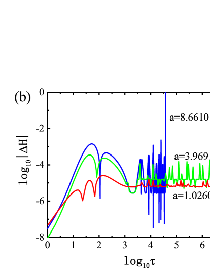
Figure 2: (a) Dependence of Hamiltonian error $\Delta H=1+2H$ for S2C solving the ordered orbit in Figure 1 on $a$. (b) Three values of $a$ in panel (a) correspond to Hamiltonian errors. Clearly, $a=1.0260$ corresponds to the smallest error. It is considered in later computations of the five-part splitting.

Let us choose the regular orbit with the initial separation $r=11$ as a test orbit to evaluate how a variation of $a$ affects the numerical performance of S2C. When $a$ ranges from 0 to 10 with an interval $\Delta a=0.01$, the dependence of Hamiltonian error $\Delta H=1+2H$ on $a$ is shown in Figure 2(a), where each error is obtained by S2C after the integration time $\tau=10^{7}$. Clearly, $a=1.0260$ corresponds to the minimum error. This result is also supported in Figure 2(b) on the description of Hamiltonian errors for $a=1.0260$, 3.9691, 8.6610. Hereafter, $a=1.0260$ is used in the C type algorithms for the Hamiltonian five-part splitting (40).

3.2 Checking numerical performance

Now, the ordered orbit in Figure 1 is still used as a test orbit. The second-order, fourth-order and sixth-order symplectic schemes of Yoshida are applied to the three Hamiltonian splitting methods. The Hamiltonian errors of these algorithms are described in Figures 3 (a)-(c). They remain stable and bounded, and do not grow with time. When truncation errors are larger than roundoff errors, the boundness of Hamiltonian (or energy) errors in long-term integrations is the intrinsic property of these symplectic integrators. Different Hamiltonian splitting methods affect numerical errors. In accuracies, the fourth-order methods are better than the second-order ones, but poorer than the sixth-order ones; at same orders, the B type algorithms are always superior to the A type methods, which are inferior to the C type integrators. Namely, the three-part splitting method has the best accuracy, whereas the five-part splitting method performs the poorest accuracy for a given integrator. When the ordered orbit in Figure 1 is replaced with the chaotic orbit, the results are still the absence of error growth for the second- and fourth-order schemes. The preference of the fourth-order schemes over the second-order schemes, and the preference of the B type algorithms over the A type methods at the second and fourth orders are shown in Figures 3 (d) and (e). However, the errors of the sixth-order method in the three Hamiltonian splittings are almost the same and begin to yield a secular drift when the integration time spans $10^{5}$ in Figure 3(f). This drift is due to roundoff errors. The truncation errors are appropriately accurate to the machine double precision before the integration time $\tau=1000$. As the integration continues, the roundoff errors slowly increase and dominate the truncation errors. This leads to the drift in the errors. Thus, the accuracies of the sixth-order algorithms have no advantage over those of the fourth-order methods when the integration time is long enough. Comparisons between Figures 3(a) and 3(d), comparisons between Figures 3(b) and 3(e), and comparisons between Figures 3(c) and 3(f) show that each of the integrators for the same Hamiltonian splitting exhibits better energy accuracy for the chaotic orbit than for the ordered orbit. This result is due to the average period of the chaotic orbit larger than that of the regular orbit. Although the chaotic orbit lacks periodicity, its average period is admissible. Given a time step, a larger average orbital period should bring better accuracy. On the contrary, the accuracy of solutions becomes poorer for the chaotic case than for the regular case. This is because sensitive dependence of the solutions on the initial conditions for the chaotic case must give rise to the rapid accumulation of errors of the solutions.

What about the numerical performance of the PRK and RKN integrators for the three splitting methods? The ordered orbit in Figure 1 is still chosen as a test orbit. Figures 4 (a) and (b) still support the results described in Figures 3 (a)-(e). That is, the B type algorithms have the best accuracies in the fourth-order optimized methods $PRK_{6}4$ and $RKN_{6}4$, but the C type algorithms yield the poorest accuracies. The B type sixth-order methods in Figures 4 (c) and (d) are better than the A ones within the integration time $\tau=10^{6}$. As the integration time lasts long enough, $PRK_{10}6B$ is inferior to $PRK_{10}6A$, and $RKN_{11}6B$ is inferior to $RKN_{11}6A$ due to the fast growth of roundoff errors. In Figure 4(e), the energy error for $RKN_{14}6B$ is smaller than that for $RKN_{14}6A$, and both errors have no secular drifts. However, the energy error for $RKN_{14}6B$ has one or two orders of magnitude larger than for $RKN_{11}6B$ in Figure 4(d) and $PRK_{10}6B$ in Figure 4(c). Thus, the influence of the roundoff errors on the global errors is smaller for $RKN_{14}6B$ than for $RKN_{11}6B$ and $PRK_{10}6B$. Table 2 lists CPU times of these algorithms solving the regular orbit in Figures 3 and 4. The higher the order of an algorithm is, the more CPU time the algorithm takes. Although CPU time with 3 minutes 23 seconds for $RKN_{14}6C$ is more than CPU time with 32 seconds for S2A, additional CPU time with 2 minutes 51 seconds is still acceptable. In particular, $PRK_{6}4B$ and $RKN_{6}4B$ have appropriately same CPU times, and need small additional computational cost compared with S4B.

The main results of the A and B type algorithms in Figures 3 and 4 are included in Figures 5 (a) and (c). The fourth-order methods from high accuracy to low accuracy in Figure 5(a) are $PRK_{6}4B$ $\succ$ $RKN_{6}4B$ $\succ$ $PRK_{6}4A$ $\succ$ $RKN_{6}4A$ $\succ$ S4B $\succ$ S4A. Note that $PRK_{6}4B$ is slightly better than $RKN_{6}4B$ in accuracy. In particular, the errors of $PRK_{6}4B$ and $RKN_{6}4B$ are four orders of magnitude smaller than that of S4A, and three orders of magnitude smaller than that of S4B. For comparison, the errors of four methods TS4, LS4, TPRK₆4 and LPRK₆4 are plotted in Figure 5(b). TS4 is the Yoshida’s fourth-order construction combining the extended phase space symplectic method of Tao (2016a). LS4 is the Yoshida’s fourth-order construction combining the extended phase space symplectic-like method of Luo et al. (2017). TPRK₆4 is the fourth-order PRK₆4 method combining the Tao’s method. LPRK₆4 is the fourth-order PRK₆4 method combining the method of Luo et al. Their details are given in Appendix. It can be seen clearly from Figures 5 (a) and (b) that TS4 is almost the same as S4A in accuracy. The algorithms from low accuracy to high accuracy are TS4 $\prec$ LS4 $\prec$ S4B $\prec$ TPRK₆4 $\prec$ LPRK₆4 $\prec$ RKN₆4B $\prec$ PRK₆4B. The superiority of the extended phase space symplectic-like methods with the midpoint permutations to the same type extended phase space symplectic methods without the use of any permutations (e.g., LS4 $\succ$ TS4) in accuracy is consistent with that of Wu $\&$ Wu (2018). As far as the CPU times in Table 2 are concerned, the computational efficiency of LS4 is slightly superior to that of TS4. The efficiency of TS4 is close to those of S4A and S4B. The cost of TPRK₆4 is slightly larger than those of RKN₆4B and PRK₆4B, whereas that of LPRK₆4 is slightly smaller. When the integration time is less than $10^{5}$, the sixth-order methods from good accuracy to poor accuracy in Figure 5(c) are $PRK_{10}6B$ $\succ$ $RKN_{11}6B$ $\succ$ $PRK_{10}6A$ $\succ$ $RKN_{11}6A$ $\succ$ $RKN_{14}6B$ $\succ$ S6B $\succ$ $RKN_{14}6A$ $\succ$ S6A. As the integrations continue, the four methods $PRK_{10}6B$, $RKN_{11}6B$, $PRK_{10}6A$ and $RKN_{11}6A$ show secular drifts in the errors. The related errors of these algorithms are clearly listed in Table 3. The fourth-order methods $PRK_{6}4B$ and $RKN_{6}4B$ are four orders of magnitude better in accuracies than the fourth-order Yoshida method S4A or the fourth-order Tao extended phase space method TS4. The sixth-order methods such as $RKN_{11}6B$ have no advantages over the fourth-order methods $PRK_{6}4B$ and $RKN_{6}4B$.

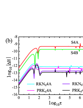
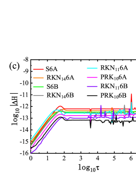
Figure 6: (a) Figure-eight orbit with parameters $E=0.995$, $L=4$, $\beta=1\times 10^{-3}$ and initial separation $r=15.5$ on the Poincaré section. This orbit is described by $PRK_{6}4B$. (b) Hamiltonian errors for all fourth-order A and B type integrators. (c) Hamiltonian errors for all sixth-order A and B type algorithms.

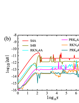
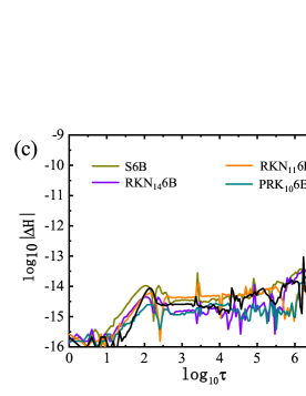
Figure 7: (a) Chaotic orbit with parameters $E=0.992$, $L=4$, $\beta=1.7\times 10^{-3}$ and initial separation $r=25$ on the Poincaré section. This orbit is described by $PRK_{6}4B$. (b) Hamiltonian errors for all fourth-order A and B type integrators. (c) Hamiltonian errors for some sixth-order A and B type algorithms.

Let us investigate the accuracies of the aforementioned algorithms in the three-part and four-part splitting methods for other choices of parameters and initial conditions. Taking $E=0.995$, $L=4$, $\beta=1\times 10^{-3}$ and $r=15.5$, we obtain a figure-eight orbit on the Poincaré section in Figure 6(a). This figure-eight orbit has a hyperbolic fixed point, which corresponds to a stable direction and another unstable direction. It is a separation layer between the regular and chaotic regions. The accuracies of the fourth-order integrators in Figure 6(b) are similar to those in Figure 5(a). There are small differences between Figures 6(b) and 5(a). The accuracy of each integrator in Figure 6(b) is about one order higher than that in Figure 5(a). The accuracies of the sixth-order integrators (such as $PRK_{10}6B$) in Figure 6(c) have no explicit advantages over those of the fourth-order integrators (e.g., $PRK_{6}4B$) in Figure 6(b). When a chaotic orbit with parameters $E=0.992$, $L=4$, $\beta=1.7\times 10^{-3}$ and initial separation $r=25$ in Figure 7(a) is selected as a test orbit, the optimal fourth-order method $PRK_{6}4B$ or $RKN_{6}4B$ in Figure 7(b) has several orders of magnitude better in accuracies than the fourth-order method S4A. The sixth-order methods in Figure 7(c) are not explicitly superior to the fourth-order PRK and RKN methods in Figure 7(b).

The main result can be concluded from Figures 5-7 and Tables 2 and 3. The optimal fourth-order methods $PRK_{6}4B$ and $RKN_{6}4B$ are the best ones of the aforementioned algorithms, and show the best numerical performance in computational accuracy and efficiency.

4 Conclusions

Explicit symplectic integrators are not available for curved spacetimes such as the Schwarzschild or Kerr type spacetimes if the Hamiltonians corresponding to these spacetimes are split into two parts like Hamiltonian problems in the solar system. This is because the two parts lack the separation of variables, are nonintegrable, or have analytical solutions which are not explicit functions of time but are implicit functions of time. A series of recent works (Wang et al. 2021a, 2021b, 2021c; Wu et al. 2021) have successfully worked out this obstacle. The basic idea is splitting the considered Hamiltonians or time-transformed Hamiltonianss into more parts whose analytical solutions are explicit functions of time.

A notable point is that the Hamiltonian splitting method is not unique but has various choices. Taking a Hamiltonian describing the motion of charged particles around the Schwarzschild black hole immersed in an external magnetic field as an example, we can easily separate the Hamiltonian into three, four and five explicitly integrable parts, which are expected to have analytical solutions as explicit functions of time. Errors of an integrator of order 2 or 4 closely depend on the Hamiltonian splitting method. Given an appropriate time step, this integrator shows the best accuracy in the three-part splitting method, but the poorest accuracy in the five-part splitting method. This result is independent of the type of orbits which are regular or chaotic.

It is also found that the optimized fourth-order PRK and RKN explicit symplectic integration schemes in the three-part splitting are several orders of magnitude better in accuracies than the fourth-order Yoshida methods. The former algorithms need small additional computational cost compared with the latter ones. The optimized sixth-order PRK and RKN explicit symplectic integrators have no dramatic advantages over the optimized fourth-order ones in accuracies during long-term integrations due to the rapid accumulation of roundoff errors.

Although the choice of the best explicit symplectic integrators is based on the Schwarzschild spacetime backgrounds, it is applicable to the Kerr type spacetimes or other curved spacetimes. That is, time-transformed Hamiltonians associated with the Kerr type spacetimes, or (time-transformed) Hamiltonians corresponding to the other curved spacetimes, should decrease the number of explicitly integrable splitting parts. Such a splitting method is helpful to decrease the number of computations and then reduces the roundoff errors. In this case, the optimized fourth-order PRK and RKN explicit symplectic integrators will exhibit the best performance.

APPENDIX

Appendix A Extended phase space methods

The four-dimensional phase space Hamiltonian in Equation (6) is labelled as $H=H(r,\theta,p_{r},p_{\theta})$. Following the idea of Pihajoki (2015) and extending the phase space to an eight-dimensional phase space $(r,\theta,\tilde{r},\tilde{\theta},p_{r},p_{\theta},\tilde{p}_{r},\tilde{p}_{\theta})$, we have a new Hamiltonian $\Gamma$ as follows:

$$\Gamma = \Gamma_{1}+\Gamma_{2},$$ (A1)

$$\Gamma_{1} = H(r,\theta,\tilde{p}_{r},\tilde{p}_{\theta}),$$

$$\Gamma_{2} = H(\tilde{r},\tilde{\theta},p_{r},p_{\theta}).$$

Clearly, $\Gamma_{1}$ and $\Gamma_{2}$ are independently analytically solvable. Advancing time $h$, their flows are described by $\Xi^{\Gamma_{1}}_{h}$ and $\Xi^{\Gamma_{2}}_{h}$. Equation (13) becomes

$$S2\Gamma(h)=\Xi^{\Gamma_{1}}_{h/2}\times\Xi^{\Gamma_{2}}_{h}\times\Xi^{\Gamma_{1}}_{h/2}.$$ (A2)

Replacing S2A with S2$\Gamma$ in Equation (14), we obtain a fourth-order explicit symplectic integrator S4$\Gamma$ in the extended phase space. Luo et al. (2017) introduced a midpoint permutation matrix

$$\Psi=\left[\begin{array}[]{cccccccccc}\frac{1}{2}&0&\frac{1}{2}&0&0&0&0&0\\ 0&\frac{1}{2}&0&\frac{1}{2}&0&0&0&0\\ \frac{1}{2}&0&\frac{1}{2}&0&0&0&0&0\\ 0&\frac{1}{2}&0&\frac{1}{2}&0&0&0&0\\ 0&0&0&0&\frac{1}{2}&0&\frac{1}{2}&0\\ 0&0&0&0&0&\frac{1}{2}&0&\frac{1}{2}\\ 0&0&0&0&\frac{1}{2}&0&\frac{1}{2}&0\\ 0&0&0&0&0&\frac{1}{2}&0&\frac{1}{2}\\ \end{array}\right].$$ (A3)

In fact, this matrix means the following transformations

$$r = \tilde{r}\leftarrow\frac{r+\tilde{r}}{2},~{}~{}~{}~{}~{}~{}~{}~{}~{}~{}\theta=\tilde{\theta}\leftarrow\frac{\theta+\tilde{\theta}}{2},$$ (A4)

$$p_{r} = \tilde{p}_{r}\leftarrow\frac{p_{r}+\tilde{p}_{r}}{2},~{}~{}~{}~{}p_{\theta}=\tilde{p}_{\theta}\leftarrow\frac{p_{\theta}+\tilde{p}_{\theta}}{2}.$$ (A5)

The method S4$\Gamma$ combining the matrix $\Psi$ corresponds to a fourth-order explicit scheme

$$LS4=\Psi\times S4\Gamma.$$ (A6)

Due to the inclusion of the permutation $\Psi$, LS4 is a symplectic-like method for the extended phase space Hamiltonian $\Gamma$. Similarly, Equations (16) and (17) become

$$\chi_{\Gamma h}=\Xi_{h}^{\Gamma_{2}}\times\Xi_{h}^{\Gamma_{1}},~{}~{}~{}~{}\chi_{\Gamma h}^{*}=\Xi_{h}^{\Gamma_{1}}\times\Xi_{h}^{\Gamma_{2}}.$$ (A7)

Using $\chi_{\Gamma}$ and $\chi_{\Gamma}^{*}$ instead of $\chi_{A}$ and $\chi_{A}^{*}$ in Equation (23), we have $PRK_{6}4\Gamma$. Thus, an extended phase space PRK explicit symplectic-like method is

$$LPRK_{6}4=\Psi\times PRK_{6}4\Gamma.$$ (A8)

Adding a third part

$$\Gamma_{3}=\frac{\omega}{2}[(r-\tilde{r})^{2}+(\theta-\tilde{\theta})^{2}+(p_{r}-\tilde{p}_{r})^{2}+(p_{\theta}-\tilde{p}_{\theta})^{2}]$$ (A9)

to Equation (A1), Tao (2016a) obtained another new Hamiltonian

$$K=\Gamma+\Gamma_{3}.$$ (A10)

Here, $\omega$ is a parameter controlling the binding of the two copies. Noting that $H_{1}\rightarrow\Gamma_{1}$, $\mathcal{H}_{2}\rightarrow\Gamma_{2}$ and $H_{3}\rightarrow\Gamma_{3}$ in Equation (28), we have TS4 corresponding to S4B in Equation (36) and TPRK₆4 corresponding to PRK₆4B. TS4 and TPRK₆4 are two fourth-order extended phase space explicit symplectic methods for the Hamiltonian $K$. Numerical accuracies depend on the control parameter $\omega$. For $\omega=3.553$ in Figure 8(a), the method TS4 has the best accuracy. For $\omega=7.943$ in Figure 8(b), the method TPRK₆4 performs the best accuracy. The two values of $\omega$ are considered in other computations.

Table 1: Coefficients of optimal explicit symplectic PRK and RKN methods

$PRK_{6}4$: order 4,    $s=6$
$\alpha_{1}=\alpha_{12}=0.079203696431196$	$\alpha_{2}=\alpha_{11}=0.130311410182166$	$\alpha_{3}=\alpha_{10}=0.222861495867608$
$\alpha_{4}=\alpha_{9}=-0.366713268047426$	$\alpha_{5}=\alpha_{8}=0.324648188689706$	$\alpha_{6}=\alpha_{7}=0.109688477876750$
$RKN_{6}4$: order 4,    $s=6$
$\alpha_{1}=\alpha_{12}=0.082984402775764$	$\alpha_{2}=\alpha_{11}=0.162314549088478$	$\alpha_{3}=\alpha_{10}=0.233995243906975$
$\alpha_{4}=\alpha_{9}=0.370877400040627$	$\alpha_{5}=\alpha_{8}=-0.409933704882860$	$\alpha_{6}=\alpha_{7}=0.059762109071016$
$PRK_{10}6$: order 6,    $s=10$
$\alpha_{1}=\alpha_{20}=0.050262764400392$	$\alpha_{2}=\alpha_{19}=0.098553687334061$	$\alpha_{3}=\alpha_{18}=0.314960598945618$
$\alpha_{4}=\alpha_{17}=-0.447346463799477$	$\alpha_{5}=\alpha_{16}=0.492426354438066$	$\alpha_{6}=\alpha_{15}=-0.425118748098612$
$\alpha_{7}=\alpha_{14}=0.237063888460398$	$\alpha_{8}=\alpha_{13}=0.195602502673864$	$\alpha_{9}=\alpha_{12}=0.346358153969049$
$\alpha_{10}=\alpha_{11}=-0.362762738019228$
$RKN_{11}6$: order 6,    $s=11$
$\alpha_{1}=\alpha_{22}=0.041464999318123$	$\alpha_{2}=\alpha_{21}=0.081764779984951$	$\alpha_{3}=\alpha_{20}=0.116363890469074$
$\alpha_{4}=\alpha_{19}=0.174189917743206$	$\alpha_{5}=\alpha_{18}=-0.214196108281612$	$\alpha_{6}=\alpha_{17}=0.087146900594235$
$\alpha_{7}=\alpha_{16}=-0.011892914772034$	$\alpha_{8}=\alpha_{15}=-0.234438851475716$	$\alpha_{9}=\alpha_{14}=0.222927464172244$
$\alpha_{10}=\alpha_{13}=0.134281413629651$	$\alpha_{11}=\alpha_{12}=0.102388508617878$
$RKN_{14}6$: order 6,    $s=14$
$\alpha_{1}=\alpha_{28}=0.037859320640564$	$\alpha_{2}=\alpha_{27}=0.053859829902649$	$\alpha_{3}=\alpha_{26}=0.048775799572468$
$\alpha_{4}=\alpha_{25}=0.135207377374172$	$\alpha_{5}=\alpha_{24}=-0.161075266078115$	$\alpha_{6}=\alpha_{23}=0.104540901258588$
$\alpha_{7}=\alpha_{22}=0.209700508043170$	$\alpha_{8}=\alpha_{21}=-0.204785819165409$	$\alpha_{9}=\alpha_{20}=0.074641357176006$
$\alpha_{10}=\alpha_{19}=0.069119771011173$	$\alpha_{11}=\alpha_{18}=0.037297929637134$	$\alpha_{12}=\alpha_{17}=0.291269754059613$
$\alpha_{13}=\alpha_{16}=-0.3000639975070951$	$\alpha_{14}=\alpha_{15}=0.103652534075081$

Table 2: CPU times (unit: minute^′ second^′′ ) for all integrators acting on the three splitting methods considered in Figures 3, 4 and 5. The test orbit is the regular orbit in Figure 1, and the integration time of each algorithm reaches $\tau=10^{7}$.

Algorithm	S2A	S2B	S2C	S4A	S4B	S4C
CPU Time	0′32′′	1′13′′	1′36′′	1′03′′	1′22′′	1′47′′
Algorithm	S6A	S6B	S6C	$PRK_{6}4A$	$PRK_{6}4B$	$PRK_{6}4C$
CPU Time	2′17′′	2′18′′	2′31′′	1′48′′	1′53′′	2′11′′
Algorithm	$RKN_{6}4A$	$RKN_{6}4B$	$RKN_{6}4C$	$PRK_{10}6A$	$PRK_{10}6B$	$PRK_{10}6C$
CPU Time	2′0′′	2′12′′	2′31′′	2′29′′	2′37′′	2′57′′
Algorithm	$RKN_{11}6A$	$RKN_{11}6B$	$RKN_{11}6C$	$RKN_{14}6A$	$RKN_{14}6B$	$RKN_{14}6C$
CPU Time	2′35′′	2′43′′	3′13′′	2′47′′	2′5′′	3′23′′
Algorithm	$TS4$	$LS4$	$TPRK_{6}4$	$LPRK_{6}4$
CPU Time	1′12′′	0′41′′	2′27′′	1′55′′

Table 3: The minimum and maximum energy errors for all integrators in Figure 5.

Algorithm	Minimum	Maximum	Algorithm	Minimum	Maximum
S4A	$10^{-10.86}$	$10^{-8.09}$	S4B	$10^{-11.56}$	$10^{-8.79}$
S6A	$10^{-13.02}$	$10^{-10.61}$	S6B	$10^{-13.67}$	$10^{-11.52}$
$PRK_{6}4A$	$10^{-13.64}$	$10^{-10.79}$	$PRK_{6}4B$	$10^{-14.78}$	$10^{-12.12}$
$RKN_{6}4A$	$10^{-12.50}$	$10^{-10.55}$	$RKN_{6}4B$	$10^{-13.83}$	$10^{-11.88}$
$PRK_{10}6A$	$10^{-15.15}$	$10^{-12.28}$	$PRK_{10}6B$	$10^{-15.55}$	$10^{-12.06}$
$RKN_{11}6A$	$10^{-13.81}$	$10^{-12.32}$	$RKN_{11}6B$	$10^{-14.81}$	$10^{-12.08}$
$RKN_{14}6A$	$10^{-13.01}$	$10^{-11.22}$	$RKN_{14}6B$	$10^{-13.69}$	$10^{-11.79}$
$TS4$	$10^{-10.98}$	$10^{-8.04}$	$LS4$	$10^{-10.67}$	$10^{-8.54}$
$TPRK_{6}4$	$10^{-12.93}$	$10^{-10.51}$	$LPRK_{6}4$	$10^{-13.36}$	$10^{-10.96}$

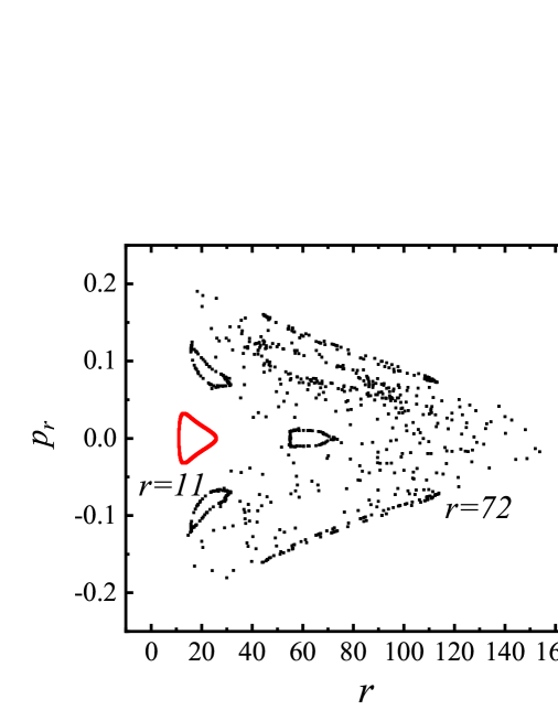
Figure 1: Poincaré surface of section $\theta=\pi/2$ with $p_{\theta}<0$. The time step uses $h=1$, and the parameters are $E=0.995$, $L=4.6$, and $\beta=8.9\times 10^{-4}$. The initial conditions are $\theta=\pi/2$ and $p_{r}=0$; the initial value $p_{\theta}>0$ is determined by Equation (7). The second-order method is applied to the five-part splitting with $a=1$, i.e., S2C. A regular orbit with initial separation $r=11$ colored Red and another chaotic orbit with initial separation $r=72$ colored Black are plotted.

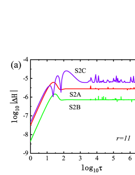
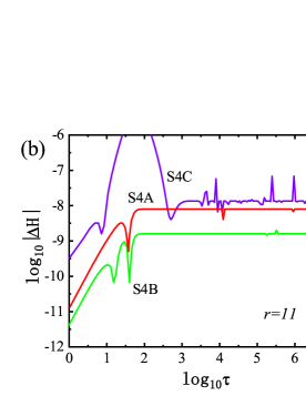
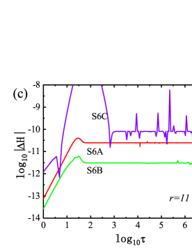
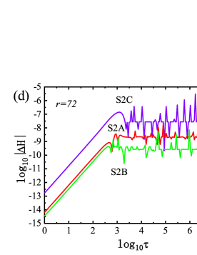
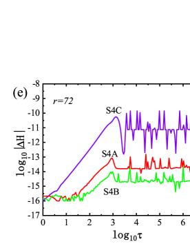
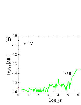
Figure 3: (a-c): Hamiltonian errors for the Yoshida type integrators acting on the regular orbit in Figure 1. (d-f): Similar to panels (a-c) but the regular orbit is replaced with the chaotic orbit in Figure 1. S6A and S6C are almost consistent with S6B.

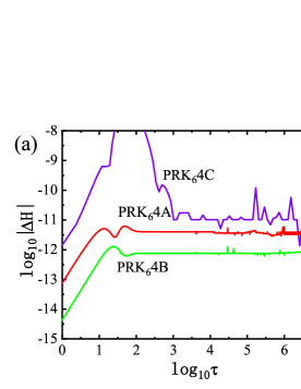
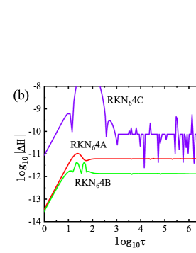
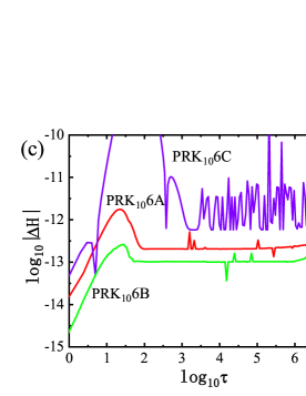
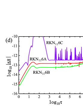
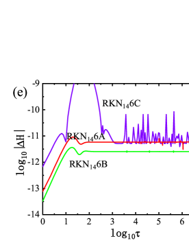
Figure 4: Similar to Figures 3 (a-c) but the PRK and RKN integrators are used in the three Hamiltonian splittings. (a) Optimal fourth-order PRK methods. (b) Optimal fourth-order RKN methods. (c) Optimal sixth-order PRK methods. (d) An optimal sixth-order RKN method. (e) Another optimal sixth-order RKN method.

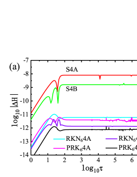
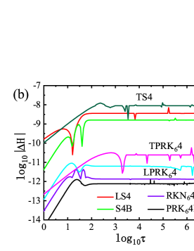
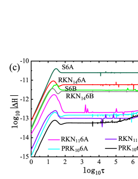
Figure 5: Results concluded from those of the A and B type methods in Figures 3 (a)-(e) and 4. (a) Errors of all fourth-order integrators. (b) Errors of four methods TS4, LS4, TPRK₆4 and LPRK₆4 in Appendix.

(c) Errors of all sixth-order algorithms.

Figure 8: Dependence of Hamiltonian error $\Delta H$ on the control parameter $\omega$. The test orbit is that of Figure 2(a). Let $\omega$ range from 0 to 20 with an interval $\Delta\omega=0.001$. Given a value of $\omega$, the error is obtained after $10^{7}$ integration steps. $\omega=3.553$ corresponds to the best accuracy for TS4 in panel (a), and $\omega=7.943$ does for TPRK₆4 in panel (b).

References

- a (1) Abdujabbarov, A., Ahmedov, B., Rahimov, O., Salikhbaev, U. 2014, Phys. Scr., 89, 084008
- a (1) Blanes, S., Casas, F., Farres, A., Laskar, J., Makazaga, J., Murua, A. 2013, Applied Numerical Mathematics, 68, 58
- a (1) Blanes, S., Casas, F., Murua, A. 2008, Bol. Soc. Esp. Math. Apl., 45, 87
- a (1) Blanes, S., Casas, F., Murua, A. 2010, Bol. Soc. Esp. Math. Apl., 50, 47
- a (1) Blanes, S., Moan, P. C. 2002, Journal of Computational and Applied Mathematics, 142, 313
- a (1) Brown, J. D. 2006, Phys. Rev. D, 73, 024001
- a (1) Chambers, J. E., Murison, M. A. 2000, AJ, 119, 425
- a (1) Chen, R., Li, G., Tao, M. 2021, ApJ, 919, 50
- a (1) Chin, S. A. 2009, Phys. Rev. E, 80, 037701
- a (1) Deng, X.-M. 2020, Eur. Phys. J. C, 80, 489
- a (1) Deng, X.-M, Xie, Y. 2016, Phys. Rev. D, 93, 044013
- a (1) Duncan, M.J., Levision, H .F., Lee, M. H. 1998, AJ, 116, 2067
- a (1) Feng, K. 1986, Journal of Computational Mathematics, 44, 279
- a (1) Forest, E., Ruth, R. D. 1990, Physica D, 43, 105
- a (1) Frolov, V. P. 2012, Phys. Rev. D, 85, 024020
- a (1) Gao, B., Deng, X.-M. 2021, Eur. Phys. J. C, 81, 983
- a (1) Hairer, E., Lubich, C., Wanner, G. 2006, Geometric Numerical Integration: Structure-Preserving Algorithms for Ordinary Differential Equations, second ed. (Springer, Berlin/Heidelberg/New York)
- a (1) Jayawardana, B., Ohsawa, T. 2021, arXiv: 2111. 10915 [Math. Na]
- Karas Vokrouhlický (1992) Karas, V., Vokrouhlický, D. 1992, Gen. Relativ. Gravit., 24, 729
- a (1) Kološ, M., Stuchlík, Z., Tursunov, A. 2015, Class. Quantum Grav., 32, 165009
- a (1) Kopáček, O., Karas, V. 2014, ApJ, 787, 117
- Kopáček & Karas (2018) Kopáček, O., Karas, V. 2018, ApJ, 853, 53
- a (1) Kopáček, O., Karas, V., Kovář, J., Stuchlík, Z. 2010, ApJ, 722, 1240
- a (1) Kovář, J., Slany, P., Cremaschini, C., Stuchlík, Z., Karas, V., Trova, A. 2014, Phys. Rev. D, 90, 044029
- a (1) Laskar, J., Robutel, P. 2001, Celestial Mechanics and Dynamical Astronomy, 80, 39
- a (1) Li, D., Wu, X. 2017, Mon. Not. R. Astron. Soc., 469, 3031
- a (1) Li, D., Wu, X. 2019, Eur. Phys. J. Plus, 134, 96
- a (1) Liao, X. H. 1997, Celest. Mech. Dyn. Astron., 66, 243
- a (1) Liu, L., Wu, X., Huang, G. 2017, Gen. Relativ. Gravit., 49, 28
- a (1) Liu, L., Wu, X., Huang, G., Liu, F. 2016, Mon. Not. R. Astron. Soc., 459, 1968
- a (1) Lubich, C., Walther, B., Brügmann, B. 2010, Phys. Rev. D, 81, 104025
- a (1) Luo, J., Wu, X. 2017, Eur. Phys. J. Plus, 132, 485
- a (1) Luo, J., Wu, X., Huang, G., Liu, F. 2017, ApJ, 834, 64
- a (1) Marsden, J. E., West, M. 2001, Acta Numerica, 10, 357
- a (1) McLachlan, R. I. 2021, arXiv: 2014. 10269 [physics. comp-ph]
- a (1) Mei, L., Ju, M., Wu, X., Liu, S. 2013a, Mon. Not. R. Astron. Soc., 435, 2246
- a (1) Mei, L., Wu, X., Liu, F. 2013b, Eur. Phys. J. C, 73, 2413
- a (1) Mikkola, S. 1997, Celest. Mech. Dyn. Ast., 67, 145
- a (1) Pan, G., Wu, X., Liang, E. 2021, Phys. Rev. D, 104, 044055
- Panis et al. (2019) Panis, R., kolos̆, M., Stuchlík, Z. 2019, Eur. Phys. C, 79, 479
- Pihajoki (2015) Pihajoki, P. 2015, Celest. Mech. Dyn. Astron., 121, 211
- a (1) Preto, M., Saha, P. 2009, ApJ, 703, 1743
- a (1) Ruth, R. D. 1983, IEEE Trans. Nucl. Sci. NS, 30, 2669
- Seyrich (2013) Seyrich, J. 2013, Phys. Rev. D, 87, 084064
- a (1) Seyrich, J., Lukes-Gerakopoulos, G. 2012, Phys. Rev. D, 86, 124013
- Sun et al. (2021) Sun, W., Wang, Y., Liu, F. Y., Wu, X. 2021a, Eur. Phys. J. C, 81, 785.
- a (1) Sun, X., Wu, X., Wang, Y., Deng, C., Liu, B., Liang, E. 2021b, Universe, 7, 410
- a (1) Suzuki, M. 1991, J. Math. Phys. (N.Y.), 32, 400
- Stuchlík Kološ (2016) Stuchlík, Z., Kološ, M. 2016, Eur. Phys. J. C, 76, 32
- a (1) Stuchlík, Z., Kološ, M., Kovář, J., Tursunov, A. 2020, Universe, 6, 26
- a (1) Tao, M. 2016a, Phys. Rev. E, 94, 043303
- a (1) Tao, M. 2016b, Journal of Computational Physics, 327, 245
- a (1) Takahashi, M., Koyama, H. 2009, ApJ, 693, 472
- a (1) Tursunov, A., Kološ, M., Ahmedov, B., Stuchlík, Z. 2013, Phys. Rev. D, 87, 125003
- Tursunov et al. (2016) Tursunov, A., Stuchlík. Z., Kološ, M. 2016, Phys. Rev. D, 93, 084012
- a (1) Wald, R. M. 1974, Phys. Rev. D, 10, 1680
- a (1) Wang, Y., Sun, W., Liu, F., Wu, X. 2021a, ApJ, 907, 66
- a (1) Wang, Y., Sun, W., Liu, F., Wu, X., 2021b, ApJ, 909, 22
- a (1) Wang, Y., Sun, W., Liu, F., Wu, X., 2021c, ApJS, 254, 8
- a (1) Wisdom, J. 1982, AJ, 87, 577
- a (1) Wisdom, J., Holman, M. 1991, AJ, 102, 1528
- Wu et al. (2003) Wu X., Huang T.-Y., Wan X.-S. 2003, Chin. Astron. Astrophys., 27, 114
- Wu et al. (2021) Wu, X., Wang, Y., Sun, W., Liu, F. Y. 2021, ApJ, 914, 63.
- a (1) Wu, Y., Wu, X. 2018, International Journal of Modern Physics C, 29, 1850006
- a (1) Xu, H., Li, H., Collins, D. C., Li, S, Norman, M. L. 2011, ApJ, 739, 77
- a (1) Yoshida, H. 1990, Phys. Lett. A, 150, 262
- a (1) Yoshida, H. 1993, Celest. Mech. Dyn. Astron., 56, 27
- a (1) Zhang, H., Zhou, N., Liu, W., Wu, X. 2021, Universe, submitted
- a (1) Zhong, S. Y., Wu, X., Liu, S. Q., Deng, X. F. 2010, Phys. Rev. D, 82, 124040