A FEAST SVDsolver based on Chebyshev–Jackson series for computing partial singular triplets of large matrices

Abstract

The FEAST eigensolver is extended to the computation of the singular triplets of a large matrix $A$ with the singular values in a given interval. The resulting FEAST SVDsolver is subspace iteration applied to an approximate spectral projector of $A^{T}A$ corresponding to the desired singular values in a given interval, and constructs approximate left and right singular subspaces corresponding to the desired singular values, onto which $A$ is projected to obtain Ritz approximations. Differently from a commonly used contour integral-based FEAST solver, we propose a robust alternative that constructs approximate spectral projectors by using the Chebyshev–Jackson polynomial series, which are symmetric positive semi-definite with the eigenvalues in $[0,1]$. We prove the pointwise convergence of this series and give compact estimates for pointwise errors of it and the step function that corresponds to the exact spectral projector. We present error bounds for the approximate spectral projector and reliable estimates for the number of desired singular triplets, establish numerous convergence results on the resulting FEAST SVDsolver, and propose practical selection strategies for determining the series degree and for reliably determining the subspace dimension. The solver and results on it are directly applicable or adaptable to the real symmetric and complex Hermitian eigenvalue problem. Numerical experiments illustrate that our FEAST SVDsolver is at least competitive with and is much more efficient than the contour integral-based FEAST SVDsolver when the desired singular values are extreme and interior ones, respectively, and it is also more robust than the latter.

1 Introduction

Matrix singular value decomposition (SVD) problems play a crucial role in many applications. For small to moderate problems, very efficient and robust SVD algorithms and softwares have been well developed and widely used golub2013matrix ; stewart2001matrix . They are often called direct SVD solvers, and compute the entire singular values and/or singular vectors using predictable iterations. In this paper, we consider the following partial SVD problem: Given a matrix $A\in\mathbb{R}^{m\times n}$ with $m\geq n\gg 1$ and a real interval $[a,b]$ contained in the singular spectrum of $A$, determine the $n_{sv}$ singular triplets $(\sigma,u,v)$ with the singular values $\sigma\in[a,b]$ counting multiplicities, where

$$\begin{cases}Av=\sigma u,\\ A^{T}u=\sigma v,\\ \left\|u\right\|=\left\|v\right\|=1.\end{cases}$$

Since the SVD of $A$ is mathematically equivalent to the eigendecomposition of its cross-product matrix $A^{T}A$, it is possible to adapt those algorithms for a symmetric matrix eigenvalue problem to the corresponding SVD problem in some numerically stable way. Over the past two decades, a new class of numerical methods has emerged for computing the eigenvalues of a large matrix in a given region and/or the associated eigenvectors, and they are based on contour integration and rational filtering. Among them, representatives are the Sakurai–Sugiura (SS) method sakurai2003projection and the FEAST eigensolver polizzi2009density , which fall into the category of Rayleigh–Ritz projection methods. We should point out that, for the computation of eigenvalues in a given region inside the spectrum, all the other available algorithms, e.g., subspace iteration, Arnoldi type algorithms and their shift-invert variants, and Jacobi–Davidson type algorithms, are not directly applicable. The only exception is that the given region and exterior eigenvalues coincide and the number of eigenvalues in the region is known. In this case, the implicitly restarted Arnoldi algorithm sorensen1992 , on which the package ARPACK lehoucq1998 and the Matlab function eigs are based, and the implicitly restarted refined Arnoldi algorithm jia1999 can be used.

The SS method and subsequent variants ikegami2010contour ; ikegami2010filter ; imakura2014SSarnoldi ; sakurai2016 ; sakurai2007cirr have resulted in the z-Pares package Futamura2014Online that handles large Hermitian and non-Hermitian matrix eigenvalue problems. The original SS method is the SS-Hankel method, and its variants include the SS-RR method (Rayleigh–Ritz projection) and the SS-Arnoldi method as well as their block variants. The SS-Hankel method computes certain moments, which are constructed by the contour integrals with an integral domain containing all the desired eigenvalues, to form small Hankel matrices or matrix pairs of order $m$, whose eigenvalues equal the desired $m$ distinct eigenvalues of the original matrix or matrix pair contained in the region. In computations, one computes those contour integrals by some numerical quadrature and obtains approximations to the moments, or constructs an approximate spectral projector associated with all the desired eigenvalues if the exact spectral projector is involved. The SS method and its variants are essentially Krylov or block Krylov subspace based methods starting with a specific initial vector or block vector that is generated by acting the approximate spectral projector on a vector or block vector chosen randomly, realize the Rayleigh–Ritz projection onto them, and compute Ritz approximations sakurai2016 . The SS-RR method computes an orthonormal basis of the underlying subspace and projects the large matrix or matrix pair onto it, and the SS-Arnoldi method exploits the Arnoldi process to generate an orthonormal basis of the subspace and forms the projection matrix. We refer the reader to sakurai2016 for a summary of these methods.

The FEAST eigensolver guttel2015zolotarev ; kestyn2016feast ; polizzi2009density ; tang2014feast , first introduced by Polizzi polizzi2009density in 2009, has led to the development of the FEAST numerical library polizzi2020feast . Unlike the SS method and its variants, this eigensolver works on subspaces of a fixed dimension and uses subspace iteration golub2013matrix ; parlett1998symmetric ; saad2011numerical ; stewart2001matrix on an approximate spectral projector to generate a sequence of subspaces, onto which the Rayleigh–Ritz projection of the original matrix or matrix pair is realized and the Ritz approximations are computed.

In the SS-method and the FEAST eigensolver, since the spectral projector associated with the eigenvalues in a given region can be represented in the form of a contour integral, computationally they use a suitably chosen quadrature to approximate the integral and construct an approximate spectral projector. This involves solutions of several linear systems with shifted coefficient matrices, where the shifts are the quadrature nodes. For instance, the FEAST eigensolver needs to solve several, i.e., the subspace dimension times the number of nodes, large linear systems at each iteration. If the matrix is structured, such as banded, then one can use LU factorizations golub2013matrix to solve the linear systems involved efficiently. But if the matrix is generally dense or sparse, ones needs to apply some iterative methods, e.g., Krylov subspace iterative methods, to solve them approximately, and the resulting algorithm is called IFEAST gavin2018ifeast . However, these linear systems are highly indefinite when the region of interest is inside the spectrum. It is well known that, for highly indefinite or nonsymmetric linear systems, Krylov subspace iterative solvers, e.g., the GMRES and BiCGstab methods saad2003 , are generally inefficient and can be very slow. An adaptation of Theorem 3.1 of robbe2009 on inverse subspace iteration to the current context states that these shifted linear systems must be solved with increasing accuracy in order to guarantee that the FEAST eigensolver converges linearly gavin2018ifeast . As a consequence, the FEAST eigensolver may be extremely slow even if these linear systems are solved in parallel. We should point out that there has not yet been a general effective preconditioning technique for highly indefinite linear systems.

As a matter of fact, the situation is more subtle. It is known from tang2014feast that the distance between a desired eigenvector and the subspace may only decrease down to the relative accuracy level of the approximate solutions of the shifted linear systems rather than the residual norm level. This implies that, in finite precision, the residual norm of an approximate eigenpair by the FEAST solver may not drop below a reasonably prescribed tolerance, say $10^{-13}$, once one of the shifted linear systems is ill conditioned, which is definitely true when some of the nodes are close to some eigenvalues of the underlying matrix.

More precisely, it is well known that the attainable relative error, i.e., the relative accuracy, of an approximate solution is bounded by the condition number times by the relative residual norm. This error bound is in the worst case but is achievable. Suppose that the condition number of a shifted linear system is no less than $10^{3}$ and the relative error bound for the approximate solution is attainable. Then, in finite precision, even if the relative residual norm is already as small as $10^{-15}\sim 10^{-14}$, i.e., the level of machine precision $2.22\times 10^{-16}$, the relative accuracy of the approximate solution may only achieve $10^{3}\times 10^{-14}=10^{-11}$. As a result, the attainable relative residual norms of approximate eigenpairs by the contour integral-based FEAST eigensolver may not decrease to $10^{-13}$, meaning that it fails to converge for a prescribed reasonable stopping tolerance $10^{-13}$. As is pointed out in kestyn2016feast , such a case occurs more possibly for the non-Hermitian matrix eigenvalue problem and could also occur in the Hermitian case. In principle, a possible remedy is to take nodes away from the real axis, but how to treat it effectively is nontrivial, and there is no systematic and viable solution. In computations, whenever this case occurs, there may be two consequences. First, the FEAST eigensolver itself may not converge, as Theorem 4.4 of tang2014feast indicates, because the convergence conditions there may not be met. Second, although it converges, the distance between a desired eigenvector and the subspace may decrease only to the level of the accuracy of the approximate solutions of shifted linear systems, as described above. Therefore, on the one hand, it may be very costly to solve them; on the other hand, approximate solutions may not achieve the desired accuracy requirement, causing that the FEAST eigensolver may have robustness problem if higher but reasonable accuracy is required in finite precision. We will present an example to illustrate this in the section of later numerical experiments.

In this paper, putting aside the representation of contour integral, we notice that the underlying spectral projector precisely corresponds to a specific step or piecewise continuous function $h(x)$, which will be defined later. This makes it possible to propose other alternatives to construct a good approximate spectral projector without solutions of shifted linear systems at each iteration and, meanwhile, to improve the overall efficiency and robustness of this kind of solvers. An obvious alternative is to approximate $h(x)$ by algebraic polynomials and then constructs an approximate spectral projector correspondingly. For instance, we can do these by the famous Chebyshev or Chebyshev–Jackson series expansion. Such approximations are not new, and have been mentioned and briefly considered in, e.g., di2016efficient . However, except di2016efficient , such polynomial approximation approach received little attention, compared with rational approximations based on the contour integral and quadratures. Among others, a fundamental cause is that it lacks the pointwise convergence of the Chebyshev–Jackson series and its pointwise error estimates as well as accuracy estimates for the approximate spectral projector.

It is well known from, e.g., mason2002chebyshev that the Chebyshev series expansion is the best least squares approximation to a given function with respect to the Chebyshev $l_{2}$-norm. For the step function $h(x)$, the researchers in di2016efficient derive a quantitative error estimate for the mean-square convergence of Chebyshev series approximation. However, it is the pointwise error of the series and its quantitative error estimates that matter and are critically needed. Unfortunately, the mean-square convergence does not necessarily mean the pointwise convergence, and one cannot obtain desired error estimates from those mean-square convergence results either. For the step function $h(x)$, it is shown in, e.g., di2016efficient that Jackson coefficients rivlin1981introduction can considerably dampen Gibbs oscillations, and it is thus better to exploit the Chebyshev–Jackson series. However, the pointwise convergence of this series and its quantitative error estimates also lack for this series. As a consequence, nothing has been known on the convergence of the the resulting FEAST eigensolver, let alone a reliable determination of the subspace dimension $p$ and a proper selection of the series degree $d$ when using the Chebyshev–Jackson series to construct an approximate spectral projector in order to propose and develop a convergent FEAST eigensolver.

The FEAST eigensolver can be directly adapted to the computation of the singular triplets of $A$ associated with the singular values $\sigma$ in a given interval $[a,b]$ in some numerically stable way. Precisely, for such a partial SVD problem, we will construct an approximate spectral projector of $A^{T}A$ associated with $\sigma\in[a,b]$ by exploiting the Chebyshev–Jackson series expansion, apply subspace iteration to the approximate spectral projector constructed, and generate a sequence of approximate left and right singular subspaces corresponding to $\sigma\in[a,b]$. In computations, for numerical stability, instead of working on the eigenvalue problem of $A^{T}A$, we work on $A$ directly, project $A$ onto the left and right subspaces generated, and compute the Ritz approximations to the desired singular triplets. We call the resulting algorithm the Chebyshev–Jackson FEAST (CJ-FEAST) SVDsolver.

For the CJ-FEAST SVDsolver, we will make a detailed analysis of the pointwise convergence of the Chebyshev–Jackson series, and establish sharp pointwise error estimates for the series. Particularly, we prove that the values of the Chebyshev–Jackson series always lie in $[0,1]$, which will make the approximate spectral projectors unconditionally symmetric positive semi-definite (SPSD) and their eigenvalues always lie in $[0,1]$. We make full use of these results to estimate the accuracy of the approximate spectral projector and prove the convergence of the CJ-FEAST SVDsolver. We establish the estimates for the distances of approximate subspaces and the desired right singular subspace, show how each of the Ritz approximations converges, and give the convergence rates of Ritz values and left and right Ritz vectors. Also, exploiting the pointwise convergence results and randomized trace estimation results avron2011randomized ; Cortinovis2021onrandom ; roosta2015improved , we give reliable estimates for the number $n_{sv}$ of desired singular triplets with $\sigma\in[a,b]$. These estimates are useful for all FEAST-type methods and SS-type methods. With these results, we are able to propose practical and robust selection strategies for determining the series degree and for ensuring the subspace dimension $p\geq n_{sv}$. Unlike the contour integral-based FEAST SVDsolver, the attainable accuracy, i.e., the residual norms of approximate singular triplets obtained by the CJ-FEAST SVDsolver can achieve the level of machine precision regardless of the singular value distribution and without additional requirements. Compared with the contour integral-based FEAST SVDsolver, another attractive property of the CJ-FEAST SVDsolver is that its computational cost does not depend on whether or not the interval of interest corresponds to exterior or interior singular values.

All the theoretical results and algorithms in this paper are directly applicable or adaptable to the real symmetric and complex Hermitian matrix eigenvalue problems, once we replace $A^{T}A$ by a given matrix itself and the Rayleigh–Ritz projection for the SVD problem by that for the eigenvalue problem. We should particularly point out that, similarly to a contour integral-based FEAST solver where the shifted linear systems can be solved in parallel at each iteration, the action of an approximate spectral projector on several vectors can be realized in parallel too.

The paper is organized as follows. In Section 2, we review some preliminaries, the subspace iteration applied to an approximate spectral projector and some results to be used in the paper. In Section 3, we establish compact quantitative pointwise convergence results on the Chebyshev–Jackson series. Then we propose the CJ-FEAST SVDsolver in Section 4 to compute the $n_{sv}$ desired singular triplets of $A$. We establish estimates for accuracy of the approximate spectral projector and the number of desired singular values. In Section 5, we establish the convergence of the CJ-FEAST SVDsolver, and present a number of convergence results. In Section 6, we report numerical experiments to illustrate the performance of the CJ-FEAST SVDsolver. We also make a comparison of our solver and the IFEAST eigensolver applied to the SVD problem, and illustrate the competitiveness, superiority and robustness of our solver. Finally, we conclude the paper in Section 7.

Throughout this paper, denote by $\|\cdot\|$ the 2-norm of a vector or matrix, by $I_{n}$ the identity matrix of order $n$ with $n$ dropped whenever it is clear from the context, by $e_{i}$ column $i$ of $I_{n}$, and by $\sigma_{\max}(X)$ and $\sigma_{\min}(X)$ the largest and smallest singular values of a matrix $X$, respectively. For the concerning SVD problem of a matrix $A\in\mathbb{R}^{m\times n}$ with $m<n$, we simply apply the algorithm to $A^{T}$.

2 Preliminaries and a basic algorithm

Denote by $S=A^{T}A$, and let

$$A=U\begin{pmatrix}\Sigma\\ \text{\large 0}\end{pmatrix}V^{T}$$

be the SVD of $A$ with the diagonals $\sigma$’s of $\Sigma$ being the singular values and the columns of $U$ and $V$ being the corresponding left and right singular vectors; see golub2013matrix . Then

$$V^{T}SV=\Sigma^{2}\in\mathbb{R}^{n\times n}$$ (1)

is the eigendecomposition of $S$. At this moment we do not label the order of the singular values $\sigma$’s.

Given an interval $[a,b]\subset[\sigma_{\min},\|A\|]$ with $\sigma_{\min}=\sigma_{\min}(A)$, suppose that we are interested in all the singular values $\sigma\in[a,b]$ of $A$ and/or the corresponding left and right singular vectors. Define

$$P_{S}=V_{in}V_{in}^{T}+\frac{1}{2}V_{ab}V_{ab}^{T},$$ (2)

where $V_{in}$ consists of the columns of $V$ corresponding to the eigenvalues of $S$ in the open interval $(a^{2},b^{2})$ and $V_{ab}$ consists of the columns of $V$ corresponding to the eigenvalues of $S$ that equal the end $a^{2}$ or $b^{2}$. Notice that if neither of $a$ nor $b$ is a singular value of $A$ then $P_{S}=V_{in}V_{in}^{T}$ is the standard spectral projector of $S$ associated with its eigenvalues $\sigma^{2}\in[a^{2},b^{2}]$. If either $a$ or $b$ or both them are singular values, then $P_{S}$ is called a generalized spectral projector associated with all the $\sigma\in[a,b]$. The factor $\frac{1}{2}$ is necessary, and it corresponds to the step function to be introduced later that is approximated by the Chebyshev–Jackson series in this paper or by a rational function in the context of the contour integral. In the sequel, we simply call $P_{S}$ the spectral projector of $S$ associated with $\sigma\in[a,b]$.

For an approximate singular triplet $(\hat{\sigma},\hat{u},\hat{v})$ of $A$, its residual is

$$r=r(\hat{\sigma},\hat{u},\hat{v}):=\begin{bmatrix}A\hat{v}-\hat{\sigma}\hat{u}\\ A^{T}\hat{u}-\hat{\sigma}\hat{v}\end{bmatrix},$$ (3)

and the size of $\|r\|$ will be used to decide the convergence of $(\hat{\sigma},\hat{u},\hat{v})$.

Algorithm 1 is an algorithmic framework of the FEAST SVDsolver, where $P$ is an approximation to $P_{S}$. It is the Rayleigh–Ritz projection with respect to the left and right subspaces $\mathcal{U}^{(k)}$ and $\mathcal{V}^{(k)}$ for the SVD problem, where $\mathcal{U}^{(k)}=A\mathcal{V}^{(k)}$, and computes the Ritz approximations $(\hat{\sigma}_{i}^{(k)},\hat{u}_{i}^{(k)},\hat{v}_{i}^{(k)})$ of the desired singular triplets. The $\hat{v}^{(k)}\in\mathcal{V}^{(k)}$ and $\hat{u}^{(k)}\in\mathcal{U}^{(k)}$ are the right and left Ritz vectors that approximate the right and left singular vectors of $A$, respectively. Algorithm 1 is an adaptation of the FEAST eigensolver to our SVD problem. Particularly, as we will show in the proof of Theorem 5.2, this algorithm yields $A\hat{v}_{i}^{(k)}=\hat{\sigma}_{i}^{(k)}\hat{u}_{i}^{(k)}$ (cf. (60)). This means that,when judging the convergence, we only need to compute the lower part $A^{T}\hat{u}_{i}^{(k)}-\hat{\sigma}_{i}^{(k)}\hat{v}_{i}^{(k)}$ of the corresponding residual (3) of an approximate singular triplet, i.e., Ritz approximation or triplet, $(\hat{\sigma}_{i}^{(k)},\hat{u}_{i}^{(k)},\hat{v}_{i}^{(k)})$.

Algorithm 1 The basic FEAST SVDsolver: Subspace iteration on the approximate spectral projector $P$ for the partial SVD of $A$.

0:  The matrix $A$, the interval $[a,b]$, the approximate spectral projector $P$, a $p$-dimensional subspace $\mathcal{V}^{(0)}$ with $p\geq n_{sv}$, and $k=0$.

0:  $n_{sv}$ converged Ritz triplets $(\hat{\sigma}^{(k)},\hat{u}^{(k)},\hat{v}^{(k)})$.

1:  while not converged do

2:     $k\leftarrow k+1$.

3:     Construct the right searching subspace: $\mathcal{V}^{(k)}=P\mathcal{V}^{(k-1)}$, and the left searching subspace $\mathcal{U}^{(k)}=A\mathcal{V}^{(k)}$.

4:     The Rayleigh–Ritz projection: find $\hat{u}^{(k)}\in\mathcal{U}^{(k)},\hat{v}^{(k)}\in\mathcal{V}^{(k)},\hat{\sigma}^{(k)}\geq 0$ with $\|\hat{u}^{(k)}\|=\|\hat{v}^{(k)}\|=1$ satisfying $A\hat{v}^{(k)}-\hat{\sigma}^{(k)}\hat{u}^{(k)}\perp\mathcal{U}^{(k)},A^{T}\hat{u}^{(k)}-\hat{\sigma}^{(k)}\hat{v}^{(k)}\perp\mathcal{V}^{(k)}$.

5:     Compute the residual norms $\|r\|$, defined by (3), of $(\hat{\sigma}^{(k)},\hat{u}^{(k)},\hat{v}^{(k)})$ for all the $\hat{\sigma}^{(k)}\in[a,b]$.

6:  end while

If $P=P_{S}$ defined by (2) and the subspace dimension $p=n_{sv}$, then under the condition that the initial subspace $\mathcal{V}^{(0)}$ is not deficient in ${\rm span}\{V_{in},V_{ab}\}$, Algorithm 1 finds the $n_{sv}$ desired singular triplets in one iteration since $\mathcal{V}^{(1)}={\rm span}\{V_{in},V_{ab}\}$ and $\mathcal{U}^{(1)}$ are the exact right and left singular subspaces of $A$ associated with all the $\sigma\in[a,b]$.

The following lemma is about how to estimate the trace of a SPSD matrix by Monte–Carlo simulation avron2011randomized ; Cortinovis2021onrandom .

Lemma 1

Let $P$ be an $n\times n$ SPSD matrix. Define $H_{M}=\frac{1}{M}\sum_{i=1}^{M}z_{i}^{T}Pz_{i}$, where the components $z_{ij}$ of the random vectors $z_{i}$ are independent and identically distributed Rademacher random variables, i.e., ${\rm Pr}(z_{ij}=1)={\rm Pr}(z_{ij}=-1)=\frac{1}{2}$. Then the expectation ${\rm E}(H_{M})={\rm tr}(P)$ and variance ${\rm Var}(H_{M})=\frac{2}{M}\bigl{(}\|P\|_{F}^{2}-\sum_{i=1}^{n}P_{ii}^{2}\bigr{)}$. Moreover, ${\rm Pr}(|H_{M}-{\rm tr}(P)|\geq\epsilon\ {\rm tr}(P))\leq\delta$ for $M\geq 8\epsilon^{-2}(1+\epsilon)\ln(\frac{2}{\delta})\|P\|/{\rm tr}(P)$.

This lemma will be exploited later to estimate $n_{sv}$ and determine the subspace dimension $p\geq n_{sv}$ reliably in our CJ-FEAST SVDsolver.

3 The Chebyshev–Jackson series expansion of a specific step function

For an interval $[a,b]\subset[-1,1]$, define the step function

$$h(x)=\begin{cases}1,\quad x\in(a,b),\\ \frac{1}{2},\quad x\in\{a,b\},\\ 0,\quad x\in[-1,1]\setminus[a,b],\end{cases}$$ (4)

where $a$ and $b$ are the discontinuity points of $h(x)$, and $h(a)=h(b)=\frac{1}{2}$ equal the means of respective right and left limits:

$$\frac{h(a+0)+h(a-0)}{2}=\frac{h(b+0)+h(b-0)}{2}=\frac{1}{2}.$$

Suppose that $h(x)$ is approximately expanded as the Chebyshev–Jackson polynomial series of degree $d$:

$$h(x)\approx\psi_{d}(x)=\frac{c_{0}}{2}+\sum\limits_{j=1}^{d}\rho_{j,d}c_{j}T_{j}(x),$$ (5)

where $T_{j}(x)$ is the $j$-degree Chebyshev polynomial of the first kind mason2002chebyshev :

$$T_{0}(x)=1,\ T_{1}(x)=x,\quad T_{j+1}(x)=2xT_{j}(x)-T_{j-1}(x),\ j\geq 1,$$

the Fourier coefficients

$$c_{j}=\begin{cases}\frac{2}{\pi}(\arccos(a)-\arccos(b)),\quad j=0,\\ \frac{2}{\pi}\bigl{(}\frac{\sin(j\arccos(a))-\sin(j\arccos(b))}{j}\bigr{)},\quad j=1,2,\dots,d,\end{cases}$$ (6)

and the Jackson damping factors (cf. di2016efficient ; jay1999electronic )

$$\rho_{j,d}=\frac{(d+2-j)\sin(\frac{\pi}{d+2})\cos(\frac{j\pi}{d+2})+\cos(\frac{\pi}{d+2})\sin(\frac{j\pi}{d+2})}{(d+2)\sin\frac{\pi}{d+2}}.$$ (7)

We can also write $\rho_{j,d}$ as

$$\rho_{j,d}=2\sum_{\iota=0}^{d-j}t_{\iota}t_{\iota+j},\quad j=0,1,\dots,d$$ (8)

with

$$t_{\iota}=\frac{\sin(\frac{\iota+1}{d+2}\pi)}{\sqrt{2\sum_{\iota=0}^{d}\sin^{2}(\frac{\iota+1}{d+2}\pi)}},\quad\iota=0,1,\dots,d;$$ (9)

see (rivlin1981introduction, , Section 1.1.2).

Define the function $g(\theta)$ with period $2\pi$:

$$g(\theta):=h(\cos\theta).$$ (10)

Then $g(\theta)$ is an even step function and

$$g(\theta)=\begin{cases}1,\quad\theta\in(\beta,\alpha)\cup(-\alpha,-\beta),\\ \frac{1}{2},\quad\theta\in\{-\alpha,-\beta,\beta,\alpha\},\\ 0,\quad\theta\in[-\pi,\pi]\setminus([\beta,\alpha]\cup[-\alpha,-\beta]),\end{cases}$$ (11)

where $\alpha=\arccos(a)$ and $\beta=\arccos(b).$ Define the trigonometric polynomial

$$q_{d}(\theta):=\psi_{d}(\cos\theta)=\frac{c_{0}}{2}+\sum_{j=1}^{d}\rho_{j,d}c_{j}\cos(j\theta).$$ (12)

Lemma 1.4 of (rivlin1981introduction, , Section 1.1.2) proves that if $s(\theta)$ is continuous on $\theta\in[-\pi,\pi]$ and has period $2\pi$ then

$$\frac{1}{2\pi}\int_{-\pi}^{\pi}s(\tau)d\tau+\sum_{j=1}^{d}\rho_{j,d}\biggl{(}\frac{\cos(j\theta)}{\pi}\int_{-\pi}^{\pi}s(\tau)\cos(j\tau)d\tau+$$

$$\frac{\sin(j\theta)}{\pi}\int_{-\pi}^{\pi}s(\tau)\sin(j\tau)d\tau\biggr{)}=\frac{1}{\pi}\int_{-\pi}^{\pi}s(\tau+\theta)\biggl{(}\frac{1}{2}+\sum_{j=1}^{d}\rho_{j,d}\cos(j\tau)\biggr{)}d\tau.$$

The above equality obviously holds when $s(\tau)$ is replaced by our step function $g(\tau)$ defined by (11), which is piecewise continuous and has period $2\pi$. Since $g(\tau)$ and $\sin(j\tau)$ are even and odd functions, respectively, we obtain

$$\frac{1}{\pi}\int_{-\pi}^{\pi}g(\tau)\cos(j\tau)d\tau=c_{j},\quad\frac{1}{\pi}\int_{-\pi}^{\pi}g(\tau)\sin(j\tau)d\tau=0,\quad j=0,1,\dots,d.$$

Consequently, we have proved the following lemma, which indicates that $q_{d}(\theta)$ is the convolution of $g(\theta)$ and some function $u_{d}(\theta)$ over the interval $[-\pi,\pi]$.

Lemma 2

Let $g(\theta)$ and $q_{d}(\theta)$ be defined as (10) and (12), respectively. Then

$$q_{d}(\theta)=\frac{1}{\pi}\int_{-\pi}^{\pi}g(\tau+\theta)u_{d}(\tau)d\tau,$$ (13)

where

$$u_{d}(\tau)=\frac{1}{2}+\sum\limits_{j=1}^{d}\rho_{j,d}\cos(j\tau).$$ (14)

Theorem 3.1

For $\theta\in\mathbb{R}$, it holds that $q_{d}(\theta)\in[0,1]$.

Proof

By (8), it is known from (rivlin1981introduction, , Section 1.1.2) that

$$u_{d}(\tau)=\sum_{\iota=0}^{d}t_{\iota}^{2}+\sum_{j=1}^{d}\biggl{(}\biggl{(}2\sum_{\iota=0}^{d-j}t_{\iota}t_{\iota+j}\biggr{)}\cos(j\tau)\biggr{)}=\biggl{(}\sum\limits_{\iota=0}^{d}t_{\iota}\mathrm{e}^{\mathrm{i}\iota\tau}\biggr{)}\biggl{(}\sum_{\iota=0}^{d}t_{\iota}\mathrm{e}^{-\mathrm{i}\iota\tau}\biggr{)}\geq 0,$$

where $t_{\iota},\ \iota=0,1,\ldots,d,$ are defined by (9), $\mathrm{i}$ is the imaginary unit, and $\mathrm{e}$ is the natural constant. Since $g(\theta)\geq 0$, from (13) we have $q_{d}(\theta)\geq 0$. On the other hand,

$$\int_{-\pi}^{\pi}u_{d}(\tau)d\tau=\frac{1}{2}\int_{-\pi}^{\pi}d\tau+\sum\limits_{j=1}^{d}\rho_{j,d}\int_{-\pi}^{\pi}\cos(j\tau)d\tau=\pi.$$ (15)

Therefore,

$$q_{d}(\theta)=\frac{1}{\pi}\int_{-\pi}^{\pi}g(\tau+\theta)u_{d}(\tau)d\tau\leq\frac{1}{\pi}\int_{-\pi}^{\pi}u_{d}(\tau)d\tau=1.$$

∎

Next we establish quantitative results on how fast $q_{d}(\theta)$ converges to $g(\theta)$ in the pointwise sense. We first consider the case that $\theta\neq\alpha,\beta$.

Theorem 3.2

Let $g(\theta)$ and $q_{d}(\theta)$ be defined as (10) and (12), respectively. For $\theta\in[0,\pi]$, $\theta\not=\alpha,\beta$ and $\alpha>\beta$, define

$$\Delta_{\theta}=\min\{|\theta-\alpha|,|\theta-\beta|\}.$$

Then for $d\geq 2$ we have

$$|q_{d}(\theta)-g(\theta)|\leq\frac{\pi^{6}}{2(d+2)^{3}\Delta_{\theta}^{4}}.$$ (16)

Proof

According to (10) and (11), we have

$$g(\tau)=g(\tau-2\pi)=0\mbox{ \ for \ }\pi<\tau<2\pi-\alpha.$$ (17)

For any given $\theta\in[0,\pi]$, define the function

$$F_{\theta}(\tau)=\begin{cases}\frac{g(\tau+\theta)-g(\theta)}{\tau^{4}},&\tau\not=0,\\ 0,&\tau=0.\end{cases}$$ (18)

We classify $\theta\in[0,\pi]$ as $\theta\in[0,\beta)$, $\theta\in(\beta,\alpha)$ and $\theta\in(\alpha,\pi]$. Note that

• if $\theta\in[0,\beta)$ then $\Delta_{\theta}=\beta-\theta$ and $\tau+\theta\in(-\beta,\beta)$ for $|\tau|<\Delta_{\theta}$,

• if $\theta\in(\beta,\alpha)$ then $\Delta_{\theta}={\min}\{\theta-\beta,\alpha-\theta\}$ and $\tau+\theta\in(\beta,\alpha)$ for $|\tau|<\Delta_{\theta}$,

• if $\theta\in(\alpha,\pi]$ then $\Delta_{\theta}=\theta-\alpha$ and $\tau+\theta\in(\alpha,2\pi-\alpha)$ for $|\tau|<\Delta_{\theta}$.

Therefore, for any given $\theta\in[0,\pi]$ and $\theta\neq\alpha,\beta$, if $|\tau|<\Delta_{\theta}$, then by (11) we have $g(\tau+\theta)=g(\theta)$. As a result, we obtain

$$F_{\theta}(\tau)=0\mbox{ \ for \ }|\tau|<\Delta_{\theta}.$$

On the other hand, since $|g(\tau+\theta)-g(\theta)|\leq 1$ for $|\tau|\geq\Delta_{\theta}$, we have

$$|F_{\theta}(\tau)|\leq\frac{1}{\Delta_{\theta}^{4}}\mbox{ \ for \ }|\tau|\geq\Delta_{\theta}.$$

Combining the above two relations yields

$$|F_{\theta}(\tau)|\leq\frac{1}{\Delta_{\theta}^{4}}\mbox{ \ for \ }\tau\in\mathbb{R}.$$

Exploiting (15), we obtain

$$g(\theta)=\frac{1}{\pi}\int_{-\pi}^{\pi}g(\theta)u_{d}(\tau)d\tau.$$

Therefore, it follows from (18) that

$$|q_{d}(\theta)-g(\theta)| =\left|\frac{1}{\pi}\int_{-\pi}^{\pi}(g(\tau+\theta)-g(\theta))u_{d}(\tau)d\tau\right|$$

$$\leq\frac{1}{\pi}\int_{-\pi}^{\pi}|F_{\theta}(\tau)|\tau^{4}u_{d}(\tau)d\tau$$

$$\leq\frac{1}{\pi}\int_{-\pi}^{\pi}\frac{\tau^{4}}{\Delta_{\theta}^{4}}u_{d}(\tau)d\tau.$$ (19)

Making use of the inequality

$$\left|\frac{\tau}{2}\right|\leq\frac{\pi}{2}\left|\sin(\frac{\tau}{2})\right|\ \mbox{for}\ |\tau|\leq\pi$$

(cf. (rivlin1981introduction, , Lemma 1.5, Section 1.1.2)), we obtain

$$\tau^{4}\leq\pi^{4}\sin^{4}(\frac{\tau}{2})=\pi^{4}\bigl{(}\frac{1-\cos(\tau)}{2}\bigr{)}^{2}=\frac{\pi^{4}}{8}(3-4\cos(\tau)+\cos(2\tau))\ \mbox{for}\ |\tau|\leq\pi$$

and

$$\frac{1}{\pi}\int_{-\pi}^{\pi}\tau^{4}u_{d}(\tau)d\tau\leq\frac{\pi^{3}}{8}\int_{-\pi}^{\pi}(3-4\cos(\tau)+\cos(2\tau))u_{d}(\tau)d\tau.$$ (20)

It follows from

$$\frac{1}{\pi}\int_{-\pi}^{\pi}\cos(i\tau)\cos(j\tau)d\tau=\delta_{i,j}=\begin{cases}1,\ i=j,\\ 0,\ i\neq j,\end{cases}\ \mbox{for}\ i,j\geq 1$$

and (14) that

$$\int_{-\pi}^{\pi}\cos(k\tau)u_{d}(\tau)d\tau=\rho_{k,d}\pi\ \ \mbox{for}\ \ k=1,2.$$

Therefore, combining the above relation, (20), (14) and (7), we obtain

$$\frac{1}{\pi}\int_{-\pi}^{\pi}\tau^{4}u_{d}(\tau)d\tau \leq\frac{\pi^{4}}{8}(3-4\rho_{1,d}+\rho_{2,d})$$

$$=\frac{\pi^{4}}{8}\left(3-4\cos(\frac{\pi}{d+2})+\frac{(2d+2)\cos^{2}(\frac{\pi}{d+2})-d}{d+2}\right)$$

$$=\frac{\pi^{4}}{4(d+2)}\left(1-\cos(\frac{\pi}{d+2})\right)\left(d+3-(d+1)\cos(\frac{\pi}{d+2})\right).$$

Since

$$1-\cos(\frac{\pi}{d+2}) =2\sin^{2}(\frac{\pi}{2d+4})\leq 2\left(\frac{\pi}{2d+4}\right)^{2}=\frac{\pi^{2}}{2(d+2)^{2}}$$

and

$$d+3-(d+1)\cos(\frac{\pi}{d+2}) =2+(d+1)\left(1-\cos(\frac{\pi}{d+2})\right)$$

$$=2+2(d+1)\sin^{2}(\frac{\pi}{2d+4})$$

$$\leq 2+\frac{(d+1)\pi^{2}}{2(d+2)^{2}}<4,$$ (21)

we get

$$\frac{1}{\pi}\int_{-\pi}^{\pi}\tau^{4}u_{d}(\tau)d\tau\leq\frac{\pi^{6}}{2(d+2)^{3}}.$$ (22)

The above relation and (19) prove (16). ∎

We comment that bound (21) is approximately equal to 2 for a modestly sized $d$, e.g., say 20, so that bound (16) is approximately reduced by half as $d$ increases.

If $\theta$ is equal to the discontinuity point $\alpha$ or $\beta$, we need to make a separate analysis. We next prove how $q_{d}(\alpha)$ and $q_{d}(\beta)$ converge to $g(\alpha)=g(\beta)=\frac{1}{2}$.

Theorem 3.3

Let $g(\theta)$ and $q_{d}(\theta)$ be defined as (10) and (12), respectively. Then for $\alpha,\beta\in(0,\pi)$, $\alpha>\beta$ and $d\geq 2$ it holds that

$$|q_{d}(\alpha)-g(\alpha)| \leq\frac{\pi^{6}}{2(d+2)^{3}}\max\biggl{\{}\frac{1}{(2\pi-2\alpha)^{4}},\frac{1}{(\alpha-\beta)^{4}}\biggr{\}},$$ (23)

$$|q_{d}(\beta)-g(\beta)| \leq\frac{\pi^{6}}{2(d+2)^{3}}\max\biggl{\{}\frac{1}{(2\beta)^{4}},\frac{1}{(\alpha-\beta)^{4}}\biggr{\}}.$$ (24)

Proof

We first consider the case $\theta=\alpha$. Define the functions

$$F_{\alpha}(\tau)=\begin{cases}\frac{g(\tau+\alpha)}{\tau^{4}},&\tau>0,\\ 0,&\tau=0\end{cases}\ \mbox{and}\ G_{\alpha}(\tau)=\begin{cases}\frac{g(\tau+\alpha)-1}{\tau^{4}},&\tau<0,\\ 0,&\tau=0.\end{cases}$$

For $\tau\in(0,2\pi-2\alpha)$, we have $\tau+\alpha\in(\alpha,2\pi-\alpha)$. Therefore, from (11) and (17), we obtain $g(\tau+\alpha)=0$, showing that

$$F_{\alpha}(\tau)=0\mbox{ \ for \ }0<\tau<2\pi-2\alpha.$$

On the other hand, $0\leq g(\tau+\alpha)\leq 1$ means that

$$0\leq F_{\alpha}(\tau)\leq\frac{1}{(2\pi-2\alpha)^{4}}\mbox{ \ for \ }\tau\geq 2\pi-2\alpha.$$

Combining the above two relations yields

$$0\leq F_{\alpha}(\tau)\leq\frac{1}{(2\pi-2\alpha)^{4}}\mbox{ \ for \ }\tau\geq 0.$$

For $\tau\in(\beta-\alpha,0)$, we have $\tau+\alpha\in(\beta,\alpha)$. Therefore, from (11), we have $g(\tau+\alpha)=1$, leading to

$$G_{\alpha}(\tau)=0\mbox{ \ for \ }\beta-\alpha<\tau<0.$$

On the other hand, by $-1\leq g(\tau+\alpha)-1\leq 0$, we have

$$-\frac{1}{(\alpha-\beta)^{4}}\leq G_{\alpha}(\tau)\leq 0\mbox{ \ for \ }\tau\leq\beta-\alpha.$$

The above two relations show that

$$-\frac{1}{(\alpha-\beta)^{4}}\leq G_{\alpha}(\tau)\leq 0\mbox{ \ for \ }\tau\leq 0.$$

Since $u_{d}(\tau)$ is an even function and $\int_{-\pi}^{\pi}u_{d}(\tau)d\tau=\pi$ (cf. (15)), we have

$$\int_{-\pi}^{0}u_{d}(\tau)d\tau=\int_{0}^{\pi}u_{d}(\tau)d\tau=\frac{\pi}{2}.$$ (25)

Keep in mind $g(\alpha)=\frac{1}{2}$. Therefore,

$$q_{d}(\alpha)-\frac{1}{2} =\frac{1}{\pi}\int_{-\pi}^{\pi}g(\tau+\alpha)u_{d}(\tau)d\tau-\frac{1}{2}$$

$$=\frac{1}{\pi}\int_{0}^{\pi}g(\tau+\alpha)u_{d}(\tau)d\tau+\frac{1}{\pi}\int_{-\pi}^{0}g(\tau+\alpha)u_{d}(\tau)d\tau-\frac{1}{2}$$

$$=\frac{1}{\pi}\int_{0}^{\pi}g(\tau+\alpha)u_{d}(\tau)d\tau+\frac{1}{\pi}\int_{-\pi}^{0}(g(\tau+\alpha)-1)u_{d}(\tau)d\tau$$

$$=\frac{1}{\pi}\int_{0}^{\pi}F_{\alpha}(\tau)\tau^{4}u_{d}(\tau)d\tau+\frac{1}{\pi}\int_{-\pi}^{0}G_{\alpha}(\tau)\tau^{4}u_{d}(\tau)d\tau.$$

Exploiting (22), we obtain

$$0\leq\frac{1}{\pi}\int_{0}^{\pi}F_{\alpha}(\tau)\tau^{4}u_{d}(\tau)d\tau\leq\frac{1}{(2\pi-2\alpha)^{4}}\frac{1}{\pi}\int_{0}^{\pi}\tau^{4}u_{d}(\tau)d\tau\leq\frac{1}{(2\pi-2\alpha)^{4}}\frac{\pi^{6}}{2(d+2)^{3}},$$

$$0\geq\frac{1}{\pi}\int_{-\pi}^{0}G_{\alpha}(\tau)\tau^{4}u_{d}(\tau)d\tau\geq-\frac{1}{(\alpha-\beta)^{4}}\frac{1}{\pi}\int_{-\pi}^{0}\tau^{4}u_{d}(\tau)d\tau\geq-\frac{1}{(\alpha-\beta)^{4}}\frac{\pi^{6}}{2(d+2)^{3}},$$

which proves (23).

Now we consider the case $\theta=\beta$. Define the functions

$$F_{\beta}(\tau)=\begin{cases}\frac{g(\tau+\beta)-1}{\tau^{4}},&\tau>0,\\ 0,&\tau=0\end{cases}\ \mbox{and}\ G_{\beta}(\tau)=\begin{cases}\frac{g(\tau+\beta)}{\tau^{4}},&\tau<0,\\ 0,&\tau=0.\end{cases}$$

For $\tau\in(0,\alpha-\beta)$, we have $\tau+\beta\in(\beta,\alpha)$. Therefore, by (11), we obtain $g(\tau+\beta)=1$, so that

$$F_{\beta}(\tau)=0\mbox{ \ for \ }0<\tau<\alpha-\beta.$$

On the other hand, by $-1\leq g(\tau+\beta)-1\leq 0$, we obtain

$$-\frac{1}{(\alpha-\beta)^{4}}\leq F_{\beta}(\tau)\leq 0\mbox{ \ for \ }\tau\geq\alpha-\beta.$$

Combining the above two relations yields

$$-\frac{1}{(\alpha-\beta)^{4}}\leq F_{\beta}(\tau)\leq 0\mbox{ \ for \ }\tau\geq 0.$$

Since $\tau\in(-2\beta,0)$ means that $\tau+\beta\in(-\beta,\beta)$, by (11) we have $g(\tau+\beta)=0$, leading to

$$G_{\beta}(\tau)=0\mbox{ \ for \ }-2\beta<\tau<0.$$

On the other hand, since $0\leq g(\tau+\beta)\leq 1$, we have

$$0\leq G_{\beta}(\tau)\leq\frac{1}{(2\beta)^{4}}\mbox{ \ for \ }\tau\leq-2\beta.$$

Therefore,

$$0\leq G_{\beta}(\tau)\leq\frac{1}{(2\beta)^{4}}\mbox{ \ for \ }\tau\leq 0.$$

Keep in mind $g(\beta)=\frac{1}{2}$. As done for $q_{d}(\alpha)-\frac{1}{2}$, we have

$$q_{d}(\beta)-\frac{1}{2} =\frac{1}{\pi}\int_{-\pi}^{\pi}g(\tau+\beta)u_{d}(\tau)d\tau-\frac{1}{2}$$

$$=\frac{1}{\pi}\int_{0}^{\pi}F_{\beta}(\tau)\tau^{4}u_{d}(\tau)d\tau+\frac{1}{\pi}\int_{-\pi}^{0}G_{\beta}(\tau)\tau^{4}u_{d}(\tau)d\tau.$$

By (22), we have

$$0\geq\frac{1}{\pi}\int_{0}^{\pi}F_{\beta}(\tau)\tau^{4}u_{d}(\tau)d\tau\geq-\frac{1}{(\alpha-\beta)^{4}}\frac{1}{\pi}\int_{0}^{\pi}\tau^{4}u_{d}(\tau)d\tau\geq-\frac{1}{(\alpha-\beta)^{4}}\frac{\pi^{6}}{2(d+2)^{3}},$$

$$0\leq\frac{1}{\pi}\int_{-\pi}^{0}G_{\beta}(\tau)\tau^{4}u_{d}(\tau)d\tau\leq\frac{1}{(2\beta)^{4}}\frac{1}{\pi}\int_{-\pi}^{0}\tau^{4}u_{d}(\tau)d\tau\leq\frac{1}{(2\beta)^{4}}\frac{\pi^{6}}{2(d+2)^{3}},$$

which proves (24). ∎

By definition (5) of $\psi_{d}(x)$ and (12), by taking $\theta=\arccos(x)$, Theorem 3.2 and Theorem 3.3 show how fast $\psi_{d}(x)$ pointwise converges to $h(x)$ for $x\in[-1,1]$. They indicate that the approximation errors are proportional to $\frac{1}{(d+2)^{3}}$, that is, apart from a constant factor, the convergence of $\psi_{d}(x)$ to $h(x)$ is as least as fast as $\frac{1}{(d+2)^{3}}$ for $x\in[-1,1]$. Numerical experiments have demonstrated that the optimal convergence rate is indeed $\frac{1}{(d+2)^{3}}$ and cannot be improved, as shown below.

When assessing our a-priori bounds, we should point out that the bounds may be large overestimates of the true errors, but that there may be cases where the actual errors and their bounds become close to each other when $d$ increases. Possible overestimates of our bounds are not surprising, since the bounds are established in the worst case and the constants, apart from $\frac{1}{(d+2)^{3}}$, are the largest possible. Our aim consists in justifying that the a-priori bound indeed yields sharp estimates of the asymptotic convergence rates even if the constant is large, that is, we are concerned with the insight into the convergence rates.

Keep in mind the above. We present an example to illustrate (16), (23) and (24). Take $[a,b]=[-0.3,0.5]\subset[-1,1]$ and the four points $x=-0.4,-0.3,0.1,0.5$, of which $-0.4$ and $0.1$ are outside and inside $[a,b]$, respectively. Note that $\alpha=\arccos(-0.3),\beta=\arccos(0.5),\theta=\arccos(x)$ for other $x\in[-1,1]$. For each of the four $x$, we plot the true errors $|\psi_{d}(x)-h(x)|$ and error bounds (16) for $d=1,2,\ldots,10000$ in Figure 1. Clearly, the bounds reflect the asymptotic rate $\frac{1}{(d+2)^{3}}$ precisely, and both the bounds and the true errors converge to zero in the same rates as $d$ increases. More precisely, for $x=-0.3$ and $0.5$, the bounds are quite accurate estimates for the true errors within an approximate multiple 100 all the while; but for $x=-0.4$ and $0.1$, the bounds deviate from the true errors considerably, especially for $d$ small. We can see from the figure that the errors have already reached $0.01\sim 0.1$ for a modest $d$.

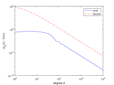
(a) $x=-0.4$

(b) $x=-0.3$

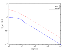
(c) $x=0.1$

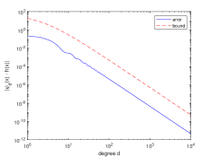
(d) $x=0.5$

Figure 1: True errors and error bounds.

4 The CJ-FEAST SVDsolver

4.1 Approximate spectral projector and its accuracy

We use the linear transformation

$$l(x)=\frac{2x-\|A\|^{2}-\sigma_{\min}^{2}}{\|A\|^{2}-\sigma_{\min}^{2}}$$ (26)

to map the spectrum interval $[\sigma_{\rm{min}}^{2},\|A\|^{2}]$ of $S=A^{T}A$ to $[-1,1]$. We remind that, to use the transformation in computation, it suffices to give rough estimates for $\|A\|$ and $\sigma_{\min}$. We can run a Lanczos, i.e., Golub–Kahan, bidiagonalization type method on $A$ several steps, say $20\sim 30$, to estimate them golub2013matrix ; jia2003implicitly ; jia2010refined , which costs very little compared to that of the CJ-FEAST SVDsolver. For a given interval $[a,b]\subset[\sigma_{\min},\|A\|]$, define the step function

$$h(x)=\begin{cases}1,\quad x\in(l(a^{2}),l(b^{2})),\\ \frac{1}{2},\quad x\in\{l(a^{2}),l(b^{2})\},\\ 0,\quad x\in[-1,1]\setminus[l(a^{2}),l(b^{2})]\end{cases}$$

and the composite function

$$f(x)=h(l(x)).$$

Therefore,

$$f(x)=\begin{cases}1,\quad x\in(a^{2},b^{2}),\\ \frac{1}{2},\quad x\in\{a^{2},b^{2}\},\\ 0,\quad x\in[\sigma_{\min}^{2},\|A\|^{2}]\setminus[a^{2},b^{2}].\end{cases}$$ (27)

Recall definition (2) of $P_{S}$. It follows from the above and (1) that

$$f(S)=Vf(\Sigma^{2})V^{T}=P_{S}.$$ (28)

Theorem 3.2 and Theorem 3.3 prove that $\psi_{d}(l(x))$ pointwise converges to $f(x)$. Correspondingly, we construct an approximate spectral projector

$$P=\psi_{d}(l(S))=\sum_{j=0}^{d}\rho_{j,d}c_{j}T_{j}(l(S)),$$ (29)

whose eigenvector matrix is $V$ and eigenvalues are $\gamma_{i}:=\psi_{d}(l(\sigma_{i}^{2}))$ with $\sigma_{i},i=1,2,\dots,n$ being the singular values of $A$. For convenience, $c_{0}$ in (29) corresponds to $\frac{c_{0}}{2}$ in (5). We see that, given a basis matrix of the subspace $\mathcal{V}^{(k-1)}$, the unique action of $P$ in Algorithm 1 is to form matrix-matrix products. We only need to store the coefficients $c_{j},\rho_{j,d},j=0,\dots,d$ without forming $P$ explicitly. We describe the computation of Chebyshev–Jackson coefficients as Algorithm 2.

Algorithm 2 The computation of Chebyshev–Jackson coefficients

0:  The matrix $A$, the interval $[a,b]$, and the series degree $d$.

0:  $c_{j},\rho_{j,d},j=0,\dots,d$.

1:  $\alpha=\arccos(l(a^{2})),\quad\beta=\arccos(l(b^{2}))$

2:  $\zeta=\frac{\pi}{d+2}$.

3:  for $j=0,1,\dots,d$ do

4:      $c_{j}=\begin{cases}\frac{\alpha-\beta}{\pi},\quad j=0,\\ \frac{2}{\pi}\frac{\sin(j\alpha)-\sin(j\beta)}{j},\quad j>0,\end{cases}$ $\rho_{j,d}=\frac{(d+2-j)\sin\zeta\cos(j\zeta)+\cos\zeta\sin(j\zeta)}{(d+2)\sin\zeta}$.

5:  end for

Next we estimate $\|P_{S}-P\|$ and the $\gamma_{i}$, which are key quantities that critically affect the convergence of the CJ-FEAST SVDsolver to be proposed and developed.

Theorem 4.1

Given the interval $[a,b]\subset[\sigma_{\min},\|A\|]$, let

$$\alpha=\arccos(l(a^{2})),\quad\beta=\arccos(l(b^{2})),$$

$$\Delta_{il}=|\arccos(l(\sigma_{il}^{2}))-\alpha|,\quad\Delta_{ir}=|\arccos(l(\sigma_{ir}^{2}))-\beta|,$$

$$\Delta_{ol}=|\arccos(l(\sigma_{ol}^{2}))-\alpha|,\quad\Delta_{or}=|\arccos(l(\sigma_{or}^{2}))-\beta|,$$

where $\sigma_{il},\ \sigma_{ir}$ and $\sigma_{ol},\ \sigma_{or}$ are the singular values of $A$ that are the closest to the ends $a$ and $b$ from inside and outside of $[a,b]$, respectively. Define

$$\Delta_{\min}={\min}\{\Delta_{il},\Delta_{ir},\Delta_{ol},\Delta_{or}\}.$$ (30)

Then

$$\|P_{S}-P\|\leq\frac{\pi^{6}}{2(d+2)^{3}\Delta_{\min}^{4}}.$$ (31)

Suppose that the singular values of $A$ in $[a,b]$ are $\sigma_{1},\ldots,\sigma_{n_{sv}}$ with $\sigma_{1},\ldots,\sigma_{r}$ in $(a,b)$ and $\sigma_{r+1},\ldots,\sigma_{n_{sv}}$ equal to $a$ or $b$ and those in $[\sigma_{\min},\|A\|]\setminus[a,b]$ are $\sigma_{n_{sv}+1},\ldots,\sigma_{n}$, and label the eigenvalues $\gamma_{i}$ of $P,\ i=1,2,\ldots,r$, $i=r+1,\ldots,n_{sv}$ and $i=n_{sv}+1,\dots,n$ in decreasing order, respectively. If

$$d\geq\frac{\sqrt[3]{2}\pi^{2}}{\Delta_{\min}^{4/3}}-2,$$ (32)

then

$$\|P_{S}-P\|<\frac{1}{4}$$ (33)

and

$$1\geq\gamma_{1}\geq\cdots\geq\gamma_{r}>\frac{3}{4}>\gamma_{r+1}\geq\cdots\geq\gamma_{n_{sv}}>\frac{1}{4}>\gamma_{n_{sv}+1}\geq\cdots\geq\gamma_{n}\geq 0.$$ (34)

Proof

Since the eigenvalues of $P_{S}$ are

$$f(\sigma_{i}^{2})=h(l(\sigma_{i}^{2}))=\begin{cases}1,\quad\sigma_{i}\in(a,b),\\ \frac{1}{2},\quad\sigma_{i}=a\mbox{ or }b,\\ 0,\quad n_{sv}+1\leq i\leq n,\end{cases}$$

from (29) we obtain

$$\|P_{S}-P\| =\|f(S)-\psi_{d}(l(S))\|=\|f(\Sigma^{2})-\psi_{d}(l(\Sigma^{2}))\|$$

$$=\max_{i=1,2,\ldots,n}|h(l(\sigma_{i}^{2}))-\psi_{d}(l(\sigma_{i}^{2}))|$$ (35)

$$=\max_{i=1,2,\ldots,n}|h(\cos(\theta_{i}))-\psi_{d}(\cos(\theta_{i}))|,$$

where $\theta_{i}=\arccos(l(\sigma_{i}^{2}))$. Note that

$$\Delta_{\min}\leq{\min}\{2\pi-2\alpha,\alpha-\beta,2\beta\}.$$

It then follows from Theorem 3.2 and Theorem 3.3 that (31) holds. It is straightforward to justify from (31) that if $d$ satisfies (32) then $\|P_{S}-P\|<\frac{1}{4}$.

It is known from Theorem 3.1 that the eigenvalues $\gamma_{i}=\psi_{d}(l(\sigma_{i}^{2})),\,i=1,2,\ldots,n$ of $P$ are in $[0,1]$, showing that $P$ is SPSD. Therefore, from (35) we obtain

$$\|P_{S}-P\|=\max\biggl{\{}\max_{\sigma_{i}\in(a,b)}1-\gamma_{i},\max_{\sigma_{i}=a\ {\rm or}\ b}\left|\frac{1}{2}-\gamma_{i}\right|,\max_{i=n_{sv}+1,\ldots,n}\gamma_{i}\biggr{\}}.$$

The above relation and (33) show that

$$0\leq 1-\gamma_{i} <\frac{1}{4},\ \sigma_{i}\in(a,b),$$

$$\left|\frac{1}{2}-\gamma_{i}\right| <\frac{1}{4},\ \sigma_{i}=a\ {\rm or}\ b,$$

$$0\leq\gamma_{i} <\frac{1}{4},\ i=n_{sv}+1,\ldots,n.$$

With the labeling order of $\gamma_{i},i=1,2,\ldots,n$, the above proves (34). ∎

Remark 1

Theorem 4.1 shows that if the approximate spectral projector has some accuracy, e.g., (33), then the dominant eigenvalues $\gamma_{1},\ldots,\gamma_{n_{sv}}$ of $P$ correspond to the desired singular values $\sigma_{1},\ldots,\sigma_{n_{sv}}$ and the associated dominant subspace are the corresponding right singular subspace. Moreover, if none of $a$ and $b$ is a singular value of $A$, then $\|P-P_{S}\|<\frac{1}{2}$ is enough to guarantee such properties. The previous example has justified that $\|P-P_{S}\|$ is reasonably small for a modest $d$; see Figure 1. In applications, we know nothing about the singular values of $A$ and $\Delta_{\min}$, and a practical selection strategy for $d$ is particularly appealing. Without a priori information on the distribution of singular values of $A$, suppose that the $\theta_{i}$ are uniformly distributed approximately, i.e., $\Delta_{\min}\approx\frac{\alpha-\beta}{n_{sv}}$. Then (32) reads as

$$d\geq\frac{\sqrt[3]{2}\pi^{2}n_{sv}^{4/3}}{(\alpha-\beta)^{4/3}}-2.$$

However, the bounds in Theorem 3.2 and Theorem 3.3, though the asymptotic convergence rates are optimal, are generally considerable overestimates, as Figure 1 has indicated. A key is that the factor $\alpha-\beta$ in the denominator that is critical and determines the accuracy of $P$; the smaller $\alpha-\beta$ is, the harder it is to approximate the step function. Therefore, we propose to choose

$$d=\left\lceil\frac{D\pi^{2}}{(\alpha-\beta)^{4/3}}\right\rceil-2$$ (36)

with $D$ some modest constant. We will propose selection strategies for choosing $D$ in (36) in subsequent algorithms.

Remark 2

As $d$ increases, $\gamma_{i}\approx 1,\ i=1,2,\ldots,r$, $\gamma_{i}\approx\frac{1}{2},\ i=r+1,\ldots,n_{sv}$, and $\gamma_{i}\approx 0,\ i=n_{sv}+1,\ldots,n$. In fact, by (31), we can make $\|P_{S}-P\|<\epsilon$ with $\epsilon$ arbitrarily small by increasing $d$. In this case, we have

$$1-\epsilon< \gamma_{i}\leq 1,i=1,2,\dots,r,$$ (37)

$$\frac{1}{2}-\epsilon< \gamma_{i}<\frac{1}{2}+\epsilon,i=r+1,\dots,n_{sv},$$ (38)

$$0\leq \gamma_{i}<\epsilon,\ i=n_{sv}+1,\ldots,n.$$ (39)

4.2 Estimates for the number of desired singular values

Note that the trace ${\rm tr}(P_{S})=r+\frac{n_{sv}-r}{2}=\frac{r+n_{sv}}{2}$, which equals $n_{sv}$ when none of $a$ and $b$ is a singular value of $A$. As Algorithm 1 requires that the subspace dimension $p\geq n_{nv}$, it is critical to reliably estimate $n_{sv}$. To this end, we first show how to choose $d$ to ensure that ${\rm tr}(P)$ approximates ${\rm tr}(P_{S})$ with an arbitrarily prescribed accuracy, and then making use of Lemma 1 to choose $p$ that ensures $p\geq n_{sv}$ reliably.

Theorem 4.2

The trace ${\rm tr}(P)$ satisfies

$$|{\rm tr}(P_{S})-{\rm tr}(P)|\leq n\|P_{S}-P\|\leq\frac{n\pi^{6}}{2(d+2)^{3}\Delta_{\min}^{4}}$$ (40)

with $\Delta_{\min}$ defined by (30).

Proof

We have

$$|{\rm tr}(P_{S})-{\rm tr}(P)| =\lvert\sum_{i=1}^{n}(f(\sigma_{i}^{2})-\gamma_{i})\rvert\leq\sum_{i=1}^{n}|f(\sigma_{i}^{2})-\gamma_{i}|$$ (41)

$$\leq n\max_{i=1,2,\ldots,n}|f(\sigma_{i}^{2})-\gamma_{i}|$$ (42)

$$=n\|P_{S}-P\|,$$

which, together with (31), proves (40). ∎

Remark 3

Bound (40) is generally very conservative since bounds (41) and (42) may be considerable overestimates by noticing that the signs of $f(\sigma_{i}^{2})-\gamma_{i}=1-\gamma_{i}\geq 0,\ i=1,2,\ldots,r$ and $f(\sigma_{i}^{2})-\gamma_{i}=-\gamma_{i}\leq 0,\ i=n_{sv}+1,\ldots,n$ are opposite, and their sizes may differ greatly. Consequently, the factor $n$ typically behaves like $\mathcal{O}(1)$, so that, in terms of Theorem 3.2 and Theorem 3.3, a modestly sized $d$ can ensure that the actual error is reasonably small.

Remark 4

Since $P$ is SPSD, we can exploit Lemma 1 to derive a reliable estimate of ${\rm tr}(P)$ and use it as an approximation to ${\rm tr}(P_{S})$. Lemma 1 indicates that the smallest sample number $M\approx\frac{8\ln\frac{2}{\delta}}{\epsilon^{2}n_{sv}}$. Note that $\epsilon\in[10^{-2},10^{-1}]$ means that $H_{M}$ is a reliable estimate for ${\rm tr}(P)$ with high probability $1-\delta\approx 1$ for $\delta\sim 10^{-2}$. For $n_{sv}$ ranging from a few to hundreds, a modest $M$ generally gives a reliable estimate for ${\rm tr}(P)$. Strikingly, for given $\epsilon$ and $\delta$, the bigger $n_{sv}$, the smaller $M$, i.e., the more easily it is to estimate a bigger $n_{sv}$.

In summary, combining Remark 3 and Remark 4, we conclude that $H_{M}$ is a reliable estimate for ${\rm tr}(P_{S})$ when $M$ and $d$ are modest. Numerical experiments in Section 6 will show that taking $d$ for $D\in[2,10]$ in (36) is reliable and produces almost unchanged $H_{M}$’s. We present Algorithm 3 to estimate $n_{sv}$, where $P$ is not formed explicitly and $H_{M}$ is efficiently computed by exploiting the three term recurrence of Chebyshev polynomials. In this way, it is, though a little tedious, easy to verify that the computation of $H_{M}$ totally requires $2Md$ MVs and approximately $6Mnd$ flops, where MV denotes a matrix-vector product with $A$ or $A^{T}$.

Algorithm 3 Estimation of the number $n_{sv}$

0:  The matrix $A$, the interval $[a,b]$, the series degree $d$, and $M$ Rademacher random $n$-vectors $z_{1},z_{2},\dots,z_{M}$.

0:  Take $H_{M}$ as an estimate for $n_{sv}$.

1:  Apply Algorithm 2 to compute the Chebyshev–Jackson coefficients.

2:  Compute $H_{M}=\frac{1}{M}\sum_{i=1}^{M}z_{i}^{T}Pz_{i}=\frac{1}{M}\sum_{i=1}^{M}\sum_{j=0}^{d}\rho_{j,d}c_{j}z_{i}^{T}T_{j}(l(S))z_{i}$.

With $H_{M}$ available, we find that taking

$$p=\lceil\mu H_{M}\rceil$$ (43)

with $\mu\geq 1.1$ can ensure the subspace dimension $p\geq n_{sv}$, where $\lceil\cdot\rceil$ is the ceil function. In fact, Lemma 1 shows that $|H_{M}-{\rm tr}(P)|\leq\epsilon\ {\rm tr}(P)$ with the high probability $1-\delta\approx 1$ for a modest $M$. Therefore, $H_{M}\geq(1-\epsilon){\rm tr}(P)$ and $\mu H_{M}\geq\mu(1-\epsilon){\rm tr}(P)$. Obviously, $\mu=1.1$ ensures that $\mu(1-\epsilon)\geq 1$ with $\epsilon\leq\frac{1}{11}$. As a result, $p$ in (43) is a reliable upper bound for ${\rm tr}(P)$ with high probability when $M$ is of modest size. On the other hand, ${\rm tr}(P)$ is a good approximation to ${\rm tr}(P_{S})$ for a proper series degree $d$. Therefore, once $M$ and $d$ are suitably chosen, $p$ in (43) can ensure $p\geq n_{sv}$ with high probability. However, different $p$’s may affect the overall efficiency of the CJ-FEAST SVDsolver. We will come back to the choice of $\mu$ after we establish the convergence of the CJ-FEAST SVDsolver.

4.3 The algorithm and some details

Having determined the approximate spectral projector $P$ and the subspace dimension $p\geq n_{sv}$, we apply Algorithm 1 to $P$, and form an approximate eigenspace of $P$ associated with its $p$ dominant eigenvalues $\gamma_{i},\ i=1,2,\ldots,p$. We then take the current subspace as the right projection subspace $\mathcal{V}^{(k)}$, form the left projection subspace $\mathcal{U}^{(k)}=A\mathcal{V}^{(k)}$, and project $A$ onto them to compute Ritz approximations $(\hat{\sigma}_{i}^{(k)},\hat{u}_{i}^{(k)},\hat{v}_{i}^{(k)})$ of the desired $n_{sv}$ singular triplets $(\sigma_{i},u_{i},v_{i})$, $i=1,2,\ldots,n_{sv}$. Precisely, let the columns of $Q_{1}^{(k)}\in\mathbb{R}^{n\times p}$ form an orthogonal basis of $\mathcal{V}^{(k)}$ and $AQ_{1}^{(k)}=Q_{2}^{(k)}\bar{A}^{(k)}$ be the thin QR factorizations of $AQ_{1}^{(k)}$, where $\bar{A}^{(k)}\in\mathbb{R}^{p\times p}$ is upper triangular. Then the columns of $Q_{2}^{(k)}$ form orthonormal basis of $\mathcal{U}^{(k)}=A\mathcal{V}^{(k)}$, and $(Q_{2}^{(k)})^{T}AQ_{1}^{(k)}=\bar{A}^{(k)}$ is the projection matrix. We describe the procedure as Algorithm 4. The computational cost of one iteration of Algorithm 4 is listed in Table 1, where, at Step 7, we exploit the fact that the upper part of the residual of $(\hat{\sigma}_{i}^{(k)},\hat{u}_{i}^{(k)},\hat{v}_{i}^{(k)})$ is zero and we do not compute it.

Algorithm 4 The CJ-FEAST SVDsolver

0:  The matrix $A$, the interval $[a,b]$, the series degree $d$, and an $n$-by-$p$ column orthonormal matrix $\hat{V}^{(0)}$ with $p\geq n_{sv}$.

0:  The $n_{sv}$ converged Ritz triplets $(\hat{\sigma}_{i}^{(k)},\hat{u}_{i}^{(k)},\hat{v}_{i}^{(k)})$ with $\hat{\sigma}_{i}^{(k)}\in[a,b]$.

1:  Apply Algorithm 2 to compute the Chebyshev–Jackson coefficients.

2:  for $k=1,2,\dots,$ do

3:     Compute $Y^{(k)}=P\hat{V}^{(k-1)}=\sum_{j=0}^{d}\rho_{j,d}c_{j}T_{j}(l(S))\hat{V}^{(k-1)}$.

4:     Make QR factorizations, and compute the projection matrix $\bar{A}^{(k)}$:$Y^{(k)}=Q_{1}^{(k)}R_{1}^{(k)}$ and $AQ_{1}^{(k)}=Q_{2}^{(k)}\bar{A}^{(k)}$.

5:     Compute the SVD: $\bar{A}^{(k)}=\bar{U}^{(k)}\hat{\Sigma}^{(k)}(\bar{V}^{(k)})^{T}$ with $\hat{\Sigma}^{(k)}={\rm diag}(\hat{\sigma}_{1}^{(k)},\ldots,\hat{\sigma}_{p}^{(k)})$.

6:     Form the approximate left and right singular vector matrices $\hat{U}^{(k)}=Q_{2}^{(k)}\bar{U}^{(k)}$ and $\hat{V}^{(k)}=Q_{1}^{(k)}\bar{V}^{(k)}$.

7:     Pick up $\hat{\sigma}_{i}^{(k)}\in[a,b]$, compute the residual norms of the Ritz approximations $(\hat{\sigma}_{i}^{(k)},\hat{u}_{i}^{(k)},\hat{v}_{i}^{(k)})$, where $\hat{u}_{i}^{(k)}=\hat{U}^{(k)}e_{i}$ and $\hat{v}_{i}^{(k)}=\hat{V}^{(k)}e_{i}$, and test convergence.

8:  end for

Table 1: Computational cost of one iteration of Algorithm 4.

Steps	MVs	flops
3	$2dp$	$4npd$
4	$p$	$2(m+n)p^{2}$
5		$21p^{3}$
6		$2(m+n)p^{2}$
7	$p$	$2np$
Total cost	$2(d+1)p$	$4ndp+4(m+n)p^{2}+2np+21p^{3}$

Suppose that $A$ is sparse and has $\mathcal{O}(m+n)$ nonzero entries, and take the subspace dimension $p=\mathcal{O}(n_{sv})$ with the constant in $\mathcal{O}(\cdot)$ comparable to but bigger than one. Then from the table we see that $2(d+1)p$ MVs cost $\mathcal{O}(2(m+n)dn_{sv})$ flops and $4ndp+4(m+n)p^{2}+2np+21p^{3}=\mathcal{O}(ndn_{sv})+\mathcal{O}((m+n)n_{sv}^{2})$. Therefore, the flops of MVs is comparable to the other cost when $d\geq\mathcal{O}(n_{sv})$. If $A$ is not sparse and non-structured, i.e., the number of its nonzero entries is $\mathcal{O}(mn)$, then MVs cost $\mathcal{O}(2mndp)$ flops and overwhelm the others unconditionally. As a result, we can measure the overall efficiency of Algorithm 4 by MVs.

5 Convergence of the CJ-FEAST SVDsolver

This section is devoted to a convergence analysis of Algorithm 4. We will establish several convergence results on the solver.

Recall from (1) that the columns of $V$ are the right singular vectors of $A$. We partition $V=[V_{p},V_{p,\perp}]$, and set up the following notation:

$$V_{p} =[v_{1},\dots,v_{p}],\ \ V_{p,\perp}=[v_{p+1},\dots,v_{n}],$$ (44)

$$\Gamma_{p} =\operatorname{diag}(\gamma_{1},\dots,\gamma_{p}),\ \ \Gamma_{p}^{\prime}=\operatorname{diag}(\gamma_{p+1},\dots,\gamma_{n}),$$ (45)

$$\Sigma_{p} =\operatorname{diag}(\sigma_{1},\dots,\sigma_{p}),\ \ \Sigma_{p}^{\prime}=\operatorname{diag}(\sigma_{p+1},\dots,\sigma_{n}).$$ (46)

It is easy to see that Algorithm 4 generates the subspaces

$${\rm span}\{\hat{V}^{(k)}\}={\rm span}\{Q_{1}^{(k)}\}={\rm span}\{Y^{(k)}\}=P{\rm span}\{\hat{V}^{(k-1)}\},$$

showing that

$${\rm span}\{\hat{V}^{(k)}\}=P^{k}{\rm span}\{\hat{V}^{(0)}\}.$$ (47)

Theorem 5.1

Suppose that $V_{p}^{T}\hat{V}^{(0)}$ is invertible and $\gamma_{p}>\gamma_{p+1}$. Then

$$Q_{1}^{(k)}=(V_{p}+V_{p,\perp}E^{(k)})(M^{(k)})^{-\frac{1}{2}}U^{(k)}$$ (48)

with

$$E^{(0)}=V_{p,\perp}^{T}\hat{V}^{(0)}(V_{p}^{T}\hat{V}^{(0)})^{-1},\ E^{(k)}=\Gamma_{p}^{\prime k}E^{(0)}\Gamma_{p}^{-k},$$ (49)

$$M^{(k)}=I+(E^{(k)})^{T}E^{(k)}$$ (50)

and $U^{(k)}$ being an orthogonal matrix; furthermore,

$$\|E^{(k)}\|\leq\biggl{(}\frac{\gamma_{p+1}}{\gamma_{p}}\biggr{)}^{k}\|E^{(0)}\|,$$ (51)

and the distance $\epsilon_{k}:={\rm dist}({\rm span}\{Q_{1}^{(k)}\},{\rm span}\{V_{p}\})$ between ${\rm span}\{Q_{1}^{(k)}\}$ and ${\rm span}\{V_{p}\}$ (cf. (golub2013matrix, , Section 2.5.3)) satisfies

$$\epsilon_{k}=\frac{\|E^{(k)}\|}{\sqrt{1+\|E^{(k)}\|^{2}}}\leq\biggl{(}\frac{\gamma_{p+1}}{\gamma_{p}}\biggr{)}^{k}\|E^{(0)}\|.$$ (52)

Label $\hat{\sigma}_{1}^{(k)},\dots,\hat{\sigma}_{p}^{(k)}$ in the same order as $\sigma_{1},\dots,\sigma_{p}$ in Theorem 4.1. Then

$$|(\hat{\sigma}_{i}^{(k)})^{2}-\sigma_{i}^{2}|\leq\|A\|^{2}(3\epsilon_{k}^{2}+\epsilon_{k}^{4}),\ i=1,2,\ldots,n_{sv}.$$ (53)

Proof

Expand $\hat{V}^{(0)}$ as the orthogonal direct sum of $V_{p}$ and $V_{p,\perp}$. Then

$$\hat{V}^{(0)}=V_{p}V_{p}^{T}\hat{V}^{(0)}+V_{p,\perp}V_{p,\perp}^{T}\hat{V}^{(0)}=(V_{p}+V_{p,\perp}V_{p,\perp}^{T}\hat{V}^{(0)}(V_{p}^{T}\hat{V}^{(0)})^{-1})V_{p}^{T}\hat{V}^{(0)}.$$

From this and the first relation in (49) it follows that

$$\hat{V}^{(0)}(V_{p}^{T}\hat{V}^{(0)})^{-1}=V_{p}+V_{p,\perp}E^{(0)}.$$

By $PV_{p}=V_{p}\Gamma_{p}$ and $PV_{p,\perp}=V_{p,\perp}\Gamma_{p}^{\prime}$, we obtain $P^{k}V_{p}=V_{p}\Gamma_{p}^{k}$ and $P^{k}V_{p,\perp}=V_{p,\perp}\Gamma_{p}^{\prime k}$. Therefore,

$$P^{k}\hat{V}^{(0)}(V_{p}^{T}\hat{V}^{(0)})^{-1}\Gamma_{p}^{-k} =V_{p}+P^{k}V_{p,\perp}E^{(0)}\Gamma_{p}^{-k}$$

$$=V_{p}+V_{p,\perp}\Gamma_{p}^{\prime k}E^{(0)}\Gamma_{p}^{-k}=V_{p}+V_{p,\perp}E^{(k)}$$ (54)

with $E^{(k)}$ defined by (49). It is straightforward that

$$\|E^{(k)}\|\leq\biggl{(}\frac{\gamma_{p+1}}{\gamma_{p}}\biggr{)}^{k}\|E^{(0)}\|,$$

which is (51). By (54), we obtain

$${\rm span}\{Q_{1}^{(k)}\}=P^{k}{\rm span}\{\hat{V}^{(0)}\}={\rm span}\{V_{p}+V_{p,\perp}E^{(k)}\}.$$

Since $Q_{1}^{(k)}$ is column orthonormal, we can express $Q_{1}^{(k)}$ as

$$Q_{1}^{(k)}=(V_{p}+V_{p,\perp}E^{(k)})(M^{(k)})^{-\frac{1}{2}}U^{(k)},$$

which establishes (48), where

$$M^{(k)}=(V_{p}+V_{p,\perp}E^{(k)})^{T}(V_{p}+V_{p,\perp}E^{(k)})=I+(E^{(k)})^{T}E^{(k)}$$

is the matrix in (50) and $U^{(k)}$ is an orthogonal matrix.

By the distance definition (golub2013matrix, , Section 2.5.3) of two subspaces, from (48) we have

$$\epsilon_{k}=\|V_{p,\perp}^{T}Q_{1}^{(k)}\|=\|E^{(k)}(M^{(k)})^{-1/2}U^{(k)}\|=\frac{\|E_{k}\|}{\sqrt{1+\|E_{k}\|^{2}}},$$

which, together with (51), proves (52).

Exploiting (1) and (48), we obtain

$$\|U^{(k)}(Q_{1}^{(k)})^{T}SQ_{1}^{(k)}(U^{(k)})^{T}-\Sigma_{p}^{2}\|$$

$$=\|(M^{(k)})^{-1/2}(V_{p}^{T}+(E^{(k)})^{T}V_{p,\perp}^{T})V\Sigma^{2}V^{T}(V_{p}+V_{p,\perp}E^{(k)})(M^{(k)})^{-1/2}-\Sigma_{p}^{2}\|$$

$$=\|(M^{(k)})^{-1/2}(\Sigma_{p}^{2}+(E^{(k)})^{T}(\Sigma_{p}^{\prime})^{2}E^{(k)})(M^{(k)})^{-1/2}-\Sigma_{p}^{2}\|$$

$$\leq\|(M^{(k)})^{-1/2}\Sigma_{p}^{2}(M^{(k)})^{-1/2}-\Sigma_{p}^{2}\|+\|(M^{(k)})^{-1/2}(E^{(k)})^{T}(\Sigma_{p}^{\prime})^{2}E^{(k)}(M^{(k)})^{-1/2}\|.$$

Let $F^{(k)}=I-(M^{(k)})^{-\frac{1}{2}}.$ Then

$$\|F^{(k)}\|=\|I-(M^{(k)})^{-\frac{1}{2}}\|=1-\frac{1}{\sqrt{1+\|E^{(k)}\|^{2}}}\leq\frac{\|E^{(k)}\|^{2}}{1+\|E^{(k)}\|^{2}}=\epsilon_{k}^{2}.$$

Therefore,

$$\|(M^{(k)})^{-1/2}\Sigma_{p}^{2}(M^{(k)})^{-1/2}-\Sigma_{p}^{2}\|=\|(I-F^{(k)})\Sigma_{p}^{2}(1-F^{(k)})-\Sigma_{p}^{2}\|$$

$$=\|-\Sigma_{p}^{2}F^{(k)}-F^{(k)}\Sigma_{p}^{2}+F^{(k)}\Sigma_{p}^{2}F^{(k)}\|\leq\|\Sigma_{p}^{2}\|(2\epsilon_{k}^{2}+\epsilon_{k}^{4}),$$

which, together with

$$\|(M^{(k)})^{-1/2}(E^{(k)})^{T}(\Sigma_{p}^{\prime})^{2}E^{(k)}(M^{(k)})^{-1/2}\|\leq\|A\|^{2}\epsilon_{k}^{2},$$

yields

$$\|U^{(k)}(Q_{1}^{(k)})^{T}SQ_{1}^{(k)}(U^{(k)})^{T}-\Sigma_{p}^{2}\|\leq\|A\|^{2}(3\epsilon_{k}^{2}+\epsilon_{k}^{4}).$$

Since the eigenvalues of $U^{(k)}(Q_{1}^{(k)})^{T}SQ_{1}^{(k)}(U^{(k)})^{T}$ are $(\hat{\sigma}_{i}^{(k)})^{2},\ i=1,2,\ldots,p$, by a standard perturbation result (golub2013matrix, , Corollary 8.1.6), the above relation leads to (53). ∎

The following theorem establishes convergence results on the Ritz vectors $\hat{u}_{i}^{(k)}$ and $\hat{v}_{i}^{(k)}$ and a new convergence result on the Ritz values $\hat{\sigma}_{i}^{(k)}$.

Theorem 5.2

Let $\beta^{(k)}=\|P^{(k)}S(I-P^{(k)})\|$, where $P^{(k)}$ is the orthogonal projector onto span$\{Q_{1}^{(k)}\}$. Assume that each singular value of $A$ in $[a,b]$ is simple, and define

$$\delta_{i}^{(k)}=\underset{j\neq i}{\min}|\sigma_{i}^{2}-(\hat{\sigma}_{j}^{(k)})^{2}|,\ i=1,2,\ldots,n_{sv}.$$ (55)

Then for $i=1,2,\dots,n_{sv}$ it holds that

$$\sin\angle(\hat{v}_{i}^{(k)},v_{i}) \leq\sqrt{1+\frac{(\beta^{(k)})^{2}}{(\delta_{i}^{(k)})^{2}}}\biggl{(}\frac{\gamma_{p+1}}{\gamma_{i}}\biggr{)}^{k}\|E^{(0)}\|,$$ (56)

$$\sin\angle(\hat{u}_{i}^{(k)},u_{i}) \leq\frac{\|A\|}{\hat{\sigma}_{i}^{(k)}}\sin\angle(\hat{v}_{i}^{(k)},v_{i}),$$ (57)

$$|(\hat{\sigma}_{i}^{(k)})^{2}-\sigma_{i}^{2}| \leq\|A\|^{2}\sin^{2}\angle(\hat{v}_{i}^{(k)},v_{i}).$$ (58)

Proof

Note that $((\hat{\sigma}_{i}^{(k)})^{2},\hat{v}_{i}^{(k)})$, $1\leq i\leq n_{sv}$ are the Ritz pairs of $S$ with respect to ${\rm span}\{Q_{1}^{(k)}\}$. Applying (saad2011numerical, , Theorem 4.6, Proposition 4.5) to our case yields

$$\sin\angle(\hat{v}_{i}^{(k)},v_{i}) \leq\sqrt{1+\frac{(\beta^{(k)})^{2}}{(\delta_{i}^{(k)})^{2}}}\sin\angle(v_{i},{\rm span}\{Q_{1}^{(k)}\}),$$ (59)

$$|(\hat{\sigma}_{i}^{(k)})^{2}-\sigma_{i}^{2}| \leq\|S-\sigma_{i}^{2}I\|\sin^{2}\angle(\hat{v}_{i}^{(k)},v_{i})\leq\|A\|^{2}\sin^{2}\angle(\hat{v}_{i}^{(k)},v_{i}),$$

which proves (58).

From (48) and (45), we obtain

$$\sin\angle(v_{i},{\rm span}\{Q_{1}^{(k)}\}) =\sin\angle(v_{i},{\rm span}\{Q_{1}^{(k)}(U^{(k)})^{T}(M^{(k)})^{1/2}\})$$

$$=\sin\angle(v_{i},V_{p}+V_{p,\perp}E^{(k)})\leq\sin\angle(v_{i},v_{i}+V_{p,\perp}E^{(k)}e_{i})$$

$$=\frac{\|E^{(k)}e_{i}\|}{\sqrt{1+\|E^{(k)}e_{i}\|^{2}}}\leq\|E^{(k)}e_{i}\|$$

$$=\|\Gamma_{p}^{\prime k}E^{(0)}\Gamma_{p}^{-k}e_{i}\|\leq\|\Gamma_{p}^{\prime k}E^{(0)}\|\gamma_{i}^{-k}$$

$$\leq\biggl{(}\frac{\gamma_{p+1}}{\gamma_{i}}\biggr{)}^{k}\|E^{(0)}\|.$$

In terms of the notation in Steps 3–5 of Algorithm 4, we have

$$\hat{U}^{(k)}\hat{\Sigma}^{(k)}=Q_{2}^{(k)}\bar{U}^{(k)}\hat{\Sigma}^{(k)}=Q_{2}^{(k)}\bar{A}^{(k)}\bar{V}^{(k)}=AQ_{1}^{(k)}\bar{V}^{(k)}=A\hat{V}^{(k)},$$

showing that

$$A\hat{v}_{i}^{(k)}=\hat{\sigma}_{i}^{(k)}\hat{u}_{i}^{(k)}.$$ (60)

Decompose $\hat{v}_{i}^{(k)}$ into the orthogonal direct sum:

$$\hat{v}_{i}^{(k)}=v_{i}\cos\angle(\hat{v}_{i}^{(k)},v_{i})+z\sin\angle(\hat{v}_{i}^{(k)},v_{i}),$$

where $z$ is orthogonal to $v_{i}$ with $\|z\|=1$. Abbreviate $\angle(\hat{v}_{i}^{(k)},v_{i})$ as $\phi_{i}$. Then

$$\hat{\sigma}_{i}^{(k)}\hat{u}_{i}^{(k)}=A\hat{v}_{i}^{(k)}=A(v_{i}\cos\phi_{i}+z\sin\phi_{i})=\sigma_{i}u_{i}\cos\phi_{i}+Az\sin\phi_{i}.$$ (61)

Since

$$u_{i}^{T}Az=z^{T}A^{T}u_{i}=\sigma_{i}z^{T}v_{i}=0,$$

it follows from (61) that

$$\sin\angle(\hat{u}_{i}^{(k)},u_{i})=\frac{\|Az\|}{\hat{\sigma}_{i}^{(k)}}\sin\phi_{i}\leq\frac{\|A\|}{\hat{\sigma}_{i}^{(k)}}\sin\phi_{i},$$

which proves (57). ∎

This theorem indicates that, provided that $\delta_{i}^{(k)}$ defined by (55) is uniformly bounded from below with respect to iteration $k$, the left and right Ritz vectors $\hat{u}_{i}^{(k)}$ and $\hat{v}_{i}^{(k)}$ converge at least with the linear convergence factor $\frac{\gamma_{p+1}}{\gamma_{i}}$ but the Ritz value $\hat{\sigma}_{i}^{(k)}$ converges at least with the factor $(\frac{\gamma_{p+1}}{\gamma_{i}})^{2}$. This indicates that the errors of the Ritz values are roughly the squares of those of the corresponding left and right Ritz vectors.

Remark 5

The slowest convergence factor $\frac{\gamma_{p+1}}{\gamma_{n_{sv}}}$ is affected by the series degree $d$ and the subspace dimension $p$. Increasing $d$ or $p$ will make this factor smaller, but will consume more computational cost in one iteration (cf. Table 1). For a modestly sized $d$, increasing $p$ will reduce the number of iterations; for $d$ very large, increasing $p$ does not reduce the number of iterations essentially since, for a very good approximate spectral projector $P$, the solver will converge in very few iterations. Numerical experiments in Section 6 will illustrate that choosing $d$ as (36) with $D\in[2,10]$ and $p$ as (43) with $\mu\in[1.1,1.5]$ is reliable and works well.

6 Numerical experiments

We now report numerical experiments, and provide a detailed numerical justification of Algorithm 3 and Algorithm 4, the theoretical results and remarks. The test matrices are from davis2011university , and we list some of their basic properties and the interval $[a,b]$ of interest in Table 2. As we see, the matrices $A$ range from rank deficient to well conditioned, and the locations of intervals and the widths relative to the whole singular spectra differ considerably. We will also find that the numbers $n_{sv}$’s of the desired singular triplets differ greatly too. Therefore, our concerning SVD problems are representative in applications, implying that our test results and assertions are of generality.

In the experiments, an approximate singular triplet $(\hat{\sigma},\hat{u},\hat{v})$ is claimed to have converged if the residual norm satisfies

$$\|r(\hat{\sigma},\hat{u},\hat{v})\|\leq\|A\|\cdot tol.$$ (62)

We will use $tol=1e-8$ and $1e-12$ to test first ten examples and $tol=1e-13$ to test the last example.

All the numerical experiments were performed on an Intel Core i7-9700, CPU 3.0GHz, 8GB RAM using MATLAB R2022a with the machine precision $\epsilon_{{\rm mach}}=2.22e-16$ under the Microsoft Windows 10 64-bit system. To make a fair comparison, for each test problem and given the subspace dimension $p$, we used the same starting $n\times p$ orthonormal $\hat{V}^{(0)}$ in all the algorithms, which is obtained by the thin QR decomposition of a random matrix generated in a normal distribution.

Table 2: Properties of test matrices, where the $nnz(A)$ is the number of nonzero entries in $A$, and the largest and smallest singular values $\|A\|$ and $\sigma_{\min}(A)$ of $A$ are from davis2011university .

Matrix $A$	$m$	$n$	$nnz(A)$	$\|A\|$	$\sigma_{\min}(A)$	$[a,b]$
GL7d12	8899	1019	37519	14.4	0	$[11,12]$
plat1919	1919	1919	32399	2.93	0	$[2.1,2.5]$
flower_5_4	5226	14721	43942	5.53	$3.70e-1$	$[4.1,4.3]$
fv1	9604	9604	85264	4.52	$5.12e-1$	$[3.1,3.15]$
3elt_dual	9000	9000	26556	3.00	$6.31e-13$	$[1.5,1.6]$
rel8	345688	12347	821839	18.3	0	$[13,14]$
crack_dual	20141	20141	60086	3.00	$1.73e-4$	$[1,1.1]$
nopoly	10774	10774	70842	23.3	$1.91e-15$	$[12,12.5]$
barth5	15606	15606	61484	4.23	$7.22e-11$	$[1.5,1.6]$
L-9	17983	17983	71192	4.00	0	$[1.2,1.3]$
shuttle_eddy	10429	10429	103599	16.2	0	$[7,7.01]$

6.1 Estimations of the number of desired singular values

We first justify that our estimates for $n_{sv}$’s are reliable. The exact singular values and $n_{sv}$’s are from davis2011university . For each test problem, we take the polynomial degree $d$ in (36) using $D=2,4,8$, compute $H_{M}$ for two modestly sized $M=20,30$, and list them in Table 3. We see that, for each problem, all the $H_{M}$ are accurate estimates for $n_{sv}$, and they remain almost unchanged. These results demonstrate that our selection strategy $D\in[2,10],M\in[20,30]$ is reliable. We suggest to use the smaller $M=20$ and the smallest $D=2$, which cost the least. Moreover, the numerical results indicates that the subspace dimension $p=\lceil 1.1H_{M}\rceil\geq n_{sv}$, which illustrates that our selection strategy (43) with $\mu\geq 1.1$ is reliable to guarantee that $p\geq n_{sv}$ in computations.

Table 3: The exact $n_{sv}$ and their estimates $H_{M}$.

Matrix	$n_{sv}$	$M$	$H_{M}$
			$D=2$	$D=4$	$D=8$
GL7d12	17	$20$	18.2	18.1	17.5
		$30$	16.9	17.6	18.5
plat1919	8	$20$	7.2	7.8	8.0
		$30$	9.2	8.4	8.4
flower_5_4	137	$20$	129.3	127.3	131.4
		$30$	131.0	133.4	135.4
fv1	89	$20$	93.4	93.8	92.1
		$30$	90.8	91.8	89.4
3elt_dual	368	$20$	360.4	354.3	374.5
		$30$	368.4	370.7	370.1
rel8	13	$20$	11.8	13.5	12.7
		$30$	14.1	11.8	12.7
crack_dual	330	$20$	333.2	331.0	329.0
		$30$	335.7	333.8	330.6
nopoly	340	$20$	335.3	336.1	347.3
		$30$	345.2	337.7	337.9
barth5	384	$20$	373.7	382.0	372.1
		$30$	388.0	382.6	380.9
L-9	477	$20$	486.2	483.3	480.9
		$30$	479.8	484.6	481.4
shuttle_eddy	6	$20$	5.6	5.7	6.4
		$30$	6.7	6.1	7.3

6.2 The case that the subspace dimension is smaller than the number of desired singular values

Our theoretical results and analysis imply that Algorithm 4 with $p<n_{sv}$ should not work generally since we may have $\gamma_{i},i=1,2,\dots,p+1$ are almost equal. As a result, subspace iteration either converges extremely slowly or fails to converge. To numerically justify these predictions, we take $d=d_{0}$, the smallest integer that satisfies (32), and $p<n_{sv}$, apply Algorithm 4 to the test matrices rel8 and plat1919, and investigate the convergence behavior.

For rel8, we first take $p=n_{sv}=13$. We observe that Algorithm 4 converges very fast and all the thirteen desired singular triplets have been found when $k=2$. But for $p=12<n_{sv}$, the residual norms of some of the Ritz triplets do not decrease from the first iteration to $k=10$; in fact, the smallest relative residual norms among the twelve ones stabilize around $3.43e-5$.

We have observed similar phenomena for plat1919. For $p=n_{sv}=8$, all the eight Ritz triplets have converged when $k=2$. But for $p=6<n_{sv}$, the algorithm fails, and the residual norms of some Ritz triplets almost stagnate from the first iteration to $k=20$, and the smallest relative residual norms stabilize around $9.10e-3$. Figure 2 depicts the convergence processes of the smallest relative residual norms for re18 and plat1919, where the residual norms stagnate from the first iteration onwards. Therefore, to make the algorithm work, one must take $p\geq n_{sv}$.

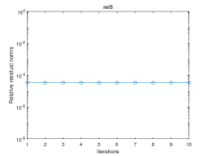
(a) rel8

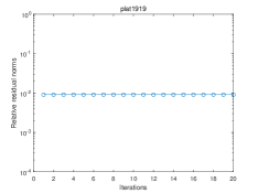
(b) plat1919

Figure 2: Convergence processes when $p<n_{sv}$.

Very importantly, our analysis and numerical justification enable us to detect if $p\geq n_{sv}$ is met: for a reasonably big $d$, if the algorithm converges extremely slowly, then it is very possible that $p<n_{sv}$; we must stop the algorithm, choose a bigger $p\geq n_{sv}$ to ensure the convergence, and find the $n_{sv}$ desired singular triplets.

6.3 Semi-definiteness of the approximate spectral projector and its accuracy

We have proved the eigenvalues $\gamma_{i}\in[0,1]$ of the approximate spectral projector $P$ in Section 4. We now confirm this property numerically and get more insights into sizes of the $\gamma_{i}$.

For GL7d12, by davis2011university , it is known that the right-most and left-most singular values in the interval $[11,12]$ are the 18-th largest one and the 34-th largest one, respectively. For flower_5_4, the right-most and left-most singular values in the interval $[4.1,4.3]$ are the 214-th largest one and the 350-th largest one, respectively. The ends of these two intervals are not singular values of the matrices, and the eigenvalues of the spectral projector $P_{S}$ are thus 1 and 0. We choose $d$ in (36) using $D=2$ and $4$, compute the eigenvalues $\gamma_{i},\ i=1,2,\ldots,n$ of $P$, and depict the eigenvalues $\gamma_{i}$ of $P$ corresponding to $\sigma_{i}\in[a,b]$ and some neighbors outside in Figure 3. We record the key quantities $\|P_{S}-P\|$, $\gamma_{n_{sv}}$ and $\gamma_{n_{sv}+1}$, the largest $\gamma_{1}$ and smallest $\gamma_{n}$, and $\gamma_{p+1}$ for $p=\lceil\mu H_{M}\rceil$ by taking $\mu=1.1,1.3,1.5$, respectively, and list them in Table 4.

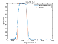
(a) GL7d12, $D=2$

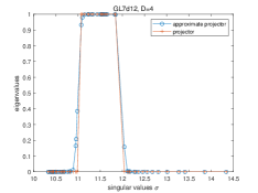
(b) GL7d12, $D=4$

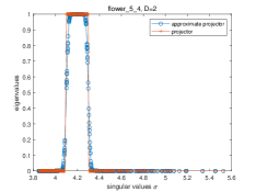
(c) flower_5_4, $D=2$

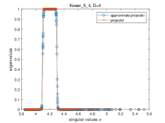
(d) flower_5_4, $D=4$

Figure 3: The partial eigenvalues of $P$.

Table 4: $\|P_{S}-P\|$ and some eigenvalues of $P$. The series degree $d$ for GL7d12 are $137$ and $276$, and the series degree $d$ for flower_5_4 are 365 and 732.

Matrix	$D$	$\|P_{S}-P\|$	$\gamma_{1}$	$\gamma_{n_{sv}}$	$\gamma_{n_{sv}+1}$	$\gamma_{p+1}$			$\gamma_{n}$
						$\mu=1.1$	$\mu=1.3$	$\mu=1.5$
GL7d12	$2$	0.4420	0.9990	0.7664	0.4420	$3.15e-1$	$9.75e-2$	$2.70e-2$	$1.63e-7$
	$4$	0.3852	0.9999	0.9323	0.3852	$1.65e-2$	$3.71e-3$	$2.02e-3$	$2.13e-8$
flower_5_4	$2$	0.4736	0.9996	0.5264	0.3978	$1.45e-1$	$7.92e-3$	$1.95e-3$	$5.28e-9$
	$4$	0.4472	0.9999	0.5528	0.3017	$1.30e-2$	$6.84e-4$	$1.93e-4$	$6.72e-10$

Several comments are in order on the figure and the table. First, for each matrix, the two $P$ generated by the two $D$ are all SPSD since all the $\gamma_{n}>0$. Second, the eigenvalues of each $P$ are indeed in $[0,1]$ since all the $\gamma_{1}<1$ and are close to one; $\|P_{S}-P\|<\frac{1}{2}$, and $\|P_{S}-P\|=1-\gamma_{n_{sv}}$ or $\gamma_{n_{sv}+1}$. Third, the $\gamma_{i}$ decay to zero fast outside the given interval, and their sizes indeed differ greatly as $i$ increases, which justifies Remark 3. Fourth, the bigger $D$ is, the larger $\gamma_{n_{sv}}$ but the smaller $\gamma_{n_{sv}+1}$ and $\gamma_{p}$ are, meaning that the algorithm converges faster as $D$, i.e., the series degree $d$, increases. Observe from (36) that $d+2$ is exactly a multiple of $D$. Insightfully, by a careful comparison, we have found that, for $D=4$, the corresponding $\gamma_{p+1}$ and $\gamma_{n}$ are approximately reduced by eight times, compared to those for $D=2$. They indicate that these quantities are approximately proportional to $1/(d+2)^{3}$, and thus numerically justified Remark 2. Fifth, for each $D$, the slowest convergence factor $\frac{\gamma_{p+1}}{\gamma_{n_{sv}}}<\frac{\gamma_{n_{sv}+1}}{\gamma_{n_{sv}}}$ considerably as $\mu$, i.e., $p$, increases, which shows that increasing $p$ can speed up the convergence of the CJ-FEAST SVDsolver considerably. Sixth, all the $\frac{\gamma_{p+1}}{\gamma_{n_{sv}}}<1$ considerably for the given $\mu\in[1.1,1.5]$ and $D=2,4$, which implies that the algorithm converges quite quickly. Visually, we plot the seven eigenvalues in Table 4 as Figure 4, and show how different they are for the two $D$. As is seen, the three $\gamma_{p+1}$ and $\gamma_{n}$ are reduced roughly one order from $D=2$ to $D=4$.

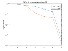
(a) GL7d12, some eigenvalues of $P$

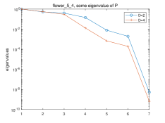
(b) flower_5_4, seven eigenvalue of $P$

Figure 4: Seven eigenvalues of $P$

The above results and analysis indicate that $\mu\in[1.1,1.5]$ for a small $D$ are practical and work well.

6.4 A comparison of CJ-FEAST SVDsolver and IFEAST

In this subsection we numerically compare Algorithm 4 with the contour integral-based FEAST algorithm with inexact linear system solves, abbreviated as IFEAST gavin2018ifeast ; polizzi2020feast , which can be directly adapted to the SVD problem under consideration. We use IFEAST to construct $P$ and then use Algorithm 1. The unique fundamental difference between Algorithm 4 and IFEAST is the construction way of $P$, and all the other steps are the same.

IFEAST can use some flexible parameters (polizzi2020feast, , Section 3.1), such as different contours and numerous numerical quadrature rules. Here, for a given interval $[a,b]$ of interest, we use the circle with the center $\frac{a^{2}+b^{2}}{2}$ and radius $\frac{b^{2}-a^{2}}{2}$ as the contour. We use the trapezoidal rule with eight nodes and the Gauss–Legendre quadrature with sixteen nodes on the circle, respectively, which are default parameters in (polizzi2020feast, , Section 3.1) and are also used in tang2014feast and guttel2015zolotarev . At each iteration, the resulting shifted linear systems are solved by BiCGstab, as suggested in polizzi2020feast , with increasing accuracy and the parameter $\alpha=0.01$ (gavin2018ifeast, , Section 2), and the maximum iteration number is set to $n$, i.e., the problem size of shifted linear systems.

Notice that $A^{T}A$ is real symmetric and the quadrature nodes are symmetric with respect to the real axis, IFEAST only needs to solve $p\times\frac{nnode}{2}$ linear systems at each subspace iteration step, where $nnode$ is the number of nodes on the circle. As we have addressed, just as those shifted linear systems can be solved in parallel, Step 3 of the CJ-FEAST SVDsolver can be implemented in parallel too; that is, each of the $p$ matrix-vector products is computed in a separate processor. More precisely, one may solve the shifted linear systems in $p\times\frac{nnode}{2}$ processors, while the $p$ MVs in CJ–FEAST SVDsolver can be performed only in $p$ processors at each iteration. As a result, for a fair comparison, we only record the sequential MVs gavin2018ifeast , which is the sum of the most MVs that BiCGstab uses for the one among these linear systems at each subspace iteration step. Notice that, for the shifted linear systems resulting from the matrices $A^{T}A$, one iteration of BiCGstab costs four MVs with $A$ and $A^{T}$. Keep in mind that if Step 3 of Algorithm 4 is implemented in parallel then it consumes $2d$ sequential MVs for one subspace iteration step. It is fair to use the sequential MVs to measure the overall efficiency of CJ-FEAST and IFEAST.

We take the same initial $\mathcal{V}^{(0)}$ and the same subspace dimension $p$ as (43) with $\mu=1.2,1.5$, and $H_{M}$ is the closest one to $n_{sv}$ selected from Table 3. For Algorithm 4, we choose the series degree $d$ using (36) with $D=1,2,3$, respectively. We record the sequential MVs and the number of iterations $k$ that the norms of all the desired approximate singular triplets drop below a prescribed tolerance $tol$, and denote them by SeqMVs($k$). Moreover, we use the speedup ratio (SR) to compare the efficiency, where SR is equal to the ratio of the SeqMVs of IFEAST over the mean value of the three SeqMVs of Algorithm 4. Therefore, SR is the efficiency multiple of CJ-FEAST over IFEAST, and SR $>1$ indicates that Algorithm 4 is more efficient; otherwise, Algorithm 4 is less efficient. Table 5 and Table 6 list the results obtained for $tol=1e-8$ and $tol=1e-12$, respectively, where we have abbreviated the trapezoidal rule and the Gauss–Legendre quadrature as T and G, respectively.

Table 5: Computational results of IFEAST and Algorithm 4 with $tol=1e-8$.

Matrix	$p$	SeqMVs$(k)$					SR
		IFEAST		Algorithm 4			T	G
		T	G	$D=1$	$D=2$	$D=3$
GL7d12	21	2906(11)	4418(4)	2448(18)	2466(9)	2484(6)	1.2	1.8
	26	1962(8)	3630(4)	1904(14)	1370(5)	1656(4)	1.2	2.2
plat1919	10	410(7)	588(4)	756(14)	672(6)	680(4)	0.6	0.8
	12	398(7)	450(3)	756(14)	672(6)	510(3)	0.6	0.7
flower_5_4	163	9794(13)	16320(4)	5824(16)	4380(6)	4392(4)	2.0	3.3
	204	8202(7)	23336(4)	2548(7)	2920(4)	3294(3)	2.8	8.0
fv1	108	31176(8)	82318(4)	12120(6)	12132(3)	18198(3)	2.2	5.8
	135	21954(6)	58902(3)	8080(4)	12132(3)	12132(2)	2.0	5.5
3elt_dual	443	20670(16)	37450(4)	10620(18)	9472(8)	8890(5)	2.1	3.6
	553	9786(7)	30962(4)	4130(7)	4736(4)	5334(3)	2.1	6.5
rel8	16	3910(16)	3592(4)	6160(28)	4884(11)	4008(6)	0.8	0.7
	20	2458(10)	2612(3)	3300(15)	2220(5)	2672(4)	0.9	1.0
crack_dual	397	84646(25)	61700(5)	19314(29)	17368(13)	16032(8)	4.8	3.5
	496	21170(13)	52332(5)	11332(17)	8016(6)	8016(4)	2.3	5.7
nopoly	406	51228(15)	116320(5)	19008(18)	14798(7)	12696(4)	3.3	7.5
	507	20912(7)	66756(4)	5280(5)	8456(4)	9522(3)	2.7	8.6
barth5	460	101058(23)	148510(5)	18828(18)	12564(6)	12576(4)	6.9	10.1
	574	31912(8)	88370(4)	5230(5)	8376(4)	9432(3)	4.2	11.5
L-9	576	68666(16)	155076(5)	14970(15)	11988(6)	11992(4)	5.3	11.9
	720	40714(9)	91302(4)	4990(5)	7992(4)	8994(3)	5.6	12.5

Table 6: Computational results of IFEAST and Algorithm 4 with $tol=1e-12$.

Matrix	$p$	SeqMVs$(k)$					SR
		IFEAST		Algorithm 4			T	G
		T	G	$D=1$	$D=2$	$D=3$
GL7d12	21	6576(17)	7052(5)	4352(32)	4110(15)	3726(9)	1.6	1.7
	26	5312(14)	7598(7)	2992(22)	2466(9)	2070(5)	2.1	3.0
plat1919	10	666(12)	674(5)	1188(22)	1008(9)	850(5)	0.7	0.7
	12	522(10)	714(5)	1080(20)	896(8)	850(5)	0.6	0.8
flower_5_4	163	57162(20)	35764(5)	9464(26)	7300(10)	5490(5)	7.7	4.8
	204	14568(9)	26788(5)	3276(9)	3650(5)	5496(5)	3.5	6.5
fv1	108	193024(14)	195936(7)	16160(8)	20220(5)	24264(4)	9.5	9.7
	135	76036(7)	95756(4)	10100(5)	16176(4)	18198(3)	5.1	6.5
3elt_dual	443	174642(24)	109562(6)	18880(32)	13024(11)	10668(6)	12.3	7.7
	553	47492(11)	102634(6)	5310(9)	5920(5)	8890(5)	7.1	15.3
rel8	16	7998(22)	5818(5)	8140(37)	6660(15)	5344(8)	1.2	0.9
	20	5304(14)	7630(5)	4620(21)	3552(8)	3340(5)	1.4	2.0
crack_dual	397	371568(38)	225696(8)	31968(48)	25384(19)	22044(11)	14.0	8.5
	496	192250(21)	178956(7)	13986(21)	10688(8)	12024(6)	15.7	14.6
nopoly	406	314438(26)	125280(6)	26400(25)	19026(9)	19044(6)	14.6	5.8
	507	82246(10)	75062(5)	6336(6)	10570(5)	12696(4)	8.3	7.7
barth5	460	889820(39)	175112(6)	27196(26)	20940(10)	18864(6)	39.8	7.8
	574	150860(10)	113838(5)	8368(8)	10470(5)	12576(4)	14.4	10.9
L-9	576	471596(25)	193192(6)	23952(24)	19980(10)	17988(6)	22.8	9.4
	720	220778(12)	145958(6)	6986(7)	9990(5)	11992(4)	22.9	15.1

Let us analyze Table 5 and Table 6. For GL7d12, plat1919 and rel8, since the intervals of interest are close to the right end of the singular spectra, the shifted linear systems involved in IFEAST are not very indefinite by noticing that most of the eigenvalues of the coefficient matrices are in the left half plane and only a handful of them are in the right half plane. It is known that, for such linear systems, Krylov iterative solvers such as BiCGstab and GMRES may converge relatively faster. As the SR columns of tables indicate, the SeqMVs consumed by IFEAST and CJ-FEAST are comparable, meaning that the two algorithms are almost equally efficient and there is no obvious winner. But for the other seven test problems, the intervals of interest are truly inside the singular spectra, that is, the desired singular values are some relatively interior ones, so that the linear systems in the IFEAST may be highly indefinite, which make Krylov iterative solvers possibly converge very slowly. For these SVD problems, we see from the SR columns of tables that CJ-FEAST is a few and often tens times more efficient than IFEAST, very substantial improvements.

We have more findings. When the stopping tolerance $tol$ changes from $1e-8$ to $1e-12$, although the outer iterations needed increase regularly for each problem and given parameters, the SeqMVs($k$) consumed by IFEAST may increase dramatically, which are especially true when the intervals of interest are inside the singular spectra. By inspecting the convergence processes of BiCGstab for solving shifted linear systems at each outer iteration, we have observed that it became much harder for BiCGstab to reduce the residual norms of shifted systems as outer iterations proceed and approximate singular triplets converge. In fact, we have found that once outer residual norms are around $1e-11$, BiCGstab often consumed considerably many iterations to meet the desired stopping criterion in subsequent outer iterations. In contrast, CJ-FEAST always converges linearly and regularly, and the SeqMVs used by it thus increase regularly from $tol=1e-8$ to $tol=1e-12$. This can be seen from the SR columns of the tables, where CJ-FEAST is more advantageous to the two contour integral-based IFEAST solvers for $tol=1e-12$.

Finally, we test the CJ-FEAST SVDsolver and IFEAST on the problem shuttle_eddy with $tol=1e-13$, which, though smaller, is considerably bigger than $\mathcal{O}(\epsilon_{\rm mach})$. We take $p=\lceil 1.2H_{M}\rceil=\lceil 1.2\times 6.1\rceil=8$, where $H_{M}=6.1$ is the closest to $n_{sv}=6$ selected from Table 3. For IFEAST, we plot the convergence processes of the biggest relative residual norms among the six ones in Figure 5a. For CJ–FEAST with $D=1$ and 2, which corresponds to $d=64914$ and $129830$, the convergence processes of the six Ritz approximations are similar, and we plot the residual norms of one Ritz approximation with $D=1$ and $D=2$ in Figure 5a, respectively. We also take a closer look at the convergence behavior of IFEAST and plot Figure 5b after the residual norms drop below $1e-11$, which exhibits the subsequent convergence process more clearly and visually.

Several comments are made. First, it is observed from Figure 5a that both IFEAST and CJ–FEAST converge quite fast until the residual norm decreases to $1e-11$. After that, IFEAST with the trapezoidal rule starts to stabilize above $tol=1e-13$ in subsequent iterations and IFEAST with the Gauss–Legendre quadrature succeeds but converges irregularly, while CJ–FEAST with $D=1,2$ performs regularly and the residual norms drops below $tol=1e-13$ at iterations $k=3$ and $2$, respectively. Second, if $tol=1e-11$ then all the residual norms of six desired triplets computed by IFEAST with the trapezoidal rule and Gauss–Legendre quadrature drop below $1e-11$ at iterations $k=9,8$, respectively, and the SeqMVs are 361338 and 333572; the SeqMVs$(k)$ consumed by CJ–FEAST with $D=1$ and 2 are $389484(3)$ and $519320(2)$, respectively. Therefore, CJ-FEAST with $D=1$ is as efficient as IFEAST if $tol=1e-11$. Third, Figure 5b shows that IFEAST with the Gauss–Legendre quadrature behaves irregularly but the residual norm ultimately drops below the prescribed $tol=1e-13$ at $k=31$, while the residual norms obtained by IFEAST with the trapezoidal rule decrease faster and more regularly but almost stagnate from $k=15$ upwards with the residual norms bigger than $tol$. Fourth, the residual norms computed by CJ–FEAST with $D=1$ and 2 further decrease and achieve the prescribed tolerance very quickly. As a matter of fact, the residual norms of six Ritz approximations computed by CJ–FEAST with $D=1$ are already $4.64e-15,5.61e-15,4.94e-15,5.91e-15,5.87e-15,9.25e-15$ and with $D=2$ are $6.62e-15,6.07e-15,6.00e-15,6.59e-15,6.25e-15,6.36e-15$, respectively. All of them are $\mathcal{O}(\epsilon_{\rm mach})$. Therefore, for this problem, Algorithm 4 is more robust than IFEAST when higher accuracy is required. More generally, we have found that CJ-FEAST works well for a prescribed tolerance $tol=\mathcal{O}(\epsilon_{\rm mach})$, but IFEAST may fail to converge for $tol=1e-13$ or smaller but no less than $\mathcal{O}(\epsilon_{\rm mach})$ for some problems, due to the solutions of shifted linear systems in finite precision.

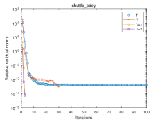
(a) convergence process

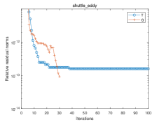
(b) A closer look

Figure 5: Convergence process of shuttle_eddy with $tol=1e-13$.

7 Conclusions

We have considered the problem of approximating the step function $h(x)$ in (4) by the Chebyshev–Jackson polynomial series, proved its pointwise convergence to $h(x)$, and derived quantitative pointwise error bounds. Making use of these results, we have established quantitative accuracy estimates for the approximate spectral projector constructed by the series as an approximation to the spectral projector $P_{S}$ of $A^{T}A$ associated with all the singular values $\sigma\in[a,b]$. We have also proved that the approximate spectral projector constructed by the Chebyshev–Jackson series is unconditionally SPSD, which enables us to reliably estimate the number $n_{sv}$ of desired singular triplets and propose a robust selection strategy to ensure that the subspace dimension $p\geq n_{sv}$. Based on these results, we have developed the CJ-FEAST SVDsolver for the computation of the singular triplets of $A$ with $\sigma\in[a,b]$. We have analyzed the convergence of the algorithm, and proved how the subspaces constructed converge to the desired right singular subspace and how each of the Ritz approximations converges as iterations proceed. In the meantime, we have discussed how to select the subspace dimension $p$ and the series degree $d$ in computations, and proposed robust and general-purpose selection strategies for them. We have numerically tested our CJ-FEAST SVDsolver on a number of problems in several aspects and shown that it is robust, effective and efficient. Numerical experiments have demonstrated that the CJ-FEAST SVDsolver is at least competitive with IFEAST and is much more efficient than IFEAST when the desired singular values are extreme and interior ones, respectively, and they have also illustrated that CJ-FEAST is more robust than IFEAST if a higher accuracy is required.

The adaptation of the CJ-FEAST SVDsolver to the real symmetric and complex Hermitian eigenvalue problem is straightforward, where the eigenpairs with the eigenvalues in a given real interval are of interest. We only need to replace the Rayleigh–Ritz projection for the SVD problem by the counterpart for the eigenvalue problem. The results and analysis are directly applicable or adaptable to the variant of SVDsolver, i.e., the CJ-FEAST eigensolver, and the practical selection strategies proposed for $p$ and $d$ still work. Moreover, the construction of an approximate spectral projector by the Chebyshev–Jackson series involves only matrix-matrix products and can thus be implemented very efficiently in parallel computing environments. In a word, the CJ-FEAST eigensolver is an efficient and robust alternative of the available contour integral-based FEAST eigensolvers for real symmetric or complex Hermitian eigenvalue problems.

Declarations

Conflict of interest  The two authors declare that they have no financial interests, and they read and approved the final manuscript. The algorithmic Matlab code is available upon reasonable request from the corresponding author.

Data Availability  Enquires about data availability should be directed to the authors.

References

- (1) Avron, H., Toledo, S.: Randomized algorithms for estimating the trace of an implicit symmetric positive semi-definite matrix. J. ACM 58(2), Art. 8, 17 (2011). DOI 10.1145/1944345.1944349
- (2) Cortinovis, A., Kressner, D.: On randomized trace estimates for indefinite matrices with an application to determinants. Found. Comput. Math. 22(3), 875–903 (2022). DOI 10.1007/s10208-021-09525-9
- (3) Davis, T.A., Hu, Y.: The University of Florida sparse matrix collection. ACM Trans. Math. Software 38(1), Art. 1, 25 (2011). DOI 10.1145/2049662.2049663
- (4) Di Napoli, E., Polizzi, E., Saad, Y.: Efficient estimation of eigenvalue counts in an interval. Numer. Linear Algebra Appl. 23(4), 674–692 (2016). DOI 10.1002/nla.2048
- (5) Futamura, Y., Sakurai, T.: z-Pares: Parallel Eigenvalue Solver (2014). URL https://zpares.cs.tsukuba.ac.jp/
- (6) Gavin, B., Polizzi, E.: Krylov eigenvalue strategy using the FEAST algorithm with inexact system solves. Numer. Linear Algebra Appl. 25(5), e2188, 20 (2018). DOI 10.1002/nla.2188
- (7) Golub, G.H., Van Loan, C.F.: Matrix Computations, fourth edn. Johns Hopkins Studies in the Mathematical Sciences. Johns Hopkins University Press, Baltimore, MD (2013)
- (8) Güttel, S., Polizzi, E., Tang, P.T.P., Viaud, G.: Zolotarev quadrature rules and load balancing for the FEAST eigensolver. SIAM J. Sci. Comput. 37(4), A2100–A2122 (2015). DOI 10.1137/140980090
- (9) Ikegami, T., Sakurai, T.: Contour integral eigensolver for non-Hermitian systems: a Rayleigh-Ritz-type approach. Taiwanese J. Math. 14(3A), 825–837 (2010). DOI 10.11650/twjm/1500405869
- (10) Ikegami, T., Sakurai, T., Nagashima, U.: A filter diagonalization for generalized eigenvalue problems based on the Sakurai-Sugiura projection method. J. Comput. Appl. Math. 233(8), 1927–1936 (2010). DOI 10.1016/j.cam.2009.09.029
- (11) Imakura, A., Du, L., Sakurai, T.: A block Arnoldi-type contour integral spectral projection method for solving generalized eigenvalue problems. Appl. Math. Lett. 32, 22–27 (2014). DOI 10.1016/j.aml.2014.02.007
- (12) Imakura, A., Du, L., Sakurai, T.: Relationships among contour integral-based methods for solving generalized eigenvalue problems. Jpn. J. Ind. Appl. Math. 33(3), 721–750 (2016). DOI 10.1007/s13160-016-0224-x
- (13) Jay, L.O., Kim, H., Saad, Y., Chelikowsky, J.R.: Electronic structure calculations for plane-wave codes without diagonalization. Comput. Phys. Commun. 118(1), 21–30 (1999). DOI 10.1016/S0010-4655(98)00192-1
- (14) Jia, Z.: Polynomial characterizations of the approximate eigenvectors by the refined Arnoldi method and an implicitly restarted refined Arnoldi algorithm. Linear Algebra Appl. 287(1-3), 191–214 (1999). DOI 10.1016/S0024-3795(98)10197-0
- (15) Jia, Z., Niu, D.: An implicitly restarted refined bidiagonalization Lanczos method for computing a partial singular value decomposition. SIAM J. Matrix Anal. Appl. 25(1), 246–265 (2003). DOI 10.1137/S0895479802404192
- (16) Jia, Z., Niu, D.: A refined harmonic Lanczos bidiagonalization method and an implicitly restarted algorithm for computing the smallest singular triplets of large matrices. SIAM J. Sci. Comput. 32(2), 714–744 (2010). DOI 10.1137/080733383
- (17) Kestyn, J., Polizzi, E., Tang, P.T.P.: FEAST eigensolver for non-Hermitian problems. SIAM J. Sci. Comput. 38(5), S772–S799 (2016). DOI 10.1137/15M1026572
- (18) Lehoucq, R.B., Sorensen, D., Yang, C.: ARPACK Users’ Guide: Solution of Large Scale Eigenvalue Problems by Implicitly Restarted Arnoldi Methods. SIAM, Philadephia, PA (1998)
- (19) Mason, J.C., Handscomb, D.C.: Chebyshev Polynomials. Chapman & Hall/CRC, Boca Raton, FL (2003)
- (20) Parlett, B.N.: The Symmetric Eigenvalue Problem, Classics in Applied Mathematics, vol. 20. SIAM, Philadelphia, PA (1998). DOI 10.1137/1.9781611971163
- (21) Polizzi, E.: Density-matrix-based algorithm for solving eigenvalue problems. Phys. Rev. B 79(11), e115112, 6 (2009). DOI 10.1103/PhysRevB.79.115112
- (22) Polizzi, E.: FEAST eigenvalue solver v4.0 user guide (2020). DOI 10.48550/arXiv.2002.04807
- (23) Rivlin, T.J.: An Introduction to the Approximation of Functions. Dover Books on Advanced Mathematics. Dover Publications, Inc., New York (1981)
- (24) Robbé, M., Sadkane, M., Spence, A.: Inexact inverse subspace iteration with preconditioning applied to non-Hermitian eigenvalue problems. SIAM J. Matrix Anal. Appl. 31(1), 92–113 (2009). DOI 10.1137/060673795
- (25) Roosta-Khorasani, F., Ascher, U.: Improved bounds on sample size for implicit matrix trace estimators. Found. Comput. Math. 15(5), 1187–1212 (2015). DOI 10.1007/s10208-014-9220-1
- (26) Saad, Y.: Iterative Methods for Sparse Linear Systems, second edn. SIAM, Philadelphia, PA (2003). DOI 10.1137/1.9780898718003
- (27) Saad, Y.: Numerical Methods for Large Eigenvalue Problems, Classics in Applied Mathematics, vol. 66. SIAM, Philadelphia, PA (2011). DOI 10.1137/1.9781611970739
- (28) Sakurai, T., Sugiura, H.: A projection method for generalized eigenvalue problems using numerical integration. J. Comput. Appl. Math. 159(1), 119–128 (2003). DOI 10.1016/S0377-0427(03)00565-X
- (29) Sakurai, T., Tadano, H.: CIRR: a Rayleigh-Ritz type method with contour integral for generalized eigenvalue problems. Hokkaido Math. J. 36(4), 745–757 (2007). DOI 10.14492/hokmj/1272848031
- (30) Sorensen, D.C.: Implicit application of polynomial filters in a -step Arnoldi method. SIAM J. Matrix Anal. Appl. 13(1), 357–385 (1992). DOI 10.1137/0613025
- (31) Stewart, G.W.: Matrix Algorithms, Vol. II: Eigensystems. SIAM, Philadelphia, PA (2001). DOI 10.1137/1.9780898718058
- (32) Tang, P.T.P., Polizzi, E.: FEAST as a subspace iteration eigensolver accelerated by approximate spectral projection. SIAM J. Matrix Anal. Appl. 35(2), 354–390 (2014). DOI 10.1137/13090866X