Attention-based Random Forest and Contamination Model
Abstract
A new approach called ABRF (the attention-based random forest) and its modifications for applying the attention mechanism to the random forest (RF) for regression and classification are proposed. The main idea behind the proposed ABRF models is to assign attention weights with trainable parameters to decision trees in a specific way. The weights depend on the distance between an instance, which falls into a corresponding leaf of a tree, and instances, which fall in the same leaf. This idea stems from representation of the Nadaraya-Watson kernel regression in the form of a RF. Three modifications of the general approach are proposed. The first one is based on applying the Huber’s contamination model and on computing the attention weights by solving quadratic or linear optimization problems. The second and the third modifications use the gradient-based algorithms for computing trainable parameters. Numerical experiments with various regression and classification datasets illustrate the proposed method.
Keywords: attention mechanism, random forest, Nadaraya-Watson regression, quadratic programming, linear programming, contamination model, classification, regression
1 Introduction
The attention mechanism can be regarded as a tool by which a neural network can automatically distinguish the relative importance of features or instances and weigh them for improving the classification or regression accuracy. It can be viewed as a learnable mask which emphasizes relevant information in a feature map. Originally, attention stems from a property of the human perception to selectively concentrate on an important part of information and to ignore other information [1]. Therefore, many applications of the attention mechanism focus on the natural language processing (NLP) models, including text classification, translation, etc. Many attention-based models are also applied to the computer vision area, including image-based analysis, visual question answering, etc. Detailed surveys and reviews of attention, its forms, properties and applications can be found in [2, 3, 4, 5, 1].
Many neural attention models are simple, scalable, flexible, and with promising results in several application domains [3]. However, attention is considered as an essential component of neural architectures [2], the attention weights are learned by incorporating an additional feed forward neural network within the architectures. This implies that they have all problems which are encountered in neural networks, including, overfitting, many tuning parameters, requirements of a large amount of data, the black-box nature, expensive computations. One of the powerful models different from neural networks is the random forest (RF) [6], which uses a large number of randomly built individual decision trees in order to combine their predictions. RFs reduce the possible correlation between decision trees by selecting different subsamples of the feature space and different subsamples of instances.
Our aim is to avoid using neural networks and to propose the attention-based random forest (ABRF) models which can be regarded as an efficient alternative to neural networks in many applications. Moreover, the ABRF models can also be an efficient alternative to the RF and enhance the RF regression and classification accuracy.
The main idea behind the proposed ABRF models is to assign weights to decision trees in a specific way. The weights can be regarded as the attention weights because they are defined by using queries, keys and values concepts in terms of the attention mechanism. In contrast to weights of trees defined in [7, 8], weights in the ABRF have trainable parameters and depend on how far an instance, which falls into a leaf, is from instances, which fall in the same leaf. The resulting prediction of the ABRF is computed as a weighted sum of predictions obtained by means of decision trees.
It is pointed out in [2, 9] that the original idea of attention can be understood from the statistics point of view applying the Nadaraya-Watson kernel regression model [10, 11]. According to the Nadaraya-Watson regression, weights or normalized kernels conform with relevance of a training instance to a target feature vector. Our idea in terms of the original attention mechanism is to consider every decision tree prediction as the value, the training instance as the key, the testing instance as the query. In fact, we combine the Nadaraya-Watson kernel regression model in the form of the RF. The most interesting question with respect to this representation is how to compute and to train weights of trees, how to define trainable parameters of the weights.
Depending on a way for the definition of weights and a way for their training, we propose the following three modifications of the ABRF models:
-
1.
ABRF-1 whose decision tree weights are learned by using the well-known Huber’s -contamination model [12] where the trainable parameters of weights are optimally selected from an arbitrarily adversary distribution. Each weight consists of two parts: the softmax operation with the tuning coefficient and the trainable bias of the softmax weight with coefficient . This is a very surprising link between robust contamination model and the attention mechanism. An advantage of using the -contamination model for training the attention weights is that the tree weights used to form prediction are linear on trainable parameters. This fact allows us to formulate optimization problem in terms of quadratic or even linear programming, i.e., we get the linear or quadratic programming problems for computing optimal weights and do not use the gradient-based algorithm for learning. The quadratic programming problem has a unique solution, and there are many efficient algorithms for its solving.
-
2.
ABRF-2 whose decision tree weights are defined in the standard way through the softmax operation where the trainable parameters are incorporated into the softmax function. This modification is more flexible because trainable parameters and the entire attention weights may be defined in various ways, for example, in conventional ways accepted in attention models [13, 14, 1, 15]. In spite of the flexibility of the modification, it requires using gradient methods for searching for optimal weights or their trainable parameters with all virtues and shortcomings of the computational methods.
-
3.
ABRF-3 is a combination of ABRF-1 and ABRF-2. The modification extends the set of trainable parameters of attention weights. We learn two subsets of parameters. The first one consists of the trainable biases in the -contamination model, the second subset includes parameters incorporated into the softmax operation. It is obvious that gradient descent methods can be used for all parameters. The third modification can be regarded as a generalization of ABRF-1 and ABRF-2.
One of the important advantages of the ABRF (ABRF-1) is that the simple quadratic or linear optimization problems have to be solved to train weights of trees. Another advantage is that we do not need to rebuild trees after appearing new training examples. It is enough to train new weights of trees. The models provide interpretable predictions because weights of trees show which decision trees have the largest contribution into predictions. There are also other advantages which will be pointed out below. To the best of our knowledge, there are no similar attention-based RF models combined with the Huber’s -contamination model. Due to their flexibility, they can be a basis for development quite a new class of attention-based models trained especially on small datasets when the original neural network models may provide worse results.
Many numerical experiments are provided for studying the proposed attention-based models. We investigate two types of RFs: original RFs and Extremely Randomized Trees (ERT). At each node, the ERT algorithm chooses a split point randomly for each feature and then selects the best split among these [16].
The paper is organized as follows. Related work can be found in Section 2. A brief introduction to the attention mechanism is given in Section 3. The proposed model and its modifications for regression are provided in Section 4. Some changes of the general model for classification are considered in Section 5. Numerical experiments illustrating regression and classification problems are provided in Section 6. Concluding and discussion remarks can be found in Section 7.
2 Related work
Attention mechanism. Many attention-based models have been developed to improve the performance of classification and regression algorithms. Surveys of various attention-based models are available in [2, 3, 4, 5, 17, 1].
It should be noted that one of the computational problems of attention mechanisms is training the softmax function. In order to overcome this difficulty, several interesting approaches have been proposed. Choromanski et al. [18] introduced Performers as a Transformer architecture which can estimate softmax attention with provable accuracy using only linear space and time complexity. A linear unified nested attention mechanism that approximates softmax attention with two nested linear attention functions was proposed by Ma et al. [19]. A new class of random feature methods for linearizing softmax and Gaussian kernels called hybrid random features (HRFs) was introduced in [20]. The same problem is solved in [21] where the authors propose random feature attention, a linear time and space attention that uses random feature methods to approximate the softmax function. Schlag et al. [22] proposed a new kernel function to linearize attention which balances simplicity and effectiveness. A detailed survey of techniques of random features to speed up kernel methods was provided by Liu et al. [17].
We propose three modifications of the attention-based RF such that the second and the third modifications (ABRF-2 and ABRF-3) have trainable softmax functions and meet computational problem to solve the corresponding optimization problems. However, the first modification (ABRF-1) is based on solving the standard linear or quadratic optimization problems. It overcomes the computational problems of the attention mechanism.
Weighted RFs. Various approaches were developed to implement the weighted random forests. Approaches of the first group are based on assigning weights to decision trees in accordance with some criteria to improve the classification and regression models [23, 24, 25, 26, 27, 28]. There are approaches [29] which use weights of classes to deal with imbalanced datasets. However, the assigned weights in the aforementioned works are not trainable parameters. Attempts to train weights of trees were carried out in [30, 31, 7, 8], where weights are assigned by solving optimization problems, i.e., they incorporated into a certain loss function of the whole RF such that the loss function is minimized over values of weights.
In contrast to the above approaches, weights assigned to trees in the proposed attention-based models depend not only on trees, but on each instance, i.e., vectors of the feature weights, the preliminary tree weights, the instance weights are introduced and learned to implement the attention mechanism. This is a very important difference of the proposed attention-based models from the available weighted RFs.
3 Preliminary: The attention mechanism
The attention mechanism can be regarded as a tool by which a neural network can automatically distinguish the relative importance of features and weigh the features for enhancing the classification accuracy. It can be viewed as a learnable mask which emphasizes relevant information in a feature map. It is pointed out in [2, 9] that the original idea of attention can be understood from the statistics point of view applying the Nadaraya-Watson kernel regression model [10, 11].
Given instances , in which represents a feature vector involving features and represents the regression outputs, the task of regression is to construct a regressor which can predict the output value of a new observation , using available data . The similar task can be formulated for the classification problem.
The original idea behind the attention mechanism is to replace the simple average of outputs for estimating the regression output , corresponding to a new input feature vector with the weighted average, in the form of the Nadaraya-Watson regression model [10, 11]:
| (1) |
where weight conforms with relevance of the -th instance to the vector .
According to the Nadaraya-Watson regression model, to estimate the output of an input variable , training outputs given from a dataset weigh in agreement with the corresponding input locations relative to the input variable . The closer an input to the given variable , the greater the weight assigned to the output corresponding to .
One of the original forms of weights is defined by a kernel (the Nadaraya-Watson kernel regression [10, 11]), which can be regarded as a scoring function estimating how vector is close to vector . The weight is written as follows:
| (2) |
In terms of the attention mechanism [13], vector , vectors and outputs are called as the query, keys and values, respectively. Weight is called as the attention weight. Generally, weights can be extended by incorporating trainable parameters. For example, if we denote and referred to as the query and key embeddings, respectively, then the attention weight can be represented as:
| (3) |
where and are matrices of parameters which are learned, for example, by incorporating an additional feed forward neural network within the system architecture.
There exist several definitions of attention weights and the corresponding attention mechanisms, for example, the additive attention [13], multiplicative or dot-product attention [14, 15]. We propose a new attention mechanism which is based on the weighted RFs training and the Huber’s -contamination model.
4 Attention-based RF: Regression models
Let us formally state the standard regression problem. Given training data (examples, instances, patterns) , in which may belong to an arbitrary set and represents a feature vector involving features, and represents the observed output such that . Here is the random noise with expectation and a finite variance. Machine learning aims to construct a regression model that minimizes the expected risk which, for example, can be represented by the least squares error criterion
| (4) |
RFs can be regarded as a powerful nonparametric statistical method for solving both regression and classification problems. Suppose that a RF consists of decision trees. Let us write a set of leaves belonging to the -th tree as , where is the -th leaf in the -th tree; is the number of leaves in the -th tree. Denote indices of instances, which fall into leaf as such that . The last condition is very important and means that the same instance cannot fall into different leaves of the same tree. Suppose that an instance falls into the -th leaf, i.e., into leaf . Let us also introduce the mean vector and the mean target value defined as the mean of training instance vectors, which fall into the -th leaf of the -th tree, and the corresponding observed outputs, respectively, i.e.,
| (5) |
| (6) |
We do not use index of the leaf in notations of and because instance can fall only into one leaf. It should be noted that in regression trees is nothing else but the -th tree prediction corresponding to instance , i.e., . In other words, the predicted value assigned to leaf is the average of outputs of all instances with indices from . This implies that the predicted value strongly depends on instances from .
Suppose that we have trained trees in the RF consisting of trees. If an instance (training or testing) falls into leaf of the -th tree, then the distance shows how far instance is from the mean vector of all instances which fall into leaf . We use the -norm for the distance definition, i.e., . Note that each tree has only a single leaf where an instance falls into.
According to the standard regression RF, the final RF prediction for a testing instance is defined as
| (7) |
The above prediction assumes that all trees have the same contribution into the final prediction , their weights are identical and equal to . However, one can see that distances between and are different and may differently impact on . Therefore, we can introduce weights of trees such that a larger weight is assigned to a tree with the smaller distance because these trees provide better accuracy and vice versa. The next question is how to define the weights of trees.
Let us return to the definition of the Nadaraya-Watson regression model and rewrite it in terms of the RF as follows:
| (8) |
Here is the attention weight which conforms with relevance of “mean instance” to vector and satisfies condition
| (9) |
is a vector of training attention parameters which will be defined below in accordance with the model modification. In terms of the attention mechanism for the -th tree, or is the value, is the key, and is the query.
In sum, we get the trainable attention-based RF with parameters which are defined by minimizing the expected loss function over a set of parameters as follows:
| (10) |
If we use the -norm for the distance and for the difference between and , then the loss function can be rewritten as
| (11) |
Our preliminary numerical experiments have shown that usage of the feature weights may significantly improve the model performance. Therefore, we also introduce the vector such that , which is regarded as a vector of feature weights. Hence, (11) can be rewritten as
| (12) |
Here “” means Hadamard product of vectors.
The next question is how to define the function and how to compute trainable parameters and . Three modifications of ABRF correspond to different functions .
4.1 ABRF-1
4.1.1 A case of quadratic programming
A common way for defining the function in the attention models is to use the softmax operation which is given in (3). The softmax function has several desirable properties, for example, the sum of all its values is equal to . However, if we incorporate trainable parameters into the function as it is shown in (3), then computing optimal values of leads to using the gradient-based methods. In order to simplify computations and to get a unique solution for , we would like to avoid using the gradient-based algorithms. To achieve this goal, we propose to apply the well-known Huber’s -contamination model [12] where the trainable parameters of weights are optimally selected from an arbitrarily adversary distribution. The -contamination model can be represented as
| (13) |
where the probability distribution is contaminated by some arbitrary distribution ; the rate is a model parameter which reflects how “close” we feel that must be to [32].
Usage of the -contamination model stems from several reasons. First, the softmax function can be interpreted as the probability distribution in (13) because its sum is . It is a point in the probabilistic unit simplex having vertices. Second, weights also can be interpreted as a probability distribution or another point in the same unit simplex. This point is biased by means of the third probability distribution in (13) which is trained in order to achieve the best prediction results. The contamination parameter can be regarded as a tuning or training parameter of the model. Hereinafter, we consider it only as a tuning parameter. Hence, we can define the attention weights as follows:
| (14) |
By using the expected loss function (11) and the definition of the attention weights (14), we can write the following quadratic optimization problem for computing optimal distributions :
| (15) |
subject to , , and ,
Here
| (16) |
where is a tuning parameter (temperature) of the softmax function; set is the unit simplex.
Note that we do not use the vector of feature weights in ABRF-1 to have a quadratic optimization problem and to avoid the gradient-based algorithms. We also should point out that in ABRF-1 does not have trainable parameters. On the one hand, this peculiarity simplifies the computation problem. On the other hand, it reduces the strength of the attention mechanism.
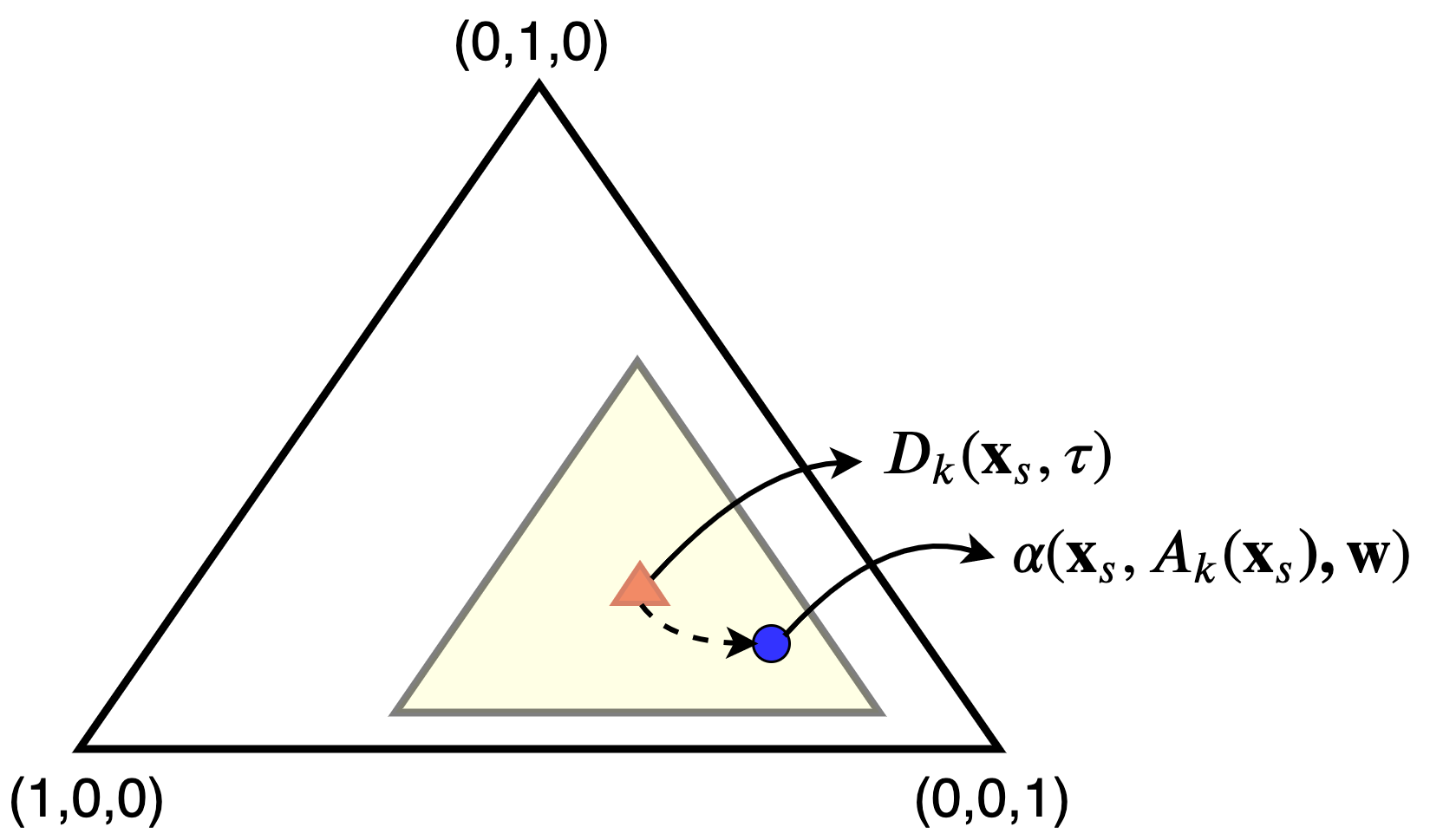
Let us consider the attention weights produced by the sum in detail. If is a point in the unit simplex, then belongs to a subsimplex whose size depends on the value of . The unit simplex for the case (three decision trees) with vertices , , is depicted in Fig. 1 where the small triangle and the small circle are points and , respectively. It can be seen from Fig. 1 that the attention weights are located in the subsimplex of a smaller size. The corresponding point is biased by the vector whose optimal value is computed by solving the quadratic optimization problem (15). The attention weight point cannot be outside the small subsimplex whose center is , and its size is defined by parameter . On the one hand, we should increase in order to increase the subsimplex and to extend the set of solutions. On the other hand, the extension of the solution set may lead to the sparse solution and to reducing the role of instances because weights of trees in this case are obtained mainly from , and they do not take into account relationship between and . The optimal choice of is carried out by testing ABRF-1 for different values of .
The first advantage of ABRF-1 modification is that it is simple from the computational point of view because its training is based on solving the standard quadratic optimization problem. The second advantage is that if is a probability distribution, then, due to the -contamination model the attention weights also compose a probability distribution. This implies that we do not need to worry about non-negative values of weights and the unit sum of weights. The third advantage of ABRF-1 is that it is simply interpreted, i.e., the obtained weights indicate which decision trees significantly contribute into the RF prediction.
4.1.2 A case of linear programming
So far, we have studied the case of -norm for defining the loss function in (11). This norm leads to the quadratic optimization problem in the ABRF-1 model. However, we can also consider the -norm. It turns out that this norm leads to the linear optimization problem. Denote for simplicity
| (17) |
Then we can rewrite optimization problem (15) by using the -norm as follows:
| (18) |
Introduce the following optimization variables:
| (19) |
Then we get the linear optimization problem:
| (20) |
subject to , , and ,
| (21) |
| (22) |
The above problem has variables and linear constraints. Its solution does not meet any difficulties.
4.2 ABRF-2
Another modification (ABRF-2) is based on using conventional definitions of the attention scoring function when trainable parameters are incorporated into the score function [13, 14, 1, 15]. One of the simplest way for defining the attention weights is to apply (3). Then we get the following weight for the -th tree:
| (23) |
where is the vector of training parameters such that ; is the training vector of the feature weights.
In fact, we replace the vector of parameters by the vector and the vector . It should be noted that the temperature parameter is no longer used because it is incorporated into training parameters . In this case, optimization problem (12) with (23) cannot be represented as the quadratic optimization problem. However, optimal values of parameters and can be found by means of well-known optimization methods, for example, by means of the gradient descent algorithm. It should be also noted that only one of the vectors and can be used as trainable parameters of the attention mechanism. However, our numerical experiments show that both vectors and provide outperforming results.
4.3 ABRF-3
The third modification (ABRF-3) combines ABRF-1 and ABRF-2 models, i.e., it uses three vectors of training parameters , and . Vectors and are incorporated into the softmax operation (see ABRF-2), vector forms the -contamination model. As a result, we get the optimization problem whose objective function coincides with (15), but it is minimized over unit simplices produced by vectors and . Weights of trees are defined now as follows:
| (24) |
Substituting the above expression into (11), we get the objective function of the optimization problem with obvious constraints:
| (25) |
| (26) |
The obtained optimization problem can be solved by means of the gradient descent algorithm.
5 Attention-based RF: Classification models
After studying the attention-based RF for regression, the similar machine learning problem can be formally stated for classification. In this case, the output represents the class of the associated instance. The task of classification is to construct an accurate classifier which can predict the unknown class label of a new observation , using available training data, such that it minimizes the classification expected risk.
An important property of decision trees is a probability distribution of classes determined at each leaf node. This probability distribution can be used for computing probabilities of classes for the whole RF and for making decision about a class label of a testing instance. Suppose that training instances fall into leaf node such that vectors belong to classes , respectively. Here there holds . Then the class probability distribution for example , which falls into leaf node , is , and it can be computed as , . Index of the leaf node in notations of is not used again because instance can fall only into one leaf.
Attention-based classification RF differs from the regression problem statement (see (8)-(11)) only by the class probability distributions instead of the point-valued target . If we again denote the tree attention weight as , then the class probability distribution of the whole RF can be written (see (8)-(11)) as follows:
| (27) |
Hence, the optimization problem for computing trainable vectors defining the tree attention weight is of the form:
| (28) |
where the loss function is defined as the expected distance between the one-hot vector and the RF class probability distribution, i.e., there holds
| (29) |
Here the one-hot vector has the unit element with the index corresponding to the class of the -th instance. Vector is determined from the training set whereas vector is computed after training decision trees counting instances from classes, which fall into the corresponding leaf node.
Objective function (15) can be rewritten for the classification case as follows:
| (30) |
where is computed in accordance with (16).
One can see from the above that modifications ABRF-1, ABRF-2, ABRF-3 for classification can be simply reduced to optimization problems which are similar to the same problems for regression.
6 Numerical experiments
6.1 Regression
In order to study the proposed approach for solving regression problems, we apply datasets which are taken from open sources, in particular: Diabetes can be found in the corresponding R Packages; Friedman 1, 2 3 are described at site: https://www.stat.berkeley.edu/~breiman/bagging.pdf; Regression and Sparse datasets are available in package “Scikit-Learn”. The proposed algorithm is evaluated and investigated also by the following publicly available datasets from the UCI Machine Learning Repository [33]: Wine Red, Boston Housing, Concrete, Yacht Hydrodynamics, Airfoil. A brief introduction about these data sets are given in Table 1 where and are numbers of features and instances, respectively. A more detailed information can be found from the aforementioned data resources.
| Data set | Abbreviation | ||
|---|---|---|---|
| Diabetes | Diabetes | ||
| Friedman 1 | Friedman 1 | ||
| Friedman 2 | Friedman 2 | ||
| Friedman 3 | Friedman 3 | ||
| Scikit-Learn Regression | Regression | ||
| Scikit-Learn Sparse Uncorrelated | Sparse | ||
| UCI Wine red | Wine | ||
| UCI Boston Housing | Boston | ||
| UCI Concrete | Concrete | ||
| UCI Yacht Hydrodynamics | Yacht | ||
| UCI Airfoil | Airfoil |
We use the coefficient of determination denoted and the mean absolute error (MAE) for the regression evaluation. The greater the value of the coefficient of determination and the smaller the MAE, the better results we get. In all tables, we compare and the MAE for three cases:
-
1.
RF: the RF or the ERT without the softmax and without attention model;
-
2.
Softmax model: the RF or the ERT with softmax operation without trainable parameters, i.e., weights of trees are determined in accordance with (16), and they are used to calculate the RF performance measures as the weighted sum of the tree outcomes.
-
3.
ABRF-1, ABRF-2, ABRF-3: one of the ABRF models.
The best results in all tables are shown in bold. Moreover, for cases of studying ABRF-1 and ABRF-3 models, the optimal values of the contamination parameter are provided. The case means that weights of trees are totally determined by the tree results and do not depend on each instance. This case coincides with the weighted RF proposed in [30]. The case means that weights of trees are determined only by the softmax function (with or without trainable parameters).
All experiments can be divided into two groups:
-
1.
The first group, called Condition 1, is based on training trees in RFs or ERTs such that the largest depth of trees is 2. This condition is used in order to ensure to have in each leaf more than one instance. At the same time, the restriction of the tree depth may cause a lower quality of trees.
-
2.
The second group, called Condition 2, is based on training trees such that at least instances fall into every leaf of trees. This condition is used to get desirable estimates of vectors .
Every RF or ERT consists of decision trees. To evaluate the average accuracy measures, we perform a cross-validation with repetitions, where in each run, we randomly select training data and testing data.
6.1.1 ABRF-1
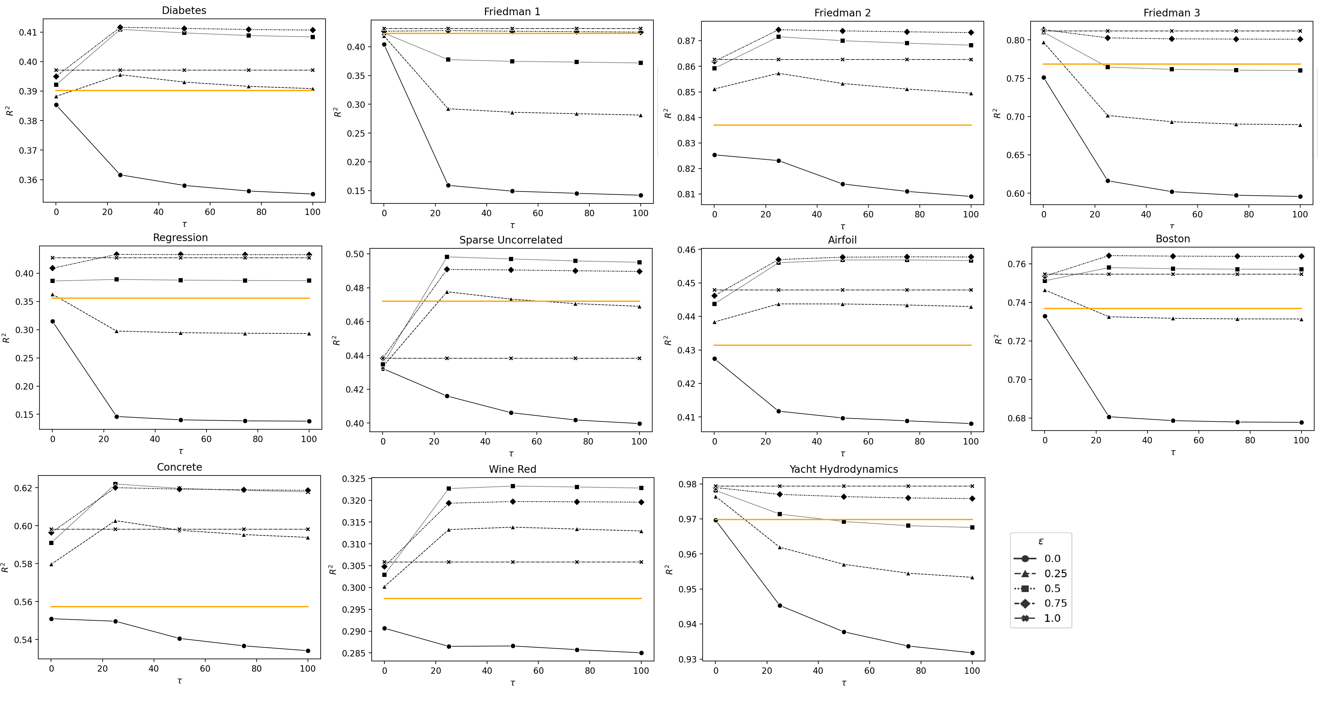
It should be noted that ABRF-1 has two tuning parameters and , which may significantly impact on predictions. Therefore, the best predictions are calculated at a predefined grid of the tuning parameters, and a cross-validation procedure is subsequently used to select an appropriate values of and . Fig. 2 demonstrates how parameters and impact on the performance measure () for all considered datasets under Condition 1. Each picture corresponding to a dataset in Fig. 2 shows measures as functions of for different values of such that each function corresponds to one value of . In particular, curves with circle, triangle, square, diamond, cross markers correspond to values , , , , of , respectively. The solid orange curve in each picture corresponds to when the original RF without attention-based model is used. The solid curve is depicted in order to illustrate the relationship between the original RF and ABRF-1 by different values of and . It can be seen from Fig. 2 that there is an optimal pair of values of and for each dataset, which provides the largest value of .
Measures and MAE for three cases (RF, Softmax and ABRF-1) are shown in Table 2. The results are obtained by training the RF and the parameter vector on the regression datasets under Condition 1 that the largest depth of trees is 2. It can be seen from Table 2 that ABRF-1 outperforms the RF and the Softmax models almost for all datasets. The same results are shown in Table 3 under Condition 2 that trees are built to ensure at least instances in each leaf. One can again see from Table 3 that ABRF-1 outperforms the RF and the Softmax models for most datasets.
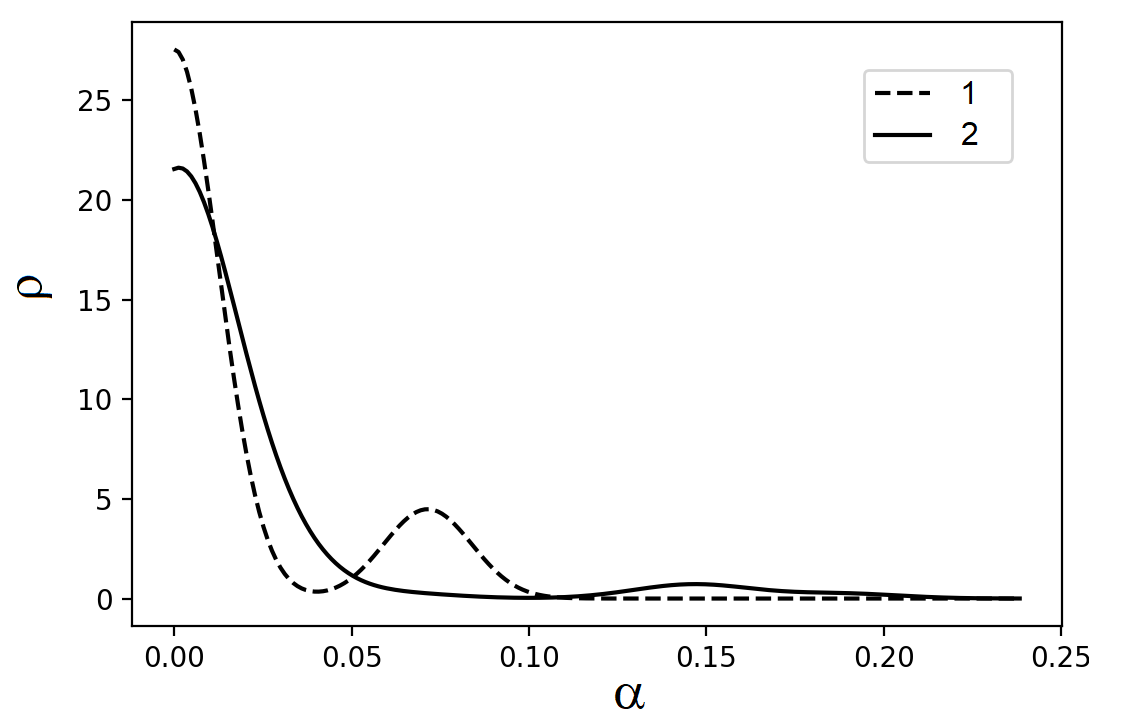
An example of two kernel density estimations (KDEs) as functions of the attention weight distributions over trees for a randomly selected instance is depicted in Fig. 3. The first KDE (the dash line 1) is constructed using the attention weights computed by means of the softmax operation without trainable parameters (the Softmax case). The second KDE (the solid line 2) is constructed using the ABRF-1 model. The Gaussian kernel with the unit variance is applied to constructing the KDEs. It can be seen from Fig. 3 that the attention weight distribution computed by using ABRF-1 differs from the first weight distribution. It can be regarded as a smooth version of the first distribution.
| MAE | |||||||
|---|---|---|---|---|---|---|---|
| Data set | RF | Softmax | ABRF-1 | RF | Softmax | ABRF-1 | |
| Diabetes | |||||||
| Friedman 1 | |||||||
| Friedman 2 | |||||||
| Friedman 3 | |||||||
| Regression | |||||||
| Sparse | |||||||
| Airfoil | |||||||
| Boston | |||||||
| Concrete | |||||||
| Wine | |||||||
| Yacht | |||||||
Another interesting question is how the attention-based model performs when ERTs are used. The corresponding results under Condition 1 and Condition 2 are shown in Tables 4 and 5, respectively. It is interesting to point out that ERTs provide comparable and even better results than RFs.
| MAE | |||||||
|---|---|---|---|---|---|---|---|
| Data set | ERT | Softmax | ABRF-1 | ERT | Softmax | ABRF-1 | |
| Diabetes | |||||||
| Friedman 1 | |||||||
| Friedman 2 | |||||||
| Friedman 3 | |||||||
| Regression | |||||||
| Sparse | |||||||
| Airfoil | |||||||
| Boston | |||||||
| Concrete | |||||||
| Wine | |||||||
| Yacht | |||||||
Performance measures of the linear modification of ABRF-1, when it is trained by using the linear optimization problem (20)-(22) under Condition 2 for the RF and for the ERT, are given in Tables 6 and 7, respectively. To compare the performance results obtained by means of the linear and quadratic optimization problems, we collect values of the measure for ABRF-1 from Table 6 and from Table 3 in Table 8. It can be seen from Table 8 that the quadratic optimization problem provides better results in comparison with the linear case. However, this outperformance is rather negligible. The same can be said if to compare the results under other conditions (ERTs and Condition 1).
| MAE | |||||||
|---|---|---|---|---|---|---|---|
| Data set | RF | Softmax | ABRF-1 | RF | Softmax | ABRF-1 | |
| Diabetes | |||||||
| Friedman 1 | |||||||
| Friedman 2 | |||||||
| Friedman 3 | |||||||
| Regression | |||||||
| Sparse | |||||||
| Airfoil | |||||||
| Boston | |||||||
| Concrete | |||||||
| Wine | |||||||
| Yacht | |||||||
| MAE | |||||||
|---|---|---|---|---|---|---|---|
| Data set | ERT | Softmax | ABRF-1 | ERT | Softmax | ABRF-1 | |
| Diabetes | |||||||
| Friedman 1 | |||||||
| Friedman 2 | |||||||
| Friedman 3 | |||||||
| Regression | |||||||
| Sparse | |||||||
| Airfoil | |||||||
| Boston | |||||||
| Concrete | |||||||
| Wine | |||||||
| Yacht | |||||||
| Data set | Linear | Quadratic |
|---|---|---|
| Diabetes | ||
| Friedman 1 | ||
| Friedman 2 | ||
| Friedman 3 | ||
| Regression | ||
| Sparse | ||
| Airfoil | ||
| Boston | ||
| Concrete | ||
| Wine | ||
| Yacht |
6.1.2 ABRF-2
Numerical experiments with ABRF-2 are presented in Tables 9-11. Since ABRF-2 is based only on the trainable softmax operation and does not use the contamination model, then we can take in all experiments with ABRF-2, and values of are not presented in tables with results. It can be seen from Tables 9-11 that ABRF-2 does not outperform the RF (the ERT) for many datasets. This implies that the attention-based model without the contamination component provides worse results in comparison with ABRF-1.
| MAE | ||||||
|---|---|---|---|---|---|---|
| Data set | RF | Softmax | ABRF-2 | RF | Softmax | ABRF-2 |
| Diabetes | ||||||
| Friedman 1 | ||||||
| Friedman 2 | ||||||
| Friedman 3 | ||||||
| Regression | ||||||
| Sparse | ||||||
| Airfoil | ||||||
| Boston | ||||||
| Concrete | ||||||
| Wine | ||||||
| Yacht | ||||||
| MAE | ||||||
|---|---|---|---|---|---|---|
| Data set | ERT | Softmax | ABRF-2 | ERT | Softmax | ABRF-2 |
| Diabetes | ||||||
| Friedman 1 | ||||||
| Friedman 2 | ||||||
| Friedman 3 | ||||||
| Regression | ||||||
| Sparse | ||||||
| Airfoil | ||||||
| Boston | ||||||
| Concrete | ||||||
| Wine | ||||||
| Yacht | ||||||
| MAE | ||||||
|---|---|---|---|---|---|---|
| Data set | RF | Softmax | ABRF-2 | RF | Softmax | ABRF-2 |
| Diabetes | ||||||
| Friedman 1 | ||||||
| Friedman 2 | ||||||
| Friedman 3 | ||||||
| Regression | ||||||
| Sparse | ||||||
| Airfoil | ||||||
| Boston | ||||||
| Concrete | ||||||
| Wine | ||||||
| Yacht | ||||||
6.1.3 ABRF-3
Numerical experiments with ABRF-2 are presented in Tables 12-14. One can see from the tables that ABRF-3 outperforms other models. In particular, as it is shown in Table 12, ABRF-3 provides better results for all datasets under Condition 1. In fact, this model clearly corrects inaccurate predictions of RFs trained under Condition 1. This is a very important property of ABRF-3. It should be noted that similar results were demonstrated by ABRF-1 when Condition 1 was used to train trees. However, it follows, for example, from Table 2, that there are a few datasets for which ABRF-1 provides worse results.
| MAE | |||||||
|---|---|---|---|---|---|---|---|
| Data set | RF | Softmax | ABRF-3 | RF | Softmax | ABRF-3 | |
| Diabetes | |||||||
| Friedman 1 | |||||||
| Friedman 2 | |||||||
| Friedman 3 | |||||||
| Regression | |||||||
| Sparse | |||||||
| Airfoil | |||||||
| Boston | |||||||
| Concrete | |||||||
| Wine | |||||||
| Yacht | |||||||
| MAE | |||||||
|---|---|---|---|---|---|---|---|
| Data set | ERT | Softmax | ABRF-3 | ERT | Softmax | ABRF-3 | |
| Diabetes | |||||||
| Friedman 1 | |||||||
| Friedman 2 | |||||||
| Friedman 3 | |||||||
| Regression | |||||||
| Sparse | |||||||
| Airfoil | |||||||
| Boston | |||||||
| Concrete | |||||||
| Wine | |||||||
| Yacht | |||||||
| MAE | |||||||
|---|---|---|---|---|---|---|---|
| Data set | RF | Softmax | ABRF-3 | RF | Softmax | ABRF-3 | |
| Diabetes | |||||||
| Friedman 1 | |||||||
| Friedman 2 | |||||||
| Friedman 3 | |||||||
| Regression | |||||||
| Sparse | |||||||
| Airfoil | |||||||
| Boston | |||||||
| Concrete | |||||||
| Wine | |||||||
| Yacht | |||||||
In Table 15, we compare all proposed attention-based models (ABRF-1, ABRF-2, ABRF-3) by using the measure and the same conditions (RFs built to ensure at least instances in every leaf). It can be seen from Table 15 that ABRF-3 is comparable with ABRF-1, but both the models outperform ABRF-2.
| Data set | ABRF-1 | ABRF-2 | ABRF-3 |
|---|---|---|---|
| Diabetes | |||
| Friedman 1 | |||
| Friedman 2 | |||
| Friedman 3 | |||
| Regression | |||
| Sparse | |||
| Airfoil | |||
| Boston | |||
| Concrete | |||
| Wine | |||
| Yacht |
6.2 Classification
To study the proposed attention-based models for solving classification problems, we apply datasets which are taken from the UCI Machine Learning Repository [33], in particular, Diabetic Retinopathy, Eeg Eyes, Haberman’s Survival, Ionosphere, Seeds, Seismic-Bumps, Soybean, Teaching Assistant Evaluation, Tic-Tac-Toe Endgame, Website Phishing, Wholesale Customer. Table 16 shows the number of features for the corresponding data set, the number of instances , the number of classes and their abbreviation. More detailed information can be found from the data resources.
score is used in the classification experiments as an accuracy measure which takes into account the class imbalance. Every RF consists of decision trees. To evaluate the average accuracy measures, we again perform a cross-validation with repetitions, where in each run, we randomly select training data and testing data.
| Data set | Abbreviation | |||
|---|---|---|---|---|
| Diabetic Retinopathy | Diabet | |||
| Eeg Eyes | Eeg | |||
| Haberman’s Survival | Haberman | |||
| Ionosphere | Ionosphere | |||
| Seeds | Seeds | |||
| Seismic-Bumps | Seismic | |||
| Soybean | Soybean | |||
| Teaching Assistant Evaluation | TAE | |||
| Tic-Tac-Toe Endgame | TTTE | |||
| Website Phishing | Phishing | |||
| Wholesale Customer | Wholesale |
Table 17 illustrates results of numerical experiments in the form of the measure with ABRF-1 solving the classification problem. Table 17 is similar to Tables 3-4 obtained for the regression problem. It can be seen from Table 17 that ABRF-1 mainly shows outperforming results. However, there are several datasets (Eeg, Ionosphere, Phishing) which demonstrate worse results for ABRF-1. This may be due to use of the Euclidean distance between the one-hot vector and the class probability distribution in the loss function (29). It is well-known that this comparison of the probability distributions is not the best way in classification. However, different distances between probability distributions, for example, the Kullback-Leibler divergence, complicates the optimization problem (30), which becomes non-quadratic. Therefore, the Euclidean distance is used to save properties of the ABRF-1 simplicity.
| Condition 1 | Condition 2 | |||||||
|---|---|---|---|---|---|---|---|---|
| Data set | RF | Softmax | ABRF-1 | RF | Softmax | ABRF-1 | ||
| Diabet | ||||||||
| Eeg | ||||||||
| Haberman | ||||||||
| Ionosphere | ||||||||
| Seeds | ||||||||
| Seismic | ||||||||
| Soybean | ||||||||
| TAE | ||||||||
| TTTE | ||||||||
| Phishing | ||||||||
| Wholesale | ||||||||
Table 18 shows the measures obtained for ABRF-2 and ABRF-3 under Condition 2. We do not show results corresponding to Condition 1 because they are similar to results presented for Condition 2. Values of are shown in Table 18 for the ABRF-3 model. One can see from Table 18 that the results correlate with the same results for regression (see Tables (9)-(11)), i.e., the ABRF-2 model does not show any sufficient improvement in comparison with the original RF. In contrast to results presented in Table 18 for ABRF-2 and even in Table 17 for ABRF-1, the ABRF-3 model provides outperforming results as it is shown in Table 18. However, it is interesting to point out that ABRF-3 is actually reduced to ABRF-1 for several datasets when . In this case, the term with the softmax function is not used, and the attention weights are entirely determined by the -contamination model. United results obtained for the case of the ERT usage under Condition 2 are presented in Table 19. It can be again seen from Table 19 that the proposed attention-based models outperform the ERT and the ERT with the softmax function without its training for all considered datasets.
In sum, results of numerical experiments for classification generally coincide with the results obtained for regression. Analyzing these results, we can conclude that the ABRF-3 is comparable with ABRF-1 for regression as well as for classification. Moreover, numerical experiments show that ABRF-3 provides results which are slightly better than results of ABRF-1. However, ABRF-1 is computationally much more simpler than the ABRF-3 model because it is based on solving the linear or quadratic optimization problems whereas ABRF-3 requires to solve the complex optimization problems for training.
| Data set | RF | Softmax | ABRF-2 | ABRF-3 | |
|---|---|---|---|---|---|
| Diabet | |||||
| Eeg | |||||
| Haberman | |||||
| Ionosphere | |||||
| Seeds | |||||
| Seismic | |||||
| Soybean | |||||
| TAE | |||||
| TTTE | |||||
| Phishing | |||||
| Wholesale |
| Data set | ERT | Softmax | ABRF-1 | ABRF-2 | ABRF-3 |
|---|---|---|---|---|---|
| Diabet | |||||
| Eeg | |||||
| Haberman | |||||
| Ionosphere | |||||
| Seeds | |||||
| Seismic | |||||
| Soybean | |||||
| TAE | |||||
| TTTE | |||||
| Phishing | |||||
| Wholesale |
7 Concluding and discussion remark
New models of the attention-based RF have been proposed. They inherit the best properties of the attention mechanism and allow us to avoid using neural networks. Moreover, some models allow us to avoid using the gradient-based algorithms for computing the trainable parameters of the attention because the quadratic or linear programming can be applied to training. The idea to avoid differentiable nonlinear modules in machine learning models has been highlighted by Zhou and Feng [34] where it has been realized in the so-called deep forests. We also tried to realize this idea in the attention mechanism by applying it to RFs and by introducing the Huber’s -contamination model in ABRF-1. At the same time, we did not deny applying the gradient-based algorithm as an efficient tool for solving optimization problems, and ABRF-2, ABRF-3 have also demonstrated desirable results. However, they tend to overfitting for some datasets and parameters. Therefore, we think that the most interesting model is ABRF-1.
Let us point out advantages of the proposed models. First, the ABRF-1 models are simply trained by solving the standard quadratic or linear optimization problems. Second, the proposed usage of the Huber’s -contamination model extends the set of weight functions in attention models. Third, the proposed models are flexible and can be simply modified. For example, different procedures for computing values can be proposed and studied, different kernels can be used instead of the softmax. Fourth, the attention-based approach allows us to significantly improve predictions, and numerical experiments have illustrated this improvement on several datasets. Fifth, the results are interpretable because the attention weights show which decision trees have the largest contribution into predictions. Sixth, when new training instances appear after building the RF, we do not need to rebuild trees because it is enough to train weights of trees. Finally, the models are implementation of the attention mechanism on RFs without neural networks.
The following disadvantages should be also pointed out. First, the RF is not the best classifier or regressor. It perfectly deals with tabular data, but many other types of data, for example, images, may result unsatisfactory predictions in comparison with, for example, neural networks. Second, the ABRF-1 model is very simple from the computation point of view. However, it has the tuning parameter which requires to solve many optimization problems in order to get the best results. Moreover, we have to take into account the temperature parameter of the softmax function. Third, most attention models directly provide weights of instances. The proposed ABRF models compute weights of trees. It should be noted that the weights of instances can be calculated through the weights of trees, but an additional analysis has to be performed for doing that.
Numerical experiments have demonstrated that the attention models can significantly improve original RFs. Moreover, many extensions and new models can be developed due to flexibility of the ABRF models. First of all, it is interesting to extend the proposed approach to the gradient boosting machine [35] which is based on decision trees as week learners. It is also interesting to extend the approach on deep forests [34]. These are directions for further research. Another interesting direction for research is to investigate various functions instead of the softmax which is used in the proposed models. It is obvious that kernel functions should be used. Choice of the kernel functions, which lead to simple computations and outperforming prediction results, is a direction for further research. In models ABRF-1 and ABRF-3, objective functions have been optimized over the whole set of weights, i.e., over the unit simplex. However, the set of weights can be restricted under various conditions. This restriction may prevent from overfitting. Moreover, there are other statistical contamination models [36] which could be incorporated into the ABRF models. These ideas can be also viewed as directions for further research. Finally, we have considered the distance between vectors and inside one leaf where the instance falls into. However, it may be useful to extend this distance definition and to study some weighted sum of distances between and vectors which are defined for nearest neighbor leaves. Moreover, there are different definitions of vector itself, for example, we can use the median instead of the mean value. This is also an interesting direction for further research.
Acknowledgement
This work is supported by the Russian Science Foundation under grant 21-11-00116.
References
- [1] Z. Niu, G. Zhong, and H. Yu. A review on the attention mechanism of deep learning. Neurocomputing, 452:48–62, 2021.
- [2] S. Chaudhari, V. Mithal, G. Polatkan, and R. Ramanath. An attentive survey of attention models. arXiv:1904.02874, Apr 2019.
- [3] A.S. Correia and E.L. Colombini. Attention, please! A survey of neural attention models in deep learning. arXiv:2103.16775, Mar 2021.
- [4] A.S. Correia and E.L. Colombini. Neural attention models in deep learning: Survey and taxonomy. arXiv:2112.05909, Dec 2021.
- [5] T. Lin, Y. Wang, X. Liu, and X. Qiu. A survey of transformers. arXiv:2106.04554, Jul 2021.
- [6] L. Breiman. Random forests. Machine learning, 45(1):5–32, 2001.
- [7] L.V. Utkin, M.S. Kovalev M.S., and F. Coolen. Imprecise weighted extensions of random forests for classification and regression. Applied Soft Computing, 92(Article 106324):1–14, 2020.
- [8] L.V. Utkin, M.S. Kovalev, and A.A. Meldo. A deep forest classifier with weights of class probability distribution subsets. Knowledge-Based Systems, 173:15–27, 2019.
- [9] A. Zhang, Z.C. Lipton, M. Li, and A.J. Smola. Dive into deep learning. arXiv:2106.11342, Jun 2021.
- [10] E.A. Nadaraya. On estimating regression. Theory of Probability & Its Applications, 9(1):141–142, 1964.
- [11] G.S. Watson. Smooth regression analysis. Sankhya: The Indian Journal of Statistics, Series A, pages 359–372, 1964.
- [12] P.J. Huber. Robust Statistics. Wiley, New York, 1981.
- [13] D. Bahdanau, K. Cho, and Y. Bengio. Neural machine translation by jointly learning to align and translate. arXiv:1409.0473, Sep 2014.
- [14] T. Luong, H. Pham, and C.D. Manning. Effective approaches to attention-based neural machine translation. In Proceedings of the 2015 Conference on Empirical Methods in Natural Language Processing, pages 1412–1421. The Association for Computational Linguistics, 2015.
- [15] A. Vaswani, N. Shazeer, N. Parmar, J. Uszkoreit, L. Jones, A.N. Gomez, L. Kaiser, and I. Polosukhin. Attention is all you need. In Advances in neural information processing systems, pages 5998–6008, 2017, 2017.
- [16] P. Geurts, D. Ernst, and L. Wehenkel. Extremely randomized trees. Machine learning, 63:3–42, 2006.
- [17] F. Liu, X. Huang, Y. Chen, and J.A. Suykens. Random features for kernel approximation: A survey on algorithms, theory, and beyond. arXiv:2004.11154v5, Jul 2021.
- [18] K. Choromanski, V. Likhosherstov, D. Dohan, X. Song, A. Gane, T. Sarlos, P. Hawkins, J. Davis, A. Mohiuddin, L. Kaiser, D. Belanger, L. Colwell, and A. Weller. Rethinking attention with performers. In 2021 International Conference on Learning Representations, 2021.
- [19] X. Ma, X. Kong, S. Wang, C. Zhou, J. May, H. Ma, and L. Zettlemoyer. Luna: Linear unified nested attention. arXiv:2106.01540, Nov 2021.
- [20] K. Choromanski, H. Chen, H. Lin, Y. Ma, A. Sehanobish, D. Jain, M.S. Ryoo, J. Varley, A. Zeng, V. Likhosherstov, D. Kalachnikov, V. Sindhwani, and A. Weller. Hybrid random features. arXiv:2110.04367v2, Oct 2021.
- [21] H. Peng, N. Pappas, D. Yogatama, R. Schwartz, N. Smith, and L. Kong. Random feature attention. In International Conference on Learning Representations (ICLR 2021), pages 1–19, 2021.
- [22] I. Schlag, K. Irie, and J. Schmidhuber. Linear transformers are secretly fast weight programmers. In International Conference on Machine Learning 2021, pages 9355–9366. PMLR, 2021.
- [23] H. Kim, H. Kim, H. Moon, and H. Ahn. A weight-adjusted voting algorithm for ensemble of classifiers. Journal of the Korean Statistical Society, 40(4):437–449, 2011.
- [24] H. B. Li, W. Wang, H. W. Ding, and J. Dong. Trees weighting random forest method for classifying high-dimensional noisy data. In 2010 IEEE 7th International Conference on E-Business Engineering, pages 160–163. IEEE, Nov 2010.
- [25] C.A. Ronao and S.-B. Cho. Random forests with weighted voting for anomalous query access detection in relational databases. In Artificial Intelligence and Soft Computing. ICAISC 2015, volume 9120 of Lecture Notes in Computer Science, pages 36–48, Cham, 2015. Springer.
- [26] S.J. Winham, R.R. Freimuth, and J.M. Biernacka. A weighted random forests approach to improve predictive performance. Statistical Analysis and Data Mining, 6(6):496–505, 2013.
- [27] S. Xuan, G. Liu, and Z. Li. Refined weighted random forest and its application to credit card fraud detection. In Computational Data and Social Networks, pages 343–355, Cham, 2018. Springer International Publishing.
- [28] X. Zhang and M. Wang. Weighted random forest algorithm based on bayesian algorithm. In Journal of Physics: Conference Series, volume 1924, pages 1–6. IOP Publishing, 2021.
- [29] M.E.H. Daho, N. Settouti, M.E.A. Lazouni, and M.E.A. Chikh. Weighted vote for trees aggregation in random forest. In 2014 International Conference on Multimedia Computing and Systems (ICMCS), pages 438–443. IEEE, April 2014.
- [30] L.V. Utkin, A.V. Konstantinov, V.S. Chukanov, and A.A. Meldo. A new adaptive weighted deep forest and its modifications. International Journal of Information Technology & Decision Making, 19(4):963–986, 2020.
- [31] L.V. Utkin, A.V. Konstantinov, V.S. Chuknov, M.V. Kots, M.A. Ryabinin, and A.A. Meldo. A weighted random survival forest. arXiv:1901.00213, Jan 2019.
- [32] J.O. Berger. Statistical Decision Theory and Bayesian Analysis. Springer-Verlag, New York, 1985.
- [33] D. Dua and C. Graff. UCI machine learning repository, 2017.
- [34] Z.-H. Zhou and J. Feng. Deep forest. National Science Review, 6(1), 2019.
- [35] J.H. Friedman. Stochastic gradient boosting. Computational statistics & data analysis, 38(4):367–378, 2002.
- [36] P. Walley. Statistical Reasoning with Imprecise Probabilities. Chapman and Hall, London, 1991.