Decoupling Makes Weakly Supervised Local Feature Better

Abstract

Weakly supervised learning can help local feature methods to overcome the obstacle of acquiring a large-scale dataset with densely labeled correspondences. However, since weak supervision cannot distinguish the losses caused by the detection and description steps, directly conducting weakly supervised learning within a joint training describe-then-detect pipeline suffers limited performance. In this paper, we propose a decoupled training describe-then-detect pipeline tailored for weakly supervised local feature learning. Within our pipeline, the detection step is decoupled from the description step and postponed until discriminative and robust descriptors are learned. In addition, we introduce a line-to-window search strategy to explicitly use the camera pose information for better descriptor learning. Extensive experiments show that our method, namely PoSFeat (Camera Pose Supervised Feature), outperforms previous fully and weakly supervised methods and achieves state-of-the-art performance on a wide range of downstream task.

1 Introduction

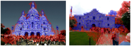
(a)

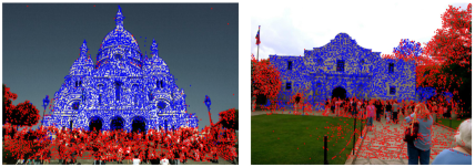
(b)

Figure 1: An illustration of the influence of ambiguity for weakly supervised local feature methods. Keypoints that succeed and fail to create landmarks are shown. (a) With joint training describe-then-detect pipeline, DISK-W [46] produces inaccurate keypoints that are out of the objects. (b) With our decoupled training describe-then-detect pipeline, PoSFeat can produce more reasonable keypoints. Best viewed in color.

Finding pixel correspondences is a fundamental problem in computer vision. Sparse local feature [22, 5, 36, 12, 48], as one of the mainstream methods to find correspondences, has been widely applied in many areas, such as simultaneous localization and mapping (SLAM) [29, 52], structure from motion (SfM) [40, 1], and visual localization [38, 7, 51, 16].

Traditional sparse local feature methods [22, 5, 36] follow a detect-then-describe pipeline. Specifically, keypoints are first detected and then patches centered at these keypoints are used to generate descriptors. Early methods [15, 17, 22, 19] focus on the detection step and are proposed to distinguish distinctive areas to detect good keypoints. Later works pay more attention to the description step and make attempts to design powerful descriptors using advanced representations [5, 8, 36].

Motivated by the success of deep learning, many efforts [50, 27, 31, 23, 44] have been made to replace the detection or description step in the detect-then-describe pipeline with CNNs. Recent works [13, 34, 24, 46] find that keypoints and descriptors are interdependent and propose a joint training describe-then-detect pipeline. Specifically, the description network and detection network are combined into a single CNN and optimized jointly. The joint training describe-then-detect pipeline achieves better performance than the detect-then-describe pipeline, especially under challenging conditions [45, 18]. However, these methods are fully supervised and rely on dense ground-truth correspondence labels for training.

Because collecting a large dataset with pixel-level ground-truth correspondences is expensive, self-supervised and weakly supervised learning are investigated for training. Specifically, DeTone et al. [12] used a single image and a virtual homography to generate image pairs to conduct self-supervised learning. However, homography transformation cannot cover complicated geometry transformations in real-world settings, resulting in limited performance. Noh et al. [30] used landmark labels to train the local feature network, which suffers extremely poor performance on viewpoint changes. Owing to the convenience of collecting camera poses, Wang et al. [47] introduced camera poses as weak supervision for descriptor learning. Although weakly supervised learning achieves promising results within the detect-then-describe pipeline, directly applying it to the joint training describe-then-detect pipeline is hard to produce satisfying results [46].

When a detection network and a description network are jointly optimized within a joint training describe-then-detect pipeline with only weak supervision (e.g., camera pose), the loss produced by these two components cannot be distinguished. Specifically, when only one component is failed (Fig. 2), both the detection network and the description network cannot be correctly updated within a joint training describe-then-detect pipeline. As a result, the description network is hard to produce highly discriminative descriptors, and the detection network may produce false detected keypoints that are out of object boundaries, as shown in Fig. 1.

In this paper, we propose a decoupled training describe-then-detect pipeline tailored for weakly supervised local feature learning. Our main insight is that, with only weak supervision, the detection network relies heavily on a good descriptor for accurate keypoint detection (Fig. 1). Consequently, we decouple the detection network from the description network to postpone it until a discriminative and robust descriptor is learned. Different from the detect-then-describe pipeline that relies on low-level structures for early detection, our keypoints detection depends on the higher-level structures encoded in the descriptors. As a result, better robustness is achieved. In contrast to the joint training describe-then-detect pipeline that simultaneously perform detection and description optimization, the two networks are trained separately and thus the loss function for these two components are decoupled to address the ambiguity. It is demonstrated that our decoupled training describe-then-detect pipeline facilitates local feature methods to achieve much better performance with only weak supervision. Our contributions can be summarized as:

(1) We introduce a decoupled training describe-then-detect pipeline for weakly supervised local feature learning. This simple yet efficient pipeline significantly improves the performance of weakly supervised local features.

(2) We propose a line-to-window search strategy to exploit the weak supervision of camera poses for descriptor learning. This strategy can make full use of the geometric information of camera poses to reduce the search space and learn highly discriminative descriptors.

(3) Our method achieves state-of-the-art performance on three datasets and largely closes the gap between fully and weakly supervised methods.

Figure 2: Motivation of decoupling. Two reasonable keypoints can be matched incorrectly due to the low discriminativeness of descriptors (e.g., caused by repetitive textures). Meanwhile, two false detected keypoints can also be matched with a high descriptor similarity. Best viewed in color.

2 Related Works

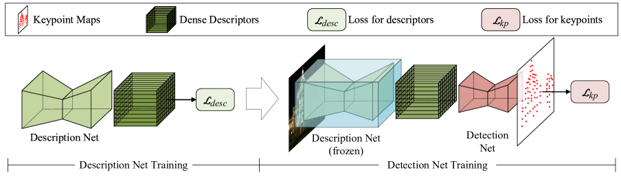
Figure 3: The proposed decoupled training describe-then-detect pipeline. The detection network is decoupled from the description network and postponed until good descriptors are obtained.

2.1 Fully Supervised Local Feature Methods

Fully supervised methods conduct local feature learning using pixel-level ground-truth correspondences to provide supervision. Following the detect-then-describe pipeline, early learning-based methods [39, 4, 27, 44, 14, 23] use CNNs to perform the detection or description steps. Specifically, QuadNet [39] and Key.Net [4] were proposed to use CNNs for keypoint detection. HardNet [27] and SOSNet [44] were developed to leverage CNNs to extract descriptors. Later, LIFT [50] and LFNet [31] were introduced to integrate both detection and description steps into an end-to-end architecture to achieve better performance. Note that, LIFT [50] also introduced a decoupled training to address unstable training issue with full supervision in a detect-then-describe pipeline.

Recent works [13, 34, 24, 46] follow a joint training describe-then-detect pipeline in which detection and description are combined into a single CNN and optimized jointly. Specifically, Dusmanu et al. [13] first used a CNN to extract dense features and then selected local maxima of the dense feature map as keypoints. Revaud et al. [34] further took both the repeatablity and reliability of the descriptors into consideration for better keypoint detection. Tyszkiewicz et al. [46] used policy gradient to address the discreteness during the selection of sparse keypoints (namely, DISK). Luo et al. [24] adopted deformable convolution to model the geometry information and detected keypoints at multiple scales. By jointly optimizing the detection network and the description network, joint training describe-then-detect pipeline achieves better performance than previous detect-then-describe pipeline.

2.2 Self-Supervised Local Feature Methods

As a large dataset with densely labeled correspondences is difficult to collect, self-supervised learning has been studied for local feature learning. Specifically, DeTone et al. [12] used a virtual homography to generate an image pair from a single image to conduct self-supervised learning. This method uses a CNN pretrained on synthetic data as a teacher of the detection network. Differently, Christiansen et al. [11] proposed an end-to-end framework to train both the detection network and the description network using virtual homography in a self-supervised manner. Later, Parihar et al. [32] leveraged the homography to enhance the robustness of descriptors to rotation. Nevertheless, simple homography transformations used in these self-supervised methods may not hold in real cases.

2.3 Weakly Supervised Local Feature Methods

Noh et al. introduced DELF [30], which is trained with an image retrieval task, to achieve local feature extraction. However, the keypoints detected by DELF are sensitive to vierwpoint changew and thus cannot be applied in real world settings. For camera poses are easy to collect, Wang et al. [47] used them as weak supervision and introduced an epipolar loss for descriptor learning. This method follows a detect-then-describe pipeline and relies on an off-the-shelf detection method (e.g., SIFT) to detect keypoints. Recently, Tyszkiewicz et al. [46] developed DISK-W to integrate weakly supervised learning in a joint training describe-then-detect pipeline by adopting policy gradient. Nevertheless, when DISK-W is directly trained with a weakly supervised loss (rather than a fully-supervised loss), it suffers a notable performance drop on pixel-wise metrics. As weakly supervised loss cannot distinguish between errors introduced by false keypoints and inaccurate descriptors, this ambiguity hinders the joint training describe-then-detect pipeline to learn good local features.

2.4 Learning-based Matcher Methods

Since a Brute Force Matcher (also named NN matcher) usually produces low quality raw matches, learning-based matchers are proposed to achieve better matching results. Sarlin et al. [37] proposed SuperGlue to achieve robust matching with a graph neural network (GNN) and an optimal transport algorithm. Chen et al. [10] improved the architecture of GNN to increase the efficiency of descriptor enhancement. Zhou et al. [53] proposed a weakly supervised network to refine raw matches using patch matches as prior. Sun et al. [42] introduced a detector-free matcher to achieve pixel correspondence in a coarse-to-fine manner. Note that, most matcher methods are not the direct competitors of local feature methods. Instead, they can be considered as a post processing step and combined with local features to achieve improved performance.

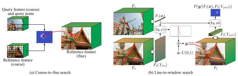
Figure 4: An illustration of the coarse-to-fine search strategy (a) and our line-to-window search strategy (b). The red line in $F_{2}$ denotes the epipolar line corresponding to the query point in $F_{1}$.

3 Decoupled Training Describe-then-Detect Pipeline

3.1 Overview

The decoupled training describe-then-detect pipeline is shown in Fig. 3. We train the description net and detection net individually to suppress the loss ambiguity caused by weak supervision. During training, we first leave out the detection network and optimize the description network to learn good descriptors with a line-to-window strategy. The description network is then frozen to train a detection network for keypoint detection. We follow CAPS [47] to use ResUNet as the description net, which produces a feature map with 1/4 resolution and 128 dimensions as dense descriptors. Additionally, we design a shallow detection net to detect keypoints at the original resolution. For more details about the network architecture, please refer to the supplementary material.

3.2 Feature Description

Following the widely used paradigm [47], we impose supervision only on sparse query points sampled from paired images to conduct training of the description network. We first split an image into small grids of size $g_{d}\times g_{d}$, and randomly sample one point per grid as a query point. Then, we translate relative camera pose into an epipolar constraint and introduce a line-to-window search strategy to reduce search space (Sec. 3.2.1). Moreover, we formulate a loss function by encouraging the predicted matches to obey the epipolar constraint (Sec. 3.2.2).

3.2.1 Line-to-Window Search

Given a query point $\boldsymbol{x}$ in the query image $I_{1}$, our goal is to find its correspondence in the reference image $I_{2}$. Since repetitive structures widely exist in a natural image, the commonly used coarse-to-fine strategy [47, 42] usually selects a mismatched patch such that inferior performance is produced (Fig. 4(a)). Intuitively, the correspondence of the query point $\boldsymbol{x}$ is constrained in an epipolar line in the reference image. Therefore, we introduce a line-to-window search strategy to reduce search space for better performance. Our line-to-window search strategy consists of two search steps, as illustrated in Fig. 4(b).

Search along An Epipolar Line.

For a query point $\boldsymbol{x}_{i}\in I_{1}$, we first calculate its corresponding epipolar line $L_{\boldsymbol{x}_{i}}$ in the reference image $I_{2}$ based on the relative camera pose. Then, we uniformly sample $N_{line}$ points along this epipolar line to formulate the search space $Y_{line}=\{\boldsymbol{y}_{i}^{j}\}(j=1,...,N_{line})$. Next, we calculate the matching probability of $\boldsymbol{x}_{i}$ over $Y_{line}$:

$$P({\boldsymbol{y}_{i}^{j}}|F_{1}({\boldsymbol{x}_{i}}),F_{2}(Y_{line}))=\frac{\exp(F_{1}({\boldsymbol{x}_{i}})^{\rm T}F_{2}({\boldsymbol{y}_{i}^{j}}))}{\sum_{Y_{line}}\exp(F_{1}({\boldsymbol{x}_{i}})^{\rm T}F_{2}({\boldsymbol{y}_{i}^{k}}))},$$ (1)

where $F_{1}$ and $F_{2}$ are the feature maps for $I_{1}$ and $I_{2}$, respectively. Afterwards, we select $\overline{\boldsymbol{y}}_{i}$ with the maximum probability from $Y_{line}$ to determine the coarse location of the correspondence of $\boldsymbol{x}_{i}$:

$$\overline{\boldsymbol{y}}_{i}=\mathop{\arg\max}\limits_{{\boldsymbol{y}_{i}^{j}}}P({\boldsymbol{y}_{i}^{j}}|F_{1}({\boldsymbol{x}_{i}}),F_{2}(Y_{line})).$$ (2)

Search in A Local Window.

Due to the discreteness of the candidates in $Y_{line}$, the resultant corresponding point $\overline{\boldsymbol{y}}_{i}$ can be far from the groundtruth. To remedy this, a subsequent search is conducted in a local window. First, we calculate the center of the local window:

$$\boldsymbol{y}_{i}^{center}=\overline{\boldsymbol{y}}_{i}+0.5\cdot w_{patch}\cdot\boldsymbol{u},$$ (3)

where $w_{patch}$ is the window size of a local patch, $\boldsymbol{u}\in\mathbb{R}^{2}$ is a noise vector drawn from a uniform distribution ${\rm U}(0,1)$ to avoid the convergence to trivial solution $F(\boldsymbol{x})\equiv{0}$. Then, a local patch $Y_{patch}\subset I_{2}$ centered at $\boldsymbol{y}_{i}^{center}$ is cropped from $F_{2}$ as the search space. Next, we calculate the matching probability of $\boldsymbol{x}_{i}$ over $Y_{patch}$:

$$P({\boldsymbol{y}_{i}^{j}}|F_{1}({\boldsymbol{x}_{i}}),F_{2}(Y_{patch}))=\frac{\exp(F_{1}({\boldsymbol{x}_{i}})^{\rm T}F_{2}({\boldsymbol{y}_{i}^{j}}))}{\sum_{Y_{patch}}\exp(F_{1}({\boldsymbol{x}_{i}})^{\rm T}F_{2}({\boldsymbol{y}_{i}^{k}}))}.$$ (4)

Because directly selecting the point with the maximum probability in the local patch is non-differentiable, we calculate the correspondence $\hat{\boldsymbol{y}}_{i}$ in a differentiable manner:

$$\hat{\boldsymbol{y}}_{i}=E({\boldsymbol{y}_{i}^{j}})=\sum_{{\boldsymbol{y}_{i}^{j}}\in Y_{patch}}{\boldsymbol{y}_{i}^{j}}\cdot P({\boldsymbol{y}_{i}^{j}}|F_{1}({\boldsymbol{x}_{i}}),F_{2}(Y_{patch})).$$ (5)

Compared to the previous coarse-to-fine search strategy [47], our line-to-window search strategy can make better use of the camera pose information to reduce search space and further improve the discriminativeness of descriptors (as demonstrated in Sec. 4.3).

3.2.2 Loss Function

With only weak supervision of camera pose, we calculate the distance of the correspondence $\hat{\boldsymbol{y}}_{i}$ to the epipolar line $L_{\boldsymbol{x}_{i}}$ as the loss of query point $\boldsymbol{x}_{i}$ [47]:

$$\mathcal{L}_{epi}({\hat{\boldsymbol{y}}_{i}},\boldsymbol{x}_{i})={\rm distance}({\hat{\boldsymbol{y}}_{i}},~{}{L_{\boldsymbol{x}_{i}}}).$$ (6)

Then, we use the weighted sum of the losses over all query points as the final loss:

$$\mathcal{L}_{desc}=\frac{\sum_{i}\frac{M_{i}}{{\sigma}(\boldsymbol{x}_{i})}\cdot\mathcal{L}_{epi}(\hat{\boldsymbol{y}}_{i},{\boldsymbol{x}_{i}})}{\sum_{i}\frac{M_{i}}{{\sigma}(\boldsymbol{x}_{i})}}.$$ (7)

Here, $M_{i}$ is a binary mask (which is used to exclude query points whose epipolar lines are not in the reference image) and ${\sigma}(\boldsymbol{x}_{i})$ is the variance of the probability distribution over $Y_{patch}$,

$${\sigma}(\boldsymbol{x}_{i})=\lVert\hat{\boldsymbol{y}}_{i}^{2}-E({\boldsymbol{y}_{i}^{j2}})\rVert$$ (8)

3.3 Feature Detection

After feature description learning, the description network is frozen to produce dense descriptors for keypoint detection, as shown in Fig. 3. Since selecting discrete sparse keypoints is non-differentiable, we adopt the strategy introduced in DISK [46], which is based on policy gradient, to achieve network training.

First, dense descriptors $F_{1}$ and $F_{2}$ are respectively extracted from $I_{1}$ and $I_{2}$, and fed to a detection network to produce keypoint heatmaps. Then, we divide these heatmaps into grids of size $g_{k}\times g_{k}$ and select at most one keypoint from each grid cell. Specifically, we establish a probability distribution $P_{kp}$ over each grid cell based on the heatmap scores in this cell. Afterwards, $P_{kp}$ is used to probabilistically select candidate keypoints $Q_{1}\!=\!\{{\boldsymbol{x}_{1}},{\boldsymbol{x}_{2}},\cdots\}$ and $Q_{2}\!=\!\{{\boldsymbol{y}_{1}},{\boldsymbol{y}_{2}},\cdots\}$ from $I_{1}$ and $I_{2}$, respectively. Next, a matching probability $P_{m}$ is calculated based on the feature similarity $S_{i,j}$ between each pair of candidate keypoints $(\boldsymbol{x}_{i},\boldsymbol{y}_{j})$. With only camera pose supervision, we adopt an epipolar reward similar to Eq. 6 to encourage $\boldsymbol{y}_{j}$ to be close to the epipolar line of $\boldsymbol{x}_{i}$ (i.e., $L_{\boldsymbol{x}_{i}}$):

$$R(\boldsymbol{x}_{i},\boldsymbol{y}_{j})=\begin{cases}\lambda_{p},&\mbox{if }{\rm distance}(\boldsymbol{y}_{j},L_{\boldsymbol{x}_{i}})\leq\epsilon\\ \lambda_{n},&\mbox{if }{\rm distance}(\boldsymbol{y}_{j},L_{\boldsymbol{x}_{i}})>\epsilon\end{cases},$$ (9)

where the reward threshold $\epsilon$ is empirically set to 2. The overall loss function is defined as:

$$\begin{split}\mathcal{L}_{kp}=&-\frac{1}{|Q_{1}|+|Q_{2}|}\Big{(}\sum_{\boldsymbol{x}_{i},\boldsymbol{y}_{j}}\mathcal{L}_{rew}(\boldsymbol{x}_{i},\boldsymbol{y}_{j})\\ &+\lambda_{reg}\big{(}\sum_{\boldsymbol{x}_{i}}\log P_{kp}(\boldsymbol{x}_{i})+\sum_{\boldsymbol{y}_{j}}\log P_{kp}(\boldsymbol{y}_{j})\big{)}\Big{)},\end{split}$$ (10)

where $\lambda_{reg}$ is a regularization penalty and the reward loss $\mathcal{L}_{rew}(\boldsymbol{x}_{i},\boldsymbol{y}_{j})$ is defined as:

$$\mathcal{L}_{rew}(\boldsymbol{x}_{i},\boldsymbol{y}_{j})\!=\!P_{m}(\boldsymbol{x}_{i},\boldsymbol{y}_{j})\cdot R(\boldsymbol{x}_{i},\boldsymbol{y}_{j})\cdot\log(P_{kp}(\boldsymbol{x}_{i})P_{kp}(\boldsymbol{y}_{i})).$$ (11)

Since our descriptors are well optimized, $P_{m}$ can suppress spurious points with low scores. In contrast, in a joint pipeline, descriptors are under-optimized such that spurious points cannot be well distinguished. Please refer to the supplementary material for more details.

4 Experiments

4.1 Experimental Settings

Datasets

The MegaDepth dataset [21] was used for training. We used a subset of the training split of CAPS [47]. Totally, 127 out of 196 scenes were used as the training set.

Implementation Details During the training phase, images were resized to $640\times 480$ with breaking the aspect ratio. All networks were trained using a SGD optimizer with nesterov momentum [43]. The learning rate is set to $1\times 10^{-3}$ and the batch size was set to 6. The description network was trained for 100,000 iterations, and the detection network was trained for 5,000 iterations. All experiments were conducted using Pytorch on a single NVIDIA RTX3090 GPU. In our experiments, the number of sampled points $N_{line}$ was set to 100, the window size $w_{patch}$ was set to 0.1 (normalized height and width), and the grid size $g_{d}$ and $g_{k}$ were set to 16 and 8, respectively. Following [46], $\lambda_{p}$, $\lambda_{n}$, and $\lambda_{reg}$ were set to 1, -0.25, and -0.001, respectively. For more details, please refer to the supplementary material.

4.2 Comparison with Previous Methods

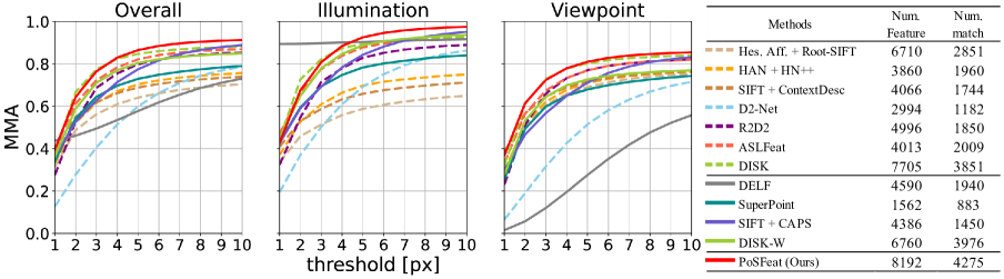
Figure 5: Results achieved on the HPatches dataset [3]. Mean match accuracy (MMA) achieved at different thresholds are illustrated. Learning based methods with weak supervision are shown in solid lines while other methods are shown in dashed lines. The numbers of keypoints and matches for each method are also reported.

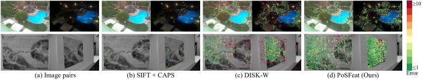
Figure 6: Visualization results achieved on HPatches. For simplicity, only successfully matched keypoints are shown and colored according to their match errors. The colorbar is shown on the right. Best viewed in color.

4.2.1 Feature Matching

Settings. We first evaluate our method on the widely used HPatches dataset [3].Following D2-Net [13], 8 high-resolution scenes are removed and the remaining 52 scenes with illumination changes and 56 scenes with viewpoint changes are included for evaluation. Mean matching accuracy (MMA) [13] with thresholds ranging from 1 to 10 is used for evaluation. We also use a weighted sum of MMA at different thresholds for overall evaluation:

$${\rm MMAscore}=\frac{\sum_{{\rm thr}\in[1,10]}(2-0.1\cdot{\rm thr})\cdot{\rm MMA@thr}}{\sum_{{\rm thr}\in[1,10]}(2-0.1\cdot{\rm thr})}.$$ (12)

Three families of methods are included for comparison:

• Patch-based methods: Hessian-Affine keypoints [26] with Root-SIFT [2] (Hes. Aff. + Root-SIFT), affine region detector HesAffNet [28] with HardNet++ [27] (HAN + HN++), and SIFT [22] with ContextDesc [23] (SIFT + ContextDesc).

• Fully supervised dense feature methods: D2-Net [13], R2D2 [34], ASLFeat [24], and DISK [46].

• Weakly supervised dense feature methods: DELF [30], SuperPoint [12], DISK-W [46], and SIFT with CAPS [47] (SIFT + CAPS).

Methods	MMAscore Overall	MMAscore Illumination	MMAscore Viewpoint
Hes. Aff. + Root-SIFT [2]	0.584	0.544	0.624
HAN  [28] + HN++ [27]	0.633	0.634	0.633
SIFT [22] + ContextDesc [23]	0.636	0.613	0.657
D2Net [13]	0.519	0.605	0.440
R2D2 [34]	0.695	0.727	0.665
ASLFeat [24]	0.739	0.795	0.687
DISK [46]	0.763	0.813	0.716
DELF [30]	0.571	0.903	0.262
SuperPoint [12]	0.658	0.715	0.606
SIFT [22] + CAPS [47]	0.699	0.764	0.639
DISK-W [46]	0.719	0.803	0.649
PoSFeat (Ours)	0.775	0.826	0.728

Table 1: MMAscore results achieved by different methods on the HPatches dataset [3]. The MMAscores are calculated from Fig. 5.

Results. As shown in Fig. 5 and Table 1, the proposed PoSFeat outperforms all previous works, with the highest MMAscore being achieved. Compared to existing weakly supervised methods, our method produces significant performance improvements. Specifically, our method outperforms DISK-W by notable margins under both illumination (0.826 vs. 0.803) and viewpoint (0.728 vs. 0.649) changes, and therefore achieves higher overall MMAscore (0.775 vs. 0.719). We also visualize the matching results in Fig. 6. It can be seen that our PoSFeat produces more reasonable keypoints and less wrong matches. Compared to fully supervised methods, our method still performs favorably with higher MMA scores. This clearly demonstrates the superiority of our method. Note that, because DELF detects keypoints in a low resolution feature map with a fixed grid, it produces the best results under illumination change. However, our method significantly surpasses DELF under viewpoint change (0.728 vs. 0.262) and achieves much better overall performance (0.775 vs. 0.571).

4.2.2 Visual Localization

Settings. We then evaluate our method on the visual localization task with the Aachen Day-Night dataset [51].We adopt the official visual localization pipeline used in the local feature challenge of workshop on long-term visual localization under changing conditions. This challenge only evaluates the pose of night-time query images. Accuracy with different thresholds are used as metrics, including (0.5m, 2^∘), (1m, 5^∘), and (5m, 10^∘).

We compare our method with two families of methods:

• Local feature methods: D2-Net [13], SuperPoint [12], R2D2 [34], ASLFeat [24], ISRF [25], and LISRD [33].

• Matcher methods: DualRC-Net [20], SuperGlue [37] + SuperPoint, SparseNCNet [35], LoFTR [42], Patch2Pix [53], and SGMNet [10] + SuperPoint. As mentioned in Sec 2.4, matchers are the cooperators instead of the direct competitors of local features. Therefore, we group them separately.

Method	Aachen Day-Night v1			Aachen Day-Night v1.1
	(0.5m,2∘)	(1m,5∘)	(5m, 10∘)	(0.5m,2∘)	(1m,5∘)	(5m, 10∘)
SP [12]	74.5	78.6	89.8	-	-	-
D2-Net [13]	74.5	86.7	100	-	-	-
R2D2 [34]	76.5	90.8	100	71.2	86.9	97.9
ASLFeat [24]	81.6	87.8	100	-	-	-
ISRF [25]	-	-	-	69.1	87.4	98.4
LISRD [33]	-	-	-	73.3	86.9	97.9
PoSFeat (Ours)	81.6	90.8	100	73.8	87.4	98.4
DualRC-Net [20]	-	-	-	71.2	86.9	97.9
SP+SuperGlue [37]	79.6	90.8	100	73.3	88.0	98.4
Sparse-NCNet [35]	76.5	84.7	98.0	-	-	-
LoFTR [42]	-	-	-	72.8	88.5	99.0
Patch2Pix [53]	79.6	87.8	100	-	-	-
SP+SGMNet [10]	77.6	88.8	99.0	72.3	85.3	97.9

Table 2: Results achieved by different methods on the Aachen Day-Night dataset [51]. ‘LISRD’ represents LISRD with SuperPoint keypoints and AdaLAM [9]. Two categories of methods are presented, including feature methods (top) and matchers (bottom).

Results. As shown in Table 2, our PoSFeat achieves the state-of-the-art performance among the feature methods. Specifically, on Aachen Day-Night v1, our method achieves the best accuracy in terms of all metrics. Note that, although ASLFeat is a fully supervised method, our PoSFeat still outperforms it on (1m, 5^∘). On Aachen Day-Night v1.1, our method also produces the best performance in all metrics. Note that, although R2D2 [34], ISRF [25], and LISRD [33] are fully-supervised and trained on the Aachen Day-Night dataset, our PoSFeat still achieves better results. We additionally include matcher methods for further comparison. Although these methods take pairs of images as inputs, our PoSFeat achieves comparable or even better performance.

Subset	Method	# Imgs	# Pts	Track Length	Reproj. Err. (px)
South Building (128 imgs)	Root-SIFT [2, 22]	128	108k	6.32	0.55
	SuperPoint [12]	128	160k	7.83	0.92
	RFP [6]	128	102k	7.86	0.88
	DISK [46]	128	115k	9.91	0.59
	DISK-W [46]	128	154k	9.63	0.63
	PoSFeat (Ours)	128	148k	9.47	0.58
Madrid Metropolis (1344 imgs)	Root-SIFT [2, 22]	500	116k	6.32	0.60
	SuperPoint [12]	438	29k	9.03	1.02
	D2-Net [13]	501	84k	6.33	1.28
	ASLFeat [24]	613	96k	8.76	0.90
	CAPS [47]	851	242k	6.16	1.03
	CoAM [49]	702	256k	6.09	1.30
	PoSFeat (Ours)	419	72k	9.18	0.86
Gendar- menmarkt (1463 imgs)	Root-SIFT [2, 22]	1035	339k	5.52	0.70
	SuperPoint [12]	967	93k	7.22	1.03
	D2-Net [13]	1053	250k	5.08	1.19
	ASLFeat [24]	1040	221k	8.72	1.00
	CAPS [47]	1179	627k	5.31	1.00
	CoAM [49]	1072	570k	6.60	1.34
	PoSFeat (Ours)	956	240k	8.40	0.92
Tower of London (1576 imgs)	Root-SIFT [2, 22]	806	239k	7.76	0.61
	SuperPoint [12]	681	52k	8.67	0.96
	D2-Net [13]	785	180k	5.32	1.24
	ASLFeat [24]	821	222k	12.52	0.92
	CAPS [47]	1104	452k	5.81	0.98
	CoAM [49]	804	239k	5.82	1.32
	PoSFeat (Ours)	778	262k	11.64	0.90

Table 3: Results achieved by different methods on the ETH local feature benchmark.

4.2.3 3D Reconstruction

Settings. We finally evaluate our method on the 3D reconstruction task. We conduct experiments on the ETH local feature benchmark [41]. Four metrics are used for evaluation, including the number of registered images (# Imgs), the number of sparse points (# Pts), track length, and the mean reprojection error (Reproj. Err.).

Four families of methods were included for comparison:

• Patch-based method: Root-SIFT [2, 22].

• Fully supervised dense feature methods: Reinforced Feature Points [6] (RFP), DISK [46], DISK-W [46], D2-Net [13], and ASLFeat [24].

• Weakly supervised dense feature methods: SuperPoint [12] and CAPS [47].

• Fully supervised matcher method: CoAM [49].

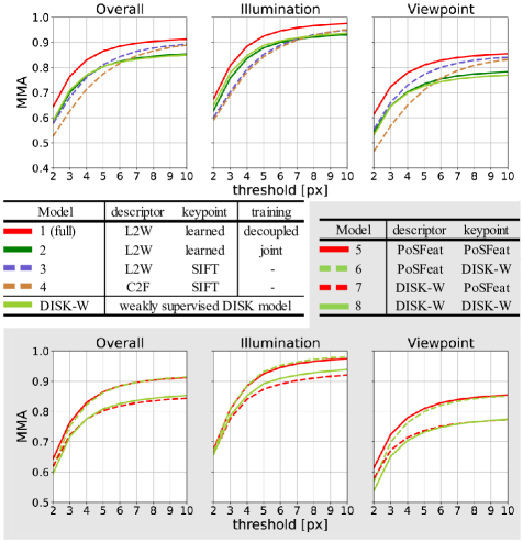
Figure 7: Ablation results on HPatches. “L2W” denotes our line-to-window search strategy (illustrated in Fig 4(b)) and “C2F” denotes the coarse-to-fine search strategy [47] (illustrated in Fig 4(a)). “learned” means that the keypoints are generated by a detection network and “SIFT” mean that SIFT keypoints (OpenCV default settings) are used. “decoupled” means the proposed decoupled training pipeline is adopted and ‘joint’ means the description network and the detection network are jointly optimized.

Results. As shown in Table 3, our method performs favorably against previous methods on the 3D reconstruction task. Specifically, our method produces the lowest reprojection error among all learning-based methods. Moreover, our method achieves the best or second best performance in terms of track length, which demonstrates that our keypoints are robust and thus can be tracked across a large amount of images.

4.3 Ablation Study

In this section, we first conduct ablation experiments on the HPatches dataset [3] to demonstrate the effectiveness of our decoupled training describe-then-detect pipeline and line-to-window search strategy. Then, we conduct experiments to study the effectiveness of hyper-parameters in our method, i.e., the number of points sampled from the epipolar line $N_{line}$ and the window size $w_{patch}$. Results and model settings are shown in Fig. 7 and Table 4.

Decoupled Training Describe-then-Detect Pipeline. We first constructed a network variant (Model 2) following the joint training describe-then-detect pipeline. That is, the description network and the detection network are jointly optimized. Then, we developed Model 3 based on the detect-then-describe pipeline. Specifically, the description network is combined with SIFT keypoints in Model 3.

As shown in Fig. 7, with only weak supervision, the ambiguity during optimization limits the performance of joint training describe-then-detect approaches (Model 2 and DISK-W). Moreover, Model 2 is even inferior to Model 3 under viewpoint change. Compared to Models 2 and 3, Model 1 with our decoupled training describe-then-detect pipeline produces much higher accuracy. This clearly demonstrates that our decoupled training describe-then-detect pipeline is well suitable to weakly supervised learning to achieve superior performance.

We further test different combinations of keypoints and descriptors (Models 5-8). It can be observed that the improvement mainly comes from the descriptor, and the keypoints are slightly improved on the viewpoint change. Besides, we also illustrate the keypoints produced by our method and DISK-W in Fig. 1. DISK-W generates considerable inaccurate keypoints out of objects (e.g., in the sky). In contrast, our model detects more reasonable keypoints. That is because those mismatched descriptors and erroneous keypoints produced from two different components do not influence each other within our decoupled training describe-then-detect pipeline.

	0.075	0.100	0.125
75	0.7703	0.7705	0.7666
100	0.7726	0.7748	0.7732
125	0.7732	0.7745	0.7744

Table 4: MMAscore achieved by our description network with different values of $N_{line}$ and $w_{patch}$ on the HPatches dataset.

Line-to-Window Search Strategy. To validate the effectiveness of our line-to-window search strategy, we developed a network variant (Model 4) by replacing our search strategy with a coarse-to-fine one (as proposed in [47], illustrated in Fig. 4(a)). For fair comparison with Model 3, SIFT keypoints are employed in this network variant. It can be observed that Model 3 outperforms Model 4 by significant margins. That is because, our line-to-window search strategy can make full use of the geometry information of camera poses to reduce the search space for accurate localization of correspondences. Consequently, higher accuracy can be achieved.

Number of Sampled Points $N_{line}$ and Window Size $w_{patch}$. We conduct experiments to study the effects of $N_{line}$ and $w_{patch}$ during our line-to-window search. More sampled points and a large window size are beneficial to the performance at the expense of higher computational cost. To achieve a trade-off between performance and computational complexity, $w_{patch}=0.100$ and $N_{line}=100$ are used as the default setting.

5 Conclusion

In this paper, we introduce a decoupled training describe-then-detect pipeline tailored for weakly supervised local feature learning. Within our pipeline, the detection network is decoupled from the description network and postponed until discriminative and robust descriptors are obtained. In addition, we propose a line-to-window search strategy to explicitly use the camera pose information to reduce search space for better descriptor learning. Extensive experiments show that our method achieves the state-of-the-art performance on three different evaluation frameworks and significantly closes the gap between fully-supervised and weakly supervised methods.

Acknowledgement. This work was partially supported by the National Key Research and Development Program of China (No. 2021YFB3100800), the Shenzhen Science and Technology Program (No. RCYX20200714114641140), and National Natural Science Foundation of China (No. U20A20185, 61972435, 62132021).

References

- [1] Sameer Agarwal, Yasutaka Furukawa, Noah Snavely, Ian Simon, Brian Curless, Steven M Seitz, and Richard Szeliski. Building Rome in a Day. Communications of the ACM, 54(10):105–112, 2011.
- [2] Relja Arandjelović and Andrew Zisserman. Three Things Everyone Should Know to Improve Object Retrieval. In Proceedings of the IEEE/CVF Conference on Computer Vision and Pattern Recognition (CVPR), pages 2911–2918, 2012.
- [3] Vassileios Balntas, Karel Lenc, Andrea Vedaldi, and Krystian Mikolajczyk. HPatches: A Benchmark and Evaluation of Handcrafted and Learned Local Descriptors. In Proceedings of the IEEE/CVF Conference on Computer Vision and Pattern Recognition (CVPR), 2017.
- [4] Axel Barroso-Laguna, Edgar Riba, Daniel Ponsa, and Krystian Mikolajczyk. Key.Net: Keypoint Detection by Handcrafted and Learned CNN Filters. In Proceedings of the IEEE/CVF International Conference on Computer Vision (ICCV), pages 5836–5844, 2019.
- [5] Herbert Bay, Tinne Tuytelaars, and Luc Van Gool. SURF: Speeded Up Robust Features. In Proceedings of the European Conference on Computer Vision (ECCV), pages 404–417, 2006.
- [6] Aritra Bhowmik, Stefan Gumhold, Carsten Rother, and Eric Brachmann. Reinforced Feature Points: Optimizing Feature Detection and Description for a High-Level Task. In Proceedings of the IEEE/CVF Conference on Computer Vision and Pattern Recognition (CVPR), pages 4948–4957, 2020.
- [7] Sudong Cai, Yulan Guo, Salman Khan, Jiwei Hu, and Gongjian Wen. Ground-to-aerial image geo-localization with a hard exemplar reweighting triplet loss. In Proceedings of the IEEE/CVF International Conference on Computer Vision (ICCV), pages 8391–8400, 2019.
- [8] Michael Calonder, Vincent Lepetit, Mustafa Ozuysal, Tomasz Trzcinski, Christoph Strecha, and Pascal Fua. BRIEF: Computing a Local Binary Descriptor Very Fast. IEEE Transactions on Pattern Analysis and Machine Intelligence (TPAMI), 34(7):1281–1298, 2011.
- [9] Luca Cavalli, Viktor Larsson, Martin Ralf Oswald, Torsten Sattler, and Marc Pollefeys. Handcrafted Outlier Detection Revisited. In Proceedings of the European Conference on Computer Vision (ECCV), pages 770–787, 2020.
- [10] Hongkai Chen, Zixin Luo, Jiahui Zhang, Lei Zhou, Xuyang Bai, Zeyu Hu, Chiew-Lan Tai, and Long Quan. Learning to Match Features with Seeded Graph Matching Network. In Proceedings of the IEEE/CVF International Conference on Computer Vision (ICCV), pages 6301–6310, 2021.
- [11] Peter Hviid Christiansen, Mikkel Fly Kragh, Yury Brodskiy, and Henrik Karstoft. UnsuperPoint: End-to-end Unsupervised Interest Point Detector and Descriptor. arXiv preprint arXiv:1907.04011, 2019.
- [12] Daniel DeTone, Tomasz Malisiewicz, and Andrew Rabinovich. SuperPoint: Self-Supervised Interest Point Detection and Description. In Proceedings of the IEEE/CVF Conference on Computer Vision and Pattern Recognition Workshops (CVPRW), pages 224–236, 2018.
- [13] Mihai Dusmanu, Ignacio Rocco, Tomas Pajdla, Marc Pollefeys, Josef Sivic, Akihiko Torii, and Torsten Sattler. D2-Net: A Trainable CNN for Joint Detection and Description of Local Features. In Proceedings of the IEEE/CVF Conference on Computer Vision and Pattern Recognition (CVPR), 2019.
- [14] Patrick Ebel, Anastasiia Mishchuk, Kwang Moo Yi, Pascal Fua, and Eduard Trulls. Beyond Cartesian Representations for Local Descriptors. In Proceedings of the IEEE/CVF International Conference on Computer Vision (ICCV), pages 253–262, 2019.
- [15] Steve R Gunn. Edge Detection Error in the Discrete Laplacian of Gaussian. In Proceedings of the International Conference on Image Processing (ICIP), volume 2, pages 515–519. IEEE, 1998.
- [16] Yulan Guo, Michael Choi, Kunhong Li, Farid Boussaid, and Mohammed Bennamoun. Soft exemplar highlighting for cross-view image-based geo-localization. IEEE Transactions on Image Processing (TIP), 31:2094–2105, 2022.
- [17] Chris Harris, Mike Stephens, et al. A Combined Corner and Edge Detector. In Alvey vision conference, volume 15, pages 147–151. Citeseer, 1988.
- [18] Yuhe Jin, Dmytro Mishkin, Anastasiia Mishchuk, Jiri Matas, Pascal Fua, Kwang Moo Yi, and Eduard Trulls. Image Matching Across Wide Baselines: From Paper to Practice. International Journal of Computer Vision (IJCV), 129(2):517–547, 2021.
- [19] Stefan Leutenegger, Margarita Chli, and Roland Y Siegwart. BRISK: Binary Robust Invariant Scalable Keypoints. In Proceedings of the IEEE/CVF International Conference on Computer Vision (ICCV), pages 2548–2555. IEEE, 2011.
- [20] Xinghui Li, Kai Han, Shuda Li, and Victor Prisacariu. Dual-Resolution Correspondence Networks. In Advances in Neural Information Processing Systems (NeurIPS), volume 33, 2020.
- [21] Zhengqi Li and Noah Snavely. MegaDepth: Learning Single-View Depth Prediction From Internet Photos. In Proceedings of the IEEE/CVF Conference on Computer Vision and Pattern Recognition (CVPR), pages 2041–2050, 2018.
- [22] David G Lowe. Distinctive Image Features from Scale-Invariant Keypoints. International Journal of Computer Vision (IJCV), 60(2):91–110, 2004.
- [23] Zixin Luo, Tianwei Shen, Lei Zhou, Jiahui Zhang, Yao Yao, Shiwei Li, Tian Fang, and Long Quan. ContextDesc: Local Descriptor Augmentation with Cross-Modality Context. In Proceedings of the IEEE/CVF Conference on Computer Vision and Pattern Recognition (CVPR), 2019.
- [24] Zixin Luo, Lei Zhou, Xuyang Bai, Hongkai Chen, Jiahui Zhang, Yao Yao, Shiwei Li, Tian Fang, and Long Quan. ASLFeat: Learning Local Features of Accurate Shape and Localization. In Proceedings of the IEEE/CVF Conference on Computer Vision and Pattern Recognition (CVPR), 2020.
- [25] Iaroslav Melekhov, Gabriel J Brostow, Juho Kannala, and Daniyar Turmukhambetov. Image Stylization for Robust Features. arXiv preprint arXiv:2008.06959, 2020.
- [26] Krystian Mikolajczyk and Cordelia Schmid. Scale & Affine Invariant Interest Point Detectors. International Journal of Computer Vision (IJCV), 60(1):63–86, 2004.
- [27] Anastasiia Mishchuk, Dmytro Mishkin, Filip Radenovic, and Jiri Matas. Working Hard to Know Your Neighbor's Margins: Local Descriptor Learning Loss. In Advances in Neural Information Processing Systems (NeurIPS), volume 30, 2017.
- [28] Dmytro Mishkin, Filip Radenovic, and Jiri Matas. Repeatability Is Not Enough: Learning Affine Regions via Discriminability. In Proceedings of the European Conference on Computer Vision (ECCV), pages 284–300, 2018.
- [29] Raul Mur-Artal and Juan D Tardós. ORB-SLAM2: An Open-Source SLAM System for Monocular, Stereo, and RGB-D Cameras. IEEE Transactions on Robotics (TR), 33(5):1255–1262, 2017.
- [30] Hyeonwoo Noh, Andre Araujo, Jack Sim, Tobias Weyand, and Bohyung Han. Large-Scale Image Retrieval With Attentive Deep Local Features. In Proceedings of the IEEE/CVF International Conference on Computer Vision (ICCV), pages 3456–3465, 2017.
- [31] Yuki Ono, Eduard Trulls, Pascal Fua, and Kwang Moo Yi. LF-Net: Learning Local Features from Images. In Advances in Neural Information Processing Systems (NeurIPS), 2018.
- [32] Udit Singh Parihar, Aniket Gujarathi, Kinal Mehta, Satyajit Tourani, Sourav Garg, Michael Milford, and K Madhava Krishna. RoRD: Rotation-Robust Descriptors and Orthographic Views for Local Feature Matching. In Proceedings of the IEEE/RSJ International Conference on Intelligent Robots and Systems (IROS), 2021.
- [33] Rémi Pautrat, Viktor Larsson, Martin R Oswald, and Marc Pollefeys. Online Invariance Selection for Local Feature Descriptors. In Proceedings of the European Conference on Computer Vision (ECCV), pages 707–724, 2020.
- [34] Jerome Revaud, Cesar De Souza, Martin Humenberger, and Philippe Weinzaepfel. R2D2: Reliable and Repeatable Detector and Descriptor. In Advances in Neural Information Processing Systems (NeurIPS), volume 32, pages 12405–12415, 2019.
- [35] Ignacio Rocco, Relja Arandjelović, and Josef Sivic. Efficient neighbourhood consensus networks via submanifold sparse convolutions. In Proceedings of the European Conference on Computer Vision (ECCV), pages 605–621. Springer, 2020.
- [36] Ethan Rublee, Vincent Rabaud, Kurt Konolige, and Gary Bradski. ORB: An Efficient Alternative to SIFT or SURF. In Proceedings of the IEEE/CVF International Conference on Computer Vision (ICCV), pages 2564–2571. IEEE, 2011.
- [37] Paul-Edouard Sarlin, Daniel DeTone, Tomasz Malisiewicz, and Andrew Rabinovich. SuperGlue: Learning Feature Matching With Graph Neural Networks. In Proceedings of the IEEE/CVF Conference on Computer Vision and Pattern Recognition (CVPR), pages 4938–4947, 2020.
- [38] Torsten Sattler, Bastian Leibe, and Leif Kobbelt. Improving Image-Based Localization by Active Correspondence Search. In Proceedings of the European Conference on Computer Vision (ECCV), pages 752–765, 2012.
- [39] Nikolay Savinov, Akihito Seki, Lubor Ladicky, Torsten Sattler, and Marc Pollefeys. Quad-Networks: Unsupervised Learning to Rank for Interest Point Detection. In Proceedings of the IEEE/CVF Conference on Computer Vision and Pattern Recognition (CVPR), pages 1822–1830, 2017.
- [40] Johannes L Schonberger and Jan-Michael Frahm. Structure-from-Motion Revisited. In Proceedings of the IEEE/CVF Conference on Computer Vision and Pattern Recognition (CVPR), pages 4104–4113, 2016.
- [41] Johannes L Schonberger, Hans Hardmeier, Torsten Sattler, and Marc Pollefeys. Comparative Evaluation of Hand-Crafted and Learned Local Features. In Proceedings of the IEEE/CVF Conference on Computer Vision and Pattern Recognition (CVPR), pages 1482–1491, 2017.
- [42] Jiaming Sun, Zehong Shen, and Yuang Wang. LoFTR: Detector-Free Local Feature Matching With Transformers. In Proceedings of the IEEE/CVF Conference on Computer Vision and Pattern Recognition (CVPR), pages 8922–8931, 2021.
- [43] Ilya Sutskever, James Martens, George Dahl, and Geoffrey Hinton. On the Importance of Initialization And Momentum in Deep Learning. In Proceedings of the International Conference on Machine Learning (ICML), pages 1139–1147, 2013.
- [44] Yurun Tian, Xin Yu, Bin Fan, Fuchao Wu, Huub Heijnen, and Vassileios Balntas. SOSNet: Second Order Similarity Regularization for Local Descriptor Learning. In Proceedings of the IEEE/CVF Conference on Computer Vision and Pattern Recognition (CVPR), pages 11016–11025, 2019.
- [45] Carl Toft, Will Maddern, Akihiko Torii, Lars Hammarstrand, Erik Stenborg, Daniel Safari, Masatoshi Okutomi, Marc Pollefeys, Josef Sivic, Tomas Pajdla, et al. Long-Term Visual Localization Revisited. IEEE Transactions on Pattern Analysis and Machine Intelligence (TPAMI), 2020.
- [46] Michał J. Tyszkiewicz, Pascal Fua, and Eduard Trulls. DISK: Learning Local Features with Policy Gradient. In Advances in Neural Information Processing Systems (NeurIPS), volume 33, 2020.
- [47] Qianqian Wang, Xiaowei Zhou, Bharath Hariharan, and Noah Snavely. Learning Feature Descriptors Using Camera Pose Supervision. In Proceedings of the European Conference on Computer Vision (ECCV), volume 12346, pages 757–774, 2020.
- [48] Xupeng Wang, Ferdous Ahmed Sohel, Mohammed Bennamoun, Yulan Guo, and Hang Lei. Persistence-based interest point detection for 3D deformable surface. In International Conference on Computer Graphics Theory and Applications (GRAPP), pages 58–69, 2017.
- [49] Olivia Wiles, Sebastien Ehrhardt, and Andrew Zisserman. Co-Attention for Conditioned Image Matching. In Proceedings of the IEEE/CVF Conference on Computer Vision and Pattern Recognition (CVPR), pages 15920–15929, 2021.
- [50] Kwang Moo Yi, Eduard Trulls, Vincent Lepetit, and Pascal Fua. LIFT: Learned Invariant Feature Transform. In Proceedings of the European Conference on Computer Vision (ECCV), pages 467–483, 2016.
- [51] Zichao Zhang, Torsten Sattler, and Davide Scaramuzza. Reference Pose Generation for Long-term Visual Localization via Learned Features and View Synthesis. International Journal of Computer Vision (IJCV), 129(4):821–844, 2021.
- [52] Yong Zhao, Shibiao Xu, Shuhui Bu, Hongkai Jiang, and Pengcheng Han. GSLAM: A General SLAM Framework and Benchmark. In Proceedings of the IEEE/CVF International Conference on Computer Vision (ICCV), pages 1110–1120, 2019.
- [53] Qunjie Zhou, Torsten Sattler, and Laura Leal-Taixe. Patch2pix: Epipolar-guided pixel-level correspondences. In Proceedings of the IEEE/CVF Conference on Computer Vision and Pattern Recognition (CVPR), pages 4669–4678, 2021.