ROTEC: Robust to Early Termination Command Governor for Systems with Limited Computing Capacity111This research has been supported by National Science Foundation under award numbers ECCS-1931738, ECCS-1932530, and CMMI-1904394.
Abstract
A Command Governor (CG) is an optimization-based add-on scheme to a nominal closed-loop system. It is used to enforce state and control constraints by modifying reference commands. This paper considers the implementation of a CG on embedded processors that have limited computing resources and must execute multiple control and diagnostics functions; consequently, the time available for CG computations is limited and may vary over time. To address this issue, a robust to early termination command governor is developed which embeds the solution of a CG problem into the internal states of a virtual continuous-time dynamical system which runs in parallel to the process. This virtual system is built so that its trajectory converges to the optimal solution (with a tunable convergence rate), and provides a sub-optimal but feasible solution whenever its evolution is terminated. This allows the designer to implement a CG strategy with a small sampling period (and consequently with a minimum degradation in its performance), while maintaining its constraint-handling capabilities. Simulations are carried out to assess the effectiveness of the developed scheme in satisfying performance requirements and real-time schedulability conditions for a practical vehicle rollover example.
keywords:
Cyber–physical systems , Safety-critical control schemes , Command governor , Real-time schedulability , Vehicle rollover prevention1 Introduction
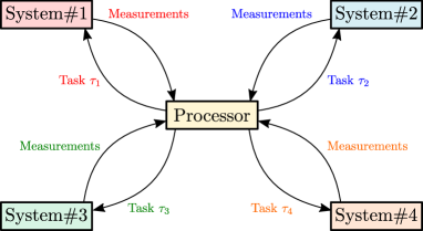
A common aspect of today’s Cyber–Physical Systems (CPSs) is that multiple safety-critical controllers/control systems responsible for different system functions may execute in a shared processing unit—see Figure 1. Examples of such systems can be found in safety-critical applications like aircraft, autonomous vehicles, medical devices, and autonomous robots.
(a)
(b)
Three related issues that should be addressed carefully when designing such CPSs with multiple control systems are: 1) system performance; 2) system safety; and 3) real-time schedulability. System performance refers to the degree to which the control objectives of the individual control systems are achieved, which can be indicated by various measures of cost, efficiency, accuracy, etc. System safety refers to the satisfaction of the operational constraints and requirements. Real-time schedulability assures that timing requirements of different control systems informing the CPS are satisfied.
1.1 Prior Work on Real-Time Scheduling
The implementation of controllers can be seen as the problem of executing recurrent (periodic) tasks [1] on a resource-constrained processor. The real-time scheduling literature (e.g., [2]) provides a wide range of schedulability analysis techniques based upon the Earliest Deadline First (EDF) policy [1, 3] to address this problem. These techniques primarily emphasize the scheduling aspects and stabilization of control systems under cyber constraints (e.g., limited computational time and end-to-end delay); to the best of our knowledge, prior real-time scheduling techniques do not explicitly address/ensure physical constraints222Throughout this paper, by “constraints” we mean constraints on system input and/or state variables. satisfaction (e.g., hard limits on system input, state, and output variables).
Existing real-time schedulability analysis techniques may be roughly classified into two groups. The first group (e.g., [4, 5, 6]) determines the worst-case execution time of each task, and then determines the sampling periods for each task such that the real-time schedulability conditions are satisfied.
A main shortcoming of this approach arises from the variability and unpredictability of task execution times, particularly on modern processors [7]. As a result, the worst-case execution times of the tasks are computed conservatively. This tends to severely under-utilize the computational resources, and requires assignment of large sampling periods to the tasks, which can lead to control performance degradation. See [8] for more details about the trade-off between resources and control performance in embedded control systems. Though methods to determine sampling periods which ensures stability and reduce the impact on system performance have been proposed in the prior literature (e.g., [9, 10, 11, 12, 13]), this paper addresses the impact of limited computing capacity on the ability to satisfy physical constraints (i.e., constraints on input and/or state variables) with the Command Governor scheme; this problem is different and has not been addressed in the prior literature.
The second group of more recent schedulability analysis techniques involves task scheduling based upon a relaxed upper bound on their execution times. In this case, first, an optimistic upper bound on the execution time of each task is estimated, within which most invocations of the task are deemed likely to complete. Sampling periods for each task are then computed based upon these optimistic upper bounds so to satisfy real-time schedulability conditions. At run-time, if the execution time of a task exceeds the determined upper-bound at any sampling instant, the processor allows the task to complete, which delays the execution of other tasks. This can be seen as an unwanted increase in the sampling periods of all tasks. To compensate for the impact of this increase, the control parameters for all control systems are modified at the next sampling instant. This approach has been investigated in [14, 15], and shown to lead to better performance and reduce under-utilization of computational resources. To avoid adding extra computational burden, the modifications can be computed offline for the set of all possible cases and stored for online use. A method for reducing the number of controllers to be designed offline, while still guaranteeing specified control performance, is presented in [16]. However, in general, there are no systematic methods to compute the modifications, and even no guarantees for the existence of such modifications. Furthermore, proposed strategies do not enforce physical constraints.
The problem of control-scheduling co-design under different types of cyber constraints is addressed in [17, 18, 19]. In particular, stabilization of a control system in presence of limited execution time has been studied in [17], where the authors present an event-triggered scheduler that decides which task should be executed at any given instant. The authors of [18] present a heuristic optimization method to optimize the end-to-end timing constraint (i.e., loop processing time and input-to-output latency) for a given control performance specification. A server-based resource reservation mechanism is proposed in [19] to ensure stability in the presence of server bandwidth constraints. However, physical constraints (i.e., constraints on input and/or state variables) have not been considered in the above-mentioned references.
Another policy used to address the real-time schedulability in CPSs is the Fixed Priority Preemptive Scheduling (FPPS) policy [20, 21]. In this policy, the processor executes the highest priority task of all those tasks that are currently ready to execute. Though different methods have been proposed to assign priorities to ensure that all tasks will execute (e.g., [22, 23]), if a critical task is the one with lower priority and other tasks are always schedulable without that task, the lower-priority task could wait for an unpredictable amount of time. This obviously degrades the control performance, and may even lead to constraints violation.
1.2 Prior Work on Optimization-Based Constrained Control of Systems With Limited Computing Capacity
As mentioned above, safety in this paper is related to the constraint enforcement. The literature on constrained control has been dominated by optimization-based techniques, such as Model Predictive Control (MPC) [24, 25], Reference/Command Governors (RG/CG) [26], and Control Barrier Functions [27]. However, the use of online optimization is computationally intensive and creates practical challenges when they are employed in a CPS with limited computational power.
Another approach to implement optimization-based control laws for system with constraints is to pre-compute them offline and store them in memory for future use. This idea is adopted in explicit MPC [28]. However, even in the case of linear quadratic MPC, explicit MPC can be more memory and computation time consuming for larger state dimensional problems or problems with a large number of constraints as compared to the onboard optimization based methods. Furthermore, it is not robust with respect to early/premature termination of the search for the polyhedral region containing the current state.
Another possible way to address limited computing power is to resort to triggering, as in self-triggered [29] and event-triggered [30, 31] optimization-based constrained control. However, there is no guarantee that sufficient computational power will be available when the triggering mechanism invokes simultaneously multiple controllers.
Another way to address limited computational power in optimization-based constrained control schemes is to perform a fixed number of iterations to approximately track the solution of the associated optimization problem. This approach has been extensively investigated for MPC [32, 33]. For instance, [34] pursues the analysis of the active-set methods to determine a bound on the number of iterations. However, there is no guarantee that required iterations can be carried out in the available time in a shared processing unit. The dynamically embedded MPC is introduced in [35], where the processor, instead of solving the MPC iteration, runs a virtual dynamical system whose trajectory converges to the optimal solution of the MPC problem. Although employing warm-starting [36] can improve convergence of the virtual dynamical system in dynamically embedded MPC, guaranteeing recursive feasibility (i.e., remaining feasible indefinitely) with this scheme is challenging, as a sudden change in the reference signal can drastically change the problem specifics, e.g., the terminal set may not be reachable anymore within the given prediction horizon. To address this issue, in [37], the dynamically embedded MPC is augmented with an Explicit Reference Governor (ERG) [38, 39, 40]; however, this may lead to conservative (slow) response due to conservatism of ERG.
A CG supervisory scheme is presented in [41], where different CG problems are designed for different operating points of the system, and a switching mechanism is proposed to switch between CG schemes. However, the effects of early termination of the computations on the CG schemes has not been considered in [41]. In [42], a one-layer recurrent neural network is proposed to solve a CG problem in finite time. However, [42] does not address the variability and unpredictability of the available computing time for CG schemes when implemented in a shared processing unit and, in particular, situations when the available time is less that the required time for convergence.
1.3 Proposed Solution
A CG is an optimization-based add-on scheme to a nominal closed-loop system used to modify the reference command in order to satisfy state and input constraints. In this paper, we develop ROTEC (RObust to early TErmination Command governor), which is based on the use of primal-dual flow algorithm to define a virtual continuous-time dynamical system whose trajectory tracks the optimal solution of the CG. ROTEC runs until available time for execution runs out (that may not be known in advance) and the solution is guaranteed to enforce the constraints despite any early termination. ROTEC can guarantee safety while addressing system performance. Also, it guarantees recursive feasibility. This feature allows to satisfy the real-time schedulability condition, even when numerous safety-critical control systems are implemented on a processor with very limited computational power.
In this paper, ROTEC is introduced as a continuous-time scheme. This facilitates the analysis and the derivation of its theoretical properties. Our numerical experiments show that these properties are maintained when ROTEC is implemented in discrete time with a sufficiently small sampling period. This is not dissimilar to how control schemes are derived and analyzed. We leave the study of theoretical guarantees for the discrete-time implementation to future work.
1.4 Contribution
To the best of our knowledge, this paper is the first that ensures robustness to early termination for CG schemes. This feature allows us to address real-time schedulability in CPSs, while ensuring constraints satisfaction at all times. In particular, it is shown analytically that ROTEC ensures the safe and efficient operation of a CPS. The main contributions are: 1) development of ROTEC; 2) demonstration that it enforces the constraints robustly with respect to the time available for computations; and 3) evaluation of its effectiveness for vehicle rollover prevention.
Our approach to CG implementation is inspired by [43, 44] in exploiting barrier functions and the primal-dual continuous-time flow algorithm, but addresses a different problem. Our proofs of convergence are inspired by Lyapunov-based approaches in [35, 37, 45], but once again explored for a different problem.
1.5 Organization
The rest of the paper is organized as follows. Section 2 formulates the problem, and discusses the control requirements and real-time schedulability conditions. Section 3 describes the conventional CG scheme. Section 4 develops ROTEC, proves its properties, and discusses its initialization. In Section 5, a simulation study of vehicle rollover is reported to validate ROTEC. Finally, Section 6 concludes the paper.
1.6 Notation
We use to denote continuous time, to denote sampling instants, to denote predictions made at each sampling instant, and to denote the auxiliary time scale that ROTEC spends on solving the CG problem. and 0 indicate, respectively, the identity and zero matrices with appropriate dimensions. In this paper, .
2 Problem Formulation
This section gives details about the considered CPS setting, highlights the practical challenges, and explains how we address the challenges.
2.1 Setting
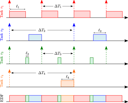
We consider a CPS comprising controllers implemented on a single processing unit. From a real-time computing perspective, this can be seen as a set of tasks running on a single processor. We denote the tasks by , where task performs a specific action for the -th control system. The task is represented by the 2-tuple , where is the worst-case execution time and is the sampling period. Suppose that tasks correspond to pivotal actions with fixed and pre-determined sampling periods, and task implements a CG strategy. This setting is considered without loss of generality; the case in which more than one task implements a CG strategy can be addressed by applying the method to each one.
2.2 Details of Task
Suppose that task controls the following system:
| (1) |
where is the state of the system at time , is the control input at time , and and are system matrices.
Although the control is usually designed in the continuous-time domain, its computer implementation is described in the discrete-time domain. That is task is invoked at discrete sampling instants. Under the Logical Execution Time (LET) paradigm [46, 47, 48], which is widely adopted in CPS, the control signal that is computed based on the measurements at sampling instant is applied to the plant at sampling instant . This means that there is a fixed sampling-to-actuation delay which is equal to . Thus, for a zero-order hold implementation, the sampled-data model of the plant for one-sample delay can be expressed as
| (2) |
where and [49].
Given the augmented state vector [6], system (2) can be rewritten as:
| (3) |
where
| (4) |
with as the identity matrix.
We assume that the following nominal control law is available that stabilizes the system:
| (5) |
where is the feedback gain matrix, is the feedforward gain matrix, and is the command signal (a.k.a. reference commands). The feedback gain matrix should be determined such that is Schur.
Remark 1.
Since , it is concluded that there exists a stabilizing feedback gain matrix as in (5) if and only if the pair is controllable. If the pair is controllable, the sampling period can be chosen [50, 51] such that the controllability is preserved, and consequently the existence of a stabilizing feedback gain matrix is guaranteed.
2.3 Control Requirements And Structure For Task
Let be the desired reference at sampling instant . Also, let the output of System # be defined as
| (6) |
where is the output at sampling instant , and and are output matrices. Let be a pre-defined compact and convex set.
Suppose that task implements the CG scheme to determine in (5) to meet the following control requirements:
-
1.
For any desired reference , ; and
-
2.
For any constant desired reference which is inside the interior of , the command signal asymptotically converges to , i.e., as .
2.4 Real-Time Schedulability Condition
We consider the processor running the tasks based on EDF scheduling policy, and we assume that the deadline of each task is equal to its sampling period. Thus, the tasks are schedulable if the following condition is satisfied [2]:
| (7) |
where () is called the utilization of task , and is called the utilization of the processor.
Suppose that . Thus, to satisfy the real-time schedulability condition (7), the execution time and sampling period of task should satisfy . This implies that for a large , the sampling period should be large as well. The CG problem makes use of online optimization and has a large execution time, i.e., for CG is large. Thus, should be set to a large value; this can degrade the performance.
2.5 An Illustrative Example
Suppose that task controls the double integrator system , , discretized as , , controlled through , with the reference signal , and subject to constraints and . We compute , , , and such that the closed-loop poles are placed at 0.6, and for any constant command signal the equilibrium point of the system is .
2.6 Goal of This Paper
The main goal of this paper to develop a method, called ROTEC, to implement the CG scheme without requiring the exact optimization. The core idea is to use the primal-dual gradient flow to track the optimal solution of the CG problem, and provide a feasible solution if terminated at any moment.
3 Conventional Command Governor
The core idea behind the CG scheme is to augment a prestabilized system with an add-on control unit that, whenever necessary, manipulates the command signal to ensure constraint satisfaction. In the following, we briefly describe the basics of CG under the following assumptions.
Assumption 2.
The set is defined as , where . This assumption is not restrictive, as any convex domain with nonempty interior can be inner-approximated with a polyhedron [52].
Suppose that task implements CG to control system (3) through the control law (5). At any sampling instant , CG computes the optimal command signal by solving the following optimization problem [26]:
| (10) |
where , , and is a subset of the maximal output admissible set:
| (11) |
where is the predicted output at the prediction instant , which according to (3) and (5)-(6) can be computed as
| (12) |
where is a constant nonzero vector, with and as the -th row of output matrices and , respectively. Note that CG computes the optimal command signal such that the predicted response from the initial condition with the command signal kept constant satisfies the constraints. As a result, the predictions (12) are computed by fixing the command signal throughout all steps.
Since is Schur, Assumption 1 and 2 imply that [53] the set , where for some , is finitely determined and positively invariant. That is there exists a finite index such that
| (13) |
The value of index can be obtained by solving a sequence of mathematical programming problems which is detailed in [53, Algorithm 3.2]. The computations are often straightforward, even when , and are quite large. In particular, when is polyhedral (as in our case; see Assumption 2), the programming problems are linear. Note that these computations can be performed once and are offline.
Therefore, the CG problem given in (10) can be rewritten as
| (17) |
which is a Quadratic Programming (QP) problem with linear inequality constraints.
Remark 2.
Since is positively invariant, if , at any sampling instant , there exists such that and .
Remark 3.
The Karush–Kuhn–Tucker (KKT) condition [54] implies that, at any sampling instant , if the constraint is active, and otherwise, where and . Also, if the constraint is active, and otherwise.
4 Proposed Solution: ROTEC
A common approach to solve the optimization problem (17) is to use the primal-dual interior-point methods. Though these methods are fast and efficient, in general, the iterates in these methods are not necessarily feasible [54, pp. 609]. Thus, in the presence of early termination, to ensure constraint satisfaction one could resort to keeping the command signal unchanged (note that is feasible at sampling instant ; see Remark 2), but this could degrade system performance. Another approach to solve (17) is to use the primal barrier interior-point methods. The main weakness of these methods is that they require a high number of Newton steps when high accuracy is required [54, pp. 569]. Also, in general, there is no guarantee that early termination yields a feasible point [36].
In this section, we develop ROTEC to address the practical challenges discussed above. We begin by tightening the constraints of the conventional CG given in (17). Then, we build a continuous-time dynamical system that tracks the optimal solution of the CG problem, characterize its convergence properties, and define the ROTEC algorithm.
4.1 Constraint Tightening
4.2 Continuous-Time Dynamical System
The modified barrier function [55] associated with the optimization problem (20) is333Note that despite [55], we do not consider the multiplier in the penalty terms.
| (24) |
which can be seen as the Lagrangian for the following problem444In the rest of the paper, means given any element of the set and means given any element of the set .
| (27) |
with () as the Lagrange multiplier. At any sampling instant , we denote the optimal dual parameter by .
| (17) | ||||
| (18) | ||||
| (21) |
Remark 4.
Remark 5.
Remark 6.
Let be as in (13), where constraints are tightened by . Note that is positively invariant. Thus, if , at any sampling instant , there exists such that .
At this stage, we propose the primal-dual gradient flow as shown in (17)-(18) which should be implemented at any sampling instant , where is a design parameter and is the auxiliary time variable555For the sake of brevity, we will denote and by and , respectively, when the main focus is the time stamps and .. The function given in (21) is the projection operator onto the normal cone of [56]. The differential equations (17) and (18) build a virtual continuous-time system whose properties will be discussed next.
4.3 Properties
In this subsection, we prove convergence (Theorem 1) and constraint-handling (Theorem 2) properties of system (17)-(18). First, we show that is strongly monotone, which will be used in the proof of Theorem 1.
Lemma 1.
The operator is strongly monotone w.r.t. . That is such that
| (20) |
Proof.
The Jacobian of the operator is
| (21) |
where , , and is
| (22) |
which is positive definite as and . Thus, , which implies [56] that the operator is strongly monotone. This completes the proof. ∎
The following theorem shows that the trajectory of system (17)-(18) converges to the optimal solution .
Theorem 1.
Proof.
Consider the following Lyapunov function:
| (23) |
whose time derivative w.r.t. the auxiliary time variable is
| (24) |
where . According to (17) and (18), it follows from (4.3) that
| (25) |
where .
According to (21), is when and , and is zero otherwise. Thus, since for any , it implies that . Thus, it follows from (4.3):
| (26) |
which together with Lemma 1 implies that
| (27) |
Therefore,
| (28) |
and consequently,
| (29) |
which completes the proof. ∎
Theorem 1 showed that the trajectory of system (17)-(18) converges to the optimal solution . However, the evolution of system (17)-(18) might be terminated before convergence due to limited computation power. Thus, the trajectory of system (17)-(18) must remain feasible at all times. Theorem 2 formally ensures this property for the virtual continuous-time system (17)-(18). Before that, first, we pose Remark 8 which will be used in the proof of Theorem 2.
Remark 8.
| (34) |
| (36) |
Theorem 2.
Proof.
Let . According to (23), the constraints of the conventional CG problem (17) are satisfied if . Note that only if , where , and and . Thus, the boundedness of from above is equivalent to the constraint satisfaction at all .
We prove the boundedness of by showing that
| (30) |
which asserts that must decrease along the system trajectories when these trajectories are near the boundary.
According to (4.2) and (17)-(18), the time derivative of the barrier function w.r.t. the auxiliary time variable is
| (31) |
The limiting behavior of , , and as is characterized as in (32), (33), and (34), respectively666Given , means that such that .:
| (32) | ||||
| (33) |
where . It is clear that as . Note that (32) is deduced according to Remark 8.
Note that (Condition ) needed for the Lemma presented in Appendix is guaranteed by the Alexandrov’s theorem [59, pp. 333]. Indeed, since the feasible set of the optimization problem (20) is a convex polyhedron, if (Condition ) does not hold, then the outward vectors normal to the faces associated with the active constraints at a boundary point are linearly dependent with positive coefficients; this is only possible if the polyhedron has empty interior, while we assume the interior to be nonempty (see Subsection 4.1).
Remark 9.
For discrete-time implementation of system (17)-(18), one can use the difference quotient with a sufficiently small sampling period . In this case, a practical approach to prevent constraint violation due to discretization is to further tighten the constraints of (27) as , where is small. Our numerical experiments suggest that such a discrete-time implementation maintains the desired properties of our algorithm.
4.4 Acceptance/Rejection Mechanism
Theorem 1 showed that at any sampling instant , exponentially fast as . However, due to limited availability of the computational power (17)-(18) may not have sufficient time to converge to the optimal solution at every sampling instant. Indeed, it is more likely that the evolution of system (17)-(18) terminates before convergence. Since, in general, the behavior of is not monotonic, there is a need for a logic-based method to accept or reject once (17)-(18) is terminated.
In this paper, we adopt the acceptance/rejection mechanism presented in [60]. This mechanism relies on the fact that is a feasible and a sub-optimal solution888Due to limited computational power, the applied command signal at sampling instant is not necessarily the optimum. For this reason, we drop the when referring to the applied command signal at sampling instant . We do the same when referring to dual parameter. for (27) at sampling instant (see Remark 2). Given the termination time , the acceptance/rejection mechanism accepts (i.e., sets ) if satisfies the following condition
| (37) |
and rejects (i.e., sets ) otherwise. Note that, as shown in [60], the condition (37) holds for and any feasible , meaning that the mechanism does not discard the optimal solution if system (17)-(18) converges.
4.5 Warm-starting
Theorem 1 showed that dynamics evolving according to (17)-(18) converge exponentially fast. The inequality given in (29) indicates that faster convergence occurs for larger and/or . If is made large, high update rate will be necessary when implementing (17)-(18) in discrete-time. Also, is determined by problem characteristics and is not directly tunable. This underlines the importance of warm-starting to improve convergence.
Regarding , note that the set is positively invariant (see Remark 6). Thus, it is desirable to set to the previously applied command signal (i.e., at sampling instant ). This selection is reasonable, as in most applications, from one sampling instant to the next the state of the system and the reference signal do not change substantially.
Regarding , any non-negative value, including , is feasible. Though is often a good approximation for the optimum dual variables at sampling instant , there is an opportunity for improving the initial guess, as shown below.
As mentioned in Remark 4, means that the constraint on the -th output at prediction time was active at sampling instant . This condition moves one step backward at sampling instant ; that is the constraint on the -th output at prediction time will be active. The same condition holds for inactive constraints, i.e., those associated with . This implies that there is a one-step time shift in the active and inactive constraints. Based upon this insight, we propose the following initial condition for :
| (38) |
where is used as an initial guess for the value of dual parameter at the new prediction time. We have found that in our experiments such a warm-starting worked well.
4.6 ROTEC
The ROTEC algorithm is presented in Algorithm 1. This algorithm should be run at every sampling instant. This algorithm computes the control input at every sampling time and provides the initial condition for the next sampling time. Algorithm 1 addresses system safety by ensuring constraint satisfaction at all times (see Theorem 2), assuming that the discrete-time implementation accurately approximates the continuous-time updates. It also addresses system performance by optimizing the applied command signal (see Theorem 1). Finally, Algorithm 1 addresses real-time schedulability, as it is robust to early termination; this allows us to choose the sampling period of tasks to satisfy the schedulability condition (7) with no concern about its performance.
Note that once task is terminated, there will be no time to implement the mechanism (37) and compute corresponding control input. To address this issue, during the run-time of the virtual system (step 3), we continuously implement the mechanism (step 4) and update and store in memory the control input (step 5) without applying it to the system. This will guarantee that once task is terminated, a suitable control input is available without requiring any further computations.
| Implement the acceptance/rejection mechanism given in (37) at every virtual time step (i.e., ). |
| Compute and store control input via (5) at every virtual time step if the condition (37) is satisfied. |
5 Simulation Study—Vehicle Rollover Prevention
Rollover is a safety issue for a vehicle [61, 62], in which it tips over onto its side or roof. In this section, we use a simplified model to represent the vehicle dynamics, and apply Algorithm 1 to guard the vehicle against rollover. Note that vehicles are prototypical examples of systems with limited computing power processors where execute multiple parallel functions [63, 64].
5.1 Setting
We consider a scenario where the longitudinal speed is constant and two safety-critical control systems are implemented on a single processor. The sampling period of the first task is 100 [ms], and its execution time (expressed in ms) follows a Weibull distribution999Using the Weibull distribution to characterize the execution time of a task is well-accepted in real-time scheduling literature (e.g., [65, 66]). with shape parameter 2, location parameter 20, and scale parameter 4. Thus, the worst-case execution time of the first task is 30 ms. The second task tracks a desired Steering Wheel Angle (SWA) which is generated by either a human driver or a higher-level controller. We employ ROTEC to manipulate the applied SWA (i.e., the command signal) to prevent rollover, while ensuring convergence to the desired SWA.
As shown in [67], the vehicle dynamics can be modelled as , where with as the roll angle, as the roll rate, as the lateral velocity, and as the yaw rate. We consider the one-sample delay described in Subsection 2.2. Given that the vehicle has a constant speed of 50 [m/h]101010This assumption is reasonable, as we can assume that the vehicle tracks a constant longitudinal speed through a separate control law., and are [68]:
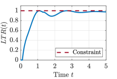
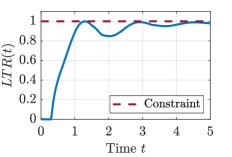
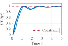
The rollover constraints are defined through the Load Transfer Ratio (LTR), and are imposed as , where for the given longitudinal speed is .
We use YALMIP toolbox [69] to implement the computations of the conventional CG scheme. The worst-case execution time for the conventional CG from 2000 runs is 200 ms. Thus, the sampling period of the conventional CG should be ms.
5.2 System Performance—Comparison Study
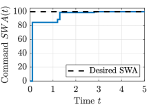
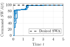
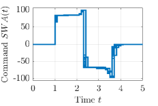
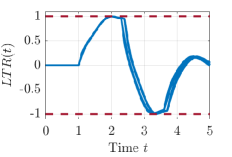
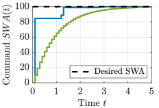
We consider the following three cases: Case I) There is no computational limitation (for instance, we implement the tasks on a more powerful processor), and we implement the conventional CG every 100 milliseconds; Case II) We implement the conventional CG, and to satisfy the real-time schedulability condition (7), we let the sampling period of the second task to be 300 [ms]; and Case III) We set the sampling period of the second task to 100 [ms], and implement ROTEC with , , and . For comparison purposes, we define the performance index as , where the integration is performed over the duration of the simulations.
Simulation results are shown in Figure 4, where 2000 runs are presented for Case III. The normalized achieved PIs for all cases are reported in TABLE 1, where the achieved PI for Case I is used as the basis for normalization. As seen in this table, using a large sampling period (Case II) can degrade the performance. ROTEC (Case III) yields a better performance by computing a sub-optimal solution every 100 ms.
(a)

(b)
(c)
| Case I | Case II | Case III | |
|---|---|---|---|
| Normalized PI | 1 | 1.82 | 1.34 (Mean) |
5.3 Rollover Prevention—Fishhook Test
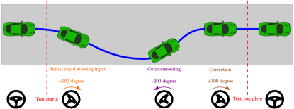
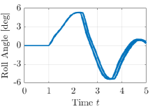
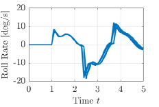
To investigate the constraint-handling property of ROTEC, we conduct the fishhook test [70, 71]. This test is a steer/countersteer maneuver, in which to achieve the maximum severity, the desired SWA switches when the maximum roll angle is reached. This test is described in Figure 5.
Simulation results are shown in Figure 6. As seen in this figure, ROTEC ensures that the vehicle will not roll over when subject to a severe obstacle avoidance maneuver.
5.4 Impact of A High Number of Early Terminations
In this subsection, we study the impact of a high number of early terminations on the performance of ROTEC. To conduct this study, we discretize the vehicle dynamics with a sampling period of 100 msec, but we limit the execution time of ROTEC to 10 sec. Such a limitation ensures that the CG task faces early termination at most of the sampling instants. A high number of early terminations prevents ROTEC from converging to the optimal solution at most of the sampling instants. As seen from Figure 7, this degrades the tracking performance and slows down the convergence of the CG output to the reference command. Nevertheless, the constraints are not violated and convergence of CG output to the reference command is still achieved.
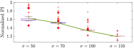
5.5 Sensitivity Analysis—Impact of
We conducted sensitivity analysis of the performance of ROTEC with respect to the design parameter . Figure 8 shows how impacts the performance. From Figure 8 we see that as decreases, the performance of ROTEC degrades. This is consistent with expectations from (29). Note that a large also reduces the number of discarded as a result of violation of (37), such that the mean number of rejected command signals is and for and , respectively.


5.6 Sensitivity Analysis—Impact of Sampling Period
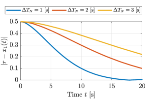
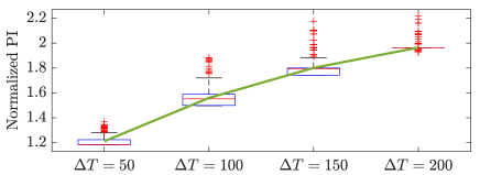
In this subsection, we study the sensitivity of ROTEC to the sampling period. For this study, we assume that the vehicle dynamics are discretized with different sampling periods, and ROTEC is the only control system running on the processor. Figure 9 shows how sampling period impacts the performance of closed-loop system. As discussed in Section 2, the larger the sampling period is, the poorer performance of the CG scheme could become. This is illustrated in Figure 9.
6 Conclusion
This paper proposed ROTEC (RObust to early TErmination Command governor), an algorithm capable of maintaining feasibility of command governor by adapting to available computation times. Variability in time available to perform computations is a common occurrence in modern Cyber-Physical Systems, where several tasks can run on the same processor. The core idea of ROTEC is to use a continuous-time primal-dual gradient flow algorithm that is run for as long as the processor is available for computation, and to augment such an algorithm with an acceptance/rejection logic. ROTEC guarantees constraint satisfaction at all times, and provides a sub-optimal but feasible and effective solution if early terminated due to limited computation time. The effectiveness of ROTEC is validated through simulation studies of vehicle rollover prevention. The paper shows that ROTEC addresses the availability of limited computating power, yields an acceptable performance, and guarantees rollover prevention under severe steer/countersteer maneuvers.
Future research will consider how other optimization-based controllers can be implemented in a way that is robust to early termination and variability in available processor power.
References
- [1] C. Liu and J. Layland, “Scheduling algorithms for multiprogramming in a hard real-time environment,” Journal of the ACM, vol. 20, no. 1, pp. 46–61, 1973.
- [2] G. Buttazzo, Hard Real-Time Computing Systems: Predictable Scheduling Algorithms and Applications. Springer US, 2011.
- [3] M. Dertouzos, “Control robotics : the procedural control of physical processors,” in Proceedings of the IFIP Congress, 1974, pp. 807–813.
- [4] M. Short, “Improved schedulability analysis of implicit deadline tasks under limited preemption EDF scheduling,” in Proc. Int. Conf. Emerging Technologies and Factory Automation, Toulouse, France, Sep. 5–9, 2011.
- [5] E. Bini and A. Cervin, “Delay-aware period assignment in control systems,” in Proc. 2008 Real-Time Systems Symposium, Barcelona, Spain, Nov. 30–Dec. 3, 2008, pp. 291–300.
- [6] D. Roy, C. Hobbs, J. H. Anderson, M. Caccamo, and S. Chakraborty, “Timing debugging for cyber—physical systems,” in Proc. 2021 Design, Automation and Test in Europe Conference and Exhibition, Grenoble, France, Feb. 1–5, 2021, pp. 1893–1898.
- [7] R. Wilhelm, J. Engblom, A. Ermedahl, N. Holsti, S. Thesing, D. Whalley, G. Bernat, C. Ferdinand, R. Heckmann, T. Mitra, F. Mueller, I. Puaut, P. Puschner, J. Staschulat, and P. Stenstrom., “The worst-case execution-time problem—overview of methods and survey of tools,” ACM Transactions on Embedded Computing Systems, vol. 7, no. 3, pp. 36–53, Apr. 2008.
- [8] C. Lozoya, P. Martí, M. Velasco, J. M. Fuertes, and E. X. Martin, “Resource and performance trade-offs in real-time embedded control systems,” Real-Time Systems, vol. 49, pp. 267–307, 2013.
- [9] L. Palopoli, C. Pinello, A. Bicchi, and A. Sangiovanni-Vincentelli, “Maximizing the stability radius of a set of systems under real-time scheduling constraints,” IEEE Transactions on Automatic Control, vol. 50, no. 1, pp. 1790–1795, Nov. 2005.
- [10] M. Velasco, P. Martí, J. M. Fuertes, C. Lozoya, and S. A.Brandt, “Experimental evaluation of slack management in real-time control systems: Coordinated vs. self-triggered approach,” Journal of Systems Architecture, vol. 56, no. 1, pp. 63–74, 2010.
- [11] W. Chang, D. Goswami, S. Chakraborty, and A. Hamann, “OS-aware automotive controller design using non-uniform sampling,” ACM Transactions on Cyber-Physical Systems, vol. 2, no. 4, Sep. 2018.
- [12] H. S. Chwa, K. G. Shin, and J. Lee, “Closing the gap between stability and schedulability: A new task model for cyber-physical systems,” in Proc. IEEE Real-Time and Embedded Technology and Applications Symposium, Porto, Portugal, Apr. 11–13, 2018, pp. 327–337.
- [13] W. Chang, D. Goswami, S. Chakraborty, L. Ju, C. J. Xue, and S. Andalam, “Memory-aware embedded control systems design,” IEEE Transactions on Computer-Aided Design of Integrated Circuits and Systems, vol. 36, no. 4, pp. 586–599, Apr. 2017.
- [14] P. Pazzaglia, A. Hamann, D. Ziegenbein, and M. Maggio, “Adaptive design of real-time control systems subject to sporadic overruns,” in Proc. 2021 Design, Automation and Test in Europe Conference and Exhibition, Grenoble, France, Feb. 1–5, 2021, pp. 1887–1892.
- [15] N. Vreman, A. Cervin, and M. Maggio, “Stability and performance analysis of control systems subject to bursts of deadline misses,” in Proc. 33rd Euromicro Conference on Real-Time Systems, Jul. 5–9, 2021.
- [16] G. Buttazzo, M. Velasco, P. Marti, and G. Fohler, “Managing quality-of-control performance under overload conditions,” in Proc. 16th Euromicro Conf. Real-Time Systems, Catania, Italy, Jul. 2, 2004.
- [17] P. Tabuada, “Event-triggered real-time scheduling of stabilizing control tasks,” IEEE Transactions on Automatic Control, vol. 52, no. 9, pp. 1680–1685, Sep. 2007.
- [18] M. Ryu, H. S, and M. Saksena, “Streamlining real-time controller design: From performance specifications to end-to-end timing constraints,” in Proc. 3rd IEEE Real-Time Technology and Applications Symposium, Montreal, QC, Canada, Jun. 9–11, 1997, pp. 91–99.
- [19] A. Aminifar, E. Bini, P. Eles, and Z. Peng, “Analysis and design of real-time servers for control applications,” IEEE Transactions on Computers, vol. 65, no. 3, pp. 834–846, Mar. 2016.
- [20] V. P. Kumar and A. S. Pillai, “Dynamic scheduling algorithm for a utomotive safety critical systems,” in Proc. 4th Int. Conf. Computing Methodologies and Communication, Erode, India, Mar. 11–13, 2020, pp. 815–820.
- [21] P. Fara, G. Serra, A. Biondi, and C. Donnarumma, “Scheduling replica voting in fixed-priority real-time systems,” in Proc. 33rd Euromicro Conf. Real-Time Systems, Modena, Italy, Jul. 5–8, 2021.
- [22] Y. Zhao and H. Zeng, “The virtual deadline based optimization algorithm for priority assignment in fixed-priority scheduling,” in Proc. IEEE Real-Time Systems Symposium, Paris, France, Dec. 5–8, 2017, pp. 116–127.
- [23] Y. Lin, X. Jin, T. Zhang, M. Han, N. Guan, and Q. Deng, “Queue assignment for fixed-priority real-time flows in time-sensitive networks: Hardness and algorithm,” Journal of Systems Architecture, vol. 116, 2021.
- [24] E. F. Camacho and C. B. Alba, Model Predictive Control, 2nd ed. Springer-Verlag London, 2007.
- [25] J. B. Rawlings, D. Q. Mayne, and M. M. Diehl, Model Predictive Control: Theory, Computation, and Design, 2nd ed. Nob Hill Publishing, LLC, 2017.
- [26] E. Garone, I. Kolmanovsky, and S. D. Cairano, “Reference and command governors for systems with constraints: a survey on theory and applications,” Automatica, vol. 75, pp. 306–328, Jan. 2016.
- [27] A. D. Ames, S. Coogan, M. Egerstedt, G. Notomista, K. Sreenath, and P. Tabuada, “Control barrier functions: Theory and applications,” in Proc. 18th European Control Conference, Naples, Italy, Jun. 25–28, 2019, pp. 3420–3431.
- [28] A. Alessio and A. Bemporad, “A survey on explicit model predictive control,” in Nonlinear model predictive control: Towards new challenging applications, L. Magni, D. M. Raimondo, and F. Allgower, Eds. Springer Berlin Heidelberg, 2009, pp. 345–369.
- [29] E. Henriksson, D. E. Quevedo, H. Sandberg, and K. H. Johansson, “Self-triggered model predictive control for network scheduling and control,” in Proc. 8th IFAC Symposium on Advanced Control of Chemical Processes, Singapore, Jul. 10–13, 2012, pp. 432–438.
- [30] J. Yoo and K. H. Johansson, “Event-triggered model predictive control with a statistical learning,” IEEE Transactions on Systems, Man, and Cybernetics: Systems, vol. 51, no. 4, pp. 2571–2581, Apr. 2021.
- [31] B. Wang, J. Huang, C. Wen, J. Rodriguez, C. Garcia, H. B. Gooi, and Z. Zeng, “Event-triggered model predictive control for power converters,” IEEE Transactions on Industrial Electronics, vol. 68, no. 1, pp. 715–720, Jan. 2021.
- [32] R. Ghaemi, J. Sun, and I. V. Kolmanovsky, “An integrated perturbation analysis and sequential quadratic programming approach for model predictive control,” Automatica, vol. 45, no. 10, pp. 2412–2418, Oct. 2009.
- [33] D. Liao-McPherson, M. M. Nicotra, and I. Kolmanovsky, “Time-distributed optimization for real-time model predictive control: Stability, robustness, and constraint satisfaction,” Automatica, vol. 117, Jul. 2020.
- [34] G. Cimini and A. Bemporad, “Exact complexity certification of active-set methods for quadratic programming,” IEEE Transactions on Automatic Control, vol. 62, no. 12, pp. 6094–6109, Dec. 2017.
- [35] M. M. Nicotra, D. Liao-McPherson, and I. V. Kolmanovsky, “Dynamically embedded model predictive control,” in Proc. 2018 Annual American Control Conference, Milwaukee, WI, USA, Jun. 27–29, 2018, pp. 4957–4962.
- [36] Y. Wang and S. Boyd, “Fast model predictive control using online optimization,” IEEE Transactions on Control Systems Technology, vol. 18, no. 2, pp. 267–278, Mar. 2010.
- [37] M. M. Nicotra, D. Liao-McPherson, and I. V. Kolmanovsky, “Embedding constrained model predictive control in a continuous-time dynamic feedback,” IEEE Transactions on Automatic Control, vol. 64, no. 5, pp. 1932–1946, May 2019.
- [38] E. Hermand, T. W. Nguyen, M. Hosseinzadeh, and E. Garone, “Constrained control of UAVs in geofencing applications,” in Proc. 26th Mediterranean Conf. Control and Automation, Zadar, Croatia, Jun. 19–22, 2018, pp. 217–222.
- [39] A. Cotorruelo, M. Hosseinzadeh, D. R. Ramirez, D. Limon, and E. Garone, “Reference dependent invariant sets: Sum of squares based computation and applications in constrained control,” Automatica, vol. 129, Jul. 2021.
- [40] M. Hosseinzadeh, K. van Heusden, G. A. Dumont, and E. Garone, “An explicit reference governor scheme for closed-loop anesthesia,” in Proc. 18th European Control Conference, Naples, Italy, Jun. 25–28, 2019, pp. 1294–1299.
- [41] D. Famularo, G. Franzè, A. Furfaro, and M. Mattei, “A hybrid real-time command governor supervisory scheme for constrained control systems,” IEEE Transactions on Control Systems Technology, vol. 23, no. 3, pp. 924–936, May 2015.
- [42] Z. Peng, J. Wang, and J. Wang, “Constrained control of autonomous underwater vehicles based on command optimization and disturbance estimation,” IEEE Transactions on Industrial Electronics, vol. 66, no. 5, pp. 3627–3635, May 2019.
- [43] M. Hosseinzadeh and E. Garone, “An explicit reference governor for the intersection of concave constraints,” IEEE Transactions on Automatic Control, vol. 65, no. 1, pp. 1–11, Jan. 2020.
- [44] M. Hosseinzadeh, E. Garone, and L. Schenato, “A distributed method for linear programming problems with box constraints and time-varying inequalities,” IEEE Control Systems Letters, vol. 3, no. 2, pp. 404–409, Apr. 2019.
- [45] M. Hosseinzadeh, A. Cotorruelo, D. Limon, and E. Garone, “Constrained control of linear systems subject to combinations of intersections and unions of concave constraints,” IEEE Control Systems Letters, vol. 3, no. 3, pp. 571–576, Jul. 2019.
- [46] T. A. Henzinger, B. Horowitz, and C. M. Kirsch, “Giotto: a time-triggered language for embedded programming,” Proceedings of the IEEE, vol. 91, no. 1, pp. 84–99, Jan. 2003.
- [47] G. Frehse, A. Hamann, S. Quinton, and M. Woehrle, “Formal analysis of timing effects on closed-loop properties of control software,” in Proc. IEEE Real-Time Systems Symposium, Rome, Italy, Dec. 2–5, 2014, pp. 53–62.
- [48] H. Liang, Z. Wang, D. Roy, S. Dey, S. Chakraborty, and Q. Zhu, “Security-driven codesign with weakly-hard constraints for real-time embedded systems,” in Proc. 37th Int. Conf. Computer Design, Abu Dhabi, United Arab Emirates, Nov. 17–20, 2019, pp. 217–226.
- [49] K. Ogata, Discrete-Time Control Systems, 2nd ed. Pearson, 1995.
- [50] R. E. Kalman, Y. E. Ho, and K. S. Narendra, “Controllability of linear dynamical systems,” Contribution to Differential Equations, vol. 1, pp. 189–213, 1962.
- [51] S. M. Karbassi and D. J. Bell, “The effect of sampling period on the behaviour of systems incorporating state feedback,” International Journal of Control, vol. 63, no. 2, pp. 351–364, 1996.
- [52] A. Bemporad, C. Filippi, and F. D. Torrisi, “Inner and outer approximations of polytopes using boxes,” Computational Geometry, vol. 27, no. 2, pp. 151–178, Feb. 2004.
- [53] E. G. Gilbert and K. T. Tan, “Linear systems with state and control constraints: the theory and application of maximal output admissible sets,” IEEE Transactions on Automatic Control, vol. 36, no. 9, pp. 1008–1020, Sep. 1991.
- [54] S. Boyd and L. Vandenberghe, Convex Optimization. Cambridge University Press, 2004.
- [55] R. Polyak, “Modified barrier functions (theory and methods),” Mathematical Programming, vol. 54, no. 1–3, pp. 177–222, Feb. 1992.
- [56] K. Ryu and S. Boyd, “Primer on monotone operator methods,” Appl. Comput. Math, vol. 15, no. 1, pp. 3–43, Jan. 2016.
- [57] M. Fazlyab, S. Paternain, V. M. Preciado, and A. Ribeiro, “Interior point method for dynamic constrained optimization in continuous time,” in Proc. 2016 American Control Conference, Boston, MA, USA, Jul. 6–8, 2016, pp. 5612–5618.
- [58] M. Gilli, D. Maringer, and E. Schumann, Numerical Methods and Optimization in Finance, 2nd ed. Academic Press, 2019.
- [59] A. D. Alexandrov, Convex Polyhedra. Springer-Verlag Berlin Heidelberg, 2005.
- [60] E. Garone and I. Kolmanovsky, “Command governors with inexact optimization and without invariance,” arXiv:2111.10234, 2021, https://arxiv.org/abs/2111.10234.
- [61] M. Ataei, A. Khajepour, and S. Jeon, “Model predictive control for integrated lateral stability, traction/braking control, and rollover prevention of electric vehicles,” Vehicle System Dynamics, vol. 58, no. 1, pp. 49–73, 2020.
- [62] Y. Shi, Y. Huang, and Y. Chen, “Trajectory planning of autonomous trucks for collision avoidance with rollover prevention,” IEEE Transactions on Intelligent Transportation Systems, 2021.
- [63] M. Ibrahim, C. Kallies, and R. Findeisen, “Learning-supported approximated optimal control for autonomous vehicles in the presence of state dependent uncertainties,” in Proc. European Control Conference, St. Petersburg, Russia, May 12–15, 2020, pp. 338–343.
- [64] S. W. Kim, K. Ko, H. Ko, and V. C. M. Leung, “Edge-network-assisted real-time object detection framework for autonomous driving,” IEEE Network, vol. 35, no. 1, pp. 177–183, Jan./Feb. 2021.
- [65] F. E. Ophelders, S. Chakraborty, and H. Corporaal, “Intra- and inter-processor hybrid performance modeling for mpsoc architectures,” in Proc. 6th IEEE/ACM/IFIP int. conf. Hardware/Software codesign and system synthesis, Atlanta, GA, USA, Oct. 19–24, 2008, pp. 91–96.
- [66] Y. Lu, T. Nolte, I. Bate, and L. Cucu-Grosjean, “A statistical response-time analysis of real-time embedded systems,” in Proc. IEEE 33rd Real-Time Systems Symposium, San Juan, PR, USA, Dec. 4–7, 2012, pp. 351–362.
- [67] R. Bencatel, R. Tian, A. R. Girard, and I. Kolmanovsky, “Reference governor strategies for vehicle rollover avoidance,” IEEE Transactions on Control Systems Technology, vol. 26, no. 6, pp. 1954–1969, Nov. 2019.
- [68] K. Liu, N. Li, I. Kolmanovsky, D. Rizzo, and A. Girard, “Model-free learning for safety-critical control systems: A reference governor approach,” in Proc. American Control Conference, Denver, CO, USA, Jul. 1–3, 2020, pp. 943–949.
- [69] J. Lofberg, “YALMIP: a toolbox for modeling and optimization in MATLAB,” in Proc. IEEE Int. Conf. Robotics and Automation, Taipei, Taiwan, Sep. 2–4, 2004, pp. 284–289.
- [70] H. Dahmani, O. Pages, and A. E. Hajjaji, “Observer-based state feedback control for vehicle chassis stability in critical situations,” IEEE Transactions on Control Systems Technology, vol. 24, no. 2, pp. 636–643, Mar. 2016.
- [71] M. Mehrtash, T. Yuen, and L. Balan, “Implementation of experiential learning for vehicle dynamic in automotive engineering: Roll-over and fishhook test,” Procedia Manufacturing, vol. 32, pp. 768–774, 2019.
Appendix
Lemma.
Let , and , be given vectors and real numbers, respectively. Suppose that it is known that for some . Let
and assume that
| (Condition ) |
Let
Then, there exists such that for all satisfying the above assumptions the value of admits the following bound:
Proof.
Since , one can rewrite as
Since and is a closed set, there is a minimum distance between and the set . Thus, letting completes the proof. ∎