Time-dependent exchange-correlation potential in lieu of self-energy

Abstract

It is shown that the equation of motion of the one-particle Green function of an interacting many-electron system is governed by a multiplicative time-dependent exchange-correlation potential, which is the Coulomb potential of a time-dependent exchange-correlation hole. This exchange-correlation hole fulfills a sum rule, a generalization of the well-known sum rule of the static exchange-correlation hole. It is envisaged that the proposed formalism may provide an alternative route for calculating the Green function by finding a suitable approximation for the exchange-correlation hole or potential based on, e.g., a local-density approximation.

I Introduction

The one-particle Green function of an interacting many-particle system is of utmost importance in condensed-matter physics and other branches of physics such as molecular physics and nuclear physics. Essential physical properties, notably the ground-state expectation value of a single-particle operator, the total energy, and the particle addition and removal spectra can be extracted from the one-particle Green function, hereafter referred to simply as the Green function. Experimental photoemission and inverse photoemission spectra, which provide invaluable information about the electronic structure of the system, can be directly compared with the spectra extracted from the Green function, under the so-called sudden approximation and neglecting the matrix-element effects. Experimental data from transport measurements and many other experimental observations can also be related to the Green function. A lot of efforts have therefore been expended on developing methods and techniques for calculating the Green function, from many-body perturbation theory fetter-walecka to methods employing path-integral techniques negele .

The zero-temperature time-ordered Green function is defined according to fetter-walecka

$$iG(rt,r^{\prime}t^{\prime})=\langle T[\hat{\psi}(rt\mathbf{)}\hat{\psi}^{{\dagger}}(r^{\prime}t^{\prime})]\rangle,$$ (1)

where $r=(\mathbf{r,}\sigma)$ is a combined label of space and spin variables, $\hat{\psi}(rt\mathbf{)}$ is the field operator in the Heisenberg picture, $T$ is the time-ordering symbol, and the expectation value is taken with respect to the ground-state. The many-electron Hamiltonian defining the Heisenberg operator is given by

$$\hat{H} =\int dr\text{ }\hat{\psi}^{{\dagger}}(r)h_{0}(r)\hat{\psi}(r)$$

$$+\frac{1}{2}\int drdr^{\prime}\text{ }\hat{\psi}^{{\dagger}}(r)\hat{\psi}^{{\dagger}}(r^{\prime})v(r-r^{\prime})\hat{\psi}(r^{\prime})\hat{\psi}(r),$$ (2)

where $h_{0}=-\frac{1}{2}\nabla^{2}+V_{ext}(r)$ and $v(r-r^{\prime})=1/|\mathbf{r-r}^{\prime}|$. In our notation, $\int dr=\sum_{\sigma}\int d^{3}r$ and atomic unit is used throughout, in which the Bohr radius $a_{0}$, the electron mass $m_{e}$, the electronic charge $e$, and $\hbar$ are set to unity.

Since the Hamiltonian is time independent it is convenient to set $t^{\prime}=0$. The Green function fulfills the following equation of motion:

$$\left(i\frac{\partial}{\partial t}-h_{0}(r\mathbf{)}\right)G(r,r^{\prime};t)$$

$$+i\int dr^{\prime\prime}v(r-r^{\prime\prime})\langle T[\hat{\rho}(r^{\prime\prime}t)\hat{\psi}(rt\mathbf{)}\hat{\psi}^{{\dagger}}(r^{\prime})]\rangle$$

$$=\delta(r-r^{\prime})\delta(t).$$ (3)

where $\hat{\rho}$ is the density operator. The interaction term contains a special case of the two-particle Green function:

$$G^{(2)}(r,r^{\prime},r^{\prime\prime};t)=\langle T[\hat{\rho}(r^{\prime\prime}t)\hat{\psi}(rt\mathbf{)}\hat{\psi}^{{\dagger}}(r^{\prime})]\rangle.$$ (4)

The traditional approach is to introduce a self-energy $\Sigma$ as follows:

$$- i\int dr^{\prime\prime}v(r-r^{\prime\prime})G^{(2)}(r,r^{\prime},r^{\prime\prime};t)-V_{H}(r)G(r,r^{\prime};t)$$

$$=\int dr^{\prime\prime}dt^{\prime\prime}\Sigma(r,r^{\prime\prime};t-t^{\prime\prime})G(r^{\prime\prime},r^{\prime};t^{\prime\prime}),$$ (5)

where $V_{H}$ is the Hartree potential subtracted from $G^{(2)}$. Thus, the self-energy embodies the effects of exchange and correlations and a central quantity in Green function theory. The self-energy is a well-established framework for calculating the Green function but it acts on the Green function as a convolution in space and time and as such it is difficult to visualize its meaning in a clear physical picture. Moreover, from the Dyson equation, $G=G_{0}+G_{0}\Sigma G$, it can be seen that $\Sigma$ is an auxiliary quantity since it depends on the choice of the starting reference Green function $G_{0}$.

In this paper, a completely different route is proposed to calculate the Green function. It is shown that the equation of motion of the Green function can be reformulated so that it is governed by a time-dependent exchange-correlation potential that acts multiplicatively on the Green function. This exchange-correlation potential arises naturally from the Coulomb potential of the time-dependent exchange correlation hole, which fulfills a sum rule. The static and equal-space limit $r^{\prime}\rightarrow r$ of this exchange-correlation hole reduces to the well-known static exchange-correlation hole in the formal expression for the exchange-correlation energy. The focus is then shifted to finding an accurate approximation for the exchange-correlation hole or potential, in the spirit of density functional theory hohenberg1964 ; kohn1965 ; jones1989 ; becke2014 .

II Theory

II.1 Time-dependent exchange-correlation hole

Writing out the time ordering of the two-particle Green function in Eq. (4) and using the commutation

$$[\hat{\psi}(rt),\hat{\rho}(r^{\prime\prime}t)]=\delta(r-r^{\prime\prime})\hat{\psi}(rt).$$ (6)

yields

$$G^{(2)}(r,r^{\prime},r^{\prime\prime};t)=\langle\hat{\rho}(r^{\prime\prime}t)\hat{\psi}(rt)\hat{\psi}^{{\dagger}}(r^{\prime})\rangle\theta(t)$$

$$\text{ \ \ \ \ \ \ \ \ \ \ \ \ \ \ \ \ \ \ \ }-\langle\hat{\psi}^{{\dagger}}(r^{\prime})\hat{\psi}(rt)\hat{\rho}(r^{\prime\prime}t)\rangle\theta(-t)$$

$$\text{ \ \ \ \ \ \ \ \ \ \ \ \ \ \ }+\delta(r-r^{\prime\prime})\langle\hat{\psi}^{{\dagger}}(r^{\prime})\hat{\psi}(rt)\rangle\theta(-t).$$ (7)

Consider now integrating $G^{(2)}$ over the variable $r^{\prime\prime}$. It should first be noted that for any state $\Psi$ containing $N$ electrons,

$$\int dr^{\prime\prime}\hat{\rho}(r^{\prime\prime})\left|\Psi\right\rangle=\hat{N}\left|\Psi\right\rangle=N\left|\Psi\right\rangle,$$ (8)

where $\hat{N}$ counts the number of electrons in the system. Using $G^{(2)}$ in Eq, (7) one finds for $t<0$

$$\int dr^{\prime\prime}G^{(2)}(r,r^{\prime},r^{\prime\prime};t)=iG(r,r^{\prime};t)\left(N-1\right).$$ (9)

$G^{(2)}$ can be naturally factorized as follows:

$$G^{(2)}(r,r^{\prime},r^{\prime\prime};t)=iG(r,r^{\prime};t)g(r,r^{\prime},r^{\prime\prime};t)\rho(r^{\prime\prime}),$$ (10)

which defines the correlation function $g(r,r^{\prime},r^{\prime\prime};t)$, and after substitution into Eq. (9) one arrives at the sum rule

$$\int dr^{\prime\prime}[g(r,r^{\prime},r^{\prime\prime};t)-1]\rho(r^{\prime\prime})=-1.$$ (11)

This sum rule is valid for any $r,r^{\prime}$, and $t<0$ and the integrand may be interpreted as the time-dependent exchange-correlation hole:

$$\rho_{xc}(r,r^{\prime},r^{\prime\prime};t)=[g(r,r^{\prime},r^{\prime\prime};t)-1]\rho(r^{\prime\prime}),$$ (12)

a generalization of the static exchange-correlation hole, first introduced by Slater for the exchange part slater1951 . Since $\rho_{xc}(r,r^{\prime},r^{\prime\prime};t)$ is in general complex, the sum rule implies that the imaginary part integrates to zero.

It is interesting to observe that for $t>0$ (addition of an electron), the exchange-correlation hole integrates to zero as can be seen from Eq. (7). This result may be understood by recognizing that the added electron is not part of the electron density that generates the Hartree potential so that there is no self-interaction corresponding to the last term of $G^{(2)}$ in Eq. (7). For $\sigma^{\prime\prime}\neq\sigma$, the exchange-correlation hole integrates to zero as may be seen from the presence of $\delta(r-r^{\prime\prime})=\delta(\mathbf{r-r}^{\prime})\delta_{\sigma\sigma^{\prime\prime}}$ in Eq. (7). If one were to decompose $\rho_{xc}$ into the exchange and the correlation holes, it is the exchange hole that would integrate to $-1$ whereas the correlation hole would integrate to zero. The sum rule can then be summarized as follows:

$$\int d^{3}r^{\prime\prime}\rho_{xc}(r,r^{\prime},r^{\prime\prime};t) =-\delta_{\sigma\sigma^{\prime\prime}}\theta(-t),$$ (13)

This sum rule may be viewed as the generalization of the well-known sum rule for the static exchange-correlation hole appearing in the formally exact expression for the exchange-correlation energy jones1989 ; becke2014 , originating from Slater’s sum rule for exchange hole only slater1951 . The static exchange-correlation hole corresponds to the limit $t\rightarrow 0^{-}$ and $r^{\prime}\rightarrow r.$

II.2 Time-dependent exchange-correlation potential

Rearranging Eq. (10) yields

$$G^{(2)}(r,r^{\prime},r^{\prime\prime};t)$$

$$=iG(r,r^{\prime};t)\rho(r^{\prime\prime})+iG(r,r^{\prime};t)\rho_{xc}(r,r^{\prime},r^{\prime\prime};t),$$ (14)

in which the first term on the right-hand side generates the Hartree term. When the above $G^{(2)}$ is substituted into the equation of motion of $G$ in Eq. (3), it generates the time-dependent exchange-correlation potential as a function of $r,r^{\prime}$ and $t$:

$$V_{xc}(r,r^{\prime};t)=\int dr^{\prime\prime}v(r-r^{\prime\prime})\rho_{xc}(r,r^{\prime},r^{\prime\prime};t),$$ (15)

acting on $G$ in a multiplicative fashion, in contrast to the self-energy which acts on $G$ as a convolution in space-time as in Eq. (5). The equation of motion of $G$ becomes

$$\left(i\frac{\partial}{\partial t}-h(r\mathbf{)}-V_{xc}(r,r^{\prime};t)\right)G(r,r^{\prime};t)=\delta(r-r^{\prime})\delta(t),$$ (16)

where $h=h_{0}+V_{H}$. This equation has a local character in the sense that the potential is multiplicative in both space and time. Apart from the source term on the right-hand side, for a given $r^{\prime}$ it is just like a one-particle time-dependent Schrödinger equation in the presence of a time-dependent field $V_{xc}$. The effects of exchange and correlations are now embodied in the time-dependent exchange-correlation potential $V_{xc}$, which is in general non-Hermitian. Eq. (16) furnishes us with a different picture from that of the conventional self-energy formulation and offers a simple physical interpretation for the propagation of an added electron or hole, which is governed by, in addition to the external field and the Hartree potential, the time-dependent exchange-correlation potential. This exchange-correlation potential is simply the Coulomb potential of the time-dependent exchange-correlation hole.

The corresponding Dyson-like equation for $G$ can be readily written down:

$$G(r,r^{\prime};t)=G_{H}(r,r^{\prime};t)$$

$$+\int dr^{\prime\prime}dt^{\prime}G_{H}(r,r^{\prime\prime};t-t^{\prime})V_{xc}(r^{\prime\prime},r^{\prime};t^{\prime})G(r^{\prime\prime},r^{\prime};t^{\prime}),$$ (17)

where $G_{H}$ is the Hartree Green function, and the relationship between $V_{xc}$ and $\Sigma$ in space-time is given by

$$V_{xc}(r,r^{\prime};t)G(r,r^{\prime};t)=\int dr^{\prime\prime}dt^{\prime}\Sigma(r,r^{\prime\prime};t-t^{\prime})G(r^{\prime\prime},r^{\prime};t^{\prime}).$$ (18)

Expressed in a set of base orbitals $\{\varphi_{i}\}$, the equation of motion in Eq. (16) takes the form

$$i\frac{\partial}{\partial t}G_{ij}(t)-\sum_{k}h_{ik}G_{kj}(t)-\sum_{kl}V_{ik,lj}^{xc}(t)G_{kl}(t)=\delta_{ij}\delta(t),$$ (19)

where $G_{ij}$ and $h_{ik}$ are the matrix elements of $G$ and $h$ in the orbitals and

$$V_{ik,lj}^{xc}(t)=\int d^{3}rd^{3}r^{\prime}\text{ }\varphi_{i}^{\ast}(r)\varphi_{k}(r)V_{xc}(r,r^{\prime};t)\varphi_{l}^{\ast}(r^{\prime})\varphi_{j}(r^{\prime}),$$ (20)

exhibiting the two-particle character of $V_{xc}$, a Bosonic quantity, in contrast to the self-energy which is Fermionic.

Much is known about the static exchange-correlation hole becke2014 , which may provide a starting point for finding a good approximation for the time-dependent one. Approximating $V_{xc}$ via the exchange-correlation hole $\rho_{xc}$, which is a physically motivated entity, may be more advantageous than following the arduous route of finding a good approximation for the self-energy by means of many-body perturbation theory or path integral approach. The proposed formalism has a certain proximity to time-dependent density functional theory runge1984 ; maitra2016 . It should be noted, however, that the time dependence of $V_{xc}$ does not arise from the presence of a time-dependent external field, but rather due to the dynamics of the Green function. The addition or removal of an electron causes the system to evolve in a non-trivial way due to the Coulomb interaction among the electrons.

II.3 Local-density approximation

It can be anticipated that $V_{xc}$ is a relatively smooth function since it is the Coulomb potential of a charge distribution that integrates to $-1$ or $0$. Following Gunnarsson and Lundqvist gunnarsson1976 ; jones1989 , it is readily seen by making a change of variable $\mathbf{R}=\mathbf{r}-\mathbf{r}^{\prime\prime}$ that, due to the form of the Coulomb interaction, only the spherical average of the exchange-correlation hole in the variable $\mathbf{R}$ is needed to determine $V_{xc}$:

$$V_{xc}(r,r^{\prime};t)=\sum_{\sigma_{R}}\int dRR\text{ }\overline{\rho}_{xc}(r,r^{\prime},R;t),$$ (21)

where $\overline{\rho}_{xc}(r,r^{\prime},R;t)$ depends only on the radial distance $R$ with respect to $\mathbf{r}$,

$$\overline{\rho}_{xc}(r,r^{\prime},R;t)=\int d\Omega_{R}\rho_{xc}(r,r^{\prime},\mathbf{r-R};t),$$ (22)

implying that the fine spatial details of the exchange-correlation hole may not be important as illustrated vividly for the case of the static exchange-correlation hole in some light atoms gunnarsson1979 ; jones1989 . According to Eq. (21), $V_{xc}$ is the first radial moment of the spherically averaged $\rho_{xc}$.

It can also be seen that $\mathbf{r}$ may be thought of as the center of the exchange-correlation hole whereas $r^{\prime}$ may be treated as a parameter representing the spatial origin of the created electron. One could imagine that the exchange-correlation hole moves with the added hole or electron as a function of time. From Eq. (7) it is quite evident that when $r^{\prime\prime}=r$, $G^{(2)}=g=0$ and hence

$$\rho_{xc}(r,r^{\prime},r;t)=-\rho(r)$$ (23)

for any $r,$ $r^{\prime},$ and $t$. Following Slater’s argument slater1968 , it can be concluded that the exchange-correlation potential behaves approximately as $\rho^{1/3}$. It may be envisaged that a local-density approximation for $V_{xc}$ as in density functional theory can be developed and its time-dependence can be constructed from knowledge of the time-dependent exchange-correlation hole of the electron gas and some generic model systems, depending on the correlation strength.

The correlation function of the homogeneous electron gas with density $\bar{\rho}$ can be written as follows:

$$g^{HEG}_{\sigma\sigma^{\prime\prime}}(\bar{\rho},R^{\prime},R^{\prime\prime},\theta;t),$$ (24)

where $R^{\prime}=|\mathbf{r-r^{\prime}}|$, $R^{\prime\prime}=|\mathbf{r-r^{\prime\prime}}|$, $\theta$ is the angle between $\mathbf{R}^{\prime}$ and $\mathbf{R}^{\prime\prime}$, and the spin dependence has been written explicitly. A simple local-density approximation for the exchange-correlation hole could be

$$\rho_{xc}^{LDA}(r,r^{\prime},r^{\prime\prime};t)$$

$$=\left[g^{HEG}_{\sigma\sigma^{\prime\prime}}(\rho(r),R^{\prime},R^{\prime\prime},\theta;t)-1\right]\rho(r^{\prime\prime}).$$ (25)

A more sophisticated approximation would be to employ the weighted-density approximation alonso1978 ; gunnarsson1979 , in which the density dependence associated with the variable $r^{\prime}$ is taken into account. On the other hand, applying the local-density approximation directly on $V_{xc}$,

$$V_{xc}^{LDA}(r,r^{\prime};t)=V_{xc}^{HEG}(\rho(r),R;t),$$ (26)

where $R=|\mathbf{r-r^{\prime}}|$, may be too crude since information encoded in $\rho(r^{\prime\prime})$ is lost. It would be interesting to compare this approximation with the local-density approximation for the self-energy based on the homogeneous electron gas proposed by Sham and Kohn many years ago sham1966 . One may speculate that a local-density approximation on $V_{xc}$ is more favorable than on $\Sigma$ since $V_{xc}$ acts locally on $G$. Also, in contrast to $\Sigma$, which is Fermionic, $V_{xc}$ is a Bosonic object and as such it may be easier to approximate in terms of the density, which is a Bosonic quantity.

II.4 Connection with Kohn-Sham $V_{xc}$

If $V_{xc}(r,r^{\prime};t)$ is approximated by the static Kohn-Sham exchange-correlation potential, $V^{KS}_{xc}(r)$, then the Green function reduces to the Kohn-Sham non-interacting Green function, whose diagonal component will by construction yield the exact density. However, $V^{KS}_{xc}(r)$ is not necessarily the same as $V_{xc}(r,r;0^{-})$. From the equations of motion of $G$ and $G^{KS}$ one finds

$$\left(i\frac{\partial}{\partial t}-h(r\mathbf{)}-V_{xc}(r,r^{\prime};t)\right)[G(r,r^{\prime};t)-G^{KS}(r,r^{\prime};t)]$$

$$=[V_{xc}(r,r^{\prime};t)-V^{KS}_{xc}(r)]G^{KS}(r,r^{\prime};t).$$ (27)

Evaluating the equation at $r^{\prime}\rightarrow r$ and $t\rightarrow 0^{-}$ and making use of the fact that both $G$ and $G^{KS}$ give the same density yields the relationship between $V_{xc}(r,r;0^{-})$ and $V^{KS}_{xc}(r)$:

$$\lim_{r^{\prime}\rightarrow r,t\rightarrow 0^{-}}\left(\frac{\partial}{\partial t}-\frac{i}{2}\nabla^{2}\right)[G(r,r^{\prime};t)-G^{KS}(r,r^{\prime};t)]$$

$$=[V_{xc}(r,r;0^{-})-V^{KS}_{xc}(r)]\rho(r).$$ (28)

There is no obvious reason that the left-hand side vanishes so that in general $V_{xc}(r,r;0^{-})\neq V^{KS}_{xc}(r)$. When integrated over $r$, the first term on the left-hand side involving time derivative is the difference in the first moment of the occupied densities of states, whereas the second term is the difference in the kinetic energies, which is contained in the Kohn-Sham $E_{xc}$.

One also notes that

$$g(r,r,r^{\prime\prime};t=0^{-})\neq g^{KS}(r,r^{\prime\prime}),$$ (29)

since $g^{KS}$ is defined as a coupling-constant integration of $g_{\lambda}$, which is the static correlation function corresponding to a scaled Coulomb interaction, $\lambda v$, yielding the exact ground-state density independent of $\lambda$ gunnarsson1976 ; perdew1975 .

The exchange-correlation energy in the Kohn-Sham scheme is given by

$$E^{KS}_{xc}=\frac{1}{2}\int drdr^{\prime}\rho(r)v(r-r^{\prime})\rho_{xc}^{KS}(r,r^{\prime}),$$ (30)

where

$$\rho_{xc}^{KS}(r,r^{\prime})=[g^{KS}(r,r^{\prime})-1]\rho(r^{\prime})$$ (31)

is the static Kohn-Sham exchange-correlation hole. It can then be seen that the Kohn-Sham exchange-correlation potential is given by

$$V^{KS}_{xc}(r) =\int dr^{\prime}v(r-r^{\prime})\rho_{xc}^{KS}(r,r^{\prime})$$

$$+\frac{1}{2}\int dr^{\prime}dr^{\prime\prime}\rho(r^{\prime})v(r^{\prime}-r^{\prime\prime})\frac{\delta g^{KS}(r^{\prime},r^{\prime\prime})}{\delta\rho(r)}\rho(r^{\prime\prime}).$$ (32)

Thus in addition to the Coulomb potential of the exchange-correlation hole, which is the counterpart of $V_{xc}$ in Eq. (15), there is an additional contribution arising from the dependence of the distribution function $g^{KS}$ on the density.

II.5 Kohn-Sham scheme for unoccupied states

Since $V_{xc}(0^{-})\neq V_{xc}(0^{+})$, there will in general be a discontinuity at $t=0$. This suggests that in the Kohn-Sham scheme, two exchange-correlation potentials are needed, one for the occupied states and another for the unoccupied ones. For the occupied states, the standard Kohn-Sham equation applies while for the unoccupied states one has

$$\left(-\frac{1}{2}\nabla^{2}+V_{ext}+V_{H}+V^{+}_{xc}\right)\phi_{kn}=\epsilon_{k}\phi_{kn},$$ (33)

where $V^{+}_{xc}$ is the exchange-correlation potential corresponding to an exchange-correlation hole that integrates to zero rather than to one. After solving the standard Kohn-Sham equation, the unoccupied states are used to diagonalize Eq. (33), which ensures that all states will be orthogonal. A local density approximation for the exchange-correlation hole corresponding to $V^{+}_{xc}$ can be taken to be the one in Eq. (25) with $r^{\prime}=r$ and $t=0^{+}$.

Since the exchange-correlation hole corresponding to $V^{+}_{xc}$ integrates to zero, it should be weaker than the one for the occupied states for weakly or moderately correlated systems. This implies that the unoccupied states would be pushed up, correcting the well-known underestimation of band gaps in semiconductors and insulators. For metals, however, one may reason that since the band dispersion is smooth across the Fermi surface, the discontinuity should tend to vanish.

As an approximate $V^{+}_{xc}$ it may be reasonable to use only the correlation part of the standard $V_{xc}$. A simple correction would be to use first-order perturbation theory:

$$\varepsilon_{kn}^{+}=\varepsilon_{kn}+\langle\phi_{kn}|V^{+}_{xc}-V_{xc}|\phi_{kn}\rangle.$$ (34)

An even simpler correction would be to ignore entirely $V^{+}_{xc}$, which may lead, however, to an overestimation of the gap since $V^{+}_{xc}$ is likely to be negative.

II.6 Extension to temperature-dependent Green function

The temperature-dependent Green function is defined in a similar way as for the zero-temperature one with the ground-state expectation value replaced by the thermal average:

$$iG_{\beta}(rt,r^{\prime}t^{\prime}) =\frac{1}{Z}\mathrm{Tr}\left\{e^{-\beta\hat{K}}T[\hat{\psi}(rt)\hat{\psi}^{\dagger}(r^{\prime}t^{\prime})]\right\},$$ (35)

where $\hat{K}=\hat{H}-\mu\hat{N}$, $\mu$ is the chemical potential, $Z=\mathrm{Tr}\>e^{-\beta\hat{K}}$ is the partition function, and $\beta=1/(k_{B}T)$ with $k_{B}$ being the Boltzmann constant and $T$ the temperature. The Heisenberg operators is defined as

$$\hat{\psi}(rt)=e^{i\hat{K}t}\hat{\psi}(r)e^{-i\hat{K}t}.$$ (36)

At this stage, one traditionally goes over to imaginary time yielding the Matsubara Green function. The reason is that Wick’s theorem is no longer convenient to use if one stays along the real-time axis due to the presence of the thermal factor $e^{-\beta\hat{K}}$. The proposed formalism, however, makes no use of Wick’s theorem so that it is not necessary to work along the imaginary-time axis. The ill-defined problem of analytic continuation to the real-time axis when calculating spectral functions associated with the Matsubara Green function is circumvented.

The field operators are independent of temperature so that the equation of motion of $G_{\beta}$ is the same as the one in Eq. (3) with the understanding that ground-state expectation value is now to be understood as thermal average and $h_{0}$ is replaced with $h_{0}-\mu$. It is quite evident that the sum rule and the equation of motion in Eq. (16) still hold with $h$ replaced by $h-\mu$ and all quantities carry the temperature label $\beta$. As in the zero-temperature case, the main task is to find a good approximation for the temperature-dependent $\rho_{xc}$ or $V_{xc}$.

II.7 Extension to non-equilibrium Green function

For a non-equilibrium system, one must keep the time variable $t^{\prime}$ but otherwise the derivation is very similar. A time-dependent external field $\varphi(rt)$ is applied from time $t=0$ and the system is assumed to be in the ground state for $t<0$, which would correspond to the pump-probe experiment.

The equation of motion of the Green function is given by

$$\left(i\frac{\partial}{\partial t}-h(rt)-V_{xc}(rt,r^{\prime}t^{\prime})\right)G(rt,r^{\prime}t^{\prime})$$

$$=\delta(r-r^{\prime})\delta(t-t^{\prime}),$$ (37)

where $h(rt)$ includes the time-dependent external field $\varphi(rt)$ and

$$V_{xc}(rt,r^{\prime}t^{\prime})=\int dr^{\prime\prime}v(r-r^{\prime\prime})\rho_{xc}(rt,r^{\prime}t^{\prime},r^{\prime\prime}),$$ (38)

$$\rho_{xc}(rt,r^{\prime}t^{\prime},r^{\prime\prime})=[g(rt,r^{\prime}t^{\prime},r^{\prime\prime})-1]\rho(r^{\prime\prime},t).$$ (39)

The non-equilibrium correlation function $g$ is defined according to

$$G^{(2)}(rt,r^{\prime}t^{\prime},r^{\prime\prime})=iG(rt,r^{\prime}t^{\prime})g(rt,r^{\prime}t^{\prime},r^{\prime\prime})\rho(r^{\prime\prime},t),$$ (40)

where

$$G^{(2)}(rt,r^{\prime}t^{\prime},r^{\prime\prime})=\langle T[\hat{\rho}(r^{\prime\prime}t)\hat{\psi}(rt)\hat{\psi}^{{\dagger}}(r^{\prime}t^{\prime})]\rangle.$$ (41)

The Heisenberg field operator $\hat{\psi}(rt)$ is defined more generally as

$$\hat{\psi}(rt)=\hat{U}(0,t)\hat{\psi}(r)\hat{U}(t,0),$$ (42)

where the time-evolution operator is given by

$$\hat{U}(t,0)=T\exp{[-i\int_{0}^{t}dt^{\prime}\hat{H}(t^{\prime})]}.$$ (43)

The time-dependent Hamiltonian $\hat{H}(t)$ is given by the many-electron Hamiltonian in Eq. (2) including the time-dependent external field. $G^{(2)}$ and hence $V_{xc}$ and $\rho_{xc}$ depend implicitly on $\varphi(rt)$.

The exchange-correlation hole fulfills the sum rule as in Eq. (13):

$$\int d^{3}r^{\prime\prime}\rho_{xc}(rt,r^{\prime}t^{\prime},r^{\prime\prime})=\delta_{\sigma\sigma^{\prime\prime}}\theta(t^{\prime}-t),$$ (44)

for any $r,t,r^{\prime},t^{\prime}$, independent of $\varphi(rt)$.

Since the formalism makes no use of Wick’s theorem, it is not necessary to introduce the Keldysh or the Kadanoff-Baym contours stefanucci2013 . Temperature dependence can be included as described in the previous subsection by simply replacing ground-state expectation value by thermal average.

A simple approximation could be to assume that

$$g(rt,r^{\prime}t^{\prime},r^{\prime\prime})\approx g(r,r^{\prime},r^{\prime\prime};t-t^{\prime})$$ (45)

and make a local-density approximation as proposed in Eq. (25). The dependence on $\varphi(rt)$ enters through the time-dependent density.

III Examples

To illustrate how the time-dependent exchange-correlation potential looks like and as a proof of concept, the half-filled Hubbard dimer with total spin zero is considered. Although it is very simple, it contains some of the essential physics of correlated electrons and it has the great advantage of being analytically solvable.

Another exactly solvable Hamiltonian considered is a simplified Holstein model, describing a core electron coupled to a set of Bosons such as plasmons or phonons. This Hamiltonian is appropriate to model solids in which the valence electrons are relatively delocalized, resembling electron gas. The alkalis and $s$-$p$ semiconductors and insulators are examples of such systems.

III.1 Hubbard dimer

The Hamiltonian of the Hubbard dimer in standard notation is given by

$$\hat{H}=-\Delta\sum_{i\neq j}\hat{c}_{i\sigma}^{{\dagger}}\hat{c}_{j\sigma}+U\sum_{i}\hat{n}_{i\uparrow}\hat{n}_{i\downarrow}.$$ (46)

By calculating $G^{(2)}$ and using the relation in Eq. (14), $V_{xc}$ can be deduced. The results, shown in Fig. 1 for $U=1,3,$ and $5$, are given by

$$V_{11,11}^{xc}(t>0)=\frac{U}{2}\frac{(1-x^{2})\left\{1+\exp(-i2\Delta t)\right\}}{(1+x)^{2}+(1-x)^{2}\exp(-i2\Delta t)},$$ (47)

$$V_{11,22}^{xc}(t>0)=\frac{U}{2}\frac{(1-x^{2})\left\{1-\exp(-i2\Delta t)\right\}}{(1+x)^{2}-(1-x)^{2}\exp(-i2\Delta t)},$$ (48)

where

$$x=\frac{1}{4\Delta}\left(\sqrt{U^{2}+16\Delta^{2}}-U\right)$$ (49)

is the relative weight of double-occupancy configurations in the ground state and

$$2\Delta=E_{1}^{-}-E_{0}^{-}=E_{1}^{+}-E_{0}^{+}>0,$$ (50)

are the excitation energies of the $(N\pm 1)$-systems. From symmetry, $V_{22,22}^{xc}=V_{11,11}^{xc}$ and $V_{22,11}^{xc}=V_{11,22}^{xc}$, i.e., $V_{xc}$ is symmetric but it is not Hermitian since it is complex. Due to the particle-hole symmetry, $V_{xc}(-t)=-V_{xc}(t)$. In Fig. 2, the corresponding exchange-correlation potentials in the bonding or anti-bonding states are shown.

A number of generic conclusions can be drawn from this simple model. Since $x$ depends on $U$, $V_{xc}$ is not simply proportional to the interaction $U$. In the weakly correlated limit corresponding to small $(1-x)$, it can be seen that the dependence of $V_{xc}$ on time becomes weak whereas in the strongly correlated limit corresponding to small $x$, it becomes more pronounced. This result may well be quite general and it is in accordance with expectation since in the weakly correlated regime, a static mean-field potential is expected to be a good approximation.

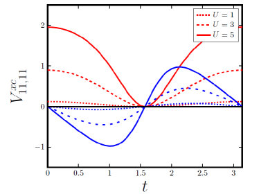
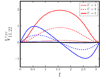
Figure 1: The real (red) and imaginary (blue) parts of the exchange-correlation potentials $V^{xc}_{11,11}$ and $V^{xc}_{11,22}$ of the Hubbard dimer as a function of time for $U=1,3,5$ with $\Delta=1$. Due to the particle-hole symmetry, $V_{xc}(-t)=-V_{xc}(t)$.

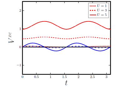
Figure 2: The real (red) and imaginary (blue) parts of the exchange-correlation potential in the bonding state $\phi_{B}=\frac{1}{\sqrt{2}}(\varphi_{1}+\varphi_{2})$ or anti-bonding state $\phi_{A}=\frac{1}{\sqrt{2}}(\varphi_{1}-\varphi_{2})$ as a function of time for $U=1,3,5$ with $\Delta=1$. Since only the components $V^{xc}_{11,11}=V^{xc}_{22,22}$ and $V^{xc}_{11,22}=V^{xc}_{22,11}$ exist, $V^{xc}_{BB,BB}=V^{xc}_{AA,AA}=\frac{1}{2}(V^{xc}_{11,11}+V^{xc}_{11,22})$. The imaginary part of $V_{xc}$ for $U=1$ is practically invisible.

Another interesting feature is the discontinuity of $V^{xc}$ at $t=0$, which is the difference between the particle ($t=0^{+}$) and the hole ($t=0^{-}$) values, reminiscent of the discontinuity in the exchange-correlation potential in density functional theory perdew1982 .

One also notices that the time dependence is dictated by the excitation energies of the $(N\pm 1)$ systems and in general, these excitations include collective ones. For example, for solids one expects a time-dependent term of the form $\exp(i\omega_{p}t)$ where $\omega_{p}$ is the plasmon energy. $V_{xc}$ acts then like an effective external field, exchanging an energy $\omega_{p}$ with the system, as illustrated more explicitly in the next example on the Holstein Hamiltonian.

III.2 Holstein Hamiltonian

A simplified Holstein Hamiltonian describing a coupling between a core electron and a set of Bosons, such as plasmons or phonons, is given by langreth1970

$$\hat{H}=\varepsilon\hat{c}^{\dagger}\hat{c}+\sum_{q}\hat{c}\hat{c}^{\dagger}g_{q}(\hat{b}_{q}+\hat{b}_{q}^{\dagger})+\sum_{q}\omega_{q}\hat{b}_{q}^{\dagger}\hat{b}_{q},$$ (51)

where $\varepsilon$ is the core electron energy, $\omega_{q}$ is the Boson energy of wave vector $q$, and $\hat{c}$ and $\hat{b}_{q}$ are respectively the core electron and the Boson operators. This Hamiltonian can be solved analytically and the algebra is simplified if it is assumed that the Boson is dispersionless with an average energy $\omega_{p}$. Under this assumption, the exact solution for the core-electron removal spectra yields langreth1970

$$A(\omega)=\sum_{n=0}^{\infty}f_{n}\delta(\omega-\varepsilon-\Delta\varepsilon+n\omega_{p}),$$ (52)

where

$$f_{n}=\frac{e^{-a}a^{n}}{n!},\;\;a=\sum_{q}\left(\frac{g_{q}}{\omega_{p}}\right)^{2},\;\;\Delta\varepsilon=a\omega_{p}.$$ (53)

This exact solution can also be obtained using the cumulant expansion bergersen1973 ; hedin1965 ; almbladh1983 . The hole Green function corresponding to the above spectra is given by

$$G(t<0)=i\sum_{n=0}^{\infty}f_{n}e^{-i(\varepsilon+\Delta\varepsilon-n\omega_{p})t}\theta(-t).$$ (54)

It can be verified that the time-dependent exchange-correlation potential corresponding to the Holstein Hamiltonian reads

$$V_{xc}(t<0)=\Delta\varepsilon\left(1-e^{i\omega_{p}t}\right).$$ (55)

This expression provides a very simple interpretation: the first term corrects the non-interacting core-electron energy whereas the second term describes the Bosonic mode interacting with the core electron, which can exchange not only one but multiple quanta of $\omega_{p}$ with the field. This is precisely what is accomplished by the cumulant expansion bergersen1973 ; hedin1965 ; almbladh1983 within the self-energy formulation but in an ad hoc manner.

IV Conclusion

The problem of calculating the self-energy is recast into the problem of constructing the exchange-correlation potential arising from the exchange-correlation hole, which is a physically motivated entity fulfilling an exact sum rule and some limiting properties. The proposed formalism is in the spirit of density functional theory, in which the main task is to find an accurate approximation for the exchange-correlation functional.

There are many aspects to explore and consider. For example, it would be interesting to investigate the degree of locality of $V_{xc}$, i.e., how $V_{xc}$ behaves as a function of $|\mathbf{r}^{\prime}-\mathbf{r}|$ and to study the time dependence of $V_{xc}$ for a number of model systems such as the electron gas and one-dimensional systems solvable by means of the Bethe ansatz in order to accumulate clues and guidelines for constructing an accurate and reliable $V_{xc}$ or $\rho_{xc}$.

- (1) See, for example, A. L Fetter and J. D Walecka, Quantum Theory of Many-Particle Systems, (Dover, Mineola, New York, 2003).
- (2) See, for example, J. W. Negele and H. Orland, Quantum Many-Particle Systems, (Westview Press, Boulder, Colorado, 1998).
- (3) P. Hohenberg and W. Kohn, Phys. Rev. 136, B864 (1964).
- (4) W. Kohn and L. J. Sham, Phys. Rev. 140, A1133 (1965).
- (5) R. O. Jones and O. Gunnarsson, Rev. Mod. Phys. 61, 689 (1989).
- (6) A. D. Becke, J. Chem. Phys. 140, 18A301 (2014).
- (7) J. C. Slater, Phys. Rev. 81, 385 (1951).
- (8) O. Gunnarsson and B. I. Lundqvist, Phys. Rev. B 13, (4274 1976).
- (9) J. C. Slater, Phys. Rev. 165, 658 (1968).
- (10) E. Runge and E. K. U. Gross, Phys. Rev. Lett. 52, 997 (1984).
- (11) For a review, see, for example, N. T. Maitra, J. Chem. Phys. 144, 220901 (2016).
- (12) J. A. Alonso and L. A. Girifalco, Phys. Rev. B 17, 3735 (1978).
- (13) O. Gunnarsson, M. Jonson, and B. I. Lundqvist, Phys. Rev. B 20, 3136 (1979).
- (14) L. J. Sham and W. Kohn, Phys. Rev. 145, 561 (1966).
- (15) D. C. Langreth and J. P. Perdew, Solid State Commun. 14, 1425 (1975).
- (16) See, for example, G. Stefanucci and R. van Leeuwen, Nonequilibrium Many-Body Theory of Quantum Systems: A Modern Introduction, (Cambridge University Press, 2013).
- (17) J. P. Perdew, R. G. Parr, M. Levy, and J. L. Balduz, Phys. Rev. Lett. 49, 1691 (1982).
- (18) D. C. Langreth, Phys. Rev. B 1, 471 (1970).
- (19) B. Bergersen, Can. J. Phys. 51, 102 (1973).
- (20) L. Hedin, Phys. Scr. 21, 477 (1980).
- (21) C.-O. Almbladh and L. Hedin, in Handbook on Synchroton Radiation, edited by E. E. Koch (North-Holland, Amsterdam, 1983) Vol. 1, p.686.