Evaluation of histological findings with severity grade, to analyze toxicology in-vivo studies

Abstract

In-vivo toxicological studies are characterized by multiple primary endpoints with quite different scales. Whereas guidelines and publications provide various statistical tests for normally distributed endpoints (such as organ weights) and proportions (such as tumor rates), few approaches are available for graded histopathological findings, such as 0, +, ++, +++. This represents a basic contradiction of the statistical analysis because these graded findings sometimes show a high predictive value for potential toxic effects. Here we discuss different methods comparatively, especially from the viewpoints of i) designs for very small sample sizes and ii) interpretability by toxicologists. A new approach is recommended where a simultaneous test is performed over all class combinations of score levels, such as (0, +) vs (++, +++). Corresponding R code is provided by way of a data example.

1 The problem

The basic dilemma in analyzing in-vivo toxicology studies is that both methods and software are available to analyze dose-response data of in-vivo assays, including the important zero-dose control, when data (to be precise: residuals) are normal-distributed, such as body or organ weights, but their toxicological relevance is often rather limited. More relevant toxicologically are proportions, such as mortality and tumor rates, or even more so, histological findings with severity grades. For the latter, rather few methods/software are available. As a rule of thumb, one can assume a sequence of statistical precision (e.g., in terms of power): normal $\rightarrow$ score $\rightarrow$. But frequently the reverse order is true for the toxicological relevance. This approach may be considered old-fashioned, however it is still practiced. Regardless, the three-cross system easily translates into numerical, ordered categorical values. In toxicology, the system is used to describe, for example, the severity of clinical or ophthalmological symptoms, where the crosses or numbers represent the adverbs ’minimal’, ’moderate’, and ’severe’. In such cases, no definition is attributed to these values yet it is important that these values be defined. In other cases, e.g., for hematology values, attempts have been made to define the grading by a range of deviations from a mean value established by control data [7]. Otherwise, there are guidances/guidelines describing the use of three-grade (plus 0) systems, e.g. to establish thyroid gland alterations in the amphibian metamorphosis assay [11], [1], [2]. In this specific case, each grade is defined by an alteration range, e.g., for thyroid atrophy: Grade 0 - less than a $20\%$ reduction in size in comparison to controls; Grade 1 - gland size is $30\%-50\%$ reduced from the size of control glands; Grade 2 - gland size is $60\%-80\%$ reduced from the size of control glands; Grade 3 - gland size is over $80\%$ reduced from the size of control glands. In addition, there are proposed systems based on zero and four severity degrees, where the values are quasi-defined, e.g., for the evaluation of local reactions due to the implantation of medical devices or their materials. In this case, examples are presented for the cell type and tissue reaction that are described, e.g., lymphocytes per high power field (hpf=magnification x400): grade 0: 0; grade 1: rare, 1-5 per hpf; grade 2: 5-10 per hpf; grade 3: marked infiltration; grade 4: packed.
Currently, a five-grade system (plus 0) is applied by almost all toxicological pathologists based on recommendations of Thoolen et al., 2010 [29]. The gradings should however be described, hence an STP best practice paper [24] on pathology report writing recommends: When severity grading is important to the understanding of major study findings, it may be useful to provide a description of the distinguishing features of each severity grade. In fact, an STP working group supports greater transparency and consistency in the reporting of grading scales and provided several recommendations on detailed severity criteria [27]. A published example by Weber et al. supports a graded scale, in this instance for pathological changes in the lungs [32].

Here we consider scores with only a few categories, e.g., $0,+,++,+++$. Again, the number of informative categories matters, i.e., a three-category score is more precise than a proportion (two categories) whereas $k>5$ category scores behave nearly like a normally distributed endpoint (whereby commonly not every individual category is informative in the respective assay). Several statistical approaches are available for scores or count data. The focus here is interpretability of both the effect size and its confidence interval [13].

1.1 A motivating example

As a simple motivating example, the liver basophilia severity scores data [10], Table 4 was selected.

Table 1: c-by-k Table Data of Liver Basophilia Severity Scores

	Severity	1	2	3
Dose
1		9	4	1
2		4	8	0
3		7	6	0
4		3	10	1
5		6	4	4

Dose=1 is the zero-dose control. Notice that no zero-severity score (0) is defined in this assay (somewhat curious in a toxicological bioassay or else the zero data have not been presented). Two questions should be answered in this context: i) is there a score change for any dose compared to the control and could this be in terms of a dose trend, and ii) is this score change with dose more likely from category 1 to 2, 2 to 3 or 1 to 3?

2 Discussion of several approaches to analyzing scores or count data

2.1 Classifications and assumptions

First, it may not seem too important but should we really use two-sided tests as proposed in some guidances and used commonly in publications? The answer is clearly no, both from a power argument (in designs with small $n_{i}$) and from the argument of problem-adapted interpretation (there is no interest in a possible dose-related shift from +++ to +). Appropriate and a-priori chosen one-sided tests should clearly be preferred in most scenarios in toxicological risk assessment.
A second question when evaluating the common design $[C;D_{1},...,D_{k}]$ is whether to use i) (one-sided) many-to-one comparisons of the Dunnett-type [8], ii) trend tests assuming the doses qualitatively in comparison to C-, i.e., Williams-type [33] or iii) trend tests assuming doses quantitatively, i.e., Tukey-type [26]. It may be an unconventional idea, but we recommend all three options simultaneously, i.e., answering an imprecisely formulated question for a possible dose-related toxicological effect by several models. One must pay a price in power loss for the multiplicity of such an approach. The power loss, however, is not too dramatic considering highly correlated tests and is outweighed by the advantage, broader interpretation possibility.
A third issue is how to transform the graded findings, $[0,+,++,+++]$, into ordered categorical data, $[0,1,2,3]$. It remains an ordinal response: 0 is less toxic than 1, etc. Several methods will be discussed. One selection aspect would by the min(p) idea, i.e., take the best. Toxicologists’ reasoning is more ’Is the trend caused by +++ shift alone, or jointly (++, +++), or…?’. Two serious constraints are common in such toxicological data: i) very small $n_{i}$, so small that asymptotic methods have problems (e.g., with FWER control), and ii) rather equal low score values in the control, i.e., $p_{0}=0$ is possible (and toxicologically not surprising), and thus data without variance, which causes massive convergence problems in the general linear model (GLM) logistic. A further limitation of the sliced Cochran-Armitage test is that it presents a test for an exactly linear trend, but in toxicology such a perfect linear dose-response relationship is quite rare in practice. Therefore, we propose several trend tests, both Tukey-type for dose as a quantitative covariate and Williams/Dunnett-type for dose as a qualitative factor for pooling patterns of the categories [14].

2.2 Using Dunnett, Williams or Tukey-type tests?

Confusingly, for the evaluation of the widely used design $[C-,D_{1},...,D_{k}]$ (where $D_{i}$ represents the administered doses and C- is the zero-dose control), some guidelines recommend the Dunnett’s test [8], others the Williams test [33], and occasionally, the Armitage test [4]. In the most commonly used Dunnett’s test, each dose is compared to C- (one-sided, e.g., for increase or in many cases, two-sided for any difference) with control of family-wise error rate for all these comparisons. In the Williams test, a monotone increase (or decrease) effect with increasing dose is tested in comparison to C- (usually one-sided), whereby an individual comparison to C- can only be interpreted for the maximum dose. The Armitage test is a trend test for a linear increase (or decrease) in proportions, such as tumor rates. As a special regression model, it takes the doses into account quantitatively, whereas Dunnett’s and Williams’ tests consider the doses as a qualitative factor. The disadvantage of the Armitage test, that it is only defined for linear alternatives and proportions, can be overcome with the Tukey test [30]. This simultaneously models linear, ordinal and logarithmic doses in the generalized linear model and is thus sensitive to a wide class of possible dose-response dependencies [26]. The choice of one of these tests is nontrivial and depends on the design, the question, and the data condition [14].

2.3 A nonparametric approach based on relative effect size

Nonparametric tests (e.g., Kruskal-Wallis or Mann-Whitney tests [34]) are commonly used for ordinal response data but tied data are considered only an approximation and confidence intervals are hard to obtain or to interpret. New proposals for related trend tests, e.g., Altunkaynak and Gamgam [3] suffer from the same issues. The relative effect size approach for multiple contrasts allows i) discrete data, ii) variance heterogeneity and iii) provides simultaneous confidence intervals [21]. A related CRAN library nparcomp is available [23]. Simple code for the example data, in this case for the Williams-type test [22], is:

library(nparcomp)
ko1<-nparcomp(Severity ~dose, data=green, asy.method = "mult.t",
            type = "Williams",alternative = "greater", info = FALSE)
summary(ko1)  # Reveal the adjusted p-values
plot(ko1)  # Plot simultaneous confidence limits

Adjusted p-values or simultaneous confidence intervals are available whereas the interpretation of relative effect size as success probability is challenging. The win odds ratio [5] may be an alternative for better understanding by toxicologists.

  Comparison Estimator Lower Upper Statistic    p.Value
1 p( 1 , 2 )     0.631 0.398     1 1.2770958 0.26414207
2 p( 1 , 3 )     0.536 0.309     1 0.3577455 0.65530831
3 p( 1 , 4 )     0.699 0.483     1 2.0936297 0.07009149
4 p( 1 , 5 )     0.638 0.416     1 1.4123519 0.21881077

2.4 Simple transformation model

Simple transformation of the endpoint allows the use of standard tests, such as Dunnett’s or Williams’. Here the Freeman-Tukey transformation [9] for count data is proposed for use in small sample designs in toxicology [12]. Such a simple approach is robust, particularly when using designs with small $n_{i}$, which represents a serious argument. Adjusted p-values or simultaneous confidence intervals are available but intervals are hard to interpret because back-transformation is not always obvious.

library("multcomp")
green$FT <-sqrt(green$Severity)+ sqrt(green$Severity+1)
modFT <-lm(FT~dose, data=green)
pvalFT <-summary(glht(modFT, linfct=mcp(dose="Dunnett"),alternative="greater"))

Adjusted p-values are available:

Linear Hypotheses:
           Estimate Std. Error t value Pr(>t)
2 - 1 <= 0  0.18475    0.17167   1.076 0.3468
3 - 1 <= 0  0.03458    0.16808   0.206 0.7312
4 - 1 <= 0  0.31374    0.16494   1.902 0.0943 .
5 - 1 <= 0  0.28239    0.16494   1.712 0.1341

2.5 Generalized linear model

The generalized linear model (GLM) is the first line natural approach for such count data, particularly using the flexible quasi-Poisson link function. However, this model is only defined asymptotically. With the object-oriented properties within R, the estimation of a GLM object can be easily imported into the function glht() in the multcomp package, based on the theory of simultaneous inference in general parametric models [18].

library("multcomp")
exP <-glm(Severity~dose, data=green, family=quasipoisson(link = "log"))
pvalGLM <-summary(glht(exP, linfct=mcp(dose="Dunnett"), alternative="greater"))

Adjusted p-values or simultaneous confidence intervals are available, where the effect size is the odds ratio.

Linear Hypotheses:
           Estimate Std. Error z value Pr(>z)
2 - 1 <= 0  0.15415    0.15472   0.996  0.367
3 - 1 <= 0  0.02281    0.15674   0.146  0.739
4 - 1 <= 0  0.26236    0.14552   1.803  0.105
5 - 1 <= 0  0.26236    0.14552   1.803  0.105

2.6 Cumulative link model

The cumulative link model is based on the assumption that an ordinal endpoint $Z_{ij}$ falls into $j=1,\ldots,J$ categories in each of $i$ groups and follows a multinomial distribution with the parameters $\pi_{ij}$. Then the cumulative probabilities $Pr(Z_{i}\leq j)=\pi_{i1}+\ldots+\pi_{ij}$ can be defined accordingly with cumulative logits: $\textup{logit}(Pr(Z_{i}\leq j))=\log\frac{Pr(Z_{i}\leq j)}{1-Pr(Z_{i}\leq j)}$. This framework can be used within regression models independently for each $j$ with the package |ordinal| [6]. Particularly, using the |clm| function the parameter of a cumulative link model can be fitted whereas the endpoint severe is defined as an ordered categorical. The effect sizes are cumulative log-odds ratios and the parameter estimates are differences from control (abbreviated with $1$)). Therefore, Wald-type confidence intervals can be estimated in case Bonferroni adjustments for a Dunnett-type approach were used level $(1-0.05/2)$ because of four one-sided rather than two-sided comparisons.

GreenCLM <- clm(sever ~ dose, data=green)
propCI <-exp(confint(GreenCLM, level=1-0.05/2)) # Bonferroni odds ratio CI

All simultaneous lower limits are less than one, i.e., no increasing severity from category $1\Rightarrow 2$ and $2\Rightarrow 3$ occur in the comparison of any dose with respect to control.

2.7 Ordered categorical regression

The ordered categorical regression model estimates the proportional log-odds ratio for both the treatment contrast estimates and the intercepts [17]. Using the Polr function that comes with the CRAN package tram, these estimates are available and can be used easily by the object properties for simultaneous inference, doses vs. control, in the function glht:

library(multcomp)
library(tram)
green$score<-as.ordered(green$Severity)
PL2<-polr(score ~ dose, data =green)
summary(PL2)
summary(glht(PL2, linfct=mcp(dose="Dunnett"),
                     alternative="greater"))

Adjusted p-values or simultaneous confidence intervals are available, where the effect size is the odds ratio.

Linear Hypotheses:
           Estimate Std. Error z value Pr(>z)
2 - 1 <= 0   0.9630     0.7743   1.244 0.2686
3 - 1 <= 0   0.2863     0.7743   0.370 0.6510
4 - 1 <= 0   1.4950     0.7628   1.960 0.0767 .
5 - 1 <= 0   1.3631     0.8102   1.682 0.1324

2.8 Multinomial model

A further modeling option is to define the scores as a multinomial vector [25]. The VGAM package allows fitting multinomial models by the vglm() function, whereas several R-functions provide simultaneous inference between both treatment contrasts and categories [31]:

library(VGAM)
green$C1 <- ifelse(green$Severity == 1, 1, 0)
green$C2 <- ifelse(green$Severity == 2, 1, 0)
green$C3 <- ifelse(green$Severity == 3, 1, 0)
multivgam <- vglm(cbind(C1,C2,C3) ~ dose,
family=multinomial(refLevel=1), data=green)
summary(glht(model = multin2mcp(multivgam, dispersion="overall"),
linfct = mcp2matrix(multivgam, linfct = mcp(dose = "Dunnett"))$K, alternative="greater"))
@

The estimated adjusted p-values reveal a non-significant effect for comparing dose 4 vs. control for the comparison of categories $C2/C1$. Notice the extreme variance estimators due to too low variance in doses 1 and 2 for $C3/C1$.

Linear Hypotheses:
                   Estimate Std. Error t value Pr(>t)
C2/C1: 2 - 1 <= 0    1.5041     0.8044   1.870 0.1961
C2/C1: 3 - 1 <= 0    0.6568     0.7678   0.855 0.7302
C2/C1: 4 - 1 <= 0    2.0149     0.8357   2.411 0.0604 .
C2/C1: 5 - 1 <= 0    0.4055     0.8269   0.490 0.8840
C3/C1: 2 - 1 <= 0  -15.1809  1688.2201  -0.009 0.9788
C3/C1: 3 - 1 <= 0  -15.5521  1536.4467  -0.010 0.9788
C3/C1: 4 - 1 <= 0    1.0986     1.4659   0.749 0.7822
C3/C1: 5 - 1 <= 0    1.7918     1.1589   1.546 0.3405

2.9 Most likely transformation model, special for count data

To overcome 1st moment modeling, adjusting or ignoring the other moments of the distribution allows the most likely transformation (MLT) model [17]. Count data are particularly sensitive to the underlying assumption, e.g., for ties and variance heterogeneity structure, and therefore a special MLT approach for counts was recently proposed [28]. The CRAN package cotram offers flexible count transformation models where count responses may arise from various and complex data-generating processes. Again, using R’s object-oriented properties, the estimate of a cotram object can be easily imported into the function glht() in the multcomp package.

library(cotram)
NSH<-cotram(Severity~dose, data=green,order=2)
WISH<-glht(NSH, linfct = mcp(dose = "Dunnett"), alternative="greater")

Adjusted p-values or simultaneous confidence intervals are available, where the effect size is the odds ratio.

Linear Hypotheses:
           Estimate Std. Error z value Pr(>z)
2 - 1 <= 0   0.9815     0.7790   1.260 0.2635
3 - 1 <= 0   0.2901     0.7765   0.374 0.6508
4 - 1 <= 0   1.5316     0.7700   1.989 0.0723 .
5 - 1 <= 0   1.3796     0.8150   1.693 0.1304

3 A new proposal: multiple contrast test based on multiple correlated binary data

This new proposal based on five items. First, collapsing of certain categories to obtain a toxicologists-like interpretability [10]. Secondly, rather than using independent Cochran-Armitage tests for the resulting proportions as in [10] (cherry-picking style for the p-values), these cut-point-selected categories are considered multiple correlated proportions and are analyzed jointly [13]. A third item is the use of multiple unrestricted Dunnett-type [8] or order-restricted Williams-type [33] contrast tests [13] but not trend tests solely for a linear dose-response relationship (note that the title of Armitage’s paper is Tests for linear trends in proportions). Fourthly, use permutation tests within the framework of conditional inference [19] to achieve an appropriate test for small $n_{i}$ without possible variance in the control (and/ or lower dose) groups for multiple correlated endpoints- a permutative max(max-test)) [15]. Finally, R-code should be available, using elementary R-code for categorization and the library(coin) [20] for simultaneous inference.
To demonstrate this new approach, a more realistic data example was used, namely the scores of Gon Phenotype in the dataset exampleHistData within the library(RSCABS) for F1 males in week 8 for the full-sample size treatment groups 1 (control), 2,4,5.

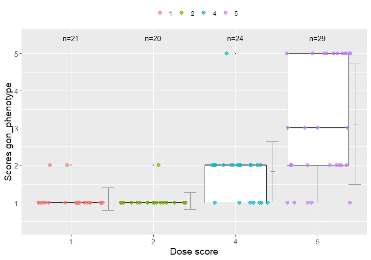
Figure 1: Boxplot with scores values

The related R-code for a one-sided Dunnett-type test is for the three categories EP1, EP2, EP3, jointly:

library(RSCABS)
data(exampleHistData)
subIndex<-which(exampleHistData$Generation==’F1’ &
exampleHistData$Genotypic_Sex==’Male’ &
exampleHistData$Age==’8_wk’)
LH<-exampleHistData[subIndex, ]
lh<-LH[, c(2,6)]
lh$Gon<-as.numeric(lh$Gon_Phenotype)
lh$EP1<-ifelse(lh$Gon >1,1,0)
lh$EP2<-ifelse(lh$Gon >2,1,0)
lh$EP3<-ifelse(lh$Gon >3,1,0)
lh$treat<-as.factor(lh$Treatment)
lhh<-droplevels(lh[lh$treat!=6, ])
Lhh<-droplevels(lhh[lhh$treat!=3, ])

library("coin")
library("multcomp")
Co1 <- function(data) trafo(data, factor_trafo = function(x)
 model.matrix(~x - 1) %*% t(contrMat(table(x), "Dunnett")))
Codu <-independence_test(EP1 +EP2+EP3~ treat, data = Lhh, teststat = "maximum",
distribution = "approximate", xtrafo=Co1, alternative="greater")
pvalCODU <-pvalue(Codu, method="single-step")
pvalCODU

The actual test is brief in the last eight lines: i+ii) packet calls, iii+iv) Dunnett-type contrast matrix, v+vi) multiple endpoint resampling max(max-test)), vii, viii) adjusted p-values for contrast and categories, namely:

          Gon     EP1     EP2     EP3
2 - 1  0.9284  0.9463  0.9137  0.9216
4 - 1  0.2269  0.0001  0.8750  0.8570
5 - 1 <0.0001 <0.0001 <0.0001 <0.0001

The interpretation of these adjusted p-values is intuitive: i) in principle the comparison of the high dose 5 vs. control always shows an increasing, strongly significant effect (globally seen independently of the cut-off), ii) on the other hand the low dose (2) shows no effect at all (no matter which cut-off was considered), and iii) an increase is shown exactly only for cut-off 1 vs. (2, 3, 5); for the medium dose 4, small changes in severity $>1$ already cause a significant effect - a toxicologically relevant finding.
This approach can be slightly modified for a Williams-type trend test and for simultaneous consideration of the score data itself in a Wilcoxon-type permutation test.

CoW <- function(data) trafo(data, factor_trafo = function(x)
 model.matrix(~x - 1) %*% t(contrMat(table(x), "Williams")))
Cowi <-independence_test(EP1 +EP2+EP3~ treat, data = Lhh, teststat = "maximum",
distribution = "approximate", xtrafo=CoW, alternative="greater")
pvalCOWI <-pvalue(Cowi, method="single-step")
pvalCOWI

      EP1     EP2     EP3
C 1 <1e-04 <0.0001 <0.0001
C 2 <1e-04  0.0004  0.0036
C 3 <1e-04  0.0089  0.0386

Monotone increasing trends exist for any category, whereas the strongest for 1, (2,3,5).

Adu <-independence_test(Gon+EP1 +EP2+EP3~ treat, data = Lhh, teststat = "maximum",
distribution = "approximate", xtrafo=Co1, alternative="greater")
pvalADU <-pvalue(Adu, method="single-step")
pvalADU

          Gon     EP1     EP2     EP3
2 - 1  0.9331  0.9517  0.9191  0.9264
4 - 1  0.2274 <0.0001  0.8821  0.8658
5 - 1 <0.0001 <0.0001 <0.0001 <0.0001

A significant difference of the highest dose vs. control is also shown for the score data per se. For the first data example the R-code is:

library("coin")
library("multcomp")
green$treat<-as.factor(green$Dose)
Co1 <- function(data) trafo(data, factor_trafo = function(x)
 model.matrix(~x - 1) %*% t(contrMat(table(x), "Dunnett")))
gCodu <-independence_test(S12 +S23~ treat, data = green, teststat = "maximum",
distribution = "approximate", xtrafo=Co1, alternative="greater")
pvalGCODU <-pvalue(gCodu, method="single-step")

The adjusted p-values for the proportions S12 and S23 are:

        S12    S23
2 - 1 0.9891 0.2772
3 - 1 0.9899 0.8290
4 - 1 0.9643 0.0707
5 - 1 0.2122 0.5731

3.1 Modified approach considering dose as a quantitative covariate

Dose can be considered as qualitative factor using multiple contrast tests or as a quantitative covariate using linear or nonlinear dose-response models. A specific one-parametric slope fitting model approach, which allows a simplified interpretation and yet covers a wide range of dose-response models is Tukey’s [30], i.e., the maximum of untransformed, log-transformed, or ordinal-transformed dose scores [26]. This can also applied for multiple correlated proportions as asymptotic GLM-based models (but is only asymptotically valid) [16]. Again, the R code is intuitive and relatively simple, assuming dose values of 0,10,50, and 150 in the above example:

library(tukeytrend)
library(multcomp)

Lhh$Dose<-as.numeric(as.character(Lhh$Treatment))
Lhh$dose[Lhh$Dose==1] <-0
Lhh$dose[Lhh$Dose==2] <-10
Lhh$dose[Lhh$Dose==4] <-50
Lhh$dose[Lhh$Dose==5] <-150

bx1<-glm(EP1~dose, data=Lhh, family=binomial(logit))
bx2<-glm(EP2~dose, data=Lhh, family=binomial(logit))
bx3<-glm(EP3~dose, data=Lhh, family=binomial(logit))
tx1 <- tukeytrendfit(bx1, dose="dose", scaling=c("ari", "ord", "arilog"))
tx2 <- tukeytrendfit(bx2, dose="dose", scaling=c("ari", "ord", "arilog"))
tx3 <- tukeytrendfit(bx3, dose="dose", scaling=c("ari", "ord", "arilog"))
tx <- combtt(tx1, tx2, tx3)
TX <- summary(asglht(tx))
@

A specific fitting one-parametric slope interpretation is already more complex: multiple models and multiple cut-points:

Linear Hypotheses:
                                        Estimate Std. Error t value Pr(>|t|)
tx1.glm.EP1.doseari: doseari == 0       0.025103   0.005065   4.956  < 0.001 ***
tx1.glm.EP1.doseord: doseord == 0       1.618118   0.312682   5.175  < 0.001 ***
tx1.glm.EP1.dosearilog: dosearilog == 0 1.444525   0.261639   5.521  < 0.001 ***
tx2.glm.EP2.doseari: doseari == 0       0.036360   0.009961   3.650  0.00143 **
tx2.glm.EP2.doseord: doseord == 0       3.278679   1.043687   3.141  0.00737 **
tx2.glm.EP2.dosearilog: dosearilog == 0 2.942857   0.966542   3.045  0.00936 **
tx3.glm.EP3.doseari: doseari == 0       0.031547   0.009878   3.194  0.00610 **
tx3.glm.EP3.doseord: doseord == 0       2.768226   1.019649   2.715  0.02431 *
tx3.glm.EP3.dosearilog: dosearilog == 0 2.464308   0.943507   2.612  0.03207 *

The most sensitive is for the cut-point 1 vs 2,3,5 for the logarithmic dose score.

4 Summary

A new permutation test for analyzing histopathologic findings with severity based on their decomposition into multiple correlated proportions for multiple Dunnett or Williams-type contrasts is presented. The focus is on problem-adequate interpretation and use for small $n_{i}$ designs with possibly reduced variance in the control. An asymptotic variant for simple quasilinear models is also available, allowing a wide class of possible dose-response dependencies to be evaluated. Due to the use of the CRAN packages coin, tukeytrend and multcomp, the evaluation of real data is relatively easy.
The next future work is simulation for small $n_{i}$ designs with different data conditions up to zero-variance in the control.

References

- [1] Organisation for Economic Co-operation and Development (OECD). Histopathology Guidance Document for the Larval Amphibian Growth and Development Assay (LAGDA). Draft, Dec. 2014. http://www.oecd.org/env/ehs/testing/Histopatholoy-Guidance-Document-for-the-Larval-Amphibian-Growth-and-Development-Assay.pdf. Accessed: 01-April-2019., 2014.
- [2] http://www.oecd.org/env/ehs/testing/Histopatholoy-Guidance-Document-for-the-Larval-Amphibian-Growth-and-Development-Assay.pdf. Accessed: 01-April-2019., 2019.
- [3] Bulent Altunkaynak and Hamza Gamgam. npordtests: An R Package of Nonparametric Tests for Equality of Location Against Ordered Alternatives. R JOURNAL, 12(1):147–171, JUN 2020.
- [4] P. Armitage. Tests for linear trends in proportions and frequencies. Biometrics, 11(3):375–386, 1955.
- [5] E. Brunner, M. Vandemeulebroecke, and T. Mutze. Win odds: An adaptation of the win ratio to include ties. Statistics in Medicine, 40(14):3367–3384, June 2021.
- [6] R.H.B. Christensen. Cumulative link models for ordinal regressionwith the r package ordinal. J. Stat. Software (submitted), 2020.
- [7] M. de Kort, K. Weber, B. Wimmer, K. Wilutzky, P. Neuenhahn, and P.n Metamorphosis Allingham. Historical control data for hematology parameters obtained from toxicity studies performed on different wistar rat strains: Acceptable value ranges, definition of severity degrees, and vehicle effects. Toxicol Res Appl. 2020;4: 1–32., 2020.
- [8] C. W. Dunnett. A multiple comparison procedure for comparing several treatments with a control. J Am Stat Assoc, 50(272):1096–1121, 1955.
- [9] MF Freeman and JW Tukey. Transformations related to the angular and squre root. Ann. Meth. Stat., 21(2):305, 1950.
- [10] J. W. Green, T. A. Springer, A. N. Saulnier, and J. Swintek. Statistical analysis of histopathological endpoints. Environmental Toxicology and Chemistry, 33(5):1108–1116, May 2014.
- [11] K.C. Grim, M. Wolfe, T. Braunbeck, T. Iguchi, Y. Ohta, O. Tooi, and L. Touart. Thyroid histopathology assessments for the amphibian metamorphosis assay to detect thyroid-active substances. Toxicol Pathol. 2009;37(4): 415-424., 2009.
- [12] L. A. Hothorn, K. Reisinger, T. Wolf, A. Poth, D. Fieblingere, M. Liebsch, and R. Pirow. Statistical analysis of the hen’s egg test for micronucleus induction (het-mn assay). Mutation Research-Genetic Toxicology and Environmental Mutagenesis, 757(1):68–78, September 2013.
- [13] L.A. Hothorn. Statistics in Toxicology- using R. CRC Press, 2016.
- [14] L.A. Hothorn. Claiming trend in toxicological and pharmacological dose-response studies: an overview on statistical methods and related r-software. ArXiv:2007.09631 (2020), 2020.
- [15] L.A. Hothorn and S. Kropf. Closed testing procedures for treatment-versus-control comparisons and multiple correlated endpoints. arXiv:submit/3648293, 2021.
- [16] L.A. Hothorn, C. Ritz, and F. Schaarschmidt. A vignette for cran package tukeytrend in general paramertic models. Report Leibniz University Hannover, 2018.
- [17] T. Hothorn. Most likely transformations: The mlt package. Journal of Statistical Software, 92(1):1–68, February 2020.
- [18] T. Hothorn, F. Bretz, and P. Westfall. Simultaneous inference in general parametric models. Technical report, 2008.
- [19] T. Hothorn, K. Hornik, M. A. Van de Wiel, and A. Zeileis. A lego system for conditional inference. American Statistician, 60(3):257–263, August 2006.
- [20] T. Hothorn, K. Hornik, M:A: van de Wiel, and A. Zeileis. Implementing a class of permutation tests: The coin package. Journal of Statistical Software, 28(8):1–23, 2008.
- [21] F. Konietschke and L. A. Hothorn. Rank-based multiple test procedures and simultaneous confidence intervals. Electronic Journal of Statistics, 6:738–759, 2012.
- [22] F. Konietschke and L.A. Hothorn. Evaluation of toxicological studies using a non-parametric Shirley-type trend test for comparing several dose levels with a control group. Stat Biopharm Res, 4:14–27, 2012.
- [23] F. Konietschke, M. Placzek, F. Schaarschmidt, and L. A. Hothorn. nparcomp: An r software package for nonparametric multiple comparisons and simultaneous confidence intervals. Journal of Statistical Software, 64(9), March 2015.
- [24] Daniel Morton, Ramon K Kemp, Sabine Francke-Carroll, Karl Jensen, Jeffrey McCartney, Thomas M Monticello, Richard Perry, Olga Pulido, Nigel Roome, Ken Schafer, et al. Best practices for reporting pathology interpretations within glp toxicology studies. Toxicologic pathology, 34(6):806–809, 2006.
- [25] F. Schaarschmidt, D. Gerhard, and C. Vogel. Simultaneous confidence intervals for comparisons of several multinomial samples. Computational Statistics and Data Analysis, 106:65–76, February 2017.
- [26] F. Schaarschmidt, C. Ritz, and L.A. Hothorn. The tukey trend test: Multiplicity adjustment using multiple marginal models. Biometrics, 2021.
- [27] Kenneth A Schafer, John Eighmy, James D Fikes, Wendy G Halpern, Renee R Hukkanen, Gerald G Long, Emily K Meseck, Daniel J Patrick, Michael S Thibodeau, Charles E Wood, et al. Use of severity grades to characterize histopathologic changes. Toxicologic pathology, 46(3):256–265, 2018.
- [28] S. Siegfried and T. Hothorn. Count transformation models. Methods in Ecology and Evolution, 11(7):818–827, July 2020.
- [29] Bob Thoolen, Robert R Maronpot, Takanori Harada, Abraham Nyska, Colin Rousseaux, Thomas Nolte, David E Malarkey, Wolfgang Kaufmann, Karin Küttler, Ulrich Deschl, et al. Proliferative and nonproliferative lesions of the rat and mouse hepatobiliary system. Toxicologic pathology, 38(7_suppl):5S–81S, 2010.
- [30] J. W. Tukey, J. L. Ciminera, and J. F. Heyse. Testing the statistical certainty of a response to increasing doses of a drug. Biometrics, 41(1):295–301, 1985.
- [31] C. Vogel. Simultaneous inference for the comparison of overdispersed multinomial data. Ph.D thesis Leibniz University, 2018.
- [32] Klaus Weber, Axel Bosch, Mario Bühler, Chirukandath Gopinath, Jerry F Hardisty, Nils Krueger, Ernest E McConnell, and Günter Oberdörster. Aerosols of synthetic amorphous silica do not induce fibrosis in lungs after inhalation: Pathology working group review of histopathological specimens from a subchronic 13-week inhalation toxicity study in rats. Toxicology Research and Application, 2:2397847318805273, 2018.
- [33] D. A. Williams. Test for differences between treatment means when several dose levels are compared with a zero dose control. Biometrics, 27(1):103–, 1971.
- [34] Takafumi Yamaguchi, Minoru Maeda, Keiko Ogata, Jun Abe, Toru Utsumi, and Koji Kimura. The effects on the endocrine system under hepatotoxicity induction by phenobarbital and di(2-ethylhexyl)phthalate in intact juvenile male rats. J. Tox. Sci, 44(7-9):459–469, 2019.