Optimized Two-Baryon Operators in Lattice QCD

Abstract

A set of optimized interpolating operators which are dominantly coupled to each eigenstate of two baryons on the lattice is constructed by the HAL QCD method. To test its validity, we consider heavy dibaryons $\Omega_{3Q}\Omega_{3Q}$ ($Q=s,c$) calculated by (2+1)-flavor lattice QCD simulations with nearly physical pion mass. The optimized two-baryon operators are shown to provide effective energies of the ground and excited states separately stable as a function of the Euclidean time. Also they agree to the eigenenergies in a finite lattice box obtained from the leading-order HAL QCD potential $V({\bm{r}})$ within statistical errors. The overlapping factors between the optimized sink operators and the state created by the wall-type source operator indicate that $V({\bm{r}})$ can be reliably extracted, no matter whether the spacetime correlation of two baryons is dominated by the ground state or the excited state. It is suggested that the optimized set of operators is useful for variational studies of hadron-hadron interactions.

I Introduction

Accurate determination of hadron-hadron interactions from QCD is one of the most challenging problems in nuclear and particle physics Drischler et al. (2021); Aoki and Doi (2020). To achieve the goal, two theoretical methods have been proposed in lattice QCD (LQCD); the Lüscher’s finite volume method Luscher (1991) and the HAL QCD method Ishii et al. (2007); Aoki et al. (2010); Ishii et al. (2012). The former focuses on the temporal behavior of the hadronic correlations, from which the scattering phase shifts are extracted through the Lüscher’s finite volume formula. On the other hand, the latter considers the spacetime behavior of the hadronic correlations, from which physical observables are extracted through the equal-time Nambu-Bethe-Salpeter (NBS) amplitude, or the NBS wave function in short.

Although these two methods are like looking at the two sides of the same coin and are theoretically related with each other, it has been realized that the “naive” plateau fitting in the Lüscher’s finite volume method without variational analysis sometimes leads to misleading results for two-baryon systems. It originates from the fact that separating the ground state from excited states of two baryons below inelastic threshold is exponentially difficult on the lattice as the splitting in energy becomes zero in the large volume limit Lepage (1990): Detailed account of this issue is given in Refs. Iritani et al. (2016, 2019a) (see also, Refs. Francis et al. (2019); Hörz et al. (2021); Amarasinghe et al. (2021)).

In contrast, the time-dependent version of the HAL QCD method Ishii et al. (2012) does not need to identify each level, since the same NBS integral kernel (i.e. the energy-independent non-local potential) governs all the elastic scattering states simultaneously. In other words, any superposition of the NBS wave functions of different energies below inelastic threshold leads to the same non-local potential. By using this nice property, one can construct a set of optimized interpolating operators and make a firm connection between the Lüscher’s finite volume method and the HAL QCD method for two baryons, as demonstrated in the (2+1)-flavor LQCD simulations with heavy pion mass, $m_{\pi}\simeq$ 510 MeV, and the lattice volumes, (3.6, 4.3, 5.8 fm)³ Iritani et al. (2019a). Such optimized operators can also be used to check the validity of the derivative expansion of the non-local potential in the HAL QCD method.

The purpose of this paper is to further explore the idea of optimized operators proposed in Ref. Iritani et al. (2019a) and study whether it is applicable to (2+1)-flavor LQCD near the physical pion mass, $m_{\pi}\simeq$ 146 MeV, with a large lattice volume, (8.1 fm)³. We consider two heavy dibaryons $\Omega_{3Q}\Omega_{3Q}$ in the ${}^{1}S_{0}$ channel with $Q=s$ and $c$, where $\Omega_{3Q}$ implies the spin-3/2 baryon composed of three valence quarks with flavor $Q$. Both systems are in the unitary regime with large scattering lengths as demonstrated recently by the $(2+1)$-flavor LQCD simulations Gongyo et al. (2018); Lyu et al. (2021). The statistical errors in these systems are relatively small in comparison to the baryons with light valence quarks, so that one can make quantitative analysis on the effect of the optimized operators as well as on the uncertainty due to derivative expansion of the non-local potential.

This paper is organized as follows. After a brief review of the HAL QCD method in Sec. II, we introduce a general framework to define the optimized two-baryon operators through the HAL QCD potential in Sec. III. Details of our lattice setup are given in Sec. IV. Numerical results and discussions on eigenfunctions, effective energies and the overlapping factors for $\Omega_{3Q}\Omega_{3Q}$ are presented in Sec. V. Sec. VI is devoted to summary and concluding remarks. The analyses for the higher excited states are given in Appendix. A.

II The HAL QCD Method

The equal time NBS amplitude for two Omega baryons with energy $E$ is defined in the Euclidean spacetime as

$$\Psi_{E}(\bm{r})e^{-Et}=\frac{1}{Z_{\Omega}}\sum_{\bm{x}}\braket{0}{\hat{\Omega}(\bm{x}+\bm{r},t)\hat{\Omega}(\bm{x},t)}{2\Omega,E},$$ (1)

where $\hat{\Omega}$ is a local interpolating operator for $\Omega\equiv\Omega_{3Q}$ ($Q=s$ and $c$) whose explicit form can be found in Refs. Gongyo et al. (2018); Lyu et al. (2021). $Z_{\Omega}$ is the wave function renormalization factor and $\ket{2\Omega,E}$ is the $2\Omega$ eigenstate with the center of mass energy $E=2\sqrt{m_{\Omega}^{2}+k^{2}}$.

Using Eq.(1) and the Haag-Nishijima-Zimmermann reduction formula for composite particles Zimmermann (1987), the interaction between baryons can be identified as the energy-independent non-local potential $U(\bm{r},\bm{r}^{\prime})$ in the equal-time NBS equation  Ishii et al. (2007); Aoki et al. (2010):

$$\frac{1}{m_{\Omega}}(k^{2}+\nabla^{2})\Psi_{E}(\bm{r})=\int d\bm{r}^{\prime}U(\bm{r},\bm{r}^{\prime})\Psi_{E}(\bm{r}^{\prime}).$$ (2)

In the time-dependent HAL QCD method Ishii et al. (2012); Aoki et al. (2013), the spacetime correlation function $R(\bm{r},t)$ is introduced as a linear superposition of the NBS wave functions below the inelastic threshold;

$$\begin{split}R(\bm{r},t)&={\sum_{\bm{x}}\braket{0}{\hat{\Omega}(\bm{x}+\bm{r},t)\hat{\Omega}(\bm{x},t)\overline{\mathcal{J}}(0)}{0}}/{(Z_{\Omega}e^{-2m_{\Omega}t})}\\ &=\sum_{n}a_{n}\Psi_{E_{n}}(\bm{r})e^{-(\Delta E_{n})t}+O(e^{-(\Delta E^{*})t}).\end{split}$$ (3)

Here $E_{n}$ is the eigenenergy of the $n$-th elastic scattering state in a finite box, and $\Delta E_{n}=E_{n}-2m_{\Omega}$ with $\Delta E_{n}\leq\Delta E^{*}$: The inelastic threshold is denoted by $\Delta E^{*}\sim\Lambda_{\mathrm{QCD}}\sim 300~{}\mathrm{MeV}$. The overlapping factors $a_{n}=\braket{2\Omega,E_{n}}{\overline{\mathcal{J}}(0)}{0}$ depend on the choice of the source operator $\overline{\mathcal{J}}(0)$ at $t=0$. If $t\gg(\Delta E^{*})^{-1}\sim 0.7$ fm, effects from the inelastic states are exponentially suppressed as $O(e^{-(\Delta E^{*})t})$, so that one can rewrite Eq.(2) into the time-dependent HAL QCD equation,

$$\left(\frac{1}{4m_{\Omega}}\frac{\partial^{2}}{\partial t^{2}}-\frac{\partial}{\partial t}-H_{0}\right)R(\bm{r},t)=\int d\bm{r}^{\prime}U(\bm{r},\bm{r}^{\prime})R(\bm{r}^{\prime},t),$$ (4)

with $H_{0}=-\nabla^{2}/m_{\Omega}$. The advantage of this equation is that we do not need to separate each eigenenergy $E_{n}$ to extract the potential $U$. Since the potential is spatially localized in QCD by construction, its finite volume correction is exponentially suppressed for large lattice volume. It has been also demonstrated in Refs. Iritani et al. (2019a, b) that observables (such as the phase shifts) do not depend on the choice of source operators $\overline{\mathcal{J}}(0)$ (either wall-type source or smeared source) by taking the $\Xi\Xi$ system as an example with the lattice volumes $\simeq(3.6,4.3,5.8\ {\rm fm})^{3}$ and $m_{\pi}\simeq$ 510 MeV, as long as the non-locality of the potential is well approximated by the derivative expansion.

We note that it is practically useful to make a derivative expansion of the non-local potential as

$$U(\bm{r},\bm{r}^{\prime})=V({\bm{r}})\delta(\bm{r}-\bm{r}^{\prime})+\sum_{n=1}V_{2n}(\bm{r})\nabla^{2n}\delta(\bm{r}-\bm{r}^{\prime}).$$ (5)

Then the leading-order (LO) potential is obtained as

$$V({\bm{r}})=R^{-1}(\bm{r},t)\left(\frac{1}{4m_{\Omega}}\frac{\partial^{2}}{\partial t^{2}}-\frac{\partial}{\partial t}-H_{0}\right)R(\bm{r},t).$$ (6)

III Optimized Sink Operators

Once the HAL QCD potential is obtained from the LQCD simulation of $R({\bm{r}},t)$ in Eq.(4), one can calculate eigenfunctions and eigenenergies in a finite lattice box by solving Eq.(2). This enables us to construct a set of optimized interpolating operators which couple strongly to each eigenstate, as originally proposed in Ref. Iritani et al. (2019a). We now apply this idea to find optimized sink operators in the present systems.

Let us first rewrite Eq.(2) in a three-dimensional lattice box by introducing the Hamiltonian $H$ with the discretized Laplacian $H_{0}$ and the non-local potential $U(\bm{r},\bm{r}^{\prime})$;

$$H=H_{0}+U,\quad H\Psi_{E_{n}}=\varepsilon_{n}\Psi_{E_{n}},$$ (7)

where $\varepsilon_{n}$ is related to $\Delta E_{n}$ as

$$\Delta E_{n}=2(\sqrt{\varepsilon_{n}m_{\Omega}+m_{\Omega}^{2}}-m_{\Omega}).$$ (8)

From the $n$-th NBS wave function $\Psi_{E_{n}}(\bm{r})$ for Hermitian matrix $U(\bm{r},\bm{r}^{\prime})$, one may construct an optimized sink operator as a projection to each $n$-th state,

$$S_{n}(t)=\sum_{\bm{r}}\Psi_{E_{n}}^{\dagger}(\bm{r})\left[\sum_{\bm{x}}\hat{\Omega}(\bm{x}+\bm{r},t)\hat{\Omega}(\bm{x},t)\right].$$ (9)

This is expected to couple primarily to $\ket{2\Omega,E_{n}}$ for large $t$. Two-baryon temporal correlation after the projection reads

$$R_{n}(t) = \sum_{\bm{r}}\Psi_{E_{n}}^{\dagger}(\bm{r})R(\bm{r},t),$$ (10)

$$= a_{n}e^{-(\Delta E_{n})t}+O(e^{-(\Delta E^{*})t}),$$

which can be used to extract effective two-baryon energy for each $n$ as

$$\Delta E^{\mathrm{eff}}_{n}(t)=\frac{1}{a}\ln\left[\frac{R_{n}(t)}{R_{n}(t+1)}\right].$$ (11)

This quantity should have plateau structure as a function of $t$ and approach to $\Delta E_{n}$ in Eq.(8) for large $t$. Note that the projection to each eigenstate is possible only if we have spatial information of the correlation function $R({\bm{r}},t)$. For similar attempts based on the spatial information of the correlation function in different physical contexts, see Refs. Umeda et al. (2001); Larsen et al. (2020); Chen et al. (2021).

In the case where only the LO potential $V(\bm{r})$ in Eq.(6) is available, eigenfunction $\psi_{n}(\bm{r})$ from the LO Hamiltonian $H_{\rm LO}\equiv H_{0}+V$ is an approximation of the exact $n$-th NBS wave function $\Psi_{E_{n}}(\bm{r})$. Hence resultant quantities in Eqs.(8)-(11) are approximate ones. Then, whether $\Delta E^{\mathrm{eff}}_{n}(t)$ has a plateau and approaches to Eq.(8) at large $t$ provide a confidence test on the truncation of the derivative expansion of $U$.

For later purpose, let us introduce the unprojected temporal correlation, $R(t)=\sum_{\bm{r}}R({\bm{r}},t)$, which can be decomposed as

$$R(t)=\sum_{n}b_{n}e^{-(\Delta E_{n})t}+O(e^{-(\Delta E^{*})t}),$$ (12)

where $b_{n}=a_{n}\sum_{\bm{r}}\Psi_{E_{n}}({\bm{r}})$. Apparently, $R(t)$ is a superposition of different states and approaches to the ground state only when $t\gg({\Delta E_{1}-\Delta E_{0}})^{-1}\sim m_{\Omega}\left({La}/{2\pi}\right)^{2}$ which becomes unrealistically large for large volume and/or heavy hadrons. (Here $L$ is the number of lattice sites in one spatial direction and $a$ is the lattice spacing.) Note that $R(t)$ may create a “fake plateau” for intermediate values of $t$ due to excited state contaminations Iritani et al. (2016, 2017, 2019a).

IV Lattice setup

Numerical data used in this study are obtained from the ($2+1$)-flavor gauge configurations with Iwasaki gauge action at $\beta=1.82$ and nonperturbatively $O(a)$-improved Wilson quark action with stout smearing at nearly physical quark masses Ishikawa et al. (2016). The relativistic heavy quark action Aoki et al. (2003) for the charm quark Namekawa (2017) is used to remove cutoff errors associated with the charm quark mass up to next-to-leading order. We have $a\simeq 0.0846$ fm ($a^{-1}\simeq 2.333$ GeV) and $L=96$, which leads to $La\simeq 8.1$ fm. The pion, kaon, $\Omega_{3s}$, and $\Omega_{3c}$ masses read ($m_{\pi}$, $m_{K}$, $m_{\Omega_{3s}}$, $m_{\Omega_{3c}}$) $\simeq$ (146, 525, 1712, 4796 MeV). The correlation functions are calculated by the unified contraction algorithm Doi and Endres (2013). For the source operator $\overline{\mathcal{J}}(0)$, we use the wall-type with the Coulomb gauge fixing.

In order to increase statistics, forward and backward propagations are averaged, the hypercubic symmetry on the lattice (4 rotations) are utilized, and multiple measurements are performed by shifting the source position along the temporal direction. The total measurements for $2\Omega_{3s}$ ($2\Omega_{3c}$) amounts to 307,200 (896), where $2\Omega_{3Q}$ is a shorthand notation for $\Omega_{3Q}\Omega_{3Q}$. Note that current statistics for $2\Omega_{3s}$ are twice as those in Ref. Gongyo et al. (2018). The statistical errors are evaluated by the jackknife method throughout this paper. For more numerical details, see Refs. Gongyo et al. (2018); Lyu et al. (2021).

V Numerical Results

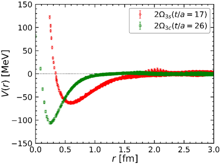
Figure 1: (Color online). The one-dimensional projection of the LO potential in the $A_{1}$-rep, $V(r)\equiv\left.V({\bm{r}})\right|_{r=|{\bm{r}}|}$, for $2\Omega_{3s}$ Gongyo et al. (2018) at Euclidean time $t/a=17$ (red circles), and for $2\Omega_{3c}$ Lyu et al. (2021) at Euclidean time $t/a=26$ (green squares).

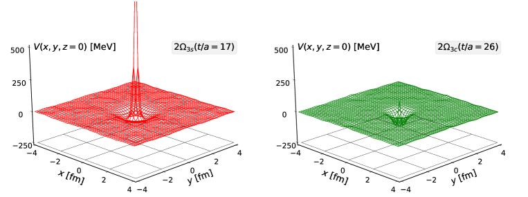
Figure 2: (Color online). The LO potential $V(x,y,z=0)$ in the $A_{1}$-rep for $2\Omega_{3s}$ Gongyo et al. (2018) at Euclidean time $t/a=17$ (left), and for $2\Omega_{3c}$ Lyu et al. (2021) at Euclidean time $t/a=26$ (right).

In Fig. 1, we show the one-dimensional projection of the LO potential on the three-dimensional lattice box, $V(r)\equiv\left.V({\bm{r}})\right|_{r=|{\bm{r}}|}$, obtained by the time-dependent HAL QCD method in the $A_{1}$ representation of the cubic group $SO(3,\mathbb{Z})$ ($A_{1}$-rep in short) for $2\Omega_{3s}$ Gongyo et al. (2018) at $t/a=17$, and for $2\Omega_{3c}$ Lyu et al. (2021) at $t/a=26$. These Euclidean times are chosen such that they are large enough to suppress contaminations from excited states in the single-baryon correlator and simultaneously small enough to avoid exponentially increasing statistical errors. The potential for $2\Omega_{3c}$ is shorter ranged with smaller repulsive core than that for $2\Omega_{3s}$. In both systems, the LO potentials $V({\bm{r}})$ are localized around the origin and are approximately spherical functions as shown in Fig. 2 for $V(x,y,z=0)$. Also, $V(r)$ in Fig. 1 can be well-fitted by the three-range Gaussians, $V_{\rm fit}(r)=\sum_{i=1,2,3}\alpha_{i}\exp(-\beta_{i}r^{2})$ Gongyo et al. (2018); Lyu et al. (2021). Due to the large cancellation between the medium-range attraction and the short-range repulsion, only one loosely bound state appears in the infinite volume ($L=\infty$) for each of $2\Omega_{3s}$ Gongyo et al. (2018) and $2\Omega_{3c}$ Lyu et al. (2021).

V.1 Eigenfunctions of $H_{\rm LO}$ on the lattice

Using the LO potential $V({\bm{r}})$, the discretized Hamiltonian $H_{\rm LO}\equiv H_{0}+V$ can be diagonalized on the three-dimensional lattice box with the size $(La)^{3}\simeq(8.1{\rm fm})^{3}$ and $L=96$. Under the periodic boundary condition, we thus obtain the eigenenergies $\Delta E_{n}$ and associated eigenfunctions $\psi_{n}(\bm{r})$ in the $A_{1}$-rep. Note that $\psi_{n}$ here represents an approximation of the exact $n$-th NBS wave function $\Psi_{E_{n}}$ associated with the LO potential $V$ as discussed in Sec. III. The eigenfunctions are normalized $\sum_{\bm{r}}|\psi_{n}(\bm{r})|^{2}=1$ with a convention $\psi_{n}(\bm{0})>0$. Shown in Fig. 3 are the first four states $(n=0,1,2,3)$, $\psi_{n}(x,y,z=0)$, together with $\Delta E_{n}$. The eigenfunctions are distorted by the boundary condition and have only discrete rotational symmetry. Therefore those in the $A_{1}$-rep not only contain component with angular momentum $l=0$ but also components with $l=4,6,\cdots$. Such a mixing becomes prominent as $r$ and/or $n$ increase.

Shown in Fig. 4 are the one-dimensional projection of the above eigenfunctions, $\psi_{n}(r)\equiv\left.\psi_{n}({\bm{r}})\right|_{r=|{\bm{r}}|}$ on the three-dimensional lattice box. Note that the number of nodes of $\psi_{n}(r)$ is equal to $n$ as expected from the quantization condition given by the periodic boundary condition. The characteristic size of the ground state is smaller for the $2\Omega_{3c}$ than that for $2\Omega_{3s}$. Shown together by the black solid lines are the bound-state eigenfunctions $\psi_{\rm inf.}(r)$ in the infinite ($L=\infty$) and continuous ($a=0$) space obtained by solving the Schrödinger equation with $H^{\infty}_{\rm LO}=-\nabla^{2}/m_{\Omega}+V_{\rm fit}(r)$. We find that $\psi_{\rm inf.}(r)$ and $\psi_{0}(r)$ are indistinguishable for $r<3$ fm in both cases.

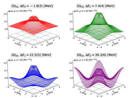
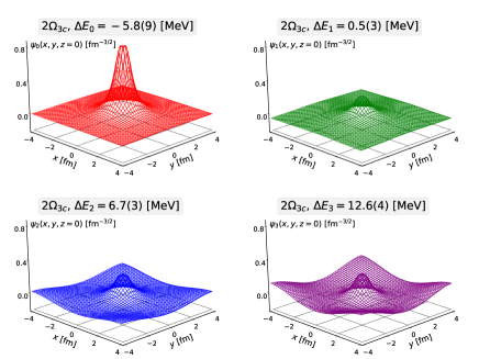
Figure 3: (Color online). The first four eigenfunctions $\psi_{n}(x,y,z=0)$ of the LO Hamiltonian $H_{\rm LO}$ in the $A_{1}$-rep for $2\Omega_{3s}$ (upper four panels) and for $2\Omega_{3c}$ (lower four panels). They are normalized as $\sum_{\bm{r}}|\psi_{n}(\bm{r})|^{2}=1$ with a convention $\psi_{n}(\bm{0})>0$. The red, green, blue, and purple wireframes correspond to $\psi_{n}(x,y,z=0)$ with $n=0$, $1$, $2$, and $3$, respectively. The corresponding eigenenergy $\Delta E_{n}$ is shown at the top of each panel.

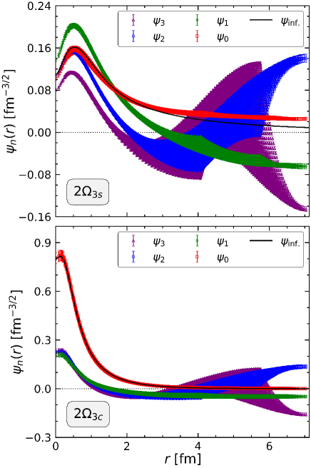
Figure 4: (Color online). The one-dimensional projection of eigenfunctions of $H_{\rm LO}$ in the $A_{1}$-rep on the three-dimensional lattice box, $\psi_{n}(r)\equiv\left.\psi_{n}(\bm{r})\right|_{r=|\bm{r}|}$ for $2\Omega_{3s}$ (upper panel) and for $2\Omega_{3c}$ (lower panel). The red squares, green diamonds, blue circles, and purple triangles correspond to $\psi_{n}(r)$ with $n=0$, $1$, $2$, and $3$ , respectively. The black solid lines are the bound-state wavefunctions $\psi_{\mathrm{inf.}}(r)$ in the infinite and continuum space obtained by solving the Schrödinger equation with $V_{\rm fit}(r)$.

V.2 Effective energies on the lattice

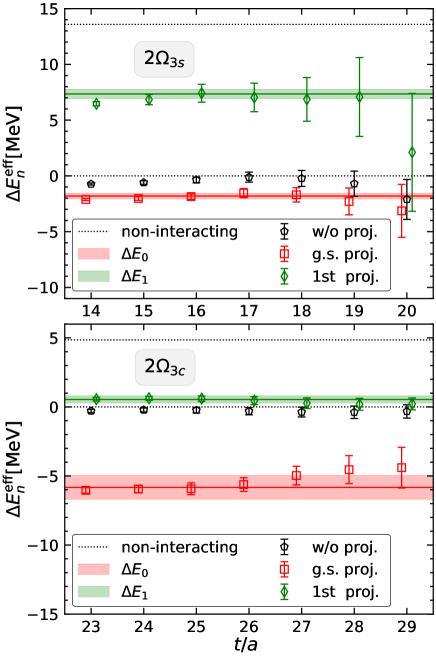
Figure 5: (Color online). The effective energies $\Delta E^{\mathrm{eff}}_{n}(t)$ in Eq. (11) obtained from the projected temporal correlators $R_{n}(t)$ with $n=0$ (red squares) and $1$ (green diamonds) for $2\Omega_{3s}$ (upper panel) and for $2\Omega_{3c}$ (lower panel). The red (green) bands show $\Delta E_{0}$ ($\Delta E_{1}$) calculated from the LO Hamiltonian $H_{\rm LO}$, while the black dotted lines are $\Delta E_{0,1}$ for a non-interacting system. The black pentagons represent the effective energies extracted from the temporal correlations without projection, $R(t)=\sum_{\bm{r}}R(\bm{r},t)$.

Let us now utilize the eigenfunctions $\psi_{n}({\bm{r}})$ to define optimized two-baryon sink operators $S_{n}(t)$ in Eq.(9) and evaluate temporal correlators $R_{n}(t)$ in Eq.(10) to derive the effective energy $\Delta E^{\mathrm{eff}}_{n}(t)$. Shown in Fig. 5 by the open squares and open diamonds as a function of $t/a$ are $\Delta E^{\mathrm{eff}}_{n}(t)$ for $n=0$ and $1$, respectively. To be consistent with the Euclidean time employed to extract $V({\bm{r}})$, we choose $t/a=17\pm 3$ ($26\pm 3$) for $2\Omega_{3s}$ ($2\Omega_{3c}$). The colored bands in Fig. 5 are $\Delta E_{n}$ obtained from $H_{\rm LO}$ as discussed in Sec.V.1. Open pentagons are the “naive” ground-state energy, $\widetilde{\Delta E}(t)=\frac{1}{a}\ln\frac{R(t)}{R(t+1)},$ obtained from the unprojected temporal correlations, $R(t)=\sum_{\bm{r}}R(\bm{r},t)$.

By comparing $\Delta E^{\mathrm{eff}}_{n}(t)$, $\Delta E_{n}$ and $\widetilde{\Delta E}(t)$ in Fig. 5, we find the following points:

• Each effective energy ($\Delta E^{\mathrm{eff}}_{0}(t)$ and $\Delta E^{\mathrm{eff}}_{1}(t)$) has its own plateau for both $2\Omega_{3s}$ and $2\Omega_{3c}$. In addition, good agreements between $\Delta E^{\mathrm{eff}}_{0,1}(t)$ and $\Delta E_{0,1}(t)$ are found.

• The above observations indicate that different eigenstates are properly separated by the projection, and the uncertainty from the derivative expansion of $U$ is within the statistical errors. Otherwise, eigenfunctions $\psi_{0,1}({\bm{r})}$ obtained from $V$ would be different from the exact NBS wave functions $\Psi_{E_{0,1}}({\bm{r}})$.

• Although $\widetilde{\Delta E}(t)$ looks stable, its magnitude does not agree with the ground state energy $\Delta E_{0}$. This is the typical “fake plateaux” behavior due to the contamination from the excited states in $R(t)$. This phenomenon for two-baryon systems was extensively studies in Refs. Iritani et al. (2016, 2017, 2019a).

The same analyses for $n=2$ and $3$ are given in Appendix A where the agreement between $\Delta E^{\mathrm{eff}}_{n}(t)$ and $\Delta E_{n}$ is also observed within the statistical errors.

V.3 Overlapping factors

The coefficients $a_{n}$ in Eq.(10) and $b_{n}$ in Eq.(12) represent the overlapping strengths of the projected and unprojected sink operators to the state created by wall-type source, respectively. By using the eigenfunctions obtained in Sec. V.1, these coefficients can be calculated as $a_{n}=\sum_{{\bm{r}}}\psi^{\dagger}_{n}({\bm{r}})R({\bm{r}},t)e^{(\Delta E_{n})t}$ and $b_{n}=a_{n}\sum_{{\bm{r}}}\psi_{n}({\bm{r}})$ Iritani et al. (2019a). Note that the source and sink operators are not Hermitian conjugate with each other, so that the overlapping coefficients are not necessarily positive. To see the relative magnitude of the coefficients, we plot $|a_{n}/a_{0}|$ and $|b_{n}/b_{0}|$ versus $\Delta E_{n}$ in Fig. 6. These ratios for $2\Omega_{3s}$ ($2\Omega_{3c}$) are evaluated at the center of the plateau, $t/a=17$ ($t/a=26$), in Fig. 5.

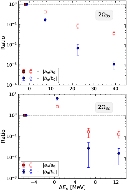
Figure 6: (Color online). The ratio $|a_{n}/a_{0}|$ (red squares) and $|b_{n}/b_{0}|$ (blue circles) with $n=0$, 1, 2, and 3 as functions of $\Delta E_{n}$ for both $2\Omega_{3s}$ (upper panel) and $2\Omega_{3c}$ (lower panel). The solid (open) symbols show the positive (negative) sign for the ratio.

From the red squares for $2\Omega_{3s}$ in Fig. 6, one finds that the wall-type source couples primarily to the $n=0$ state, secondly to the $n=1$ state with $|a_{1}/a_{0}|\simeq 0.4$, and negligibly to the higher states $|a_{2,3}/a_{0}|<0.1$. On the other hand, the red squares for $2\Omega_{3c}$ indicate that the wall-type source couples primarily to the $n=1$ state with $|a_{1}/a_{0}|\simeq 3$. This is due to the fact that the size of the $n=0$ state for $2\Omega_{3c}$ is rather small, so that its coupling to the extended wall-type source is weak. As we mentioned in Sec. II, the advantage of the HAL QCD method is that the decomposition of $R({\bm{r}},t)$ into each eigenstate is not required to derive the potential, since the potential is independent of $n$ as long as the system is in the elastic region. Present results show that the interaction potentials can be extracted reliably in the time-dependent HAL QCD method with the derivative expansion for both $2\Omega_{3s}$ and $2\Omega_{3c}$, regardless whether the ground state or the (first) excited state dominates the two-baryon correlation function.

Let us now turn to the discussion on the unprojected temporal correlation $R(t)$ which produces the fake plateau, i.e. the black pentagons in Fig. 5. From $|b_{1}/b_{0}|$ in Fig. 6, one may evaluate the value of $t/a$ above which the true ground state saturation is reached by $\widetilde{\Delta E}(t)$. Let us demand the systematic error in the effective energy due to the first excited state contamination is bounded, $\left|\frac{\widetilde{\Delta E}(t)-\Delta E_{0}}{\Delta E_{0}}\right|<\varepsilon$. Utilizing $\widetilde{\Delta E}(t)=\ln\frac{R(t)}{R(t+1)}$ with $R(t)=\sum_{i=0,1}b_{i}e^{-(\Delta E_{i})t}$, the above condition gives $t>\frac{1}{\Delta E_{1}-\Delta E_{0}}\ln\left[\frac{b_{1}}{b_{0}}\frac{1-e^{(1-\varepsilon)(\Delta E_{0})-\Delta E_{1}}}{-1+e^{-\varepsilon(\Delta E_{0})}}\right]$ in the case of $b_{1}/b_{0}>0$ and $\Delta E_{0}<0$. Taking $\varepsilon=0.1$ and using $\Delta E_{0,1}$ in Fig. 3, and $b_{1}/b_{0}\simeq 0.2$ ($6$) for $2\Omega_{3s}$ ($2\Omega_{3c}$), we need to have $t/a>580$ for $2\Omega_{3s}$ and $t/a>1500$ for $2\Omega_{3c}$, respectively. However, $R(t)$ for such large $t$ would suffer from exponentially large statistical errors Lepage (1990).

VI Summary and concluding remarks

In this paper, we explored the idea of the optimized interpolating operators originally proposed in Iritani et al. (2019a) on the basis of the time dependent HAL QCD method. To reduce the statistical errors, we considered heavy dibaryons $\Omega_{3Q}\Omega_{3Q}$ ($Q=s,c$) in the ${}^{1}S_{0}$ channel and extracted the leading-order HAL QCD potential $V({\bm{r}})$ localized in space. It was then used to obtain the eigenfunctions and eigenenergies on a finite lattice box with the periodic boundary condition. The eigenfunctions $\psi_{n}(\bm{r})$ were then used to construct the projected two-baryon sink operators $S_{n}(t)$ such that they couple predominantly to each $n$-th state. The temporal correlations $R_{n}(t)$ with such optimized sink operators are used to extract corresponding effective energies $\Delta E^{\text{eff}}_{n}(t)$ which were found to have plateau structure for each $n$. Moreover, they agree quantitatively with $\Delta E_{n}$ calculated by solving the Schrödinger equation on the lattice with $V({\bm{r}})$. Such a feature provides an indirect evidence that the leading-order potential $V$ is a good approximation of the non-local potential $U$ for $2\Omega_{3Q}$ systems within the statistical errors. It also implies that the baryon-baryon interaction potential can be reliably extracted from the time-dependent HAL QCD method, no matter whether the two-baryon correlation function is dominated by the ground state or the (first) excited state, while the analysis of the unprojected temporal correlation $R(t)$ leads to a wrong effective energy associated with a fake plateau.

Although we applied our projection only to the sink operators in this paper, one may apply the idea to the source operators as well to further improve the stability and accuracy of $\Delta E^{\rm eff}_{n}(t)$. Such an approach can also provide an optimized operator basis ($S_{n}$) for the conventional variational method Luscher and Wolff (1990) to study hadron-hadron interactions through the matrix correlation, $C_{nn^{\prime}}(t)=\langle 0|S_{n}(t)S_{n^{\prime}}^{\dagger}(0)|0\rangle$. Further Investigation along this line will be reported elsehwhere.

Appendix A $n=2$ and $3$ cases

Here we show the same analyses along the line with the main text for higher excited states.

Fig. 7 shows the effective energies $\Delta E^{\mathrm{eff}}_{n}(t)$ obtained from the projected temporal correlators $R_{n}(t)$ with $n=2$ (red square) and $n=3$ (green diamond) for both $2\Omega_{3s}$ and $2\Omega_{3c}$. The colored bands are corresponding $\Delta E_{n}$ calculated from the LO Hamiltonian $H_{\rm LO}$. The black pentagons are effective energies obtained from the unprojected temporal correlators. $\Delta E^{\mathrm{eff}}_{2,3}(t)$ are found to be consistent with $\Delta E_{2,3}$. Large statistical errors in $\Delta E^{\mathrm{eff}}_{2,3}(t)$ are due to the fact that the contributions to $R(\bm{r},t)$ from the second and third excited states are very small, as we can see in Fig. 6.

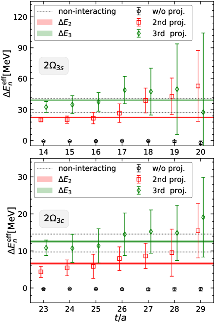
Figure 7: (Color online). The same as Fig. 5, but for $n=2$ and $3$.

References

- Drischler et al. (2021) C. Drischler, W. Haxton, K. McElvain, E. Mereghetti, A. Nicholson, P. Vranas, and A. Walker-Loud, Prog. Part. Nucl. Phys. 121, 103888 (2021), arXiv:1910.07961 [nucl-th] .
- Aoki and Doi (2020) S. Aoki and T. Doi, Frontiers in Physics 8, 307 (2020).
- Luscher (1991) M. Luscher, Nucl. Phys. B 354, 531 (1991).
- Ishii et al. (2007) N. Ishii, S. Aoki, and T. Hatsuda, Phys. Rev. Lett. 99, 022001 (2007).
- Aoki et al. (2010) S. Aoki, T. Hatsuda, and N. Ishii, Prog. Theor. Phys. 123, 89 (2010), arXiv:0909.5585 [hep-lat] .
- Ishii et al. (2012) N. Ishii, S. Aoki, T. Doi, T. Hatsuda, Y. Ikeda, T. Inoue, K. Murano, H. Nemura, and K. Sasaki (HAL QCD Collaboration), Physics Letters B 712, 437 (2012).
- Lepage (1990) G. P. Lepage, in From Actions to Answers: Proceedings of the TASI 1989, edited by T. Degrand and D. Toussaint (World Scientific, Singapore, 1990).
- Iritani et al. (2016) T. Iritani et al., JHEP 10, 101 (2016), arXiv:1607.06371 [hep-lat] .
- Iritani et al. (2019a) T. Iritani, S. Aoki, T. Doi, T. Hatsuda, Y. Ikeda, T. Inoue, N. Ishii, H. Nemura, and K. Sasaki (HAL QCD), JHEP 03, 007 (2019a), arXiv:1812.08539 [hep-lat] .
- Francis et al. (2019) A. Francis, J. R. Green, P. M. Junnarkar, C. Miao, T. D. Rae, and H. Wittig, Phys. Rev. D 99, 074505 (2019), arXiv:1805.03966 [hep-lat] .
- Hörz et al. (2021) B. Hörz et al., Phys. Rev. C 103, 014003 (2021), arXiv:2009.11825 [hep-lat] .
- Amarasinghe et al. (2021) S. Amarasinghe, R. Baghdadi, Z. Davoudi, W. Detmold, M. Illa, A. Parreno, A. V. Pochinsky, P. E. Shanahan, and M. L. Wagman, (2021), arXiv:2108.10835 [hep-lat] .
- Gongyo et al. (2018) S. Gongyo, K. Sasaki, S. Aoki, T. Doi, T. Hatsuda, Y. Ikeda, T. Inoue, T. Iritani, N. Ishii, T. Miyamoto, and H. Nemura (HAL QCD), Phys. Rev. Lett. 120, 212001 (2018).
- Lyu et al. (2021) Y. Lyu, H. Tong, T. Sugiura, S. Aoki, T. Doi, T. Hatsuda, J. Meng, and T. Miyamoto, Phys. Rev. Lett. 127, 072003 (2021), arXiv:2102.00181 [hep-lat] .
- Zimmermann (1987) W. Zimmermann, in Wondering in the fields: Festschrift for Prof. K. Nishijima, edited by K. Kawarabayashi and A. Ukawa (World Scientific, Singapore, 1987).
- Aoki et al. (2013) S. Aoki, B. Charron, T. Doi, T. Hatsuda, T. Inoue, and N. Ishii, Phys. Rev. D 87, 034512 (2013), arXiv:1212.4896 [hep-lat] .
- Iritani et al. (2019b) T. Iritani, S. Aoki, T. Doi, S. Gongyo, T. Hatsuda, Y. Ikeda, T. Inoue, N. Ishii, H. Nemura, and K. Sasaki (HAL QCD), Phys. Rev. D 99, 014514 (2019b), arXiv:1805.02365 [hep-lat] .
- Umeda et al. (2001) T. Umeda, R. Katayama, O. Miyamura, and H. Matsufuru, Int. J. Mod. Phys. A 16, 2215 (2001), arXiv:hep-lat/0011085 .
- Larsen et al. (2020) R. Larsen, S. Meinel, S. Mukherjee, and P. Petreczky, Phys. Lett. B 800, 135119 (2020), arXiv:1910.07374 [hep-lat] .
- Chen et al. (2021) F. Chen, X. Jiang, Y. Chen, K.-F. Liu, W. Sun, and Y.-B. Yang, (2021), arXiv:2111.11929 [hep-lat] .
- Iritani et al. (2017) T. Iritani, S. Aoki, T. Doi, T. Hatsuda, Y. Ikeda, T. Inoue, N. Ishii, H. Nemura, and K. Sasaki, Phys. Rev. D 96, 034521 (2017), arXiv:1703.07210 [hep-lat] .
- Ishikawa et al. (2016) K.-I. Ishikawa, N. Ishizuka, Y. Kuramashi, Y. Nakamura, Y. Namekawa, Y. Taniguchi, N. Ukita, T. Yamazaki, and T. Yoshie (PACS), Proc. Sci. LATTICE2015, 075 (2016), arXiv:1511.09222 [hep-lat] .
- Aoki et al. (2003) S. Aoki, Y. Kuramashi, and S.-i. Tominaga, Prog. Theor. Phys. 109, 383 (2003), arXiv:hep-lat/0107009 .
- Namekawa (2017) Y. Namekawa (PACS), Proc. Sci. LATTICE2016, 125 (2017).
- Doi and Endres (2013) T. Doi and M. G. Endres, Comput. Phys. Commun. 184, 117 (2013), arXiv:1205.0585 [hep-lat] .
- Luscher and Wolff (1990) M. Luscher and U. Wolff, Nucl. Phys. B 339, 222 (1990).
- (27) http://www.lqcd.org/ildg and http://www.jldg.org.