Categorical Hopfield Networks

Abstract.

This paper discusses a simple and explicit toy-model example of the categorical Hopfield equations introduced in previous work of Manin and the author. These describe dynamical assignments of resources to networks, where resources are objects in unital symmetric monoidal categories and assignments are realized by summing functors. The special case discussed here is based on computational resources (computational models of neurons) as objects in a category of deep neural networks (DNN), with a simple choice of the endofunctors defining the Hopfield equations that reproduce the usual updating of the weights in DNNs by gradient descent.

1. Introduction: categorical Hopfield equations

In [17] a categorical model of neuronal networks with assigned resources was developed based on Segal’s formalism [23] of categories of summing functors and Gamma-spaces, see also [18], [19]. Resources are modeled according to [6], as categories ${\mathcal{C}}$ endowed with either a unital symmetric monoidal structure, or in a more restrictive case categories with a coproduct (categorical sum) and zero-object (both initial and terminal). Given a finite set $X$, summing functors $\Phi$ are assignments of resources, that is objects in ${\mathcal{C}}$, to subsets of $X$ that are additive (in the coproduct or the monoidal operation of ${\mathcal{C}}$) over disjoint subsets.

In this model, the category $\Sigma_{\mathcal{C}}(X)$ of summing functors and invertible natural transformations introduced in [23] is viewed as the parameterizing space of all possible such assignments of ${\mathcal{C}}$-resources up to equivalence. Instead of considering just a finite set $X$, one can consider a network (finite directed graph) $G$ and summing functors $\Phi$ that assign ${\mathcal{C}}$-resources to subnetworks $G^{\prime}\subset G$, with a corresponding category $\Sigma_{\mathcal{C}}(G)$ of network summing functors. The category $\Sigma_{\mathcal{C}}(G)$ (or a suitable subcategory representing additional constraints on the summing functors such as conservation laws at vertices, inclusion-exclusion, or other compositional properties) is considered as the “configuration space” of the model.

A dynamical system is then introduced on this configuration space, in the form of an equation modeled on the Hopfield equations of network dynamics. Here the variable of the equation is a summing functor (an assignment of resources) and the dynamics is determined by an initial condition (an initial assignment) and endofunctors of the category of resources that determine the dynamics and play a role analogous to the matrix of weights in the usual Hopfield equations (which we review in §1.2 below).

The setting presented in [17] is quite abstract and involves choices of a category of resources ${\mathcal{C}}$, a suitable subcategory of network summing functors $\Sigma_{\mathcal{C}}(G)$, and a collection of endofunctors of ${\mathcal{C}}$ that determine the Hopfield dynamics. We summarize in §1.1 and §1.3 the notion of network summing functors and the categorical Hopfield equations introduced in [17]. The main idea is to replace the variables of the classical Hopfield equations, which describe firing activity and firing rates of neurons, with variables that describe assignments of resources of a certain type to the nodes (and/or edges) of a network, so that the equations can be used to describe how these assignments evolve in time, under specific transformation of both the network and the associated resources. The purpose of the present paper is to illustrate this mechanism in a more concrete setting, with a specific choice of a category ${\mathcal{C}}$ of computational models of the nodes of the network, motivated by computational models of the neuron via deep neural networks developed in [2].

The categorical Hopfield equations we discuss as our main example in this paper should not be regarded as a realistic model of categorical dynamics for a neuronal network, rather it is designed to be just a simple toy model where the categorical setting is easy to describe and properties of the resulting equations can be easily identified.

The main results presented in this paper consist of: the construction of a category of resources based on deep neural networks (DNNs); the explicit form of the categorical Hopfield equations with this category of resources, in the cases with or without a leak-term in the equations; the analysis of fixed points of these equations and the identification of the backpropagation mechanism for the weights of DNNs based on gradient descent as a special case of this categorical Hopfield dynamics.

1.1. Resources and summing functors

The mathematical theory of resources and resource convertibility developed in [6] and [9] describes resources as objects in a unital symmetric monoidal category ${\mathcal{C}}$, with the unit representing the empty resource and the monoidal operation describing the combination of independent resources. Convertibility between resources $A$ and $B$ is described by the existence of a nonempty set of morphisms, ${\rm Mor}_{\mathcal{C}}(A,B)\neq\emptyset$. A measure of the convertibility of resources is provided by the preordered abelian semigroup given by the set of isomorphism classes $[A]$ of objects $A$ in ${\mathcal{C}}$ with the operation $[A]+[B]=[A\oplus B]$ with $\oplus$ the monoidal structure of ${\mathcal{C}}$, and with $[A]\succeq[B]$ whenever convertibility from $A$ to $B$ holds, namely whenever ${\rm Mor}_{\mathcal{C}}(A,B)\neq\emptyset$.

The notion of summing functors was introduced by Segal in [23] as part of the mechanism of Gamma-spaces, a homotopy theoretic construction of spectra from categories with certain properties (sums and zero-object in Segal’s original formulation, or unital symmetric monoidal categories in the more general formulation of Thomason, [21], [22]). Summing functors are assignments $\Phi$ of objects in a category ${\mathcal{C}}$ of resources to subsets of a given finite set $X$, that are additive on disjoint subsets (with respect to the monoidal structure $\oplus$ of ${\mathcal{C}}$),

(1.1) $$\Phi(X_{1}\sqcup X_{2})=\Phi(X_{1})\oplus\Phi(X_{2}),$$

with $\Phi(\emptyset)=0$, that are functorial under inclusions of subsets of $X$. Morphisms in the category of summing functors are invertible natural transformations. Summing functors are completely determined by the collection of objects $\{\Phi(x)\}_{x\in X}$ in ${\mathcal{C}}$ and invertible natural transformations of summing functors by isomorphisms $\{\eta_{x}\}_{x\in X}$ of these objects. This identifies the category $\Sigma_{\mathcal{C}}(X)$ of ${\mathcal{C}}$-valued summing functors on a given finite set $X$ of cardinality $n$ with the $n$-fold cartesian product $\hat{\mathcal{C}}^{n}$ of the category $\hat{\mathcal{C}}$ with the same objects as ${\mathcal{C}}$ and the isomorphisms of ${\mathcal{C}}$ as morphisms.

This simple notion of summing functors can be generalized in various ways when the finite set $X$ is replaced by a finite directed graph $G$. The resulting categories of “network summing functors” are described in [17].

We focus here on one particular case among those described in [17], namely the case where the network summing functors are compatible with a compositional structure on the category of resources described by an operad or a properad. We need to recall the setting we consider on the category of resources before introducing the appropriate notion of network summing functors.

1.1.1. Properads and operads in categories

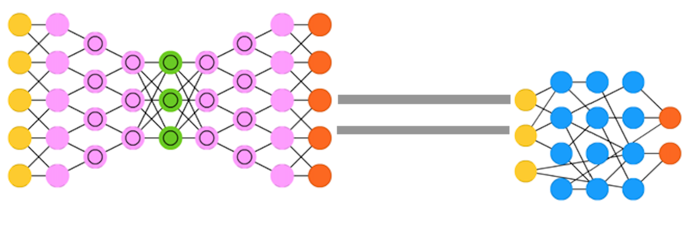
Figure 1. Example of properad composition $\circ^{3,4}_{1,2}:{\mathcal{P}}(5,5)\times{\mathcal{P}}(3,2)\to{\mathcal{P}}(6,5)$ connecting the third and fourth outputs of the first object (machine) to the first and second inputs of the second one. The inputs of the resulting object (machine) are the inputs of the first one and the remaining inputs of the second, and the resulting outputs are the outputs of the second together with the remaining outputs of the first.

Let Cat denote the category of small categories. A properad in Cat is a collection ${\mathcal{P}}=\{{\mathcal{P}}(n,m)\}_{n,m\in{\mathbb{N}}}$ of small categories with composition functors

(1.2) $$\circ^{i_{1},\ldots,i_{\ell}}_{j_{1},\ldots,j_{\ell}}:{\mathcal{P}}(m,k)\times{\mathcal{P}}(n,r)\to{\mathcal{P}}(m+n-\ell,k+r-\ell)$$

for subsets $\{i_{1},\ldots,i_{\ell}\}\subset\{1,\ldots,k\}$ and $\{j_{1},\ldots,j_{\ell}\}\subset\{1,\ldots,n\}$ with $i_{s}<i_{s+1}$ and $j_{s}<j_{s+1}$ for $s=1,\ldots,\ell-1$. These composition operations satisfy associativity axioms and unity axioms (see [14], [20], [24]). The properad is symmetric if, moreover, there is an action of $\Sigma_{n}\times\Sigma_{m}$ on ${\mathcal{P}}(n,m)$ with respect to which the composition maps are bi-equivariant.

We think of the objects in ${\mathcal{P}}(n,m)$, in a properad ${\mathcal{P}}$, as computational architectures with $n$ inputs and $m$ outputs, with the composition operations $\circ^{i_{1},\ldots,i_{\ell}}_{j_{1},\ldots,j_{\ell}}$ that graft the subset of outputs $\{i_{1},\ldots,i_{\ell}\}$ of the first machine to the subset of inputs $\{j_{1},\ldots,j_{\ell}\}$ of the second machine, in the given order, see Figure 1. In the special case where we restrict to computational architectures with a single output, we obtain the case of an operad. One can also consider non-symmetric properads and operads (namely without the condition of equivariance with respect to the symmetric group actions). Indeed, we will focus on examples that are non-symmetric. Thus, in the following, when we refer to operads and properads, we will not assume the symmetric condition unless explicitly stated.

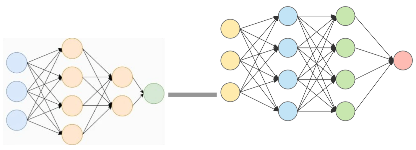
Figure 2. Example of operad composition $\circ_{3}:{\mathcal{O}}(3)\times{\mathcal{O}}(3)\to{\mathcal{O}}(5)$ connecting the single output of the first object (machine) to the third input of the second one. The inputs of the resulting object (machine) are the inputs of the first one together with the remaining inputs of the second.

An operad in Cat is a collection ${\mathcal{O}}=\{{\mathcal{O}}(n)\}_{n\in{\mathbb{N}}}$ of small categories with composition functors

(1.3) $$\circ_{j}:{\mathcal{O}}(m)\times{\mathcal{O}}(n)\to{\mathcal{O}}(m+n-1),$$

subject to associativity, unity, and symmetry constraints as above.

In the case if a symmetric operad one also requires the existence of actions of $\Sigma_{n}$ on ${\mathcal{O}}(n)$ with respect to which the composition maps are equivariant.

In the case of operads, the objects of ${\mathcal{O}}(n)$ have $n$ inputs and one output and the composition operation $\circ_{j}$ connects the output of the first machine to the $j$-th input of the second, thus giving a new machine with $n+m-1$ inputs and a single output, see Figure 2.

In particular we say that a unital symmetric monoidal category ${\mathcal{C}}$ carries a properad structure when there is a family of full subcategories ${\mathcal{C}}(n,m)$ for $n,m\in{\mathbb{N}}$ with the properties:

• ${\rm Obj}({\mathcal{C}})=\sqcup_{n,m\in{\mathbb{N}}}{\rm Obj}({\mathcal{C}}(n,m))$;

• the monoidal structure $(\otimes,{\mathbb{I}})$ satisfies

  (1.4) $$\otimes:{\mathcal{C}}(m,k)\times{\mathcal{C}}(n,r)\to{\mathcal{C}}(m+n,k+r)\,;$$

• the family $\{{\mathcal{C}}(n,m)\}_{n,m\in{\mathbb{N}}}$ is a properad in ${\rm Cat}$.

It is customary to also require additional compatibility conditions between the monoidal structure and the properad structure. For instance, in the properad case we can consider compatibility conditions of the form

(1.5) $$(A\otimes B)\circ^{{\mathcal{I}}\sqcup{\mathcal{I}}^{\prime}}_{{\mathcal{J}}\sqcup{\mathcal{J}}^{\prime}}(C\otimes D)=(A\circ^{\mathcal{I}}_{\mathcal{J}}C)\otimes(B\circ^{{\mathcal{I}}^{\prime}}_{{\mathcal{J}}^{\prime}}D)\,,$$

for $A\in{\mathcal{P}}(m,k)$, $C\in{\mathcal{P}}(n,r)$, $B\in{\mathcal{P}}(m^{\prime},k^{\prime})$ and $D\in{\mathcal{P}}(n^{\prime},r^{\prime})$ and with ${\mathcal{I}}=\{i_{1},\ldots,i_{\ell}\}\subset\{1,\ldots,k\}$, ${\mathcal{J}}=\{j_{1},\ldots,j_{\ell}\}\subset\{1,\ldots,n\}$, ${\mathcal{I}}^{\prime}=\{i^{\prime}_{1},\ldots,i^{\prime}_{\ell^{\prime}}\}\subset\{1,\ldots,k^{\prime}\}$, ${\mathcal{J}}^{\prime}=\{j^{\prime}_{1},\ldots,j^{\prime}_{\ell^{\prime}}\}\subset\{1,\ldots,n^{\prime}\}$. Here the “$=$” sign in (1.5) should in general indicate isomorphism in the category ${\mathcal{P}}$ rather than strict equality.

We will discuss in §2.1.2 an example where compatibility conditions of the form (1.5) hold.

In the case of an operad structure we similarly have the following setting.

Let ${\mathcal{C}}$ be a symmetric monoidal category with full subcategories ${\mathcal{C}}(n)$ for $n\in{\mathbb{Z}}_{\geq 0}={\mathbb{N}}\cup\{0\}$ with the following properties:

• ${\rm Obj}({\mathcal{C}})=\sqcup_{n\in{\mathbb{Z}}_{\geq 0}}{\rm Obj}({\mathcal{C}}(n))$;

• the $\{{\mathcal{C}}(n)\}_{n\in{\mathbb{N}}}$ form an operad in ${\rm Cat}$ with unital associative composition functors

  $$\circ_{j}:{\mathcal{C}}(m)\times{\mathcal{C}}(n)\to{\mathcal{C}}(m+n-1)\,;$$

• ${\mathcal{C}}(0)=\{{\mathbb{I}}\}$, with ${\mathbb{I}}$ the unit of the monoidal structure $(\otimes,{\mathbb{I}})$, and for all $n,m\in{\mathbb{Z}}_{\geq 0}$

  (1.6) $$\otimes:{\mathcal{C}}(n)\otimes{\mathcal{C}}(m)\to{\mathcal{C}}(n+m)\,.$$

First observe that if the operad structure on the ${\mathcal{C}}(n)$ is induced from a properad by taking the single-output ${\mathcal{P}}(n,1)$, the monoidal structure (1.6) necessarily differs from the monoidal structure (1.4), which would instead give

(1.7) $$\otimes:{\mathcal{P}}(n,1)\times{\mathcal{P}}(m,1)\to{\mathcal{P}}(n+m,2)\,.$$

Indeed, in specific cases (like the one we will be discussing in §2.1.3 below) one can obtain a monoidal structure satisfying (1.6) from (1.4) using the monoidal structure of (1.7) followed by an “identification of the two outputs” in (1.6). We will discuss this more explicitly in §2.1.3.

Note that in this case the compatibility conditions between the monoidal structure and the prooperad composition of (1.5) also do not directly induce compatibility conditions of the same form on the operad. However we do obtain an induced compatibility condition of the form

(1.8) $$A\circ_{j}(C\otimes D)=\left\{\begin{array}[]{ll}(A\circ_{j}C)\otimes D&j=1,\ldots,m\\ C\otimes(A\circ_{j^{\prime}}D)&j^{\prime}=j-m=1,\ldots,k,\end{array}\right.$$

for all $A\in{\mathcal{C}}(m)$, $C\in{\mathcal{C}}(n)$, $D\in{\mathcal{C}}(k)$ with $m,n,k\in{\mathbb{N}}$. Again the “$=$” sign in general denotes isomorphism in the category ${\mathcal{C}}$ rather than strict equality.

This will be useful in the specific example we discuss in §2.1.3 below.

Note that we have the unit of the operad composition, ${\bf 1}\in{\mathcal{C}}(1)$, satisfying ${\bf 1}\circ_{j}A=A=A\circ_{j}{\bf 1}$, for all $A\in{\mathcal{C}}(n)$ and $n\in{\mathbb{N}}$, and the unit of the monoidal structure ${\mathbb{I}}\in{\mathcal{C}}(0)$ satisfying ${\mathbb{I}}\otimes A=A=A\otimes{\mathbb{I}}$, for all $A\in{\mathcal{C}}(n)$ and $n\in{\mathbb{Z}}_{\geq 0}$. In general we do not assume a relation between these two objects, but we will discuss explicitly how they are related in the example we discuss in §2.1.3 below.

1.1.2. Compositional network summing functors

Let ${\mathcal{C}}$ be a category of resources given by a unital symmetric monoidal category with a properad structure $\{{\mathcal{C}}(n,m)\}$ as above. Let $G$ be a finite directed graph. A compositional ${\mathcal{C}}$-valued network summing functor on $G$ consists of an assignment of objects of ${\mathcal{C}}$ to subnetworks of $G$, functorial under inclusions, with the property that the objects $\{\Phi(v)\}_{v\in V(G)}$ of ${\mathcal{C}}$ associated to the vertices of $G$ belong to ${\rm Obj}({\mathcal{C}}(\deg^{in}(v),\deg^{out}(v)))$ with $\deg^{in/out}(v)$ the in and out degrees of the vertex $v$, and that for any $G^{\prime}\subseteq G$ the object $\Phi(G^{\prime})$ is obtained from the objects $\Phi(v)$ for $v\in V(G^{\prime})$ by applying the composition operations $\circ^{i_{1},\ldots,i_{\ell}}_{j_{1},\ldots,j_{\ell}}$ of the properad, as in (1.2), according to the gluing of input and output half-edges of the corollas of the vertices $v\in V(G^{\prime})$ to form the edges of $E(G^{\prime})$. We will return to this definition in more detail in §2.2 below. We will also describe more explicitly notation and assumptions about the networks $G$ in §2.1.1.

We write $\Sigma_{\mathcal{C}}(G)$ for the category of compositional ${\mathcal{C}}$-valued network summing functor on $G$, defined as above, with invertible natural transformations. By the compositional property, the summing functors are completely determined by the objects $\{\Phi(v)\}_{v\in V(G)}$ and the invertible natural transformations by isomorphisms of these objects.

1.2. Hopfield equations and threshold linear networks

The classical Hopfield equations were introduced to model memory storage and retrieval in neuronal networks, adapting ideas from the statistical physics of spin glasses, [12].

In this original form, the variables in the equation are binary $x_{j}=\pm 1$, describing the on/off firing status of individual neurons over a time interval $\Delta t$ of fixed size. The equations take the form

$$x_{i}(n+1)={\rm sign}\left(\sum_{j}W_{ij}x_{j}(n)\right)\,,$$

where $W_{ij}$ is a weight matrix that describes the strength of the connectivity between different neurons. A model of memory storage and retrieval is obtained by choosing a weight matrix determined by a given set of patterns (binary strings $\pi^{a}_{i}$, $a=1,\ldots,M$) one wants to store in the network (Hebbian learning rule)

$$W_{ij}=\frac{1}{N}\sum_{a=1}^{M}\pi^{a}_{i}\pi^{a}_{j}\,.$$

The convergence of the dynamics to the minima of the energy functional

$${\mathcal{E}}=-\sum_{ij}W_{ij}x_{i}x_{j}$$

corresponds to convergence to the stored patterns whenever the input data are sufficiently close to one of the patterns, so that the stored memory can be reconstructed from partial data, see [1], [11] for a more detailed account.

A continuous variables version of the Hopfield equations (see [13]) was developed to model the firing rates of neurons, which are now described by real variables $x_{j}$ in the equations, which take the form

(1.9) $$\frac{dx_{i}}{dt}=-\frac{x_{i}}{\tau}+\sigma\left(\sum_{j}W_{ij}x_{j}+\theta_{i}\right)\,,$$

with a non-linear function $\sigma$ used to ensure that the input firing rates are non-negative. A “bias term” $\theta_{i}$ is also introduced in this form of the equation to model the presence of an external input (an injected current). The first term on the right-hand-side of the equation (1.9) is referred to as “leak term” and is responsible for describing a synaptic current that decays at an exponential rate $\exp(-t/\tau)$. The weight matrix $W_{ij}$ describes the excitatory or inhibitory action (depending on the sign of the matrix entries) of neurons on other neurons, while the leak term describes the inhibitory action of a neuron on itself.

In particular, the non-linearity $\sigma$ can be taken of the threshold-linear form

$$\sigma(x)=(x)_{+}:=\max\{x,0\}.$$

In this case the Hopfield equations (1.9) are also known as “threshold linear networks”.

1.2.1. Inhibitory-excitatory balance

The matrix entries $W_{ij}$ of the weight matrix in (1.9) are real numbers can have either positive or negative sign. This is the reason why one thinks of these equations as the analog of a statistical physics spin glass model rather than an Ising model where the interaction weights are positive and energetically favor spin alignment. The negative and positive signs of the entries $W_{ij}$ here model inhibitory and excitatory interactions between neurons.

Experimental evidence in neuroscience shows that inhibitory and excitatory interactions in the cerebral cortex are well balanced during resting states and during sensory processing, with a balanced condition that occurs either in the form of an overall global balance or a temporal balance. It is shown in [4] that perturbing the global inhibitory-excitatory balance condition in favor of either excitation dominating inhibition or viceversa has significant effects on the behavior of the resulting dynamics, while in [25] it is shown that inhibitory-excitatory balance can emerge from the dynamics (in a mean field theory model) as a stationary state of large networks. Moroever, it is shown in [27] that the inhibitory-excitatory balance condition may be a fundamental mechanism underlying efficient neural coding.

In this paper we show that a global inhibitory-excitatory balance condition arises naturally from the categorical form of the Hopfield equations introduced in [17], imposed by the categorical form of the threshold nonlinearity of the equations. We also show the effects on the dynamics of the violation of the inhibitory-excitatory balance.

1.3. Dynamics in categories of summing functors

In [17] categorical forms of the Hopfield network equations were introduced, motivated by a finite difference version of the classical Hopfield equations. The latter can be written either in the form

(1.10) $$\frac{x_{i}(t+\Delta t)-x_{i}(t)}{\Delta t}=(\sum_{j}W_{ij}x_{j}(t)+\theta_{i})_{+}\,,$$

or with an additional “leak term” $-x_{i}(t)$ as

(1.11) $$\frac{x_{i}(t+\Delta t)-x_{i}(t)}{\Delta t}=-x_{i}(t)+(\sum_{j}W_{ij}x_{j}(t)+\theta_{i})_{+}\,,$$

where the non-linear threshold on the right-hand-side is given by $(\cdot)_{+}=\max\{0,\cdot\}$, and the weight matrix $W_{ij}$ and bias term $\theta_{i}$ are as discussed in §1.2 above. Note that (1.11) is the discretized finite-difference version of the differential equation (1.9) (taken with $\tau=1$).

An analog of these equations is obtained by replacing the real-valued variables $x_{j}(t)$ describing neuron firing rates with variables in the category of network summing functors describing assignments of resources of type ${\mathcal{C}}$ to the network, with the matrix $W$ of weights replaced by a matrix $T$ of endofunctors of the category of resources. The resulting categorical Hopfield network equations proposed in [17] take the form

(1.12) $$X_{v}(n+1)=X_{v}(n)\oplus\left(\oplus_{e\in E\,:\,s(e)=v}T_{e}(X_{t(e)}(n))\oplus\Theta_{v}\right)_{+}$$

or possibly

(1.13) $$X_{v}(n+1)=\left(\oplus_{e\in E\,:\,s(e)=v}T_{e}(X_{t(e)}(n))\oplus\Theta_{v}\right)_{+}\,,$$

We refer to the first case (1.12) as “with leak term” and the second case (1.13) as “without leak term”.

Here the $T_{e}$ for $e\in E(G)$ (or $T_{vv^{\prime}}$ for $v,v^{\prime}\in V(G)$) are a collection of endofunctors of ${\mathcal{C}}$ and $\Theta$ is an assigned summing functor (specified by the objects $\Theta_{v}$ in ${\mathcal{C}}$), while the variables $X_{v}(n)$ of the equation are a sequence of objects $X(n)\in\Sigma_{\mathcal{C}}(G)$, each determined by the objects $\{X_{v}(n)\}_{v\in V}$ of ${\mathcal{C}}$. The nonlinear threshold is now defined in terms of convertibility conditions in the category ${\mathcal{C}}$ of resources, where for $C\in{\rm Obj}({\mathcal{C}})$ we set $(C)_{+}=C$ if $[C]\succeq 0$ and $(C)_{+}=0$ (the unit of the monoidal structure of ${\mathcal{C}}$) otherwise.

The endofunctors $T$ of the category of resources are assumed to preserve the unital symmetric monoidal structure of ${\mathcal{C}}$, although the non-linear threshold does not.

We can also write the equations (1.12) (1.13) above in the form

(1.14) $$\begin{array}[]{rl}X_{v}(n+1)=&X_{v}(n)\oplus\left(\oplus_{v^{\prime}\in V}T_{vv^{\prime}}(X_{v^{\prime}}(n))\oplus\Theta_{v}\right)_{+}\ \ \text{ or }\\ X_{v}(n+1)=&\left(\oplus_{v^{\prime}\in V}T_{vv^{\prime}}(X_{v^{\prime}}(n))\oplus\Theta_{v}\right)_{+}\,,\end{array}$$

where we identify

$$T_{vv^{\prime}}=\oplus_{e\in E\,:\,s(e)=v,\,t(e)=v^{\prime}}T_{e}\,,$$

with the monoidal sum applied pointwise $(\oplus_{e}T_{e})(X):=\oplus_{e}T_{e}(X)$. In the case where the graph does not have multiple edges, $T_{vv^{\prime}}(X_{v^{\prime}})=T_{e}(X_{v^{\prime}})$ if there is an edge between $v$ and $v^{\prime}$ and is $0$ otherwise. Thus, we can use either the form (1.12) and (1.13) or the form (1.14) of the equations.

It it important to note that in equations such as (1.12), (1.13), (1.14), since we are dealing with objects in a category, the “$=$” sign of the equation can be interpreted as the existence of an isomorphism in the given category between the objects in the left-hand-side and the right-hand-side of the equation. In the case of a small category, one can also interpret the “$=$” sign in the equation in the stricter sense of equality rather than isomorphism of objects, but equality in general is not as good a notion in a category theory setting as isomorphism, so it is preferable to interpret the equation as requiring isomorphism. As we discuss briefly in §1.3.1, these two different intepretations of the equations lead to different notions of fixed points and periodic orbits of the dynamics.

In this paper we will discuss these two cases (with and without leak term) and their different behavior in a toy model example with a particular choice of the category ${\mathcal{C}}$ of resources. We write the equations as above, in terms of variables $X_{v}$ at vertices of $G$ rather than edges as in [17] because of our specific choice of category of network summing functors, given by the compositional network summing functors defined above, which are determined by objects of ${\mathcal{C}}$ assigned to vertices rather than edges.

The goal of the present paper is to illustrate more concretely the properties of these categorical Hopfield equations in a specific example motivated by a computational model of neurons developed in [2], with our category ${\mathcal{C}}$ of (computational) resources given by a category of deep neural networks (DNNs).

1.3.1. Fixed points in categories

Before discussing specific examples of the categorical dynamics introduced above, we recall some general facts about fixed points of endofunctors that will be useful in the following.

An important first step in the study of dynamical systems is the structure of fixed points. In a categorical setting like the one we are considering here, this involves discussing fixed points of endofunctors in categories. The same setting can be adapted to study the existence of periodic orbits, as fixed points of powers of the same endofunctor.

Given a category ${\mathcal{C}}$ and an endofunctor $F:{\mathcal{C}}\to{\mathcal{C}}$, a fixed point for $F$ is a pair $(X,\alpha)$ of an object $X\in{\rm Obj}({\mathcal{C}})$ and an isomorphism $\alpha:X\to F(X)$ in ${\rm Mor}_{{\mathcal{C}}}(X,F(X))$.

Fixed points of an endofunctor $F$ of a category ${\mathcal{C}}$ form a category ${\rm Fix}(F)$ with objects the fixed points $(X,\alpha)$ and morphisms in ${\rm Mor}_{{\rm Fix}(F)}((X,\alpha),(Y,\beta))$ given by commutative diagrams

with a morphism $f\in{\rm Mor}_{\mathcal{C}}(X,Y)$. There is a forgetful functor ${\rm Fix}(F)\to{\mathcal{C}}$ that maps $(X,\alpha)\mapsto X$ and a diagram as above to the morphism $f:X\to Y$.

Note that the category ${\rm Fix}(F)$ can be empty if the endofunctor $F$ has no fixed points. An example of an endofunctor with no fixed points is the functor ${\mathcal{P}}:{\rm Sets}\to{\rm Sets}$ with ${\mathcal{P}}(X)=2^{X}$ the power-set functor, since there cannot be a bijection between a set and its set of parts.

A fixed point $(X,\alpha)$ of an endofunctor $F$ on a small category ${\mathcal{C}}$ i s strict if $F(X)=X$ with $\alpha$ the identity morphism. The existence of strict fixed points is in general a much more restrictive condition. However, the following criterion (Proposition 2.6 of [16]) is especially useful: An endofunctor $F:{\mathcal{C}}\to{\mathcal{C}}$ has a strict fixed point $F(X)=X$ if the induced continuous map $|F|:|{\mathcal{N}}{\mathcal{C}}|\to|{\mathcal{N}}{\mathcal{C}}|$ on the topological realization of the nerve ${\mathcal{N}}{\mathcal{C}}$ of the category ${\mathcal{C}}$ has a fixed point.

A point of order $n$ of an endofunctor $F$ is a fixed point of the endofunctor $F^{n}$ that is not a fixed point of any other $F^{k}$ with $k<n$, namely a pair $(X,\gamma)$ of an object $X$ and an isomorphism

$$\gamma:X\stackrel{{\scriptstyle\simeq}}{{\to}}F^{n}(X),$$

, such that $X\not\simeq F^{k}(X)$ for any $k<n$. A periodic orbit of order $n$ is a set $\{(X_{1},\gamma_{1}),\ldots,(X_{n},\gamma_{n})\}$ of points of order $n$ where

$$\gamma_{i+1}:X_{i+1}\stackrel{{\scriptstyle\simeq}}{{\to}}F(X_{i})\ \ \text{ and }\ \ \gamma_{1}:X_{1}\stackrel{{\scriptstyle\simeq}}{{\to}}F(X_{n}).$$

In a periodic orbit of order $n$, in particular, $(X_{1},\alpha_{1}=F^{n-1}(\gamma_{n})\cdots F(\gamma_{2})\circ\gamma_{1})$ is a point of order $n$ and so are all the $(X_{i},\alpha_{i})$ with the isomorphism $\alpha_{i}:X_{i}\to F^{n}(X_{i})$ obtained analogously. Points of order $n$ of an endofunctor $F$ form a subcategory of the category ${\rm Fix}(F^{n})\subset{\mathcal{C}}$, which we denote by ${\rm Fix}_{n}(F)$. Note that it is a subcategory because ${\rm Fix}(F^{n})$ also contains points fixed by $F^{n}$ that are of some order $k<n$. Orbits of order $n$ also form a category with objects $\{(X_{1},\gamma_{1}),\ldots,(X_{n},\gamma_{n})\}$ as above and with morphisms $(f_{1},\ldots,f_{n})$ with $f_{i}\in{\rm Mor}_{{\mathcal{C}}}(X_{i},X_{i}^{\prime})$ with commutative diagrams

$$\lx@xy@svg{\hbox{\raise 0.0pt\hbox{\kern 16.66974pt\hbox{\ignorespaces\ignorespaces\ignorespaces\hbox{\vtop{\kern 0.0pt\offinterlineskip\halign{\entry@#!@&&\entry@@#!@\cr&\\&\crcr}}}\ignorespaces{\hbox{\kern-12.07713pt\raise 0.0pt\hbox{\hbox{\kern 0.0pt\raise 0.0pt\hbox{\hbox{\kern 3.0pt\raise 0.0pt\hbox{$\textstyle{X_{i+1}\ignorespaces\ignorespaces\ignorespaces\ignorespaces\ignorespaces\ignorespaces\ignorespaces\ignorespaces}$}}}}}}}\ignorespaces\ignorespaces\ignorespaces\ignorespaces{}{\hbox{\lx@xy@droprule}}\ignorespaces\ignorespaces\ignorespaces{\hbox{\kern 18.1309pt\raise 5.33313pt\hbox{{}\hbox{\kern 0.0pt\raise 0.0pt\hbox{\hbox{\kern 3.0pt\hbox{\hbox{\kern 0.0pt\raise-0.68076pt\hbox{$\scriptstyle{\gamma_{i+1}}$}}}\kern 3.0pt}}}}}}\ignorespaces{\hbox{\kern 36.07713pt\raise 0.0pt\hbox{\hbox{\kern 0.0pt\raise 0.0pt\hbox{\lx@xy@tip{1}\lx@xy@tip{-1}}}}}}{\hbox{\lx@xy@droprule}}{\hbox{\lx@xy@droprule}}\ignorespaces\ignorespaces\ignorespaces\ignorespaces{}{\hbox{\lx@xy@droprule}}\ignorespaces\ignorespaces\ignorespaces{\hbox{\kern-16.66974pt\raise-20.22221pt\hbox{{}\hbox{\kern 0.0pt\raise 0.0pt\hbox{\hbox{\kern 3.0pt\hbox{\hbox{\kern 0.0pt\raise-1.60437pt\hbox{$\scriptstyle{f_{i+1}}$}}}\kern 3.0pt}}}}}}\ignorespaces{\hbox{\kern 0.0pt\raise-29.05556pt\hbox{\hbox{\kern 0.0pt\raise 0.0pt\hbox{\lx@xy@tip{1}\lx@xy@tip{-1}}}}}}{\hbox{\lx@xy@droprule}}{\hbox{\lx@xy@droprule}}{\hbox{\kern 36.07713pt\raise 0.0pt\hbox{\hbox{\kern 0.0pt\raise 0.0pt\hbox{\hbox{\kern 3.0pt\raise 0.0pt\hbox{$\textstyle{F(X_{i})\ignorespaces\ignorespaces\ignorespaces\ignorespaces}$}}}}}}}\ignorespaces\ignorespaces\ignorespaces\ignorespaces{}{\hbox{\lx@xy@droprule}}\ignorespaces\ignorespaces\ignorespaces{\hbox{\kern 52.3751pt\raise-20.22221pt\hbox{{}\hbox{\kern 0.0pt\raise 0.0pt\hbox{\hbox{\kern 3.0pt\hbox{\hbox{\kern 0.0pt\raise-1.75pt\hbox{$\scriptstyle{F(f_{i})}$}}}\kern 3.0pt}}}}}}\ignorespaces{\hbox{\kern 52.3751pt\raise-29.05556pt\hbox{\hbox{\kern 0.0pt\raise 0.0pt\hbox{\lx@xy@tip{1}\lx@xy@tip{-1}}}}}}{\hbox{\lx@xy@droprule}}{\hbox{\lx@xy@droprule}}{\hbox{\kern-8.3047pt\raise-40.44443pt\hbox{\hbox{\kern 0.0pt\raise 0.0pt\hbox{\hbox{\kern 3.0pt\raise 0.0pt\hbox{$\textstyle{X^{\prime}_{i+1}\ignorespaces\ignorespaces\ignorespaces\ignorespaces}$}}}}}}}\ignorespaces\ignorespaces\ignorespaces\ignorespaces{}{\hbox{\lx@xy@droprule}}\ignorespaces\ignorespaces\ignorespaces{\hbox{\kern 20.8255pt\raise-46.33311pt\hbox{{}\hbox{\kern 0.0pt\raise 0.0pt\hbox{\hbox{\kern 3.0pt\hbox{\hbox{\kern 0.0pt\raise-1.23631pt\hbox{$\scriptstyle{\gamma^{\prime}_{i+1}}$}}}\kern 3.0pt}}}}}}\ignorespaces{\hbox{\kern 36.27177pt\raise-40.44443pt\hbox{\hbox{\kern 0.0pt\raise 0.0pt\hbox{\lx@xy@tip{1}\lx@xy@tip{-1}}}}}}{\hbox{\lx@xy@droprule}}{\hbox{\lx@xy@droprule}}{\hbox{\kern 36.27177pt\raise-40.44443pt\hbox{\hbox{\kern 0.0pt\raise 0.0pt\hbox{\hbox{\kern 3.0pt\raise 0.0pt\hbox{$\textstyle{F(X^{\prime}_{i})}$}}}}}}}\ignorespaces}}}}\ignorespaces\,. \textstyle{X_{i+1}\ignorespaces\ignorespaces\ignorespaces\ignorespaces\ignorespaces\ignorespaces\ignorespaces\ignorespaces} \scriptstyle{\gamma_{i+1}} \scriptstyle{f_{i+1}} \textstyle{F(X_{i})\ignorespaces\ignorespaces\ignorespaces\ignorespaces} \scriptstyle{F(f_{i})} \textstyle{X^{\prime}_{i+1}\ignorespaces\ignorespaces\ignorespaces\ignorespaces} \scriptstyle{\gamma^{\prime}_{i+1}} \textstyle{F(X^{\prime}_{i})} \textstyle{X_{i+1}\ignorespaces\ignorespaces\ignorespaces\ignorespaces\ignorespaces\ignorespaces\ignorespaces\ignorespaces} \scriptstyle{\gamma_{i+1}} \scriptstyle{f_{i+1}} \textstyle{F(X_{i})\ignorespaces\ignorespaces\ignorespaces\ignorespaces} \scriptstyle{F(f_{i})} \textstyle{X^{\prime}_{i+1}\ignorespaces\ignorespaces\ignorespaces\ignorespaces} \scriptstyle{\gamma^{\prime}_{i+1}} \textstyle{F(X^{\prime}_{i})}$$

We denote the category of orbits of order $n$ by ${\mathcal{O}}_{n}(F)$, or by ${\mathcal{O}}_{n,{\mathcal{C}}}(F)$ if we want to make the ambient category explicit.

2. Categories of DNNs and Hopfield dynamics

In the rest of this paper we will focus on a case where the category of resources ${\mathcal{C}}$ is a category of deep neural networks. The variables in the categorical Hopfield equations will therefore assign to nodes of a given networks some DNN architectures given by objects in this category ${\mathcal{C}}$ of DNNs. This means that we want to model the individual neurons of a neuronal system with DNNs. This choice is motivated by some recent results in computational neuroscience, such as [2], where it is shown that individual cortical neurons can indeed be modeled by certain DNNs.

In [2], a computational model of cortical neurons was obtained in terms of deep neural networks (DNNs) trained to repilcate the input/output function of biophysical models of cortical neurons at millisecond (spiking) resolution. Thus, for instance, a a layer 5 cortical pyramidal cell (L5PC) is modeled by a temporally convolutional DNN with five to eight layers, while for simpler models of cortical neurons (not including NMDA receptors) a fully connected neural network with one hidden layer (consisting of 128 hidden units) suffices. In particular, it is shown in [2] that the weights of the resulting DNN model synapses, in the sense that the learning process automatically produces weight matrices of the model DNNs that incorporate both positive and negative weights corresponding, respectively, to excitatory and inhibitory inputs in the integrate-and-fire model of the neuron.

Motivated by this computational model of neurons, we specialize our discussion of categorical Hopfield dynamics to a particular example, where our choice of a category ${\mathcal{C}}$ of resources is given by a category of DNNs.

2.1. Monoidal categories of DNNs

We want to organize DNNs in a categorical structure that has both a symmetric monoidal structure (which in our setting corresponds to decompositions into independent subsystems) and a structure of compositionality, which describes how outputs of some processes can be fed to inputs of others. The setting we describe here is closely related to categorical models of DNNs already developed in [7], [8], [10].

2.1.1. Notation and assumptions about graphs

We discuss briefly some general notation, terminology and assumptions about graphs that we will be using in the rest of the paper. In particular, here we briefly recall and compare different categorical notions of directed graphs and morphisms of directed graphs and the respective relevance for the setting we will consider in the following.

A first categorical formulation of directed graphs is based on the following idea. Directed finite graphs are functors from a category ${\bf 2}$ that has two objects $\{E,V\}$ and two non-identity morphisms $s,t:E\to V$ (the source and target morphisms) to the category of finite sets ${\mathcal{F}}$. Morphisms of directed finite graphs are natural transformations of these functors. Thus, the category of directed finite graphs is the category of functors

$${\mathcal{G}}={\rm Func}({\bf 2},{\mathcal{F}})\,.$$

This means that a directed finite graph $G$ assigns to the two objects $E,V$ two sets, which we denote by $E(G)$ and $V(G)$, respectively. These are the set of directed edges and the set of vertices of the graph $G$. The functor also to the two morphisms $s,t$ corresponding maps of sets, which we still write with the same notation, $s,t:E(G)\to V(G)$. These map an edge $e\in E(G)$ to its source and target vertices $s(e),t(e)\in V(G)$. A natural transformation $\varphi:G\to G^{\prime}$ then consists of two maps of sets $\varphi_{E}:E(G)\to E(G^{\prime})$ and $\varphi_{V}:V(G)\to V(G^{\prime})$ that are compatible with the source and target morphisms, namely such that the following diagrams commute:

(2.1)        and       

Note, however, that this version of morphisms of directed graphs does not include contraction of edges (which would correspond to mapping an edge to a vertex). Since contractions will play a useful role in our setting, one needs to slightly modify the category of directed graphs described above to allow for these additional morphisms. This can be done by considering a source category $\tilde{\bf 2}$ with the same objects $\{E,V\}$ and the source and target morphisms, but with an an additional morphism $\epsilon:V\to E$, with relations $s\circ\epsilon=t\circ\epsilon={\rm id}_{V}$, which represents a looping edge at a vertex, see [3]. Then a functor $G$ also determines a map of sets $\epsilon:V(G)\to E(G)$. A morphism $\varphi:G\to G^{\prime}$ will then also satisfy the commutativity of

$$\lx@xy@svg{\hbox{\raise 0.0pt\hbox{\kern 14.84792pt\hbox{\ignorespaces\ignorespaces\ignorespaces\hbox{\vtop{\kern 0.0pt\offinterlineskip\halign{\entry@#!@&&\entry@@#!@\cr&\\&\crcr}}}\ignorespaces{\hbox{\kern-14.7993pt\raise 0.0pt\hbox{\hbox{\kern 0.0pt\raise 0.0pt\hbox{\hbox{\kern 3.0pt\raise 0.0pt\hbox{$\textstyle{E(G)\ignorespaces\ignorespaces\ignorespaces\ignorespaces}$}}}}}}}\ignorespaces\ignorespaces\ignorespaces\ignorespaces{}{\hbox{\lx@xy@droprule}}\ignorespaces\ignorespaces\ignorespaces{\hbox{\kern 20.35167pt\raise 5.19028pt\hbox{{}\hbox{\kern 0.0pt\raise 0.0pt\hbox{\hbox{\kern 3.0pt\hbox{\hbox{\kern 0.0pt\raise-0.82361pt\hbox{$\scriptstyle{\varphi_{E}}$}}}\kern 3.0pt}}}}}}\ignorespaces{\hbox{\kern 38.89655pt\raise 0.0pt\hbox{\hbox{\kern 0.0pt\raise 0.0pt\hbox{\lx@xy@tip{1}\lx@xy@tip{-1}}}}}}{\hbox{\lx@xy@droprule}}{\hbox{\lx@xy@droprule}}{\hbox{\kern 38.89655pt\raise 0.0pt\hbox{\hbox{\kern 0.0pt\raise 0.0pt\hbox{\hbox{\kern 3.0pt\raise 0.0pt\hbox{$\textstyle{E(G^{\prime})}$}}}}}}}{\hbox{\kern-14.84792pt\raise-40.88885pt\hbox{\hbox{\kern 0.0pt\raise 0.0pt\hbox{\hbox{\kern 3.0pt\raise 0.0pt\hbox{$\textstyle{V(G)\ignorespaces\ignorespaces\ignorespaces\ignorespaces\ignorespaces\ignorespaces\ignorespaces\ignorespaces}$}}}}}}}\ignorespaces\ignorespaces\ignorespaces\ignorespaces{}{\hbox{\lx@xy@droprule}}\ignorespaces\ignorespaces\ignorespaces{\hbox{\kern-8.84132pt\raise-20.44443pt\hbox{{}\hbox{\kern 0.0pt\raise 0.0pt\hbox{\hbox{\kern 3.0pt\hbox{\hbox{\kern 0.0pt\raise-1.50694pt\hbox{$\scriptstyle{\epsilon}$}}}\kern 3.0pt}}}}}}\ignorespaces{\hbox{\kern 0.0pt\raise-5.5pt\hbox{\hbox{\kern 0.0pt\raise 0.0pt\hbox{\lx@xy@tip{1}\lx@xy@tip{-1}}}}}}{\hbox{\lx@xy@droprule}}{\hbox{\lx@xy@droprule}}\ignorespaces\ignorespaces\ignorespaces\ignorespaces{}{\hbox{\lx@xy@droprule}}\ignorespaces\ignorespaces\ignorespaces{\hbox{\kern 20.33223pt\raise-46.07913pt\hbox{{}\hbox{\kern 0.0pt\raise 0.0pt\hbox{\hbox{\kern 3.0pt\hbox{\hbox{\kern 0.0pt\raise-0.82361pt\hbox{$\scriptstyle{\varphi_{V}}$}}}\kern 3.0pt}}}}}}\ignorespaces{\hbox{\kern 38.84792pt\raise-40.88885pt\hbox{\hbox{\kern 0.0pt\raise 0.0pt\hbox{\lx@xy@tip{1}\lx@xy@tip{-1}}}}}}{\hbox{\lx@xy@droprule}}{\hbox{\lx@xy@droprule}}{\hbox{\kern 38.84792pt\raise-40.88885pt\hbox{\hbox{\kern 0.0pt\raise 0.0pt\hbox{\hbox{\kern 3.0pt\raise 0.0pt\hbox{$\textstyle{V(G^{\prime})\ignorespaces\ignorespaces\ignorespaces\ignorespaces}$}}}}}}}\ignorespaces\ignorespaces\ignorespaces\ignorespaces{}{\hbox{\lx@xy@droprule}}\ignorespaces\ignorespaces\ignorespaces{\hbox{\kern 54.46584pt\raise-20.44443pt\hbox{{}\hbox{\kern 0.0pt\raise 0.0pt\hbox{\hbox{\kern 3.0pt\hbox{\hbox{\kern 0.0pt\raise-1.50694pt\hbox{$\scriptstyle{\epsilon}$}}}\kern 3.0pt}}}}}}\ignorespaces{\hbox{\kern 54.46584pt\raise-5.5pt\hbox{\hbox{\kern 0.0pt\raise 0.0pt\hbox{\lx@xy@tip{1}\lx@xy@tip{-1}}}}}}{\hbox{\lx@xy@droprule}}{\hbox{\lx@xy@droprule}}\ignorespaces}}}}\ignorespaces\,. \textstyle{E(G)\ignorespaces\ignorespaces\ignorespaces\ignorespaces} \scriptstyle{\varphi_{E}} \textstyle{E(G^{\prime})} \textstyle{V(G)\ignorespaces\ignorespaces\ignorespaces\ignorespaces\ignorespaces\ignorespaces\ignorespaces\ignorespaces} \scriptstyle{\epsilon} \scriptstyle{\varphi_{V}} \textstyle{V(G^{\prime})\ignorespaces\ignorespaces\ignorespaces\ignorespaces} \scriptstyle{\epsilon} \textstyle{E(G)\ignorespaces\ignorespaces\ignorespaces\ignorespaces} \scriptstyle{\varphi_{E}} \textstyle{E(G^{\prime})} \textstyle{V(G)\ignorespaces\ignorespaces\ignorespaces\ignorespaces\ignorespaces\ignorespaces\ignorespaces\ignorespaces} \scriptstyle{\epsilon} \scriptstyle{\varphi_{V}} \textstyle{V(G^{\prime})\ignorespaces\ignorespaces\ignorespaces\ignorespaces} \scriptstyle{\epsilon}$$

Given an element $\epsilon(v^{\prime})\in E(G^{\prime})$, for some $v^{\prime}\in V(G^{\prime})$, the set of edges $e\in E(G)$ that are in the preimage $\varphi_{E}^{-1}(\epsilon(v^{\prime}))$ describe the edges of $G$ that are contracted to the vertex $v^{\prime}$ in $G^{\prime}$. We denote the resulting category of directed graph by

$$\tilde{\mathcal{G}}={\rm Func}(\tilde{\bf 2},{\mathcal{F}})\,.$$

In the following, we will consider subcategories of the category $\tilde{\mathcal{G}}$ of directed finite graphs. For instance, in §2.1.2 we will consider directed graphs that are acyclic (no directed loops) and with the set of vertices $V(G)=I\cup H\cup O$ consisting of inputs $I$, hidden nodes $H$, and outputs $O$, with morphisms induced from the morphism in $\tilde{\mathcal{G}}$.

In order to better describe the operations of plugging outputs of one directed graph into inputs of another, it is convenient to also use another description of directed graphs in terms of flags (half-edges) rather than edges, so that the inputs and outputs can be marked by inward/outward oriented flags (also called “external edges” in the physics terminology). In this setting one things of edges of a graph (“internal edges” in the physics terminology) as matched pairs of half-edges while the external edges are inputs and outputs that can be matched with the inputs/outputs of another graph. In categorical terms, we can use the following formulation.

Consider a category $\tilde{\bf 2}^{i/o}$ that has a set of objects of the form $\{V,E,F_{i},F_{o}\}$ and that has non-identity morphisms

(2.2) $$E\stackrel{{\scriptstyle f_{i}}}{{\rightarrow}}F_{i}\stackrel{{\scriptstyle t}}{{\rightarrow}}V\stackrel{{\scriptstyle s}}{{\leftarrow}}F_{o}\stackrel{{\scriptstyle f_{o}}}{{\leftarrow}}E\,.$$

as well as the $\epsilon$ morphism described above with $t\circ f_{i}\circ\epsilon=s\circ f_{o}\circ\epsilon={\rm id}_{V}$. A finite directed graph with external edges is a functor $G:\tilde{\bf 2}^{i/o}\to{\mathcal{F}}$ with the property that the morphisms $f_{i},f_{o}$ are mapped to injective maps. Thus, graphs described in terms of flags are a subcategory of the category of functors in ${\rm Funct}(\tilde{\bf 2}^{i/o},{\mathcal{F}})$ and morphisms of directed graphs are natural transformations of these functors.

Here we have again a set of vertices $V(G)$ and a set of (internal) edges $E(G)$, with source and target maps $s\circ f_{o},t\circ f_{i}:E(G)\to V(G)$. Moreover, we now have also sets $F_{i}(G)$ and $F_{o}(G)$ of incoming/outgoing flags (half-edges oriented to/from the vertex), with $t:F_{i}(G)\to V(G)$ and $s:F_{o}(G)\to V(G)$ the respective boundary morphisms that assign to a flag its boundary vertex. The morphisms $f_{i}:E(G)\to F_{i}(G)$ and $f_{o}:E(G)\to F_{o}(G)$ assign to an edge of $G$ the two flags (half-edges), respectively attached to source and target vertex, that are matched together to form the edge. The set of external edges (input/output flags) of $G$ is then

$$E_{ext}(G)=(F_{i}(G)\smallsetminus f_{i}(E(G)))\sqcup(F_{o}(G)\smallsetminus f_{o}(E(G)))\,.$$

In the following, we will consider finite directed graphs where a given vertex has either no incident external edges or at most one (either incoming or outgoing). Thus, specifying the subsets $I,O$ (input and output vertices) of $G$, which are exactly the vertices that have an external edge, is equivalent to completely describing the directed graph in terms of flags. We will switch between the notation with input and output vertices $I,O$ and the notation with flags wherever it is more convenient.

In the following we will consider directed graphs in two different roles. An underlying graph, for which we will use the notation ${\mathfrak{G}}$, which is the network over which the categorical Hopfield equations take place. We will not make any specific assumptions about this graph other than requiring that it is finite and directed. We will also consider directed graphs $G_{v}$ that (together with weights assigned to their internal edges) are objects in a category of resources, assigned to the vertices $v\in V({\mathfrak{G}})$ by a summing functor. There will be additional assumptions on these graphs $G_{v}$: that they are acyclic and that each input vertex has a single incoming external edge and each output vertex has a single outgoing external edge (IDAG category of §2.1.2). We will also consider a class of such graphs with the additional requirements that there is only one output vertex and that all vertices have a single outgoing (internal or external) edge ($\text{IDAG}^{0}$ category of §2.1.3).

2.1.2. Category of IDAGs

We consider, as in [7], “interfaces directed acyclic graphs” (IDAGs). These are finite acyclic graphs $G=(V,E)$ with vertex set $V$ subdivided into three subsets $V=I\cup H\cup O$, respectively indicating inputs, hidden nodes, and outputs. When $\#V\geq 2$ we assume these three subsets of vertices are disjoint, $V=I\sqcup H\sqcup O$. However, in the case of a single vertex $V=\{v\}$, we also allow for the possibility that $v$ may be both an input and an output, namely $I=O=V$ and $H=\emptyset$. Vertices in $I$ have only outgoing edges and vertices in $O$ have only incoming edges, namely source and target maps satisfy $s:E\to I\sqcup H$ and $t:E\to H\sqcup O$. The special case with of a single vertex that is both input and output will be needed to describe the unit of the compositional (properad) structure.

One can also formulate the data of IDAGs in terms of flags (half-edges), so that each input vertex has a single incoming half-edge (external input) and outgoing edges (to hidden nodes and outputs), each output vertex has a single outgoing half-edge (external output) and incoming edges (from hidden nodes or inputs). Since the external edges are completely determined by the assigment of input and output vertices, we will describe the graphs in terms of the data of vertices $V=I\cup H\cup O$ and internal edges $E$, and we will only mention flags when needed.

We view the category IDAG with these objects as a subcategory of the category of directed graphs $\tilde{\mathcal{G}}$ described in §2.1.1, with the induced morphisms.

The objects of the category of IDAGs we consider here are the same as the objects in the category of arrows of the category considered in [7]. Indeed in [7] one considers a category with objects given by finite sets and morphisms ${\rm Mor}(I,O)$ given by the IDAGs with input set $I$ and output set $O$, with composition given by concatenation. At the level of morphisms these categories do not agree, however, as in the category of arrows a morphism between two IDAGs $G,G^{\prime}$ is given by a pair of IDAGs $H,H^{\prime}$ with compositions $H\circ G=G^{\prime}\circ H^{\prime}$, while morphisms in our category of IDAGs consist of homomorphisms $\varphi:G\to G^{\prime}$ of directed graphs (which map inputs to inputs and outputs to outputs).

The compositionality structure we consider on IDAG is given by a properad structure defined as in §1.1.1 with ${\mathcal{P}}(n,m)=\text{IDAG}(n,m)$ given by the full subcategory of IDAG with objects the IDAGs with $n$ input vertices and $m$ output vertices and with composition rules $\circ^{i_{1},\ldots,i_{\ell}}_{j_{1},\ldots,j_{\ell}}$ given by identifying the set of output vertices $\{i_{1},\ldots,i_{\ell}\}$ with the set of input vertices $\{j_{1},\ldots,j_{\ell}\}$, thus turning them into hidden nodes of the resulting IDAG, which is therefore in $\text{IDAG}(m+n-\ell,k+r-\ell)$.

It is customary to consider on categories of directed graphs a monoidal structure $\oplus:\text{IDAG}\times\text{IDAG}\to\text{IDAG}$ given by the disjoint union of directed graphs (which correspond to independent subsystems), with unit $0$ given by the empty graph.

This monoidal structure satisfies the compatibility condition (1.5) with the properad composition. Indeed, if ${\mathcal{I}}$, ${\mathcal{J}}$ and ${\mathcal{I}}^{\prime}$, ${\mathcal{J}}^{\prime}$ are sets of indices as in (1.5) then for any objects $G_{i}$, $i=1,\ldots,4$ with $G_{1}\in\text{IDAG}(m,k)$, $G_{2}\in\text{IDAG}(m^{\prime},k^{\prime})$, $G_{3}\in\text{IDAG}(n,r)$, $G_{4}\in\text{IDAG}(n^{\prime},r^{\prime})$, with $G_{1}\circ^{{\mathcal{I}}}_{{\mathcal{J}}}G_{3}$ the object of $\text{IDAG}(m+n-\ell,k+r-\ell)$ obtained by grafting the output subset ${\mathcal{I}}$ of $G_{1}$ into the input subset ${\mathcal{J}}$ of $G_{3}$ and $G_{2}\circ^{{\mathcal{I}}}_{{\mathcal{J}}}G_{4}$ the object of $\text{IDAG}(m^{\prime}+n^{\prime}-\ell^{\prime},k^{\prime}+r^{\prime}-\ell^{\prime})$ obtained by grafting the output subset ${\mathcal{I}}^{\prime}$ of $G_{2}$ into the input subset ${\mathcal{J}}^{\prime}$ of $G_{4}$ we have

$$(G_{1}\circ^{{\mathcal{I}}}_{{\mathcal{J}}}G_{3})\otimes(G_{2}\circ^{{\mathcal{I}}}_{{\mathcal{J}}}G_{4})$$

given by the disjoint union of these two resulting graphs, which is the same as taking the properad composition over the sets ${\mathcal{I}}\sqcup{\mathcal{I}}^{\prime}$, ${\mathcal{J}}\sqcup{\mathcal{J}}^{\prime}$ in the disjoint union of $G_{1}$ and $G_{2}$ and the disjoint union of $G_{3}$ and $G_{4}$, respectively, namely

$$(G_{1}\otimes G_{2})\circ^{{\mathcal{I}}\sqcup{\mathcal{I}}^{\prime}}_{{\mathcal{J}}\sqcup{\mathcal{J}}^{\prime}}(G_{3}\otimes G_{4})\,,$$

hence the compatibility (1.5) is satisfied.

The unit ${\bf 1}\in\text{IDAG}(1,1)$ of the properad composition is given by

$${\bf 1}=(I=\{o\},H=\emptyset,O=\{o\},E=\emptyset)\,.$$

2.1.3. Single output IDAGs

Since we are ultimately interested in DNNs, we can start by restricting the more general category of IDAGs described above to the case of IDAGs with a single output node. We write $\text{IDAG}^{o}$ for the subcategory of IDAG with objects consisting of IDAGs $G=(I,H,O,E)$ with set of vertices $V=I\cup H\cup O$ and set of edges $E$, and with the set $O$ of output nodes consisting of a single vertex $O=\{o\}$. We also assume that every vertex that is not an output has a single outgoing edge (to hidden nodes or to outputs). Morphisms are morphisms of IDAGs, which map output vertex to output vertex.

The restriction of the properad ${\mathcal{P}}(n,m)=\text{IDAG}(n,m)$ to this subcategory gives an operad as in §1.1.1, with ${\mathcal{O}}(n)=\text{IDAG}^{o}(n)=\text{IDAG}(n,1)$.

On the category $\text{IDAG}^{o}$ we can also consider a monoidal structure defined in the following way. For $G=(I,H,\{o\},E)$ and $G^{\prime}=(I^{\prime},H^{\prime},\{o^{\prime}\},E^{\prime})$ in $\text{IDAG}^{o}$ we set

$$G\oplus G^{\prime}=(I\times\{o^{\prime}\}\sqcup\{o\}\times I^{\prime},H\times\{o^{\prime}\}\sqcup\{o\}\times H^{\prime},\{(o,o^{\prime})\},E\times\{o^{\prime}\}\sqcup\{o\}\times E^{\prime})\,.$$

That is, the monoidal operation $\oplus$ is given by first taking a disjoint union and then identifying the output vertices. The unit for the monoidal structure is the IDAG $0=(\emptyset,\emptyset,\{o\},\emptyset)$ consisting of a single output vertex $\{o\}$ with $I=\emptyset$, $H=\emptyset$, $E=\emptyset$.

This choice of monoidal structure is similar to the monoidal structure on the category of concurrent/distributed computing architectures given by transition systems automata, introduced in [26] and considered in [17].

As we discussed in §1.1.1 the compatibility condition (1.5) between the properad composition and the monoidal structure given by disjoint union induces a different compatibility condition between the operad composition and the monoidal structure obtained by taking disjoint union followed by identification of the outputs, as in (1.8). Indeed it can be easily seen that (1.8) is verified, by arguing as in the case of (1.5) discussed above.

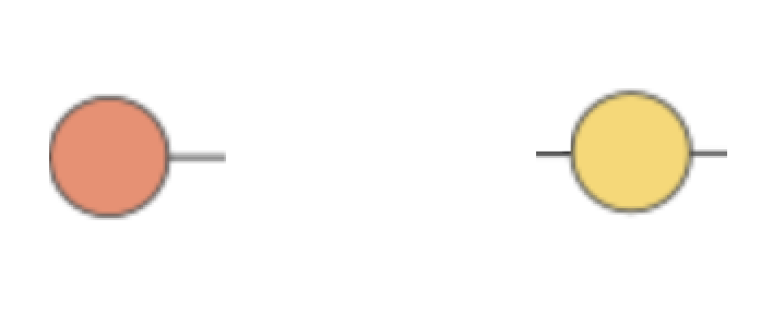
Figure 3. The unit ${\mathbb{I}}=0\in\text{IDAG}^{0}(0)$ of the monoidal structure as a vertex with a single outgoing flag and the unit ${\bf 1}\in\text{IDAG}^{0}(1)$ of the operad structure as a vertex with a single input flag and a single output flag.

It is in fact convenient to describe the unit for the monoidal structure ${\mathbb{I}}=0\in\text{IDAG}^{0}(0)$, given by the single output $0=(\emptyset,\emptyset,\{o\},\emptyset)$, in terms of flags, by viewing the output vertex $\{o\}$ as consisting of a pair $o=(v_{o},f_{o})$ of a vertex $v_{o}$ with an attached outward-oriented flag (half-edge) $f_{o}$, so as to be reminded of the fact that this vertex has a non-empty output set. Note that we have $E=\emptyset$, as there is no pair of flags forming an edge, see Figure 3.

The unit of the operad composition ${\bf 1}\in\text{IDAG}^{0}(1)$, on the other hand consists of a single vertex $v$ together with two half edges $f_{v},f^{\prime}_{v}$, one incoming and one outgoing at $v$, $t(f_{v})=v$ and $s(f^{\prime}_{v})=v$, see Figure 3. The operadic composition $\circ:\text{IDAG}^{0}(k)\times\text{IDAG}^{0}(1)\to\text{IDAG}^{0}(k)$ plugs the outgoing flag of the single output of an object $A$ of $\text{IDAG}^{0}(k)$ into the single input flag $f_{v}$ of ${\bf 1}$, by gluing together the outgoing flag and the ingoing flag $f_{v}$ to an edge $e$, followed by the operation that contracts this edge, so that the vertex $v=t(e)$ is brought to coincide with the vertex $s(e)$ and only the outgoing flas $f^{\prime}_{v}$ remains, while the resulting set of edges (internal edges) of $A\circ{\bf 1}$ agrees with those of $A$ and we have an identification of these two objects. The composition $\circ_{j}:\text{IDAG}^{0}(1)\times\text{IDAG}^{0}(k)\to\text{IDAG}^{0}(k)$ is done similarly with the outgoing flag $f_{v}^{\prime}$ matched with the $j$th incoming flag of $A$ and the resulting edge $e$ then contracted to obtain an identification of ${\bf 1}\circ_{j}A$ and $A$.

2.1.4. Weighted single output IDAGs

We now modify the construction above of the category $\text{IDAG}^{o}$ in order to incorporate data of weights on the edges of the networks. The category $\text{WIDAG}^{o}$ of weighted single-output IDAGs has objects given by pairs $(G,W)$ with $G=(I,H,\{o\},E)$ an IDAG with a single output and $W$ a weight matrix, namely a function $W:V\times V\to{\mathbb{R}}$ where $V=I\sqcup H\sqcup\{o\}$ the set of vertices, with the property that $W(u,v)=0$ whenever $\{e\in E\,|\,s(e)=u,,\,t(e)=v\}=\emptyset$, with $s:E\to I\sqcup H$ and $t:E\to H\sqcup O$ the source and target map. Note that because the graphs in IDAG are assumed to be acyclic, they in particular do not contain looping edges, hence $W(v,v)=0$ for all $v\in V$. Morphisms $\varphi\in{\rm Mor}_{\text{WIDAG}^{o}}((G,W),(G^{\prime},W^{\prime}))$ are morphisms $\varphi:G\to G^{\prime}$ in the category $\tilde{\mathcal{G}}$ of directed graphs described in §2.1.1, with the property that $W^{\prime}=\varphi_{*}(W)$, where the pushforward of the weight matrix is defined as

$$\varphi_{*}(W)(u^{\prime},v^{\prime})=\sum_{\begin{subarray}{c}u\,:\varphi(u)=u^{\prime}\\ v\,:\varphi(v)=v^{\prime}\end{subarray}}W(u,v)\,.$$

If the graph $G$ has parallel edges, namely different edges $e\neq e^{\prime}$ with the same source and target, $s(e)=s(e^{\prime})=v$ and $t(e)=t(e^{\prime})=v^{\prime}$ then the function $W(v,v^{\prime})$ represents a sum of the weights of all the edges connecting $v$ and $v^{\prime}$.

The monoidal structure on $\text{IDAG}^{o}$ defined above induces a monoidal structure on $\text{WIDAG}^{o}$ with

$$(G,W)\oplus(G^{\prime},W^{\prime})=(G\oplus G^{\prime},W\oplus W^{\prime})\,,$$

with $G\oplus G^{\prime}$ defined as above and with $W\oplus W^{\prime}$ given by the following row-column description:

(2.3) $$(W\oplus W^{\prime})((u,o^{\prime}),(v,o^{\prime}))=W(u,v)\ \text{ and }\ (W\oplus W^{\prime})((o,u^{\prime}),(o,v^{\prime}))=W^{\prime}(u^{\prime},v^{\prime})\,.$$

The unit for this monoidal structure is

$$(0,W_{0})=((\emptyset,\emptyset,\{o\},\emptyset),W_{0}(o,o)=0)\,.$$

Note that, for an object $(G,W)\in\text{WIDAG}^{o}$, the condition that there exist a morphism $\varphi:(G,W)\to(0,W_{0})$ amounts to requiring that the map that collapses the whole graph $G$ to the single output vertex $o$ satisfies $\varphi_{*}(W)(o,o)=W_{0}(o,o)=0$, which means

$$\sum_{(u,v)\in V\times V}W(u,v)=0\,.$$

This condition can be seen as an inhibitory-excitatory balance condition over the whole network $G$.

On the other hand, for an object $(G,W)\in\text{WIDAG}^{o}$, the condition that there exist a morphism $\psi:(0,W_{0})\to(G,W)$ implies that the inclusion of the output vertex in $G$ satisfies $\psi_{*}(W_{0})(u,v)=W(u,v)$ for all $(u,v)\in V\times V$. This implies that $W:V\times V\to{\mathbb{R}}$ is the trivial map that is identically zero on all of $V\times V$. Thus, the only objects of $\text{WIDAG}^{o}$ with a morphism from $0$ are those with trivial weights. This shows that the unit $(0,W_{0})$ of the symmetric monoidal structure is neither an initial nor a final object for $\text{WIDAG}^{o}$.

The operad structure on $\text{IDAG}^{o}$ induces an operad structure on $\text{WIDAG}^{o}$, where the composition operations $\circ_{j}$ that match the output vertex $o$ of $(G,W)\in{\mathcal{O}}(n)$ to the $j$-th input vertex $v^{\prime}_{j}$ of $(G^{\prime},W^{\prime})\in{\mathcal{O}}(m)$ give an object $(G\circ_{j}G^{\prime},W\circ_{j}W^{\prime})$, where $G\circ_{j}G^{\prime}$ is the composition in $\text{IDAG}^{o}$ and $W\circ_{j}W^{\prime}$ with entries

(2.4) $$\begin{array}[]{ll}(W\circ_{j}W^{\prime})(u,v)=W(u,v)&\text{when }u,v\in V,\\[8.53581pt] (W\circ_{j}W^{\prime})(u^{\prime},v^{\prime})=W^{\prime}(u^{\prime},v^{\prime})&\text{when }u^{\prime},v^{\prime}\in V^{\prime},\\[8.53581pt] (W\circ_{j}W^{\prime})(u,v^{\prime}_{j})=W(u,o)&\\[8.53581pt] (W\circ_{j}W^{\prime})(o,v^{\prime})=W^{\prime}(v^{\prime}_{j},v^{\prime})&\end{array}$$

and zero otherwise. This composition rule for weights is compatible with the operad axioms. Both (2.3) and (2.4) can be seen as obtained by taking a block sum of the two matrices $W$ and $W^{\prime}$ and then identifying the indices of the vertices that are glued together, merging the corresponding rows and columns.

2.1.5. Category of DNNs

The construction of the category $\text{WIDAG}^{o}$ provides a setting where we can describe computational resources based on DNNs and their compositions where the output of one feeds into input of another, or where two independent ones feed to a single output that integrates their separate inputs. These two types of serial and parallel composition are obtained, respectively, through the operadic composition laws of $\text{WIDAG}^{o}$ and the monoidal structure.

We interpret objects $(G,W)$ of $\text{WIDAG}^{o}$ as feed-forward neural networks, with vertices in $I$ representing the input layer, the unique output $o$ representing the output layer, and the set $H$ of hidden nodes representing the intermediate layers, with $W$ an initialization of weights. Note that we are allowing edges that skip layers. It is known that every directed acyclic graph can be used as architecture for a feed-forward neural network in this way, when connections that skip layers are allowed.

2.2. Threshold dynamics with leak term and the category of DNNs

We first look at the behavior of equation (1.12) (the first case with leak term) when the category of resources is taken to be ${\mathcal{C}}=\text{WIDAG}^{o}$.

The category of network summing functors that we consider for our example of categorical Hopfield dynamics is the category $\Sigma_{\text{WIDAG}^{o}}({\mathfrak{G}})$ for a given network ${\mathfrak{G}}$. As we mentioned in §1 (see [17] for a more detailed account), for a given category of resources ${\mathcal{C}}$ with a properad structure the category $\Sigma_{\mathcal{C}}({\mathfrak{G}})$ of network summing functors (also denoted by $\Sigma_{\mathcal{C}}^{prop}({\mathfrak{G}})$ in [17]) has objects given by functors $\Phi:P(V({\mathfrak{G}}))\to{\mathcal{C}}$, with $P(V({\mathfrak{G}}))$ the category of subsets of $V({\mathfrak{G}})$ with inclusions as morphisms, with the properties:

• summing property: $\Phi({\mathfrak{G}}_{1}\sqcup{\mathfrak{G}}_{2})=\Phi({\mathfrak{G}}_{1})\oplus\Phi({\mathfrak{G}}_{2})$ with $\Phi(\emptyset)=0$;

• connectivity: for all ${\mathfrak{G}}^{\prime}\in P({\mathfrak{G}})$

  $$\Phi({\mathfrak{G}}^{\prime})\in{\rm Obj}({\mathcal{C}}(\deg^{in}({\mathfrak{G}}^{\prime}),\deg^{out}({\mathfrak{G}}^{\prime}))\,,$$

  with $\deg^{in/out}$ the in/out-degree, namely the number of oriented edges entering/leaving the subgraph ${\mathfrak{G}}^{\prime}$ from/to other vertices of $V({\mathfrak{G}})\smallsetminus V({\mathfrak{G}}^{\prime})$.

• compositionality: for all ${\mathfrak{G}}^{\prime},{\mathfrak{G}}^{\prime}\in P({\mathfrak{G}})$,

  (2.5) $$\Phi({\mathfrak{G}}^{\prime}\star{\mathfrak{G}}^{\prime\prime})=\Phi({\mathfrak{G}}^{\prime})\circ_{E({\mathfrak{G}}^{\prime},{\mathfrak{G}}^{\prime\prime})}\Phi({\mathfrak{G}}^{\prime\prime}),$$

  where $E({\mathfrak{G}}^{\prime},{\mathfrak{G}}^{\prime\prime})\subset E({\mathfrak{G}})$ is the set of edges with one endpoint in $V({\mathfrak{G}}^{\prime})$ and the other in $V({\mathfrak{G}}^{\prime\prime})$ and $\circ_{E({\mathfrak{G}}^{\prime},{\mathfrak{G}}^{\prime\prime})}$ is the properad composition that composes outputs to inputs along these edges.

Here we want to consider the case where ${\mathcal{C}}=\text{WIDAG}^{o}$. Since on $\text{WIDAG}^{o}$ we have an operad structure rather than a more general properad, in order to have the correct compositional structure (2.5) for these summing functors, we will assume that the directed graphs ${\mathfrak{G}}$ that we consider here have, at each node, a single output direction and an arbitrary number of inputs.

We think of the network ${\mathfrak{G}}$ as describing the wiring of a population of neurons (labelled by the vertices of ${\mathfrak{G}}$) with their synaptic connections. On the other hand, at each vertex $v$, the object $(G_{v},W_{v})$ describes the DNN that models the neuron labelled by $v$.

Note that here it is important to distinguish between the network ${\mathfrak{G}}$ over which the dynamics takes place, and the networks describing the internal computational architectures assigned to the nodes of ${\mathfrak{G}}$, namely the collection of objects

$$\{(G_{v},W_{v})=\Phi(v)\}_{v\in V(G)}\in{\rm Obj}(\text{WIDAG}^{o})$$

that specify a compositional network summing functor $\Phi\in\Sigma_{\text{WIDAG}^{o}}({\mathfrak{G}})$. We use the notation ${\mathfrak{G}}$ for the underlying network (rather than $G$ as in §1 above) to avoid any possible confusion.

We only assume here that the graph ${\mathfrak{G}}$ is a finite directed graph. We do not require that it is acyclic. In general we allow for the possibility that ${\mathfrak{G}}$ has multiple edges and looping edges. We also do not require any particular structure of inputs and outputs for ${\mathfrak{G}}$. On the other hand the graphs $G_{v}$ are in the category $\text{IDAG}^{o}$ hence we assume they are acyclic, with a single output vertex, and with single outgoing edges at other vertices, and with a single incoming flag at input vertices and a single outgoing flag at the output vertex.

We can then write the categorical Hopfield equations in the category of compositional summing functors $\Sigma_{\text{WIDAG}^{o}}({\mathfrak{G}})$ as

(2.6) $$(G_{v}(n+1),W_{v}(n+1))=(G_{v}(n),W_{v}(n))\oplus\left(\oplus_{v^{\prime}\in V({\mathfrak{G}})}T_{vv^{\prime}}(G_{v^{\prime}}(n),W_{v^{\prime}}(n))\oplus(\tilde{G}_{v},\tilde{W}_{v})\right)_{+}\,.$$

Thus, here the next step of the dynamics takes the graph with weights $(G_{v}(n),W_{v}(n))$ of the current step and glues it at the output with another graph, which is either the trivial single output graph when the last term is below threshold and is a sum of the graphs with weights $(G_{v^{\prime}}(n),W_{v^{\prime}}(n))$, transformed via the functors $T_{vv^{\prime}}$ and the assigned (bias term) graph with weights $(\tilde{G}_{v},\tilde{W}_{v})$, when this sum term is above threshold. This is illustrated in Figure 4.

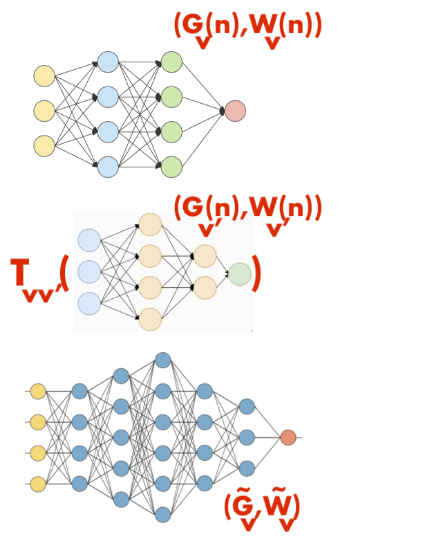
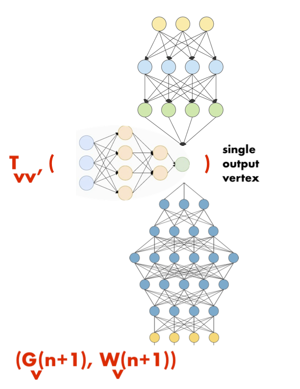
Figure 4. The update rule (2.6) of the dynamics takes the objects $(G_{v}(n),W_{v}(n))$ and $(\tilde{G}_{v},\tilde{W}_{v})$ at the vertex $v$ and the $T_{vv^{\prime}}(G_{v^{\prime}}(n),W_{v^{\prime}}(n))$ and glues their outputs together to a single output to obtain the updated $(G_{v}(n+1),W_{v}(n+1))$.

Here $(\tilde{G}_{v},\tilde{W}_{v})$ is an assigned summing functor which plays the role of a “bias term” at each node $v\in V({\mathfrak{G}})$. This can be taken to be $(0,W_{0})$ at all $v$, for example. A possible choice of the collection $T=\{T_{vv^{\prime}}\}_{v,v^{\prime}\in V({\mathfrak{G}})}$ of endofunctors of $\text{WIDAG}^{o}$ will be discussed in §2.3.2 below. The threshold $(\cdot)_{+}$ imposes an inhibitory-excitatory balance condition on the resulting DNNs

(2.7) $$({\mathbb{G}}_{v},{\mathbb{W}}_{v})(n):=\oplus_{v^{\prime}\in V({\mathfrak{G}})}T_{vv^{\prime}}(G_{v^{\prime}}(n),W_{v^{\prime}}(n))\oplus(\tilde{G}_{v},\tilde{W}_{v}).$$

Indeed the threshold detects whether there are non-trivial morphisms,

$${\rm Mor}_{\text{WIDAG}^{o}}(({\mathbb{G}}_{v},{\mathbb{W}}_{v})(n),(0,W_{0}))\neq\emptyset.$$

As discussed above this condition is satisfied provided that ${\mathbb{W}}_{v}$ satisfies the inhibitory-excitatory balance condition

$$\sum_{a,b\in V({\mathbb{G}}_{v})}{\mathbb{W}}_{v}(a,b)=0.$$

When the balance condition above fails, the threshold replaces $({\mathbb{G}}_{v},{\mathbb{W}}_{v})(n)$ with the unit $(0,W_{0})$ so that the equation stabilizes, with

$$(G_{v}(n+1),W_{v}(n+1))=(G_{v}(n),W_{v}(n)).$$

Thus, the dynamics reaches a fixed point at the first $n\in{\mathbb{N}}$ for which the balance condition of $({\mathbb{G}}_{v},{\mathbb{W}}_{v})(n)$ is violated.

If the balance condition is not violated at any $n\in{\mathbb{N}}$, then a solution is given by a non-stationary sequence $(G_{v}(n),W_{v}(n))$. This can be seen as a sequence $\Phi_{n}$ of compositional network summing functors in $\Sigma_{\text{WIDAG}^{o}}({\mathfrak{G}})$. One can ask if and in what sense this solution may approach a fixed point.

As discussed in [17], the evolution $\Phi_{n}\mapsto\Phi_{n+1}$ is implemented by an endofunctor ${\mathcal{T}}$ of the category $\Sigma_{\text{WIDAG}^{o}}({\mathfrak{G}})$ that maps ${\mathcal{T}}:\Phi\mapsto(T(\Phi)\oplus\tilde{\Phi})_{+}$ where $\tilde{\Phi}$ is the summing functor defined by the local data $(\tilde{G}_{v},\tilde{W}_{v})$, $T$ is the endofunctor implemented on the local data by the $T_{vv^{\prime}}$, and the threshold is seen as in [17] as an endofunctor (not necessarily monoidal) of $\hat{\mathcal{C}}$. Thus, stationary solutions can be viewed as fixed points of the endofunctor ${\mathcal{T}}$. As we discussed in §1.3.1 above, according to the general notion of fixed points of endofunctors, this means here that stationary solutions are summing functors $\Phi\in\Sigma_{\text{WIDAG}^{o}}({\mathfrak{G}})$ that are isomorphic to their image under this endofunctor, $\Phi\simeq{\mathcal{T}}(\Phi)$. This condition corresponds to the existence of isomorphisms in ${\mathcal{C}}$

$$\eta_{v}:(G_{v},W_{v})\stackrel{{\scriptstyle\simeq}}{{\rightarrow}}(G_{v},W_{v})\oplus\left(\bigoplus_{v^{\prime}}T_{vv^{\prime}}(G_{v^{\prime}},W_{v^{\prime}})\oplus(\tilde{G}_{v},\tilde{W}_{v})\right)_{+}\,,$$

where $\Phi_{v}=(G_{v},W_{v})$.

Even though we have not specified so far a choice of the endofunctors $T_{vv^{\prime}}$ of ${\mathcal{C}}$, we can already make some general comments about the behavior of solutions in this specific example of categorical Hopfield dynamics. Indeed, the fixed point condition above, in the case where the balance condition holds on the right-hand-side, so that the threshold is the identity, in particular implies that the underlying directed graphs are related by an isomorphism

$$\eta_{v}:G_{v}\stackrel{{\scriptstyle\simeq}}{{\rightarrow}}G_{v}\oplus{\mathbb{G}}_{v}$$

with $({\mathbb{G}}_{v},{\mathbb{W}}_{v})$ as above. By our definition of the monoidal structure in $\text{WIDAG}^{o}$, the graph $G_{v}\oplus{\mathbb{G}}_{v}$ has vertex set $V(G_{v}\oplus{\mathbb{G}}_{v})=V(G_{v})\times\{o^{\prime}\}\sqcup\{o\}\times V({\mathbb{G}}_{v})$, where $o$ is the single output vertex of $G_{v}$ and $o^{\prime}$ is the single output vertex of ${\mathbb{G}}_{v}$. The existence of an isomorphism between $G_{v}$ and $G_{v}\oplus{\mathbb{G}}_{v}$ would require $V(G_{v})\simeq V(G_{v}\oplus{\mathbb{G}}_{v})$, which can happen only if ${\mathbb{G}}_{V}=\{o^{\prime}\}$ so that necessarily $({\mathbb{G}}_{v},{\mathbb{W}}_{v})=(0,W_{0})$. Thus, we see that in this case the only fixed points are indeed those $(G_{v},W_{v})$ such that $({\mathbb{G}}_{v},{\mathbb{W}}_{v})=(0,W_{0})$. Note that, because $({\mathbb{G}}_{v},{\mathbb{W}}_{v})$ is a monoidal sum

$$({\mathbb{G}}_{v},{\mathbb{W}}_{v})=\bigoplus_{v^{\prime}}T_{vv^{\prime}}(G_{v^{\prime}},W_{v^{\prime}})\oplus(\tilde{G}_{v},\tilde{W}_{v})\,,$$

in order to have $({\mathbb{G}}_{v},{\mathbb{W}}_{v})=(0,W_{0})$ we would need each term in the sum to be $T_{vv^{\prime}}(G_{v^{\prime}},W_{v^{\prime}})=(0,W_{0})$ and $(\tilde{G}_{v},\tilde{W}_{v})$. However, we know this is not the case, either because the bias term $(\tilde{G}_{v},\tilde{W}_{v})$ is taken to be nontrivial, or because at least some of the $T_{vv^{\prime}}(G_{v^{\prime}},W_{v^{\prime}})$ are nontrivial. We then reach the conclusion that $({\mathbb{G}}_{v},{\mathbb{W}}_{v})=(0,W_{0})$ cannot be satisfied if $({\mathbb{G}}_{v},{\mathbb{W}}_{v})$ satisfies the balanced condition and no fixed points can occur in this case, since we cannot then have an isomorphism between $(G_{v},W_{v})$ and $(G_{v},W_{v})\oplus({\mathbb{G}}_{v},{\mathbb{W}}_{v})$. Thus, fixed points only occur when $({\mathbb{G}}_{v},{\mathbb{W}}_{v})$ violates the balanced condition.

We can also consider the notion of strict fixed point recalled in §1.3.1. The summing functors $\Phi_{n}$ determined by the objects $\{(G_{v}(n),W_{v}(n))\}$ in turn determine a sequence of vertices in the simplicial set given by the nerve ${\mathcal{N}}(\Sigma_{\mathcal{C}}({\mathfrak{G}}))$. The endofunctor ${\mathcal{T}}$ induces a map of simplicial sets ${\mathcal{T}}_{\mathcal{N}}:{\mathcal{N}}(\Sigma_{\mathcal{C}}({\mathfrak{G}}))\to{\mathcal{N}}(\Sigma_{\mathcal{C}}({\mathfrak{G}}))$. A fixed point $x={\mathcal{T}}_{\mathcal{N}}(x)$ in ${\mathcal{N}}(\Sigma_{\mathcal{C}}({\mathfrak{G}}))$ corresponds to a strict fixed point for the endofunctor ${\mathcal{T}}$, namely an object $\Phi\in\Sigma_{\mathcal{C}}({\mathfrak{G}})$ such that $\Phi={\mathcal{T}}(\Phi)$ (actually equal rather than just isomorphic, see [16]).

On the other hand, since morphisms in the category $\Sigma_{\mathcal{C}}({\mathfrak{G}})$ are just invertible natural transformations, a vertex $x$ of ${\mathcal{N}}(\Sigma_{\mathcal{C}}({\mathfrak{G}}))$ such that $x$ and ${\mathcal{T}}_{\mathcal{N}}(x)$ are connected by an edge of ${\mathcal{N}}(\Sigma_{\mathcal{C}}({\mathfrak{G}}))$ correspond to a fixed point in the more general sense considered above. Thus, we can take as a possible definition of an orbit $\{\Phi_{n}\}_{n\in{\mathbb{N}}}$, with $\Phi_{n+1}={\mathcal{T}}(\Phi_{n})$, converging to a fixed point, the requirement that the induced sequence of vertices $x_{n}$ in ${\mathcal{N}}(\Sigma_{\mathcal{C}}({\mathfrak{G}}))$ approaches either a single vertex or a sequence of vertices successively connected by an edge. Here we can use the topology of the realization $|{\mathcal{N}}(\Sigma_{\mathcal{C}}({\mathfrak{G}}))|$ to measure proximity.

Observe then that, for the same reason discussed above, if we have a non-stationary sequence $(G_{v}(n),W_{v}(n))$, where the balanced condition is satisfied at all $n$, we necessarily have, at each step

$$\#V(G_{v}(n+1))>\#V(G_{v}(n))\,,$$

so the sequence $\#V(G_{v}(n))$ is divergent at every $v\in V({\mathfrak{G}})$ where the balanced condition holds for all $n$. This exclude the possibility that the corresponding sequence of vertices in ${\mathcal{N}}(\Sigma_{\mathcal{C}}({\mathfrak{G}}))$ would stabilize to either $x_{n}={\mathcal{T}}_{\mathcal{N}}(x_{n})$ or to $x_{n}$ and ${\mathcal{T}}_{\mathcal{N}}(x_{n})$ connected by an edge (an isomorphism in $\Sigma_{\mathcal{C}}({\mathfrak{G}})$) as both conditions would require the number of vertices of $G_{v}(n)$ to stabilize.

Thus, regardless of the specific choice of the family of endomorphisms $T_{vv^{\prime}}$, we see that in the case of the first equation (1.12), solutions converge to a fixed point (in finitely many steps) if and only if the balanced condition on $({\mathbb{G}}_{v},{\mathbb{W}}_{v})$ is violated after finitely many steps and the other solutions do not converge to fixed points.

Assuming that $(G_{v}(n),W_{v}(n))$ satisfies the balanced condition, the violation of the balanced condition for $({\mathbb{G}}_{v},{\mathbb{W}}_{v})$ depends on the choice of $T_{vv^{\prime}}$ and of $(\tilde{G}_{v},\tilde{W}_{v})$. Since these are chosen with the equation, we can just assume for simplicity that the objects $(\tilde{G}_{v},\tilde{W}_{v})$ do satisfy the balanced condition, so that the possible violations are only coming from the choice of the endofunctors $T_{vv^{\prime}}$ and not from the combined effect of the two choices. Thus, the question of the violation of the balanced condition becomes a question of when the object $\oplus_{v^{\prime}\in V({\mathfrak{G}})}T_{vv^{\prime}}(G_{v^{\prime}},W_{v^{\prime}})$ fails to satisfy the balanced condition.

2.3. Threshold dynamics without leak term and the category of DNNs

We now consider the second case (without leak term) of the categorical Hopfield dynamics given by equation (1.13) with ${\mathcal{C}}=\text{WIDAG}^{o}$. We are assuming the same hypothesis about the underlying network ${\mathfrak{G}}$ and about the graphs $G_{v}$ as in §2.2.

In this setting without leak term, instead of (2.6) the equation we consider is of the form

(2.8) $$(G_{v}(n+1),W_{v}(n+1))=\left(\oplus_{v^{\prime}\in V({\mathfrak{G}})}T_{vv^{\prime}}(G_{v^{\prime}}(n),W_{v^{\prime}}(n))\oplus(\tilde{G}_{v},\tilde{W}_{v})\right)_{+}\,.$$

Stationary solutions occur in two cases:

1. for pairs $(G_{v},W_{v})$ where the right-hand-side $\oplus_{v^{\prime}\in V({\mathfrak{G}})}T_{vv^{\prime}}(G_{v^{\prime}},W_{v^{\prime}})\oplus(\tilde{G}_{v},\tilde{W}_{v})$ satisfies the balanced condition and

   (2.9) $$(G_{v},W_{v})=\oplus_{v^{\prime}\in V({\mathfrak{G}})}T_{vv^{\prime}}(G_{v^{\prime}},W_{v^{\prime}})\oplus(\tilde{G}_{v},\tilde{W}_{v}),$$

2. in cases where the right-hand-side does not satisfy the balanced condition and the datum $(\tilde{G}_{v},\tilde{W}_{v})$ also does not satisfy the balanced condition.

In the second case the stationary solution is the unit $(0,W_{0})$ of the monoidal structure. We focus on some particular examples of the first case, where depending on the choice of the endofunctors $T_{vv^{\prime}}$ and the datum $(\tilde{G}_{v},\tilde{W}_{v})$ we find different behaviors of stationary solutions. In particular, in §2.3.1 we analyze a very simplified toy model case.

We use the same notation $({\mathbb{G}}_{v},{\mathbb{W}}_{v})$ as in (2.7). In the first case, the fixed point condition (2.9) in particular implies that $G_{v}\simeq{\mathbb{G}}_{v}$ are isomorphic as directed graphs.

2.3.1. Decoupled dynamics

In order to give a very basic example of the dynamics (2.8), we make a drastic simplifying assumption on the form of the endofunctors $T_{vv^{\prime}}$ that completely decouples the dynamics at the individual nodes $v\in V({\mathfrak{G}})$ from the structure of the graph ${\mathfrak{G}}$. This is, of course, a very non-realistic assumption, as in general one wants the $T_{vv^{\prime}}$ to reflect the connectivity structure of ${\mathfrak{G}}$, but it is useful for the purpose of presenting a simple explicit example. In particular, this simplified setting of uncoupled dynamics will suffice to show (see §2.3.2 below) that backpropagation in DNNs arises as a special case of our categorical Hopfield dynamics.

Let us then consider the case where the endofunctors $T_{vv^{\prime}}$ have the form $T_{vv^{\prime}}=T_{v}\delta_{v,v^{\prime}}$ where here the Kronecker delta $\delta_{v,v^{\prime}}$ means that for $v\neq v^{\prime}$ the endofunctor $T_{vv^{\prime}}$ maps all objects to the unit $(0,W_{0})$. The endofunctors $T_{v}$ are taken to be unital monoidal endofunctors of ${\mathcal{C}}$. In particular they map $(0,W_{0})$ to itself. (If we want to think of the $T_{vv^{\prime}}$ in terms of graph edges, this would correspond to a network ${\mathfrak{G}}$ that has a looping edge at each vertex, and this edge is solely responsible for the dynamics.)

We also assume that the endofunctors $T_{v}$ of ${\mathcal{C}}$ act on objects $(G_{v},W_{v})$ by maintaining the same underlying graph and updating the weights,

(2.10) $$T_{v}(G_{v},W_{v})=(G_{v},T_{v}(W_{v}))\,.$$

Under these simplifying assumptions, we see by the same argument used in the case of equation (2.6) that the isomorphism of directed graphs $G_{v}\simeq{\mathbb{G}}_{v}=G_{v}\oplus\tilde{G}_{v}$ is possible only if the term $(\tilde{G}_{v},\tilde{W}_{v})=(0,W_{0})$. We then have the fixed point condition of the form

(2.11) $$(G_{v},W_{v})=(G_{v},T_{v}(W_{v}))\,,$$

where (as discussed in §1) we interpret the “$=$” sign in the equations as isomorphism rather than equality, so that we consider also non-strict fixed points (see §1.3.1). An isomorphism $\varphi:(G_{v},W_{v})\to(G_{v},T_{v}(W_{v}))$ is an automorphism $\varphi:G_{v}\to G_{v}$, namely bijections $\varphi_{V}:V(G_{v})\to V(G_{v})$ and $\varphi_{E}:E(G_{v})\to E(G_{v})$ compatible with source, target, and $\epsilon$ morphisms (see §2.1.1) and such that for all vertices $a,b\in V(G_{v})$

$$T_{v}(W_{v})(\varphi(a),\varphi(b))=W_{v}(a,b)\,.$$

In particular, in §2.3.2 we focus on the case of strict fixed points where $\varphi$ is the identity and $T_{v}(W_{v})=W_{v}$. This is a fixed point condition for the updating of the weights $W_{v}$ through the map $T_{v}$.

Thus, the kind of dynamics we are considering here consists of performing an update on the weights of the individual DNN machines $(G_{v},W_{v})$ located at each node $v$ of the network ${\mathfrak{G}}$, where the update of the weights is performed by the functor $T_{v}$. For DDNs a typical example of update of the weights is the backpropagation mechanism, realized via a gradient descent algorithm. We will show in §2.3.2 that indeed backpropagation fits in the functorial formulation we are presenting here.

Of course this case is oversimplistic as it assumes that the updating of the weights of each machine $(G_{v},W_{v})$ is independent of the inputs/outputs it received/transmits to the machines placed at other nodes of ${\mathfrak{G}}$. However, it is useful to consider as a simplest example.

2.3.2. Functorial gradient descent

Let us consider a simple mechanism for updating the weights $W_{v}$ of the DNN $(G_{v},W_{v})$ in terms of gradient descent with respect to a given cost function. We write $F_{v}$ for the given relevant cost function, which we assume is specific to the DNN $(G_{v},W_{v})$ and therefore varies with the choice of $v\in V({\mathfrak{G}})$. We also fix a scale $\epsilon>0$, the learning rate. This can be taken uniform over $V({\mathfrak{G}})$, since this set is finite. Then the updating of the weights by gradient descent take on the usual form

(2.12) $$T_{v}(W_{v}):=W_{v}-\epsilon\nabla_{W_{v}}F_{v}\,,$$

so that the condition that $W_{v}$ is a fixed point, $T(W_{v})=W_{v}$, corresponds to the condition that the weights $W_{v}$ are a critical point of the cost function, which under additional conditions on the shape of the cost function can be assumed to be a minimum.

In our setting, we need to ensure that (2.12) indeed defines an endofunctor of $\text{WIDAG}^{o}$. Given a cost function $F$ we map an object $(G,W)$ of $\text{WIDAG}^{o}$ to

$$T(G,W)=(G,W-\epsilon\nabla_{W}F)\,.$$

Given a morphism $\varphi\in{\rm Mor}_{\text{WIDAG}^{o}}((G,W),(G^{\prime},W^{\prime}))$, with $\varphi:G\to G^{\prime}$ a morphism of directed graphs and $W^{\prime}=\varphi_{*}(W)$, we define $T(\varphi)$ as the same morphism $\varphi:G\to G^{\prime}$, since $T$ does not change the underlying graph. Thus, for this to give a morphism $T(\varphi)\in{\rm Mor}_{\text{WIDAG}^{o}}((G,T(W)),(G^{\prime},T(W^{\prime})))$ we just need to check the consistency

$$T(W^{\prime})=\varphi_{*}\,T(W)\,.$$

The right-hand-side is given by

$$(\varphi_{*}\,T(W))(u^{\prime},v^{\prime})=\sum_{\begin{subarray}{c}u\,:\varphi(u)=u^{\prime}\\ v\,:\varphi(v)=v^{\prime}\end{subarray}}T(W)(u,v)=\sum_{u,v}W(u,v)-\epsilon\sum_{u,v}\nabla_{W(u,v)}F$$

which agrees with $W^{\prime}(u^{\prime},v^{\prime})-\epsilon\nabla_{W^{\prime}(u^{\prime},v^{\prime})}F=T(W^{\prime})(u^{\prime},v^{\prime})$.

Thus, with this particular choice of the endofunctors $T_{vv^{\prime}}=T_{v}\delta_{v,v^{\prime}}$, the stationary solutions of the equation (2.8) are given by $\{(G_{v},W_{v})\}$ where the graphs $G_{v}$ are as in the chosen initial datum of the equation, $G_{v}(n)=G_{v}(0)$, for all $n\in{\mathbb{N}}$, and where the weights $W_{v}$ are minima of assigned cost functions $F_{v}$ (we think of the cost functions as being part of the data specifying the functor $T_{v}$). In this case we have a notion of convergence of a solution to a fixed point, by the requirement that the sequence of weights $W_{v}(n)$ converge to a minimum of $F_{v}$.

Note that the type of functoriality we are considering here is different from the functorial backpropagation discussed in [8]. The latter is more closely related to our operadic compositional structure than to the functoriality with respect to the category ${\mathcal{C}}=\text{WIDAG}^{o}$ discussed here.

Acknowledgment

The author is partially supported by NSF grants DMS-1707882 and DMS-2104330 and by FQXi grants FQXi-RFP-1 804 and FQXi-RFP-CPW-2014, SVCF grant 2020-224047.

References

- [1] D.J. Amit, Modeling Brain Function. The World of Attractor Neural Networks, Cambridge University Press, 1989.
- [2] D. Beniaguev, I. Segev, M. London, Single cortical neurons as deep artificial neural networks, Neuron 109 (2021) 2727–2739.
- [3] R. Brown, I. Morris, J. Shrimpton, C.D. Wensley, Graphs of morphisms of graphs, The Electronic Journal of Combinatorics, Vol. 15 (2008) Paper A1 [28 pages].
- [4] N. Brunel, Dynamics of Sparsely Connected Networks of Excitatory and Inhibitory Spiking Neurons, Journal of Computational Neuroscience 8 (2000), 183–208.
- [5] S. Chowdhury, T. Gebhart, S. Huntsman, M. Yutin, Path homologies of deep feedforward networks, arXiv:1910.07617
- [6] B. Coecke, T. Fritz, R.W. Spekkens, A mathematical theory of resources, Information and Computation 250 (2016), 59–86. [arXiv:1409.5531]
- [7] M. Fiore, M. Devesas Campos, The algebra of directed acyclic graphs, in “Computation, logic, games, and quantum foundations”, pp. 37–51, Lecture Notes in Comput. Sci., 7860, Springer, 2013.
- [8] B. Fong, D. Spivak, R. Tuyéras, Backprop as functor: a compositional perspective on supervised learning, in “34th Annual ACM/IEEE Symposium on Logic in Computer Science (LICS)”, IEEE, 2019 [13 pages]
- [9] T. Fritz, Resource convertibility and ordered commutative monoids, Math. Str. Comp. Sci. 27 (2017) N. 6, 850–938 [arXiv:1504.03661]
- [10] A. Ganchev, Control and composability in deep learning – Brief overview by a learner, in “Lie Theory and its Applications in Physics”, pp. 519–526, Springer, 2020.
- [11] W. Gerstner, W.M. Kistler, R. Naud, L. Paninski, Neuronal Dynamics, Cambridge University Press, 2014.
- [12] J.J. Hopfield, Neural networks and physical systems with emergent collective computational abilities, Proc. Natl. Acad. Sci. USA, Vol. 79 (1982) 2554–2558.
- [13] J.J. Hopfield, Neurons with graded response have collective computational properties like those of two-state neurons. Proc. Nat. Acad. Sci. USA, Vol. 81 (1984) 3088–3092.
- [14] J. Kock, Graphs, hypergraphs, and properads, arXiv:1407.3744
- [15] J. Lambek. A fixpoint theorem for complete categories, Math. Z. 103 (1968), 151–161.
- [16] A. Luzhenkov, A note on fixed points of endofunctors, arXiv:1704.04414v2
- [17] Yu.I. Manin, M. Marcolli, Homotopy Theoretic and Categorical Models of Neural Information Networks, arXiv:2006.15136.
- [18] M. Marcolli, Topological Models of Neural Information Networks, in “Geometric Science of Information. 5th International Conference, GSI 2021”, Lecture Notes in Computer Science, Vol. 12829, pp. 623–633, Springer, 2021.
- [19] M. Marcolli, D. Tsao, Toward a topological model of consciousness and agency, white paper for the FQXi Foundation, 2018.
- [20] M. Markl, Operads and PROPs, in “Handbook of algebra”. Vol. 5, pp. 87–140, Elsevier and North-Holland, 2008.
- [21] R.W. Thomason, First quadrant spectral sequences in algebraic -theory via homotopy colimits, Comm. Algebra 10 (1982), no. 15, 1589–1668.
- [22] R.W. Thomason, Symmetric monoidal categories model all connective spectra, Theory Appl. Categ. 1 (5) (1995) 78–118.
- [23] G. Segal, Categories and cohomology theories, Topology 13 (1974) 293–312.
- [24] B. Valette, A Koszul duality for PROPs, Trans. Amer. Math. Soc. 359 (2007), 4865–4943.
- [25] C. van Vreeswijk, H. Sompolinsky, Chaotic Balanced State in a Model of Cortical Circuits, Neural Computation 10 (1998), 1321–1371.
- [26] G. Winskel, M. Nielsen, Categories in concurrency, in “Semantics and logics of computation (Cambridge, 1995)”, pp. 299–354, Publ. Newton Inst., 14, Cambridge Univ. Press, 1997.
- [27] S. Zhou, Y. Yu, Synaptic E–I Balance Underlies Efficient Neural Coding, Frontiers in Neuroscience, Vol.12 (2018) Article 46 [11 pages]