Microscopic Theory of Nuclear Fission

Abstract

Nuclear fission represents the ultimate test for microscopic theories of nuclear structure and reactions. Fission is a large-amplitude, time-dependent phenomenon taking place in a self-bound, strongly-interacting many-body system. It should, at least in principle, emerge from the complex interactions of nucleons within the nucleus. The goal of microscopic theories is to build a consistent and predictive theory of nuclear fission by using as only ingredients protons and neutrons, nuclear forces and quantum many-body methods. Thanks to a constant increase in computing power, such a goal has never seemed more within reach. This chapter gives an overview both of the set of techniques used in microscopic theory to describe the fission process and of some recent successes achieved by this class of methods.

1 Introduction

Atomic nuclei can sometimes, either spontaneously or after bombardment by external particles, split into two or more fragments. This fission process was discovered experimentally in late 1938 by Hahn and Strassman Hahn and Strassmann (1938, 1939). Barely six months later, Bohr and Wheeler, building on a critical insight by Lise Meitner Meitner and Frisch (1939), proposed the first model of the process Bohr and Wheeler (1939). Since then considerable effort has been expended to understand this phenomenon. In the past few years, there has been a renaissance in fission studies and, as a result, several review articles and textbooks have been published on this subject Krappe and Pomorski (2012); Schunck and Robledo (2016); Andreyev et al. (2017); Schmidt and Jurado (2018); Younes et al. (2019); Younes and Loveland (2021). This chapter will focus on the most recent developments in building a microscopic theory of fission. Therefore, the interested reader is advised to consult the aforementioned references to gain a more complete picture of this fascinating problem.

1.1 Fission Observables

The complexity of the fission process translates into a large number of observables, that is, quantities that can be measured experimentally and, in principle, computed theoretically. One may classify these observables into three main categories.

The first category corresponds to the probability that fission takes place in a nucleus given a set of initial conditions. The case of spontaneous fission is the simplest one: the initial conditions are nothing but the number of protons and neutrons of the nucleus, which is assumed to be in its ground state, and the probability of fission is encoded in the spontaneous fission half life $\tau_{\rm SF}$. The case of induced fission is much more involved. First, the initial conditions now include the full characteristics of the incident particle such as its identity (neutron, photon, proton, $\alpha$ particle, etc.), its energy and possibly its quantum numbers, but also the characteristics of the target nucleus which may or may not be in its ground state. The collision of the incident particle with the target nucleus may take many different forms: elastic scattering (the neutron is simply deflected without transfer of energy), inelastic scattering (deflection with transfer of energy to the target), or capture. Even if the neutron is captured, there is no guarantee that the resulting excited nucleus will fission. It may decay by emitting one or several neutrons (noted as the $(n,xn)$ channel); it may emit a series of photons, the $(n,\gamma)$ channel; it may beta decay, the $(n,\beta)$ channel; or it may fission, the $(n,f)$ channel. This list is not exhaustive and many other channels are potentially available. How the competition between these different channels affects the probability of fission is encoded in what called the fission cross section. Both the spontaneous fission half life and the fission cross section can be measured, at least in some nuclei, with high precision.

The second category of observables corresponds, roughly speaking, to the outcome of the deformation process that leads the nucleus to its breaking point, or scission point. At scission, the initial fission fragments have been formed. Each fragment is characterized by its number of protons $Z$ and number of neutrons $N$, its excitation energy $E^{*}$, its spin distribution $p(J)$ and its level density $\rho(E)$. When a sample of material is irradiated every fission event that occurs is different: there is a probability that a fragment $(Z,N)$ is formed and this probability is encoded in what is called the primary fission fragment distribution. It is customary to use the notation $Y(Z,A)$ to refer to the probability (normalized to 200) that a fragment with charge $Z$ and total mass $A$ is formed. Marginal distributions $Y(Z)$ (the charge distribution) and $Y(A)$ (the mass distribution) can be obtained by integrating $Y(Z,A)$ over $A$ and $Z$, respectively. It is essential to realize that all the aforementioned quantities cannot be measured because of the extremely short time scale at which fission takes place, of the order of $\tau_{f}\approx 10^{-19}$ s: they must be computed by theoretical models. These models must be predictive since the results of the calculations cannot be directly compared with data. In fact, the predictions of $Y(Z,A)$, $E^{*}$, $p(J)$, etc., will serve as inputs to the statistical reaction theory codes that model the deexcitation of the fragments.

This deexcitation phase yields a third class of fission observables, which include the characteristics of all the particles that can be emitted. The first, prompt emission phase involves mostly neutrons and photons ($\gamma$ rays). Observables associated with these particles include the mean number of neutrons emitted, $\bar{\nu}$, the average energy of the neutron, the mean number of $\gamma$ emitted (called the photon or $\gamma$ multiplicity), $N_{\gamma}$, the angular correlations between the neutrons, the photons, or the neutrons and the photons, etc. After the prompt emission phase, a number of $\beta$ decays may take place. They will result in the emission of electrons and antineutrinos.

1.2 Physics Concepts

The ultimate goal of any microscopic approach to fission is to achieve a description of this process based only on our knowledge of in-medium nuclear forces and quantum many-body methods. In an ideal world, this description would be based on solving the following equation

$$\ket{\Psi}_{\rm f}=e^{-\frac{it}{\hbar}\hat{H}}\ket{\Psi}_{\rm i},$$ (1)

where $\ket{\Psi}_{\rm i}$ and $\ket{\Psi}_{\rm i}$ are, respectively, the initial state of the nucleus before fission and the final state after the process has completed, and $\hat{H}$ is the nuclear many-body Hamiltonian. This naive approach is faced with formidable challenges:

• The nuclear many-body Hamiltonian $\hat{H}$ is not known exactly. Our best current model of it is based on chiral effective field theory Weinberg (1990); Machleidt and Sammarruca (2016); Hammer et al. (2020). The characteristic features of $\hat{H}$, most notably the short range of nuclear fores and the presence of 3-, 4- and generally $N$-body interaction terms, make determining the nuclear wave functions an extremely challenging problem even in the lightest nuclei Barrett et al. (2013). In recent years, the scope of ab initio methods – very loosely defined here as the set of methods trying to solve the nuclear many-body problem with a microscopic Hamiltonian $\hat{H}$ such as the one from chiral EFT – has extended tremendously thanks to the introduction of powerful many-body techniques and the constant improvement of supercomputers Hagen et al. (2014); Carlson et al. (2015); Hergert et al. (2016); Stroberg et al. (2019). Unfortunately, these methods cannot reach the region of actinides and superheavy nuclei where fission is relevant and remain largely focused on static properties of nuclei. Furthermore, the precision of such calculations is not sufficient yet.

• The very definition of the initial and final states in (1) is far from trivial. In all types of fission, the final state involves not a single nucleus, but a pair of fragments together with a number of emitted particles (neutrons, photons, possibly electrons and anti-neutrinos if $\beta$-decay is included). Even the determination of the initial wave function $\ket{\Psi}_{\rm i}$ is a challenge. In spontaneous fission, it is associated with the ground state of the nucleus and might thus, in a near future, be within reach of ab initio methods. In the case of induced, fission, however, it entails characterizing the absorption of an incoming particle (neutron or photon, typically) by a heavy target nucleus for a broad range of incident energies. Extending the methods used in light-ion reactions Baroni et al. (2013) to such heavy nuclei is not an easy task.

For these reasons, the adjective “microscopic” in this chapter will take a rather narrow definition. It will refer to the set of methods globally known as energy density functional theory (EDF) Schunck (2019). Most of the techniques developed in the EDF approach are about finding good approximations to the nuclear many-body wave function without having to deal with determining the spectrum of the true nuclear many-body Hamiltonian $\hat{H}$. By construction, the EDF theory thus contains a higher degree of phenomenology than ab initio approaches. At the same time, it is still a many-body theory of the nucleus, by contrast with, e.g., the liquid drop model.

Ever since the very first model of the process by Bohr and Wheeler Bohr and Wheeler (1939), fission has always been thought of as an extreme deformation process. This concept is very easily built in phenomenological approaches based on the liquid drop model. However, since the nuclear Hamiltonian $\hat{H}$ is invariant under rotations, the nuclear wave functions $\ket{\Psi}$ should also be rotationally invariant and characterized by good angular momentum. Clearly, this is not compatible with the concept of deformation. This could pose interesting conceptual difficulties if fission were described with ab initio methods; in the context of the EDF approach, deformation is in fact a natural consequence of a phenomenon called spontaneous symmetry breaking Duguet (2014); Schunck (2019). When solving the Hartree-Fock or Hartree-Fock-Bogoliubov equation of the single-reference EDF theory (see below), solutions that break some or all of the symmetries of the nuclear Hamiltonian can lower the energy of the system. This effect, also known as the Jahn-Teller effect, is present in many fields of physics, from nuclei to electronic systems to quantum field theory; see Nazarewicz (1994) for a discussion in the context of nuclear physics.

The concept of spontaneous symmetry breaking is also closely related to the one of collective variables. In molecular systems, for example, the separation of all degrees of freedom into slow, collective ones associated with the coordinates $R_{i}$ of the ions and the fast, intrinsic degrees of freedom related to the electrons is straightforward. In nuclear systems, this distinction is less clear but still applies. As recognized a long time ago, the low-lying spectrum of nuclei contains sequences of excited states that suggest strong collective behavior of the nucleus as whole, akin to collective vibrations and rotations Bohr and Mottelson (1998); Ring and Schuck (2004). The order parameters of each of the symmetry groups of the Hamiltonian can in fact provide an initial set of collective variables. For example, the multipole moments of the one-body density

$$\rho_{\lambda\mu}=\braket{\hat{Q}_{\lambda\mu}\rho}=\int d^{3}\mathbf{r}\,Q_{\lambda\mu}(\mathbf{r})\rho(\mathbf{r})$$ (2)

are the (norm of) the order parameter associated with the group of spatial rotations. Note that the deformed Hartree-Fock-Bogoliubov solutions can still be characterized by many, lower-order point symmetries Dobaczewski et al. (2000a, b): these provide additional collective variables controlling only very specific features of the nuclear shape. One of the key assumptions of most fission models, whether or not they are microscopic, is that fission is driven to a large extent by a few important collective variables. This assumption is supported ex post by the excellent agreement with experimental data that models achieve for nearly all the fission observables that we defined above. In this chapter, collective variables will be denoted by the generic vector $\mathbf{q}=(q_{1},\dots,q_{N})$. With each collective variable $q_{i}$, we can associate a collective momentum $p_{i}=i\hbar\partial/\partial q_{i}$. The set of vectors $\mathcal{P}=(\mathbf{q},\mathbf{p})$ defines the classical phase space for the collective motion of the nucleus. The number of $N$ of collective variables and their definition are very model-dependent and guided mostly by a comparison of theoretical predictions with experimental data.

On the other hand, the interplay between collective and non-collective, sometimes called intrinsic, degrees of freedom leads us to the concept of dissipation Nörenberg (1983). During its motion through its classical phase space $\mathcal{P}$, some of the collective energy of the nucleus may be converted into non-collective excitations. This mechanism is in fact built in the so-called dissipation tensor of the Langevin equation used to simulate fission events as classical trajectories in the multi-dimensional potential energy surface of the nucleus Abe et al. (1996); Fröbrich and Gontchar (1998); Sierk (2017). Dissipation results in a loss of collective momentum and may have a large impact on some fission observables, especially the properties of the fragments when they are formed. As we will see below, time-dependent density functional theory simulations suggest that the degree of dissipation is very large, which results in a very slow collective motion Tanimura et al. (2015); Bulgac et al. (2016, 2019a). Note that in such calculations dissipation is mostly caused by diabatic single-particle or quasi-particle (when pairing is included) motion: changes in the value of collective variables cause (quasi)particles levels of same symmetry to cross in such a way that the system at deformation $q^{\prime}>q$ can be viewed, in practice, as a complex particle-hole excitation of the system at $q$. In addition to this mechanism, dissipation can also take place amongst collective modes themselves Younes and Gogny (2012).

One of the most spectacular manifestations of the quantum-mechanical nature of fission is the phenomenon of spontaneous fission: without any stimulus from an external source, atomic nuclei in theirs ground state spontaneously break apart. Spontaneous fission is made possible by the tunneling effects of quantum mechanics, namely the ability of systems to escape a stable potential energy well (with some probability) Messiah (1961). In classes of quantum mechanics, examples of tunneling often involve a single particle of mass $m$ in a one-dimensional potential well (and for educational purposes, such potentials have often analytical forms such as a square well); in atomic nuclei, the situation is a bit more complex for two reasons. First, the potential well is defined in the collective space spanned by the collective coordinates $\mathbf{q}$ introduced above. It is thus multi-dimensional and certainly not analytical. Most importantly, the “mass” of the system in that collective space is not the atomic mass of the nucleus or the nuclear binding energy. It is in fact better thought of as the response of the nucleus to a change in collective variable and is not a scalar but a rank-2 tensor. The role of this collective mass tensor in determining tunneling probabilities is very important as we will see in the next section.

The last important, and somewhat elusive, concept in fission theory is the one of scission. Qualitatively, scission is the moment where the nucleus breaks into two (or more) fragments. The characteristics of the fission fragments right at the moment they are formed – number of protons and neutrons, excitation energy, spin, parity – will determine their subsequent decay. However, quantum-mechanical systems do not behave like rigid bodies or classical fluids and do not separate as neatly. Fragments may remain entangled, at least for some time, even after being separated Younes and Gogny (2011). In fact, the system that EDF methods describe is always the fissioning nucleus: by construction, the many-body wave function of that system must remain anti-symmetrized at all time, which induces a form of (possibly) spurious entanglement between the fragments.

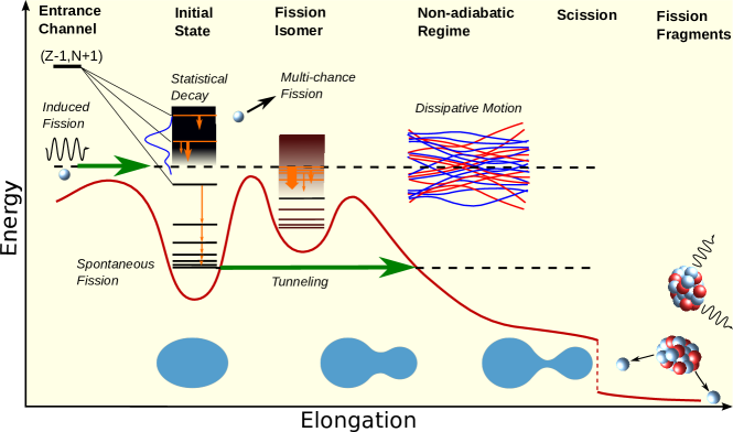
Figure 1: Schematic illustration of the main physics concepts at play in fission. Potential energy surfaces (in one dimension like here: a potential energy curve) play a key role in determining the spontaneous fission probabilities, as well as the identities of the fission fragments and their distribution. The level structure above the ground state (first minimum) and the fission isomer (second minimum) will impact the fission cross sections. What is called the descent from saddle to scission involves a very slow, diabatic motion characterized by multiple level crossings and conversion between collective and intrinsic energy.

Figure 1 summarizes the main physics concepts relevant in fission theory. The figure represents the variation of the total energy as a function of the elongation, with several pictorial illustrations of the nuclear shape along the way. As mentioned above, the very introduction of the notion of elongation, that is, deformation, requires invoking the phenomenon of spontaneous symmetry breaking at play in EDF theories. It also requires specifying a set of collective variables that will quantify this deformation. For the sake of simplicity, the figure was made by considering a single collective variable. The interplay between collective motion and intrinsic excitation, aka the dissipative motion of the system, is especially relevant beyond the second barrier. The point of scission, where the two fragments are formed, is represented here as a sharp drop in total energy.

2 Theoretical Models

As mentioned above, most microscopic approaches to fission are based on the nuclear energy density functional (EDF) framework Schunck (2019). The term energy density functional methods encompasses both a set of general many-body techniques such as the Hartree-Fock, BCS and Hartree-Fock-Bogoliubov theories, the QRPA or the generator coordinate method, and an approximation for the in-medium nuclear forces inside the nucleus. The many-body techniques offer an ansatz for the many-body wave function representing the nucleus, while the effective Hamiltonian, or energy functional, modeling nuclear forces, ensures that said ansatz “works” and allows reproducing nuclear observables such as binding energies, excited states, etc.

2.1 Energy Density Functional Theory

In all recent applications, the basic building block of the EDF approach is the Hartree-Fock-Bogoliubov (HFB) theory Valatin (1961), which provides a general method to determine an approximation of both the ground state and excited states for a many-body quantum system described by a product-state wave function. The HFB theory has been presented in great details in the review articles Valatin (1961); Mang (1975); Bender et al. (2003) as well as in several textbooks Blaizot and Ripka (1985); Ring and Schuck (2004); Schunck (2019) and below we will only give a very brief summary.

Hartree-Fock-Bogoliubov Theory

General Formalism - The HFB theory is most conveniently explained in the language of second quantization. We begin with a basis of single-particle states represented by a set of fermion creation and annihilation operators $(c_{m}^{\dagger},c_{m})$ with $m=1,\dots,+\infty$. Note that in practical applications, the single-particle basis is truncated to have only a finite number of terms $p$. This basis can be, for instance, associated with the eigenstates of the harmonic oscillator. The Bogoliubov transformation introduces a new set $(\beta_{\mu}^{\dagger},\beta_{\mu})$ of fermion operators,

$$\beta_{\mu} =\displaystyle\sum_{m}\left[U^{\dagger}_{\mu m}\,c_{m}+V^{\dagger}_{\mu m}\,c_{m}^{\dagger}\right],\vskip 6.0pt plus 2.0pt minus 2.0pt$$ (3)

$$\beta_{\mu}^{\dagger} =\displaystyle\sum_{m}\left[V^{T}_{\mu m}\,c_{m}+U^{T}_{\mu m}\,c_{m}^{\dagger}\right].$$ (4)

where $U$ and $V$ form the Bogoliubov matrix

$$\mathcal{W}=\left(\begin{array}[]{cc}U&V^{*}\\ V&U^{*}\end{array}\right).$$ (5)

The operators $\beta_{\mu}^{\dagger}$ and $\beta_{\mu}$ are the quasiparticle (q.p.) operators. In the HFB theory, one assumes that the many-body wave function can be represented as a product state of quasiparticle operators,

$$\ket{\Phi}=\prod_{\mu}\beta_{\mu}\ket{0},$$ (6)

where $\ket{0}$ is the particle vacuum. Quasiparticles can be interpreted as excitations of the system: $\beta_{\mu}^{\dagger}\ket{0}$ creates an excited state on top of the vacuum. The ansatz (6) thus translates the fact that the HFB ground state is a zero-excitation state.

Given the form (6) of the HFB wave function, the next step is to compute the total energy. For the sake of simplicity, we will only discuss the case where the energy is calculated as the expectation value of an effective Hamiltonian $\hat{H}_{\rm eff}$,

$$E=\frac{\braket{\Phi}{\hat{H}_{\rm eff}}{\Phi}}{\braket{\Phi}{\Phi}}.$$ (7)

We refer the interested readers to more complete presentations for the case where the energy is derived from an energy functional Schunck (2019). When the effective Hamiltonian reads $\hat{H}=\hat{T}+\hat{V}$ with $\hat{V}$ containing only two-body effective forces, the total energy becomes

$$E[\rho,\kappa,\kappa^{*}]=\sum_{ij}t_{ij}\rho_{ji}+\frac{1}{2}\sum_{ijkl}\bar{v}_{ijkl}\rho_{lj}\rho_{ki}+\frac{1}{4}\sum_{ijkl}\bar{v}_{ijkl}\kappa^{*}_{ij}\kappa_{kl}.$$ (8)

where $\rho$ is the one-body density matrix and $\kappa$ the pairing tensor defined as

$$\rho_{mn}=\frac{\braket{\Phi}{c_{n}^{\dagger}c_{m}}{\Phi}}{\braket{\Phi}{\Phi}},\qquad\kappa_{mn}=\frac{\braket{\Phi}{c_{n}c_{m}}{\Phi}}{\braket{\Phi}{\Phi}},\qquad\kappa_{mn}^{*}=\frac{\braket{\Phi}{c_{m}^{\dagger}c_{n}^{\dagger}}{\Phi}}{\braket{\Phi}{\Phi}},$$ (9)

and the matrix elements of the operators are $t_{ij}=\braket{i}{\hat{T}}{j}$ (kinetic energy) and $v{ijkl}=\braket{ij}{\hat{V}}{kl}$ (two-body potential). The notation $\bar{v}_{ijkl}=v_{ijkl}-v_{ijlk}$ indicate the antisymmetrization of all matrix elements. By construction, the degrees of freedom in the HFB theory are the matrix elements of the Bogoliubov transformation or, equivalently, those of the one-body density matrix and pairing tensor. They are determined by requiring that the total energy (8) be minimum with respect to their variations. This leads to the HFB equation, which takes the form of the commutator

$$\big{[}\mathcal{H},\mathcal{R}\big{]}=0,$$ (10)

where the HFB matrix $\mathcal{H}$ and generalized density $\mathcal{R}$ read

$$\mathcal{H}=\left(\begin{array}[]{cc}h&\Delta\\ -\Delta^{*}&-h^{*}\end{array}\right),\qquad\mathcal{R}=\left(\begin{array}[]{cc}\rho&\kappa\\ -\kappa^{*}&1-\rho^{*}\end{array}\right),$$ (11)

with $h_{ij}=t_{ij}+\sum_{kl}\bar{v}_{ikjl}\rho_{lk}$ is the mean field and $\Delta_{ij}=\frac{1}{2}\sum_{kl}\bar{v}_{ijkl}\kappa_{kl}$ the pairing field. Solving (10) determines completely the generalized density, hence $\rho$ and $\kappa$. Physical observables can be computed by taking the trace of the corresponding operator with the densities. In the simplest case of one-body operators $\hat{F}$, this means: $\braket{\hat{F}}=\mathrm{Tr}(\hat{F}\rho)=\sum_{ij}F_{ij}\rho_{ji}$. The expectation value of two- and $N$-body operators can be computed thanks to the Wick theorem Ring and Schuck (2004); Schunck (2019).

Constraints - As mentioned earlier in the introduction, the theoretical description of fission involves mapping out the variations of the total energy as a function of the deformation of the fissioning nucleus. In phenomenological models based on the macroscopic-microscopic method, this is achieved by parameterizing the nuclear shape; in the HFB theory, this requires seeking solutions of the HFB equation (10) with constraints on the expectation value of operators associated with the nuclear shape. The simplest example of such operators are the multipole moments (computed in the intrinsic frame of reference): $\hat{Q}_{\lambda\mu}=c_{\lambda\mu}r^{\lambda}Y_{\lambda\mu}$, where $c_{\lambda\mu}$ is a normalization constant and $Y_{\lambda\mu}$ are the spherical harmonics Varshalovich et al. (1988). Let us note $\{\hat{F}_{a}\}_{a=1,\dots,N}$ the set of $N$ operators on which expectation value we seek to impose a constraint. This can be achieved by the standard method of Lagrange parameters: instead of minimizing the total energy $E[\rho,\kappa,\kappa^{*}]$, we minimize instead $\mathcal{E}=E-\sum_{a}(\braket{\hat{F}_{a}}-\bar{F}_{a})$, where $\bar{F}_{a}$ is the target value for the constraint and $\braket{\hat{F}_{a}}=\mathrm{Tr}(\hat{F}_{a}\rho)$ the expectation value (here assuming a one-body operator only). It is straightforward to see that the HFB matrix is modified and becomes

$$\mathcal{H}=\left(\begin{array}[]{cc}h-\sum_{a}F_{a}&\Delta\\ -\Delta^{*}&-h^{*}+\sum_{a}F^{*}_{a}\end{array}\right),$$ (12)

where $F_{a}$ is now the matrix of the operator $\hat{F}_{a}$ in the single-particle basis. Even without specific constraints on the nuclear shape, this technique is needed to ensure the conservation of particle number in the HFB equation: choosing $\hat{F}_{a}\equiv\hat{N}$ ensures that HFB solution (6) has the right number of particles on average.

There are two main techniques to solve the HFB equation (10). As well known from basic quantum mechanics, if two operators commute, it is possible to find a common eigenbasis. One popular approach to solving the HFB equation thus involves recasting (10) into a non-linear eigenvalue problem which is solved iteratively. Alternatively, one may view the HFB equation as a minimization problem. By suitably parameterizing the HFB wave function thanks to the Thouless theorem, one can adapt gradient techniques to minimize the energy. These two techniques are discussed in details in Schunck (2019).

Spontaneous symmetry breaking - As mentioned above, the ansatz (6) for the HFB wave function implies that this wave function is not an eigenstate of the particle number operator $\hat{N}=\sum_{i}c_{i}^{\dagger}c_{i}$. Similarly, solving the HFB equation (10) with constraints on the expectation value of multipole moments in the intrinsic frame implies that the density matrix $\rho$ is not going to be rotationally invariant. Two fundamental symmetries of the nuclear Hamiltonian, particle number and rotational invariance, are thus broken in the HFB theory. This spontaneous symmetry breaking is a trademark of the EDF theory and one of the main reasons why, in practice, this approach provides an accurate model for atomic nuclei. As discussed extensively in Ring and Schuck (2004); Duguet (2014); Schunck (2019), the symmetry group $\mathcal{G}$ of the nuclear Hamiltonian reads

$$\mathcal{G}=T(3)\times SO(3)\times\Pi\times U(1)_{N}\times U(1)_{Z}\times SU(2)$$ (13)

where $T(3)$ is the Abelian Lie group of space translations associated with the conservation of the linear momentum; $SO(3)$ is the non-Abelian Lie group of space rotations associated with the conservation of angular momentum; $\Pi$ is the Abelian, finite and discrete group associated with reflection symmetry; $U(1)_{X}$ is the Abelian Lie group associated with the conservation of the number of particles ($X=Z$ for protons, $X=N$ for neutrons) and $SU(2)$ is the group associated with isospin symmetry. Saying that $\mathcal{G}$ is the symmetry group of the nuclear Hamiltonian means that for any element $g\in\mathcal{G}$ and the relevant unitary operator $\hat{U}(g)$, we have: $[\hat{U}(g),\hat{H}]=0$. The key feature of the EDF approach is to seek solutions to the HFB equation that can break any of these symmetries. By doing so, we explore a variational space that is richer and, as a consequence, can lower the total energy: the product state (10) contains correlations that would not be present otherwise and combined with suitably chosen effective Hamiltonian $\hat{H}_{\rm eff}$ gives a realistic approximation of the nuclear wave function. It is important to realize that the microscopic description of fission is entirely built upon this concept and the related mathematical framework. As of now, we do not have an alternative description of the phenomenon rooted, e.g., in the nuclear shell model or ab initio methods, where symmetries are never broken.

Energy functionals - The previous paragraphs summarized important general concepts of the EDF theory. In practical applications, one must specify the effective Hamiltonian $\hat{H}_{\rm eff}$ or, alternatively, the energy functional $E[\rho,\kappa,\kappa^{*}]$ in order to perform calculations. The Skyrme and Gogny energy functionals are among the most commonly used models for nuclear forces Bender et al. (2003); Stone and Reinhard (2007); Robledo et al. (2019); Schunck (2019). These functionals are derived from non-relativistic, two-body effective Hamiltonians. The Skyrme Hamiltonian is a local zero-range potential, i.e., of the type $\hat{V}(\mathbf{r}_{1},\mathbf{r}_{2})\delta(\mathbf{r}_{1}-\mathbf{r}_{2})$ with $\mathbf{r}_{1}$ and $\mathbf{r}_{2}$ the coordinates of the two nucleons; the Gogny Hamiltonian is a local, finite-range potential of the type $\hat{V}(\mathbf{r}_{1},\mathbf{r}_{2})$ where the dependency on $\mathbf{r}_{1}$ and $\mathbf{r}_{2}$ is proportional to $\exp\big{[}(\mathbf{r}_{1}-\mathbf{r}_{2})^{2}/\mu^{2}\big{]}$ with $\mu$ a typical length scale. Each of these Hamiltonian contains a central part, a density-dependent part that mocks up the effect of three-body forces and a spin-orbit part. In addition, both effective Hamiltonians contain a Coulomb potential. While the form (8) suggests that the same potential should be used to compute both the mean field energy (proportional to $\rho\rho$) and the pairing energy (proportional to $\kappa\kappa^{*}$), practitioners tend to adopt the following, more flexible (and less consistent) formula

$$E[\rho,\kappa,\kappa^{*}]=\sum_{ij}t_{ij}\rho_{ji}+\frac{1}{2}\sum_{ijkl}\bar{v}_{ijkl}^{\rho\rho}\rho_{lj}\rho_{ki}+\frac{1}{4}\sum_{ijkl}\bar{v}_{ijkl}^{\kappa\kappa}\kappa^{*}_{ij}\kappa_{kl}.$$ (14)

where the potential in the mean-field and pairing channel is different. In such cases, the matrix elements $\bar{v}_{ijkl}^{\kappa\kappa}$ of the pairing channel are typically computed from a simple pairing functional, e.g., a density-dependent zero-range pairing force Dobaczewski et al. (2002).

Multi-Reference Energy Density Functional

While the mechanism of spontaneous symmetry breaking discussed above seems at first sight ideal to describe the extreme deformation process that fission is, it also leads to the unintended consequences discussed in the introduction: all the quantum numbers associated with the broken symmetries of the group $\mathcal{G}$ are lost. This means that a deformed nucleus described by an HFB wave function of the type (6) cannot be labelled by angular momentum $JM$ and parity $\pi$, in addition to not being even associated with a fixed number of particles $Z$ and $N$. In fact, the single-reference EDF wave function can be written as the wave packet

$$\ket{\Phi}=\sum_{JM}\sum_{\pi}\sum_{ZN}c(Z,N,J,M,\pi)\ket{\Psi^{ZN}_{JM\pi}},$$ (15)

where $\ket{\Psi^{ZN}_{JM\pi}}$ is an eigenstate of the particle number operators (both protons and neutrons), of $\hat{J}^{2}$ and $\hat{J}_{z}$ and of the parity operator $\hat{P}$, with $c(Z,N,J,M,\pi)$ the coefficients of the expansion that depend on all the relevant quantum numbers. It is worth noting that the expansion (15) also applies to more phenomenological theories of fission such as the macroscopic-microscopic model. In fact, it is inherent to any theory relying on spontaneous symmetry breaking. In practice, the expansion(15) implies that the potential energy surface computed, e.g., at the HFB approximation, does not correspond to the nucleus $(Z,N)$ (even if one used constraints to enforce the average value of both $Z$ and $N$)), but to a superposition of different nuclei with different numbers of protons and neutrons. Similarly, one could introduce constraints on the average value $\braket{\hat{J}}$ of angular momentum to produce potential energy surface at different spins, but the resulting surfaces would be, strictly speaking, superpositions of surfaces at different $J$.

Projection Techniques - Quantum numbers can be recovered by projecting HFB solutions on the appropriate subspace of the Hilbert space. Starting with a symmetry-breaking HFB wave function $\ket{\Phi(g)}$, where $g$ is the parameter corresponding to some some continuous symmetry $S$ of the symmetry group $\mathcal{G}$, one can define a formal projector $\hat{P}_{S}$ as

$$\ket{\Psi}=\hat{P}_{S}\ket{\Phi(g)}=\int dg^{\prime}f(g^{\prime})\hat{R}(g^{\prime})\ket{\Phi(g)},$$ (16)

where $f(g^{\prime})$ is a weight function and $\hat{R}(g^{\prime})$ is the unitary transformation that changes the “orientation” $g$ of the wave function. Both $f(g^{\prime})$ and $\hat{R}(g^{\prime})$ depend on the symmetry group under consideration. For example, for the $U(1)_{N}$ group associated with particle number $N$, we have

$$U(1)_{N}:\quad\begin{array}[t]{rcl}\displaystyle\int dg^{\prime}&\equiv&\displaystyle\int_{0}^{2\pi}d\varphi,\vskip 6.0pt plus 2.0pt minus 2.0pt\\ \displaystyle f(g^{\prime})&\equiv&e^{+i\varphi N},\vskip 6.0pt plus 2.0pt minus 2.0pt\\ \displaystyle\hat{R}(g^{\prime})&\equiv&e^{-i\varphi\hat{N}}.\\ \end{array}$$ (17)

Note that in the expression of $f(g^{\prime})$, $N$ appears as a scalar while in that of $\hat{R}(g^{\prime})$, it is the operator. Another important example is angular momentum where

$$SO(3):\quad\begin{array}[t]{rcl}\displaystyle\int dg^{\prime}&\equiv&\displaystyle\frac{2J+1}{16\pi^{2}}\int_{0}^{2\pi}d\alpha\int_{0}^{\pi}d\beta\sin\beta\int_{0}^{4\pi}d\gamma,\vskip 6.0pt plus 2.0pt minus 2.0pt\\ \displaystyle f(g^{\prime})&\equiv&D_{MK}^{J*}(\alpha,\beta,\gamma),\vskip 6.0pt plus 2.0pt minus 2.0pt\\ \displaystyle\hat{R}(g^{\prime})&\equiv&e^{-i\alpha\hat{J}_{z}}e^{-i\beta\hat{J}_{y}}e^{-i\gamma\hat{J}_{z}}.\end{array}$$ (18)

Qualitatively, the effect of the projector is best understood in the case of rotations: it takes a given, deformed HFB solution $\ket{\Phi}$, rotates it in space by Euler angles $\Omega=(\alpha,\beta,\gamma)$ and combines the results to produce a rotationally-invariant wave function $\ket{\Psi}$. Details on the formalism, implementation and formal issues associated with projection techniques can be found in many review articles and textbooks; see Mang (1975); Ring and Schuck (2004); Schunck (2019); Bally and Bender (2021); Sheikh et al. (2021) for a short selection. In the context of fission theory, projection techniques have been applied only in a handful of cases, most notably to study the changes in the potential energy surfaces caused by the projection-induced correlation energy Bender et al. (2004); Hao et al. (2012); Marević and Schunck (2020). One of the most promising applications of projection has to do with the determination of the number of particles and spin distributions of fission fragments, which we will discuss later.

Configuration Mixing - As briefly mentioned earlier, spontaneous symmetry breaking allows exploring a richer variational space for the HFB solution $\ket{\Phi}$ which, however, remains an independent quasiparticle product state of the form (6). Following original ideas by Griffin and Wheeler, additional correlations can be encoded in the wave functions by performing a configuration mixing of different HFB states Griffin and Wheeler (1957), schematically,

$$\ket{\Psi}=\int d\mathbf{q}\,f(\mathbf{q})\ket{\Phi(\mathbf{q})},$$ (19)

where $f(\mathbf{q})$ is a weight function and $\ket{\Phi(\mathbf{q})}$ is the HFB state at point $\mathbf{q}$ in the collective space. The ansatz (19) is very general. In practice, the states $\ket{\Phi(\mathbf{q})}$ are known, e.g., by performing a series of HFB calculations, and only the weight functions $f(\mathbf{q})$ must be determined. This is done by inserting (19) into the many-body Schrödinger equation. This results in what is known as the Hill-Wheeler-Griffin equation

$$\int d\mathbf{q}\big{[}\mathcal{H}(\mathbf{q}^{\prime},\mathbf{q})-\mathcal{E}_{\mu}\mathcal{N}(\mathbf{q}^{\prime},\mathbf{q})\big{]}f_{\mu}(\mathbf{q})=0,$$ (20)

where $\mathcal{E}_{\mu}$ are the energies of the collective states $\ket{\Psi_{\mu}}$, $\mathcal{H}(\mathbf{q}^{\prime},\mathbf{q})$ is the energy kernel and $\mathcal{N}(\mathbf{q}^{\prime},\mathbf{q})$ is the norm kernel, given by

$$\mathcal{N}(\mathbf{q}^{\prime},\mathbf{q}) =\braket{\Phi(\mathbf{q})}{\Phi(\mathbf{q}^{\prime})},$$ (21)

$$\mathcal{H}(\mathbf{q}^{\prime},\mathbf{q}) =\braket{\Phi(\mathbf{q})}{\hat{H}}{\Phi(\mathbf{q}^{\prime})}$$ (22)

This configuration mixing is known in the literature as the generator coordinate method (GCM) and has a long history; we refer the interested reader to Wa Wong (1975); Reinhard and Goeke (1987); Bender et al. (2003); Ring and Schuck (2004) for further details. We will discuss the applications of the GCM framework to fission in the context of collective models.

2.2 Time-Dependent Density Functional Theory

Most of the preceding presentation of the EDF theory was focused on static, i.e., time-independent, nuclear properties. The EDF theory can also be extended to time-dependent phenomena through what we will refer, somewhat loosely, as time-dependent density functional theory (TDDFT) Bulgac (2013); Nakatsukasa et al. (2016). The starting point of TDDFT is the time-dependent many-body Schrödinger equation,

$$i\hbar\frac{\partial\ket{\Psi(t)}}{\partial t}=\hat{H}\ket{\Psi(t)},$$ (23)

where $\ket{\Psi(t)}$ is the exact, time-dependent many-body wave function of the system and $\hat{H}$ the nuclear many-boy Hamiltonian. The next step is to adopt an ansatz for the form of $\ket{\Psi(t)}$. In the time-dependent Hartree-Fock (TDHF) theory, we would enforce that $\ket{\Psi(t)}$ remains a product state of single-particle states at all times (=a Slater determinant); in the time-dependent Hartree-Fock-Bogoliubov (TDHFB) theory, we would similarly choose that $\ket{\Psi(t)}$ must be a Bogoliubov vacuum of the form (6) at all times (in other words: the operators $\beta_{\mu}$ are now time-dependent). The third step is to insert the chosen ansatz for the wave function into (23) and find a method to determine either the single-particle wave functions $\varphi_{k}(t)$ (TDHF) or the Bogoliubov matrices $U(t)$ and $V(t)$ (TDHFB). This step is not as straightforward as in the static case as shown in Blaizot and Ripka (1985); see also Balian and Vénéroni (1985, 1988); Lacroix et al. (2010); Lacroix (2011) for additional discussions. Here, we only recall the basic formula that are relevant for fission theory. In TDHF, the application of the variational principle leads to the following equation,

$$i\hbar\frac{\partial\rho}{\partial t}=\big{[}h[\rho(t)],\rho(t)\big{]},$$ (24)

where $\rho(t)$ is the time-dependent one-body density matrix and $h[\rho(t)]$ is the time-dependent mean field, which is a functional of the time-dependent density matrix. Although the TDHF equation is much simpler to solve numerically and was, historically, the first version of TDDFT applied to fission studies Negele et al. (1978); Umar et al. (2010); Simenel and Umar (2014), it has strong limitations: unless the calculation is initialized rather close to the scission point, or with an artificial boost in energy, the time-evolution of fissile nuclei such as ²⁴⁰Pu does not lead to fission Goddard et al. (2015, 2016). In order to achieve actual scission, pairing correlations play an essential role Scamps et al. (2015); Bulgac et al. (2016). For this reason, it is preferable to use either the TDHF+BCS theory Ebata et al. (2010); Scamps et al. (2012) or the fully-fledged TDHFB formalism. The TDHFB equation is formally similar to (24) as it reads

$$i\hbar\frac{\partial\mathcal{R}}{\partial t}=\big{[}\mathcal{H}(t),\mathcal{R}(t)\big{]},$$ (25)

where $\mathcal{R}(t)$ is the time-dependent generalized density matrix and $\mathcal{H}(t)$ the time-dependent HFB matrix; cf. (11). When setting the initial condition of the TDHFB equation near the saddle point of the potential energy surface (see Figure 1), the density of actinide nuclei will evolve toward two separated fragments as represented in Fig.2. In a sense, TDDFT generates fission events that are somewhat similar to Langevin trajectories.

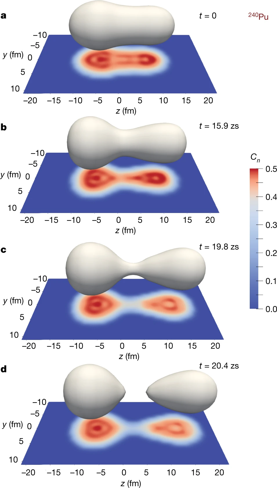
Figure 2: Real-time evolution of the one-body density of the ²⁴⁰Pu asymmetric fission from TDHF+BCS calculations. The 3D surface highlights the half-saturation density (0.08 fm^-3) isosurface whereas the projected color map corresponds to a localization function of the nucleons. Figures reproduced with permission from Scamps and Simenel (2018) courtesy of Scamps;

One of the key properties of TDDFT is that the total energy as computed from (8) (only, with time-dependent densities) is a constant of motion, $E(t)=E$. This means that if at $t=0$ the system is initialized in a static configuration $\mathbf{q}$ of energy $E_{0}=E(\mathbf{q}(t=0))$, corresponding to the top of the fission barrier, at later times it will have acquired an excitation energy $E^{*}=E_{0}-E(\mathbf{q}(t))$ since the potential energy tends to decrease with deformation. This property is the direct consequence of the fact that TDDFT simulates the diabatic evolution of the nucleus. It is a major advantage of TDDFT: when the fragments are formed at scission, the sharing of the prescission excitation energy will be done “automatically” based on nuclear forces and quantum many-body effects rather than empirical formulas based on physics intuition.

In spite of its many advantages, TDDFT also has limitations. By construction, it is designed to simulate the time-evolution of the expectation value $\braket{\hat{A}}$ of one-body observables (TDHF) or two-body observables (TDHFB, with some simplifications) Blaizot and Ripka (1985); Balian and Vénéroni (1985). It is not, however, well adapted to describe the fluctuations of these observables, that is, quantities $\sigma^{2}_{A}=\braket{\hat{A}^{2}}-\braket{\hat{A}}^{2}$; see discussions in Balian and Vénéroni (1984); Blaizot and Ripka (1985); Balian and Vénéroni (1992). This has practical consequences: when solving the TDHFB equation with a broad range of initial conditions at the beginning of the main fission valley in actinides, the resulting trajectories tend to bundle and converge to very similar solutions Bulgac et al. (2019a). In other words, TDHFB is very good at simulating the most likely fission but does a poor job at exploring less likely fragmentations. Different solutions have been proposed, including the stochastic mean field Ayik (2008); Lacroix and Ayik (2014); Tanimura et al. (2017) or adding empirical terms to simulate fluctuations and dissipation to the TDHFB equation Bulgac et al. (2019b). Another route, which we will discuss in the next section, consists in adopting a theoretical framework where collective correlations are explicitly included.

2.3 Collective Models

Time-dependent density functional does not assume the existence of collective variables. Although this may seems like an advantage of the approach since it removes some arbitrariness in defining what these variables should be, it turns out to be also a handicap to describe very collective phenomena like fission. The adiabatic time-dependent Hartree-Fock-Bogoliubov (ATDHFB) and the generator coordinate method with the Gaussian overlap approximation (GCM+GOA) incorporate collective variables $\mathbf{q}$ from the get-go, which allows them to probe collective correlations that may be out of reach of standard implementations of TDDFT.

Adiabatic Models

Early on, when solving the TDDFT equation was computationally intractable, there were many attempts to extract from the TDDFT equation a collective model that could be adapted to describing large-amplitude collective motion. The adiabatic time-dependent Hartree-Fock (ATDHF) and its extension to include pairing correlations (ATDHFB) provided many insights into such an approach Krieger and Goeke (1974); Brink et al. (1976); Villars (1977); Baranger and Veneroni (1978). Here, we only outline the main concepts of these theories and focus on ATDHFB; additional details can be found in the aforementioned references as well as the more recent reviews Nakatsukasa et al. (2016); Schunck (2019). In TDHFB, the system explores a large variational space during its evolution; in ATDHFB, one seeks to force the system to follow specific trajectories within a collective subspace $\Sigma$ of the entire Hilbert space which, ideally, is decoupled from the rest of the space. In the seminal paper of Baranger and Veneroni on ATDHF Baranger and Veneroni (1978), this was achieved by introducing a unitary transform of the TDHF density $\rho(t)$. In the case of ATDHFB, this transformation reads: $\mathcal{R}(t)\rightarrow e^{i\hat{\chi}(t)}\mathcal{R}(t)e^{-i\hat{\chi}(t)}$ where $\hat{\chi}(t)$ is a one-body operator that is supposed to be small. The transformed density is expanded up to second order in $\hat{\chi}$ together with the time-dependent HFB matrix, and the results are inserted into the TDHFB equation. Separating contributions that are time-odd from those that are time-even, we obtain the two coupled equations

$$i\hbar\dot{\mathcal{R}}^{(0)}&=\big{[}\mathcal{H}^{(0)},\mathcal{R}^{(1)}\big{]}+\big{[}\mathcal{H}^{(1)},\mathcal{R}^{(0)}\big{]},\\ i\hbar\dot{\mathcal{R}}^{(1)}=\big{[}\mathcal{H}^{(0)},\mathcal{R}^{(0)}\big{]}+\big{[}\mathcal{H}^{(0)},\mathcal{R}^{(2)}\big{]}+\big{[}\mathcal{H}^{(1)},\mathcal{R}^{(1)}\big{]}+\big{[}\mathcal{H}^{(2)},\mathcal{R}^{(0)}\big{]}.$$ (26)

These are the ATDHFB equations. The total collective energy of the system can be expressed as a function of the various components of the generalized density as

$$\mathcal{E}=\mathcal{V}+\frac{1}{2}\text{Tr}\left(\mathcal{H}^{(0)}\mathcal{S}^{(2)}\right)+\frac{1}{2}\text{Tr}\left(\mathcal{K}^{(1)}\mathcal{S}^{(1)}\right),$$ (27)

where $\mathcal{V}$, the collective potential energy, is in fact the HFB energy computed with $\mathcal{R}^{(0)}$. The kinetic energy term is the sum of the last two terms, which involve the matrices

$$\mathcal{S}^{(n)}=\left(\begin{array}[]{cc}\rho^{(n)}&\kappa^{(n)}\\ -\kappa^{(n)*}&-\rho^{(n)}\end{array}\right),\quad\mathcal{K}^{(n)}=\left(\begin{array}[]{cc}\Gamma^{(n)}&\Delta^{(n)}\\ -\Delta^{(n)*}&-\Gamma^{(n)}.\end{array}\right).$$ (28)

These are the $n^{\rm th}$ order term of the expansion of the TDHFB generalized density ($\mathcal{S}^{(n)}$) and HFB matrix ($\mathcal{K}^{(n)}$). Note that the diagonal elements of the $0^{\rm th}$ order term are slightly different since they look formally more like (11). In these expressions, all terms are time-dependent.

In principle, the ATDHFB equations should be solved self-consistently. In practice, however, the ATDHFB theory is mostly used to extract an expression for the collective inertia tensor. To this end, several approximations are invoked. The most important one consists in reducing the collective motion to a small set of collective variables $\mathbf{q}$ and assuming that

$$\dot{\mathcal{R}}_{0}=\sum_{\alpha}\frac{\partial\mathcal{R}_{0}}{\partial q_{\alpha}}\dot{q}_{\alpha}.$$ (29)

In other words, the variations of the generalized density are constrained within the manifold spanned by the vector $\mathbf{q}$. It is then possible to rewrite the total collective energy (27) as $\mathcal{E}=\mathcal{V}+\mathcal{K}$ where

$$\mathcal{K}=\frac{1}{2}\sum_{\alpha\beta}M_{\alpha\beta}\dot{q}_{\alpha}\dot{q}_{\beta}$$ (30)

is the total kinetic energy and $\mathsf{M}\equiv M_{\alpha\beta}$ is the collective mass tensor given by

$$M_{\alpha\beta}=\frac{\partial\mathcal{R}^{(0)}}{\partial q_{\alpha}}\mathcal{M}^{-1}\frac{\partial\mathcal{R}^{(0)}}{\partial q_{\beta}}.$$ (31)

Without additional approximations, the expression for $\mathsf{M}$ is not trivial as it involves the inverse $\mathcal{M}^{-1}$ of the QRPA matrix. The very first exact calculation of $\mathsf{M}$ has thus been reported only very recently Washiyama et al. (2021). Instead it is customary in most applications to fission to adopt the cranking approximation, where the QRPA matrix is reduced to its diagonal form (which can easily be inverted) and the derivatives in (31) are evaluated numerically. Analytical expressions requiring only HFB solutions at a single point $\mathbf{q}$ in the collective space can be obtained by using linear response theory to express all derivatives in terms of the moments of the constraint operators $\hat{Q}_{\alpha}$

$$M_{\alpha\beta}^{(-n)}=\sum_{\mu<\nu}\frac{\braket{\Phi(\mathbf{q})}{\hat{Q}_{\alpha}^{\dagger}}{\mu\nu}\braket{\mu\nu}{\hat{Q}_{\beta}}{\Phi(\mathbf{q})}}{(E_{\mu}+E_{\nu})^{n}},$$ (32)

where $\ket{\mu\nu}$ is a two-quasiparticle excitation of the state $\ket{\Phi(\mathbf{q})}$ and $E_{\mu}$ and $E_{\nu}$ are the energies of the q.p. $\mu$ and $\nu$. In that case, the collective mass tensor becomes

$$\mathsf{M}=\hbar^{2}\big{[}M^{(-1)}\big{]}^{-1}M^{(-3)}\big{[}M^{(-1)}\big{]}^{-1}$$ (33)

with the moments given by (32). The perturbative cranking approximation is numerically convenient but seems to have a large effect on the determination of spontaneous fission paths as reported in Sadhukhan et al. (2013); Giuliani and Robledo (2018).

The ATDHFB formula is probably the most commonly used in applications to fission, whether to compute spontaneous fission half lives or induced fission fragment distributions. Although it is known to give the correct collective mass at least in the case of translations, as applied in practical calculations the ATDHFB theory does not enforce a complete decoupling between collective and non-collective motion: doing so would not only require solving the ATDHFB equation (26)-(26) self-consistently rather than on a precomputed potential energy surface, it would also face conceptual problems caused by symmetry breaking; see discussion in Chapter 6 of Schunck (2019). The adiabatic self-consistent collective (ASCC) model solves many of these difficulties Matsuo et al. (2000); Hinohara et al. (2007, 2008) but has not been applied yet on realistic simulations of fission. Another limitation of the ATDHFB framework is that it assumes that at each point $\mathbf{q}$, the system is in its lowest energy state. Extensions of the formalism to include thermal excitations and diabatic motion have been proposed but not tested in practice Reinhard et al. (1986).

Generator Coordinate Method

The Hill-Wheeler-Griffin equation of the GCM is not solvable analytically and its physical content is not immediately visible. This motivated searches for suitable approximations. The Gaussian overlap approximation (GOA) has been the most popular Brink and Weiguny (1968); Onishi and Une (1975). It consists in assuming that the norm overlap is a generalized Gaussian function of $\mathbf{q}-\mathbf{q}^{\prime}$ of the type

$$\mathcal{N}(\mathbf{q},\mathbf{q}^{\prime})\propto\exp\left[-\frac{1}{2}\sum_{\alpha\beta}(q_{\alpha}-q^{\prime}_{\beta})G_{\alpha\beta}(q_{\beta}-q^{\prime}_{\beta})\right],$$ (34)

where $\mathsf{G}\equiv G_{\alpha\beta}$ is called the metric tensor (in the most general case, it can depend on $\mathbf{q}$), and that the energy kernel can be written

$$\mathcal{H}(\mathbf{q},\mathbf{q}^{\prime})=\mathcal{N}(\mathbf{q},\mathbf{q}^{\prime})h(\mathbf{q},\mathbf{q}^{\prime}),$$ (35)

where $h(\mathbf{q},\mathbf{q}^{\prime})$ is a polynomial of degree 2 for the collective variables $\mathbf{q}$ and $\mathbf{q}^{\prime}$, which is called the reduced Hamiltonian. The main advantage of the GOA is that it allows transforming the Hill-Wheeler-Griffin equation into a Schrödinger-like collective equation for the function $g(\mathbf{q})$ that is related to the weight function through

$$g(\mathbf{q})=\int d\mathbf{q}^{\prime}\,\mathcal{N}^{1/2}(\mathbf{q},\mathbf{q}^{\prime})f(\mathbf{q}^{\prime}).$$ (36)

The function $g(\mathbf{q})$ can be interpreted as a probability to be at point $\mathbf{q}$ in the collective space. The GCM+GOA provides a general framework to compute the collective inertia tensor and various zero-point energy corrections associated with the collective motion Reinhard and Goeke (1987). Indeed, after using the GCM ansatz (19) for the many-body wave function $\ket{\Psi}$ and inserting the GOA approximations (34)-(35), one can show (after some rather lengthy derivations presented in Ring and Schuck (2004); Krappe and Pomorski (2012)) that the expectation value of the total energy $\braket{\Psi}{\hat{H}}{\Psi}$ becomes

$$\braket{\Psi}{\hat{H}}{\Psi}=\int d\mathbf{q}g^{*}(\mathbf{q})\mathcal{H}_{\rm coll}(\mathbf{q})g(\mathbf{q}),$$ (37)

where the collective Hamiltonian $\mathcal{H}_{\rm coll}(\mathbf{q})$ reads

$$\mathcal{H}_{\rm coll}(\mathbf{q})=-\frac{\hbar^{2}}{2}\sum_{\alpha\beta}\frac{\partial}{\partial q_{\alpha}}B_{\alpha\beta}(\mathbf{q})\frac{\partial}{\partial q_{\beta}}+\mathcal{V}(\mathbf{q}).$$ (38)

In this expression, which corresponds to the special case of a constant metric $\mathsf{G}$, $\mathsf{B}=\mathsf{M}^{-1}$ is the collective inertia (the inverse of the collective mass) and $\mathcal{V}(\mathbf{q})$ is the collective potential. The collective potential is typically the sum of the HFB potential energy at point $\mathbf{q}$ and some zero-point energy corrections $\varepsilon_{\rm ZPE}(\mathbf{q})$. In a similar manner as for the ATDHFB theory, the calculation of the GCM+GOA collective mass and zero-point energy requires computing some derivatives with respect to the collective variables and dealing with the inverse of the QRPA matrix $\mathcal{M}$; see Schunck and Robledo (2016) for details. It is possible to adopt the same cranking and perturbative cranking approximation to simplify the calculations and make all quantities local to the point $\mathbf{q}$ in the coordinate space. In such cases, the collective mass and zero-point energy are given by

$$\mathsf{M}=4\mathsf{G}M^{(-1)}\mathsf{G},\qquad\varepsilon_{\rm ZPE}(\mathbf{q})=\frac{1}{2}\mathsf{G}\mathsf{M}^{-1},$$ (39)

with $M^{(-1)}$ the same moments defined above by (32). In its common implementations, the GCM+GOA suffers from the same limitations as the ATDHFB theories: it only includes quasiparticle vacuua at point $\mathbf{q}$ and, therefore, cannot handle diabatic motion. This could be remedied either by enlarging the collective space to include quasiparticle excitations as proposed in Bernard et al. (2011), or by developing a more general theory of quantum transport that combines the GCM with a finite-temperature formalism Dietrich et al. (2010).

The GOA can also be applied to provide a time-dependent collective model. When the ansatz (19) is inserted in the time-dependent many-body Schrödinger equation, the resulting equation defines the time-dependent generator coordinate method (TDGCM) Verriere and Regnier (2020). The GOA can then be applied to the TDGCM leading to the collective equation of motion

$$i\hbar\frac{\partial}{\partial t}g(\mathbf{q},t)=\left[-\frac{\hbar^{2}}{2}\sum_{\alpha\beta}\frac{\partial}{\partial q_{\alpha}}B_{\alpha\beta}(\mathbf{q})\frac{\partial}{\partial q_{\beta}}+\mathcal{V}(\mathbf{q})\right]g(\mathbf{q},t).$$ (40)

The right-hand side of this equation is exactly the same as (38), but the TDGCM+GOA equation now provides an evolution equation for the time-dependent probability of the system to be at a specific location $\mathbf{q}$ in the collective space at time $t$. Since the pioneering work of the CEA,DAM,DIF group at Bruyères-le-Chatel Berger et al. (1984); Berger (1986); Goutte et al. (2004), this technique has proven very successful to compute the distributions of fission fragments as we will see below.

3 Selected Results

3.1 Spontaneous Fission

As mentioned in the introduction, the description of spontaneous fission relies heavily on the concept of tunneling across multi-dimensional potential energy surfaces. Specifically, all realistic estimates of spontaneous fission half-lives published so far are based on the WKB formula to estimate the transmission coefficient through the barrier Landau and Lifshitz (1981). The half-life is then given by the inverse of the transmission coefficient times the number of assaults to the barrier per unit time $\nu$ and reads

$$\tau_{\rm SF}=\frac{1}{\nu}\exp\left(\frac{2}{\hbar}\int_{a}^{b}ds\sqrt{2B(s)(\mathcal{V}(s)-E_{0})}\right),$$ (41)

where $E_{0}$ is the ground-state energy and $\mathcal{V}$ the potential energy along the most likely fission path as parametrized by the curvilinear abscissa $s$. The quantity $B(s)$ is the collective inertia tensor that we have already mentioned several time. The integrand in (41) is the classical action, and it is integrated between the inner turning point $s=a$ and the outer turning point $s=b$. The formula (41) requires a collective space spanned by some variables $\mathbf{q}$, with a collective potential energy $\mathcal{V}(\mathbf{q})$ and a collective inertia tensor $\mathsf{B}(\mathbf{q})$. Since there are different models to compute these quantities (we mentioned the ATDHFB and GCM+GOA models) there will be a strong dependency of the calculated spontaneous fission half-lives on the model inputs – especially so since both the potential and inertia enter as an exponent. For example, systematic calculations show very large variations of $\tau_{\rm SF}$ depending on: (i) the model used to compute the inertia (ATDHFB or GCM) and the accompanying approximations (perturbative versus non-perturbative cranking) Sadhukhan et al. (2013); Giuliani et al. (2018) (ii) the model to compute the collective energy $\mathcal{V}$ Bernard et al. (2019) (iii) the type and number of collective variables, especially the role of pairing correlations Sadhukhan et al. (2014); Giuliani et al. (2014); Zhao et al. (2016), (iv) the prescription for the ground-state energy Staszczak et al. (2009); Giuliani et al. (2018).

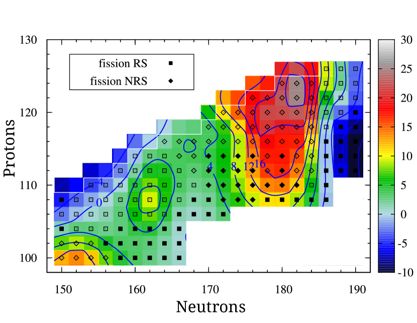
Figure 3: Logarithm of the spontaneous fission half-lives of heavy and superheavy even-even nuclei with the D1S Gogny functional. Nuclides where fission is the dominant decay mode are represented by filled symbols, those were $\alpha$ decay is dominant by open symbols. Squares indicate reflection-symmetric fission while diamonds indicate reflection-asymmetric fission. Figures reproduced with permission from Baran et al. (2015) courtesy of Warda; copyright 2015 by Elsevier.

In large-scale simulations, the spontaneous fission half-life is not computed from the most likely fission path but from the least-energy path. Finding the most likely fission path requires computing a $N$-dimensional collective space between the ground-state and the outer turning line and then selecting out of all possible trajectories the one that minimizes the classical action. The computational cost is substantial and for this reason, this method has not been applied to systematic calculations. Instead, such calculations are based on computing an effective one-dimensional fission path, typically parametrized by the axial quadrupole moment, and assume that such a path is a good approximation of the most likely fission path. Figure 3 shows a representative example such a global calculation of $\tau_{\rm SF}$ for even-even heavy and superheavy elements in the case of the Gogny energy functional Baran et al. (2015); similar systematics are also available for the Skyrme functional Staszczak et al. (2013). Although agreement with experimental data (where available) may not always be better than a few orders of magnitude, one should keep in mind that, because of the exponential factor in (41), half-lives are unforgiving tests of nuclear models. One of the advantages of microscopic methods is that they provide a consistent, rigorous and improvable framework to evaluate $\tau_{\rm SF}$. As computational capabilities increase, it should soon become possible to extract genuine least-action trajectories from multi-dimensional potential energy surfaces for an entire section of the nuclear chart (instead of a few isotopes) and compute $\tau_{\rm SF}$ with exact ATDHFB inertia and energy functionals properly calibrated to nuclear deformation properties. Even if the WKB approximation proves insufficient, there are already several other avenues worth exploring such as functional integral methods Levit (1980); Levit et al. (1980a, b); Puddu and Negele (1987); Levit (2021), instantons Skalski (2008); Brodziński and Skalski (2020), time-dependent Schrödinger with a complex absorbing potential Scamps and Hagino (2015), configuration-interaction approach Hagino and Bertsch (2020a, b).

While half-lives have been the focus of most studies of spontaneous fission, they are not the only observables in this process. Fission fragment distributions are also important, especially for applications to, e.g., nucleosynthesis modeling where fission fragments may re-enter the set of reactions forming heavy elements Vassh et al. (2020); Cowan et al. (2021). Such distributions also probe the influence of the entrance channel and/or the dependence of fission fragment distributions on the excitation energy of the nucleus. For example, neutron reactions on ²³⁹Pu lead to the fission of ²⁴⁰Pu with prescission energies of the order of 20-25 MeV, while the spontaneous fission of that same ²⁴⁰Pu happens at much lower prescission energies, of the order of 15-20 MeV. The determination of spontaneous fission fragment distributions can be decomposed in a two-step process: (i) the calculation of the tunneling probabilities to go from the ground state to the outer turning line and (ii) the evolution of the system from the outer turning line to scission. In Sadhukhan et al. (2016), the authors propose to use a semi-microscopic method based on combining tunneling probabilities computed with the WKB formula and microscopic potential energy and collective inertia, and a semi-classical Langevin evolution from outer turning line to scission.

A subsequent study showed that non-classical Langevin trajectories (where the energy may increase because of fluctuations) played an essential role in setting the tails of the fission fragment distributions, which correspond to very asymmetric fission. This is illustrated in Fig.4. The left top panel shows the outer turning line and scission line in a two-dimensional potential energy surface in ²⁴⁰Pu. The bottom left panel shows eleven different families of Langevin trajectories that originate from different initial points at the outer turning line. Most of the trajectories follow the slope of the potential energy surface, but a few (most notably numbers 3 and 4), are non-classical, in the sense that the energy along the trajectory may increase. This behavior is the direct consequence of the large fluctuation-dissipation term in the Langevin equation. What the right panel of the figure shows is that these non-classical trajectories give contributions to the very asymmetric part of the fission fragment distributions.

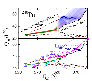
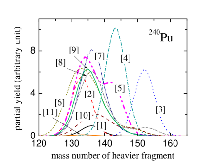
Figure 4: Left: Effective fission paths from the outer-turning line (brown dashed line) to scission (black dashed-dotted line) in ²⁴⁰Pu. Right: Contribution to the fission fragment distribution of each effective fission path Figures reproduced with permission from Sadhukhan et al. (2017) courtesy of Sadhukhan; copyright 2017 by APS.

3.2 Characterization of Fission Fragments

Number of Particles

For a long time, the number of particles in fission fragments was obtained in a semi-classical way by integrating the density of particles (proton, neutron or total density) in the regions of space associated with each fragment. If we note $z_{\rm N}$ the position along the $z$-axis where the density is the lowest between the two prefragments at scission, then the average number of particles in the right fragment would be

$$\bar{X}_{\rm R}=\int_{-\infty}^{+\infty}dx\int_{-\infty}^{+\infty}dy\int_{z_{\rm N}}^{+\infty}dz\,\rho_{X}(\mathbf{r})$$ (42)

where $\rho_{X}(\mathbf{r})$ is the density of particles $X=n,p$. As emphasized by the notation $\bar{\dots}$, the quantity thus computed is an average value. Among other things, it may not be an integer number. A much better prescription based on particle number projection techniques was proposed originally in Simenel (2011). The basic idea is to use the formalism very briefly outlined above with the following modification: the particle number operator is replaced by

$$\hat{X}_{\rm R}=\sum_{\sigma}\int d^{3}\mathbf{r}\,H(z-z_{\rm N})c^{\dagger}(\mathbf{r},\sigma)c(\mathbf{r},\sigma)$$ (43)

where $H(z-z_{\rm N})$ is the Heaviside function Abramowitz and Stegun (1964) and $c^{\dagger}(\mathbf{r},\sigma)$ creates a particle at point $\mathbf{r}$ with spin projection $\sigma$. By construction, the operator (43) counts the number of particles in the right fragment only, and it is easy to check that its expectation value is $\braket{\hat{X}_{\rm R}}=\bar{X}_{\rm R}$ as defined in (42). From the definition (16) specialized to the case (17) with the operator (43), we can then introduce the projection operator $\hat{P}^{(\rm R)}_{\rm X}(X_{\rm R})$ that extracts the probability that a wave function contains $X_{\rm R}$ particles in the right fragment. This allows us to define the probability to find $X_{\rm R}$ particles at point $\mathbf{q}$ in the collective space, given a total number of particles $X$ in the compound nucleus

$$\mathbb{P}(X_{\rm R}|X,\mathbf{q})=\frac{\braket{\Phi(\mathbf{q})}{\hat{P}^{(\rm R)}_{\rm X}(X_{\rm R})\hat{P}_{\rm X}(X)}{\Phi(\mathbf{q})}}{\braket{\Phi(\mathbf{q})}{\hat{P}_{\rm X}(X)}{\Phi(\mathbf{q})}}$$ (44)

An example of this probability is represented in Fig. 5 for different scission configurations of the compound nucleus ²³⁶U formed in the thermal reaction ²³⁵U(n,f). One can notice the case of the $(325,40)$ configuration (the numbers represent, respectively, the average quadrupole moment $\braket{\hat{Q}_{20}}$ [b] and average octupole moment $\braket{\hat{Q}_{30}}$ [b^3/2] of the configuration): the probability shows a clear odd-even staggering. This effect has been observed experimentally in the charge distributions Ehrenberg and Amiel (1972); Amiel and Feldstein (1975); Mariolopoulos et al. (1981); Bocquet and Brissot (1989) and could only be reproduced theoretically by introducing ad hoc parameters. Results such as the ones shown in Fig. 5 suggest that PNP may be the key ingredient needed to truly predict the odd-even staggering of charge distributions.

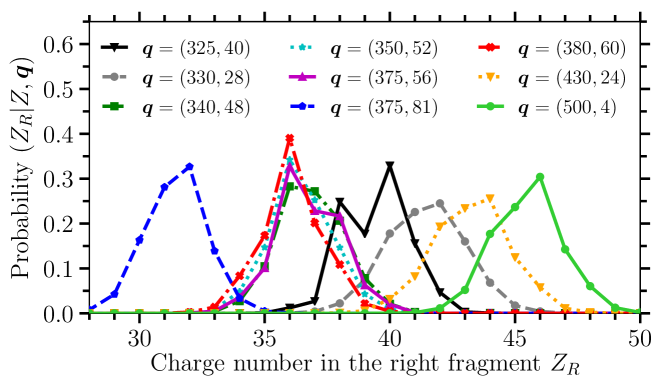
Figure 5: Probability distribution $\mathbb{P}(Z_{\rm R}|Z,\mathbf{q})$ of Eq. (44) that a single scission configuration $\mathbf{q}$ contains $Z_{\rm R}$ protons. Each curve corresponds to different scission configuration for the thermal fission of ²³⁵U(n,f). Figures reproduced with permission from Verriere et al. (2021) courtesy of Verriere; copyright 2021 by APS.

The first application of particle number projection in the fragments was done in Scamps et al. (2015). The formalism was presented in more details in Verrière et al. (2019) and was applied for the first time in the calculation of primary fission fragment charge, mass and isotopic distributions in Verriere et al. (2021). This technique has several advantages. First, it can be applied to phenomenological models based, e.g., on the macroscopic-microscopic model. The only ingredient needed is a set of single-particle levels associated with each configuration. Second, the method guarantees that the fragments will have an integer number of particles – as nature tells us. Finally, by substituting at each scission point a single pair of average numbers $(\bar{Z}_{\rm R},\bar{N}_{\rm R})$ by a two-dimensional probability distribution function $\mathbb{P}(Z_{\rm R},N_{\rm R}|Z,N,\mathbf{q})$, which is equal to $\mathbb{P}(Z_{\rm R}|Z,\mathbf{q})\times\mathbb{P}(N_{\rm R}|N,\mathbf{q})$ if calculations do not account for isospin mixing, the method produces much more realistic estimates of which fragments are populated. We will show later how this technique can be applied to compute isotopic yields $Y(Z,A)$ of neutron-induced fission reactions.

Deformations

As mentioned during the presentation of the formalism of the HFB theory, the deformation of the nuclear shape in EDF approaches is set by imposing constraints on the expectation value of suitable operators. This can be viewed as somewhat equivalent to macroscopic-microscopic methods, where the nuclear shape is parametrized with a set of parameters in such a way as to cover the range of shapes relevant in fission. The big difference between the two approaches, however, concerns the deformations that are not enforced specifically in the calculation. In macroscopic-microscopic models, two options are possible: if the shape parametrization has a finite number of parameters, as in most applications of fission, then any shape not represented by this parametrization can not be included in the calculation; if the parametrization has an infinite number of parameters, as in the multipole expansion of the nuclear radius, then all parameters not set explicitly are zero by default. In contrast, the variational principle at play in the EDF approach ensures that all multipole moment expectation values $\braket{\hat{Q}_{\lambda\mu}}$ that are not explicitly set by the user will automatically take whichever value minimizes the total energy. When computing potential energy surfaces, this property can turn into a curse as it is the reason why discontinuities appear in the surface Dubray and Regnier (2012). However, the same property turns into a blessing when looking at the properties of the fragments at scission.

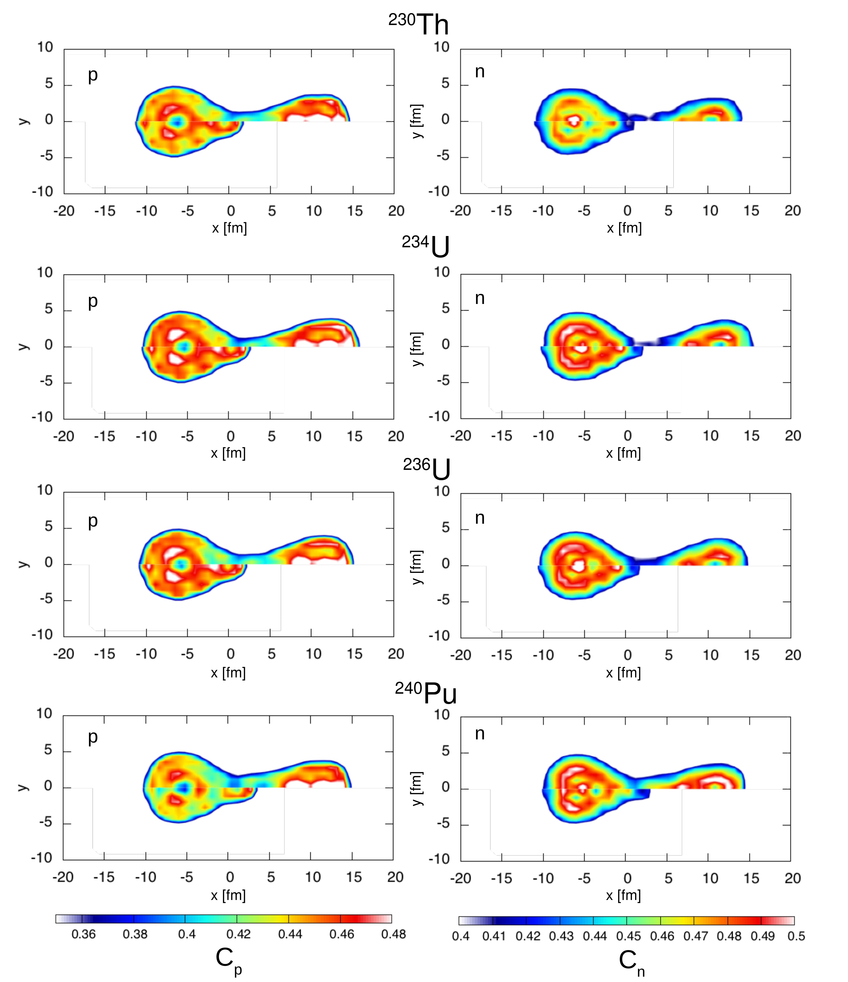
Figure 6: Identification of the heavy pre-fragment in the asymmetric fission of major and minor actinides. The figure compares the localization functions of the fissioning nucleus at scission (upper half of the contour plot in each frame) with that of the octupole deformed ¹⁴⁴Ba (lower-half of the contour plots) and highlights the role of octupole shell effects to determine the number of particles in the fragments. Figures reproduced with permission from Scamps and Simenel (2018) courtesy of Scamps; copyright 2021 by Nature.

Figure 6 shows the localization functions of the left and right fragments of several actinide nuclei at scission Scamps and Simenel (2018). The localization function is a visual indicator of not only the spatial profile of a density but also of it shell structure Reinhard et al. (2011). The figure compares the proton $C_{p}$ and neutron $C_{n}$ localization functions of the fissioning nucleus and the one of the octupole-deformed fragment ¹⁴⁴Ba, and shows that the heavy fragment in the most likely fragmentation tends to be octupole-deformed. The results reported in Scamps and Simenel (2018) explained for the first time why the peak of the fission fragment in actinides was not centered around ¹³²Sn as would be expected if only spherical shell effects, which are maximum at $Z=50$ and $N=82$, were active in the fission fragments. Instead, they suggested that the peak of the distribution is slightly shifted toward heavier $Z$ and $N$ value because of the competition with octupole shell effects, which are maximum for $Z=56$ and $N=88$ Butler and Nazarewicz (1996). These results were only possible because in EDF calculations, the deformation of the fragments is not set beforehand but is an outcome of the variational calculation: fragments may be spherical, quadrupole-deformed or octupole-deformed depending on their number of protons and neutrons. This is a compelling illustration of the predictive power of microscopic methods.

Spin Distributions

The prediction of the spin distributions of fission fragment is another, quite recent success of microscopic methods based on the EDF approach. The large number of photons emitted during the deexcitation of fission fragments is experimental evidence that fragments have a rather broad spin distribution. Until recently, the functional form of the spin distributions was based on the statistical model and read Bloch (1954)

$$p(J)\propto(2J+1)\exp\left[-\frac{1}{2}\frac{(J+\tfrac{1}{2})^{2}}{\sigma^{2}}\right],$$ (45)

where $\sigma$ is called the spin-cutoff parameter and is proportional to the expectation value $\braket{\hat{J}^{2}}$ of the total angular momentum in the system Madland and England (1977); Bertsch et al. (2019). In all deexcitation models of the nucleus, the parameter $\sigma$ is adjusted, together with other parameters pertaining to the decay, to match experimental data. Recent extensions of angular momentum projection in the fission fragments suggest that this parameter could be computed directly, or that (45) itself could be extracted from the projection on good $J$ of scission configurations Bulgac et al. (2021); Marević et al. (2021).

The extraction of the probability distribution (45) is analogous to the case of particle number. It is based on the angular momentum projection techniques of the MR-EDF theory presented earlier. Following Sekizawa (2017), one can define an angular momentum operator kernel acting only in the right fragment as

$$\mathbf{J}^{F}(\mathbf{r},\sigma)=H^{*}(z-z_{N})\mathbf{J}(\mathbf{r},\sigma)H(z-z_{N}),$$ (46)

where $\mathbf{J}(\mathbf{r},\sigma)=\mathbf{L}(\mathbf{r})+\mathbf{S}(\sigma)$ is the usual angular momentum operator acting on both spatial and spin coordinates and $H(z-z_{N})$ is, as before, the Heaviside step function. Assuming that the $z$-axis of the fissioning nucleus intrinsic frame is the axis of elongation, the center of mass of each fragment is located at $\mathbf{r}_{\text{CM}}^{F}=(0,0,z_{\text{CM}}^{F})$. Therefore, we must take $\mathbf{r}\rightarrow\mathbf{r}-\mathbf{r}_{\text{CM}}^{F}$ in (46) to determine the components of the angular momentum with respect to the center of mass of each fragment. To project on angular momentum in the fragments, the rotation operator of (18) must be defined with the components of the operator (46). The probability of finding spin $J$ in the fragment F at the scission configuration $\mathbf{q}$ is then

$$|c_{J}{\rm(F)}|^{2}=\frac{2J+1}{16\pi^{2}}\int_{0}^{2\pi}d\alpha\int_{0}^{\pi}d\beta\sin\beta\int_{0}^{4\pi}d\gamma\braket{\Phi(\mathbf{q})}{\hat{R}^{\rm(F)}(\Omega)}{\Phi(\mathbf{q})}.$$ (47)

In the two applications of this technique reported so far Bulgac et al. (2021); Marević et al. (2021), only axially-symmetric scission configurations were considered, which reduced the full rotation operator to a rotation around the $y$-axis of the reference frame: $\hat{R}^{\rm(F)}(\Omega)\rightarrow\hat{R}_{y}^{\rm(F)}(\beta)$. Just like in the case of particle number projection, the only ingredient to the method is a set of single- or quasi-particle states at scission making this technique applicable to macroscopic-microscopic models.

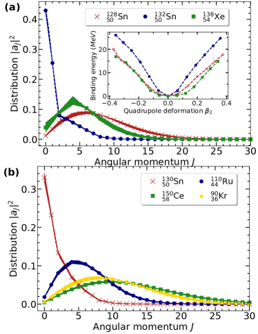
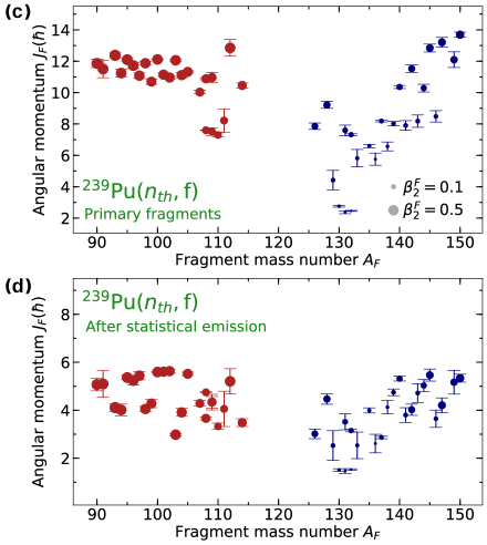
Figure 7: Left column: spin distribution of several heavy fragments in the fission of ²⁴⁰Pu. Panel (a) highlights that nuclei that are spherical in their ground state may be substantially deformed at scission, which completely changes their spin distribution. Panel (b) illustrates that, on average, the spin of the light fragment is larger than the one of the heavy fragment. Right column: Average spin $\langle J\rangle(A)$ as a function of the mass of the fragment. Panel (c) shows the result before any emission of particle, while panel (d) shows the results after emission of neutrons and statistical photons. Figures reproduced with permission from Marević et al. (2021) courtesy of Marevic; copyright 2021 by APS.

Figure 7 shows an example of such calculations for the benchmark case of ²⁴⁰Pu. Panel (a) shows the spin distribution for three isotopes near the doubly-magic ¹³²Sn nucleus. As recalled in the inset frame, all three isotopes are spherical in their ground state; at scission, however, their deformation can be different. While ¹³²Sn is still almost spherical, which manifests itself by a sharply peaked distribution around $J=0$, the distribution of both ¹²⁸Sn and ¹³⁸Xe has a relatively large spread extending up to $J=20\hbar$ for Xenon: this is indicative of a rather substantial deformation for that nucleus. Panel (b) highlights that the spin distribution of the fragments can vary substantially and, most importantly, that it does not depend only on the mass of the nucleus as often assumed in semi-empirical models of deexcitations Litaize and Serot (2010); Verbeke et al. (2018); Talou et al. (2021): the curves for ¹⁵⁰Ce and ⁹⁰Kr are very similar, yet the latter is 50% lighter than the former. Panels (c) and (d) on the right shows a systematics of the average spin of the fragments, that is, the quantity $\braket{J}$ defined through $\braket{J}(\braket{J}+1)=\sum_{J}|c_{J}{\rm(F)}|^{2}J(J+1)$, as a function of the mass of that fragment. The size of each circle represents the quadrupole deformation $\beta_{2}$ of the fragment and the error bar the uncertainty of the calculation. Panel (c) shows $\braket{J}$ for the primary fragments, i.e., before any emission of particles take place; panel (d) shows the same quantity after neutrons and statistical photons have been emitted. The statistical deexcitation was simulated with the code FREYA Verbeke et al. (2018). These results qualitatively reproduce (without adjustable parameters) recent experimental measurements Wilson et al. (2021).

The results reported in Fig. 7 were extracted from static calculations: angular momentum projection (in the fragments) was applied on HFB solutions corresponding to a large number of scission configurations Marević et al. (2021). While this allows extracting trends of $\braket{J}$ as a function of the mass or charge of the fragment, the downside of this approach is that the fragments are not fully separated and are “cold”: all their excitation energy is in the form of deformation energy. In Bulgac et al. (2021), the very same AMP technique was applied on the TDHFB solution for the most likely fission. As emphasized earlier, the total energy is a constant of motion in TDHFB simulations, hence the fragments have the right amount of excitation energy at scission. Interestingly, the spin distributions extracted from such “hot” fragments after full separation are very similar to the results obtained in “cold” fragments just before scission. This suggests that, as the shape of the fragments relax after the fragments separate, some deformation energy may be transferred into thermal excitation energy or, more rigorously, that the quantum fluctuations of $J$ induced by the large deformations are converted into statistical fluctuations Egido (1988).

Excitation Energy

The large number of emitted particles during the fission process is evidence that fission fragments are highly excited upon their formation. This simple fact can also be inferred from the energy balance of the fission reaction

$${\rm TXE}+{\rm TKE}+M(Z_{\rm H},N_{\rm H})+M(Z_{\rm L},N_{\rm L})=M(Z,N)+S_{n}(Z,N)+E_{n},$$ (48)

where $M(Z,N)$ is the mass of the nucleus $(Z,N)$, $S_{n}(Z,N)$ the one-neutron separation energy in the nucleus $(Z,N)$, $E_{n}$ the energy of the incident neutron in the center of mass frame, TXE the total excitation energy available to both fragments, and TKE the total kinetic energy of the fragments. In the case of spontaneous fission, there is no incident neutron: $S_{n}=E_{n}=0$. Similarly, for photofission (fission induced by photons), $S_{n}=0$ and $E_{n}\equiv E_{\gamma}$. In the fission of actinides, the mass of nearly all fission fragments is known with excellent precision, as is the mass of fissioning nucleus and its one-neutron separation energy. Measurements of TKE indicate that this quantity is in the range 150–190 MeV. It is then easy to find that the total excitation energy, as indicated from relation (48), is of the order of 30–50 MeV. To take an example: in the thermal neutron-induced fission of ²⁴⁰Pu, we have $Z=94$ and $N=146$, $E_{n}=0$ MeV and $S_{n}=8.31$ MeV. Let us consider the pair of fragments ¹³²Sn and ¹⁰⁸Ru: the TKE is ${\rm TKE}(A=132)=183.15$ MeV Tsuchiya et al. (2000). Based on the values of all nuclear masses Wang et al. (2021), we find ${\rm TXE}=36.01$ MeV. This energy must be distributed between the fragments. In approaches based on identifying scission configurations from a potential energy surface, this problem is not easy to solve because, as recalled in the previous section, the fragments are cold by construction. For this reason, the energy is usually shared based on a statistical formula that depends on the deformation (at scission) and level density of each fragment Schmidt and Jurado (2011); Albertsson et al. (2020). In microscopic theories, this approach is complicated by the fact that estimates of quantities such as the energy, number and particles, etc., in the fragments are dependent on the degree of entanglement between them Younes and Gogny (2011); Schunck et al. (2014, 2015).

Time-dependent DFT offers a very appealing solution to these problems. Recall that TDDFT equations simulate a complete fission event while, at the same time, conserving the total energy. If we wait long enough when running the simulation, we will reach the point where the two fragments are well separated with only the Coulomb force acting between them; see Fig. 2. The energy balance reads $E_{0}=E_{\rm H}(t)+E_{\rm L}(t)+E_{\rm int}(t)$, where $E_{0}=E(t=0)$ is the total, conserved energy of the system, $E_{\rm H,L}(t)$ is the time-dependent energy of the heavy/light fragment and $E_{\rm int}(t)$ is the interaction energy between them. At late times, or large distances between the two fragments, this interaction energy reduces to the total kinetic energy which is easily obtained from TDDFT evolution Simenel and Umar (2014); Tanimura et al. (2015). From that same evolution, we can extract the density matrix $\rho_{\rm H,L}(t)$ and pairing tensor $\kappa_{\rm H,L}(t)$ of each fragment and therefore calculate their total energy directly. Subtracting the ground-state binding energy of each fragment gives the excitation energy $E^{*}{\rm H,L}$. Estimates of both TKE and the $E^{*}{\rm H,L}$ have been obtained for the case of neutron-induced fission of ²³⁹Pu and agree rather well with experimental measurements Bulgac et al. (2016, 2019a). They also suggest that, at least for the most likely fission, the heavy fragment tends to have a lower internal temperature than the light one Bulgac et al. (2019a, 2020). Note that the shape relaxation of the fragments and the large Coulomb interaction at scission complicate this picture since they lead to the excitation of giant resonances, which in turn imply that the energy of each fragment is not constant over time Simenel and Umar (2014); Bulgac et al. (2020).

3.3 Distribution of Fission Fragments

The previous sections highlighted how microscopic methods based on the EDF approach can provide valuable insights on the properties of the fission fragments at the time of their formation, hence informing statistical models of deexcitation. Another piece of information that is crucial to model this decay is the relative population of each fission fragment. As mentioned in the introduction, this quantity is represented by the fission fragment distributions $Y(A)$ (mass distribution) $Y(Z)$ (charge distribution), and $Y(Z,A)$ (isotopic yields). Since the charge and mass of the fission fragments can be mapped onto the values of collective variables, predicting the relative population of the fragments is, to some extent, equivalent to predicting the population of specific points $\mathbf{q}$ of the collective space. The TDGCM is especially well suited to such a purpose, since the quantities $|g(\mathbf{q},t)|^{2}$ can precisely be interpreted as probabilities of occupation at point $\mathbf{q}$ and time $t$.

The formalism to extract the distributions from a TDGCM+GOA evolution was presented in Goutte et al. (2004); Regnier et al. (2016); Verriere et al. (2021), we only recall below the most important elements of the calculation. The (primary) yield of a fragment $(Z_{\rm f},N_{\rm f})$ is the probability

$$Y(Z_{\rm f},N_{\rm f})=100\big{[}\mathbb{P}(Z_{\rm f},N_{\rm f}|Z,N)+\mathbb{P}(Z-Z_{\rm f},N-N_{\rm f}|Z,N)\big{]},$$ (49)

where $\mathbb{P}(Z_{\rm f},N_{\rm f}|Z,N)$ is the probability that the right fragment has $Z_{\rm f}$ protons and $N_{\rm f}$ neutrons and the compound nucleus has $Z$ protons and $N$ neutrons. We assume that this probability is given by

$$\mathbb{P}(Z_{\rm f},N_{\rm f}|Z,N)\propto\int d\xi\,F(\xi)\mathbb{P}(Z_{\rm f},N_{\rm f}|Z,N,\mathbf{q}(\xi))$$ (50)

where $\mathbb{P}(Z_{\rm f},N_{\rm f}|Z,N,\mathbf{q}(\xi))$ is the analogue of the probability (44) and quantifies the probability that there is $Z_{\rm f}$ protons and $N_{\rm f}$ neutrons in the right fragment at the scission configuration $\mathbf{q}$. Here, we assume that the set of all scission configurations can be parametrized by the coordinate $\xi$ forming the scission “line” $\mathcal{S}\equiv\{\mathbf{q}(\xi)\}_{\xi}$. The quantity $F(\xi)$ is the time-integrated flux of the collective wave packet through this scission line. It is obtained by solving the TDGCM+GOA equation (40), defining the current $\mathbf{J}(\mathbf{q},t)$ from the function $g(\mathbf{q},t)$, computing the instantaneous flux of that current through the scission line and, finally, integrating it over time; we refer to Verriere et al. (2021) and references therein for further details.

Figure 8: Isotopic yields $Y(Z_{f},A_{f})$ for the reaction ²³⁹Pu(n,f) for different incoming neutron energies $E_{n}$. Particle number projection in both the fragments and the fissioning nucleus is used in each scission configuration. Symmetric fission becomes more probable with increasing excitation energy. Figures reproduced with permission from Verriere et al. (2021) courtesy of Verriere; copyright 2021 by APS.

In neutron-induced fission, each energy $E_{n}$ of the incident neutron corresponds to a different excitation energy of the fissioning nucleus. This excitation energy is used to fix the energy of the collective wave packet, given as

$$E_{\rm coll}(t)=\int d\mathbf{q}\,g^{*}(\mathbf{q},t)\left[-\frac{\hbar^{2}}{2}\sum_{\alpha\beta}\frac{\partial}{\partial q_{\alpha}}B_{\alpha\beta}(\mathbf{q})\frac{\partial}{\partial q_{\beta}}+V(\mathbf{q})\right]g(\mathbf{q},t).$$ (51)

In the TDGM+GOA, the total energy is also a constant of motion. Therefore, one can simulate the evolution of the fission fragment distributions with the energy of the incident neutron simply by changing the value of the initial TDGCM+GOA collective energy. The first results for both ²³⁹Pu(n,f) and ²³⁵U(n,f) were reported in Younes and Gogny (2012) and nicely reproduced the expected trend that symmetric fissions becomes enhanced as the neutron energy increases. Figure (8) shows another, more precise example of such calculations. Here, particle number projection in the fission fragment was applied to obtain a more realistic estimate of the particle number content (the probabilities $\mathbb{P}(Z_{\rm f},N_{\rm f}|Z,N,\mathbf{q}(\xi))$) of each scission configuration. The TDGCM+GOA equation was then solved with the code FELIX Regnier et al. (2018) to compute the isotopic yields in the case of ²³⁹Pu(n,f) reaction as a function of the incident neutron energy. The figure clearly shows the expected trend of enhanced symmetric fission

4 Conclusions

While nuclear fission has been studied for over eighty years, our understanding of the process remains fragmentary. Phenomenological models are invaluable for large-scale computations and the flexibility that their many adjustable parameters offer. However, improving these models require deeper insights into the quantum many-body features of the fission process, which only microscopic theories are capable of delivering. Currently, the only class of microscopic methods that are capable of computing actual fission observables are based on the general framework of the nuclear energy density functional theory. Essential tools include: the Hartree-Fock-Bogoliubov theory, which provides sets of symmetry-breaking many-body states used to generate potential energy surfaces and extract quantities such as fission barriers, fission paths and tunnelling probabilities; collective models based on the adiabatic approximation to large-amplitude collective motion or the generator coordinate method, which encode collective correlations that are especially important to extract the collective inertia tensor (used in the calculation of tunnelling probabilities) as well as to probe the entire phase space of fission; time-dependent density functional theory, which simulates directly fission events and can give rather good estimates of the initial conditions of the fission fragments upon their formation.

In the short to medium term, the recent work on projection techniques as a tool for estimating quantities such as the number of particles or spin distributions of the fragments will certainly be generalized and combined with various time-dependent descriptions to provide complete characterization of fission fragments before their deexcitation. Steady increase in computational capabilities will allow removing several of the approximations commonly used when implementing EDF methods, be they the small number of degrees of freedom, the small size of model space, etc. Methods borrowed from the areas of machine learning will help quantify theoretical uncertainties in predictions of fission observables and generate energy functionals with better calibrated deformation properties. Akin to a sophisticated Lego game, several of the theoretical tools briefly reviewed in this chapter could, potentially, be combined with one another, e.g., TDGCM and TDDFT. Many of these possibilities have been discussed in a recent white paper by the nuclear theory community Bender et al. (2020).

Taking the longer view, the playground of microscopic methods has so far been largely confined to the deformation phase of the fission process, that is, the evolution of the nucleus to the point of scission. The problem of fission cross sections, which is related to the determination of the entrance channel and the competition between fission and other decay modes, is still being addressed with semi-phenomenological methods. Switching to a microscopic approach would involve merging theories of nuclear structure and nuclear reactions.

References

- Hahn and Strassmann (1938) O. Hahn and F. Strassmann, Naturwiss. 26, 755 (1938).
- Hahn and Strassmann (1939) O. Hahn and F. Strassmann, Naturwiss. 27, 11 (1939).
- Meitner and Frisch (1939) L. Meitner and O. R. Frisch, Nature 143, 239 (1939).
- Bohr and Wheeler (1939) N. Bohr and J. A. Wheeler, Phys. Rev. 56, 426 (1939).
- Krappe and Pomorski (2012) H. Krappe and K. Pomorski, Theory of Nuclear Fission (Springer, 2012).
- Schunck and Robledo (2016) N. Schunck and L. M. Robledo, Rep. Prog. Phys. 79, 116301 (2016).
- Andreyev et al. (2017) A. N. Andreyev, K. Nishio, and K.-H. Schmidt, Rep. Prog. Phys. 81, 016301 (2017).
- Schmidt and Jurado (2018) K.-H. Schmidt and B. Jurado, Rep. Prog. Phys. 81, 106301 (2018).
- Younes et al. (2019) W. Younes, D. M. Gogny, and J.-F. Berger, A Microscopic Theory of Fission Dynamics Based on the Generator Coordinate Method, vol. 950 of Lecture Notes in Physics (Springer International Publishing, Cham, 2019), ISBN 978-3-030-04422-0.
- Younes and Loveland (2021) W. Younes and W. D. Loveland, An Introduction to Nuclear Fission (Springer, 2021), ISBN 978-3-030-84591-9.
- Weinberg (1990) S. Weinberg, Phys. Lett. B 251, 288 (1990).
- Machleidt and Sammarruca (2016) R. Machleidt and F. Sammarruca, Phys. Scr. 91, 083007 (2016).
- Hammer et al. (2020) H.-W. Hammer, S. König, and U. van Kolck, Rev. Mod. Phys. 92, 025004 (2020).
- Barrett et al. (2013) B. R. Barrett, P. Navrátil, and J. P. Vary, Prog. Part. Nucl. Phys. 69, 131 (2013).
- Hagen et al. (2014) G. Hagen, T. Papenbrock, M. Hjorth-Jensen, and D. J. Dean, Rep. Prog. Phys. 77, 096302 (2014).
- Carlson et al. (2015) J. Carlson, S. Gandolfi, F. Pederiva, S. C. Pieper, R. Schiavilla, K. E. Schmidt, and R. B. Wiringa, Rev. Mod. Phys. 87, 1067 (2015).
- Hergert et al. (2016) H. Hergert, S. K. Bogner, T. D. Morris, A. Schwenk, and K. Tsukiyama, Phys. Rep. 621, 165 (2016).
- Stroberg et al. (2019) S. R. Stroberg, H. Hergert, S. K. Bogner, and J. D. Holt, Annu. Rev. Nucl. Part. Sci. 69, 307 (2019).
- Baroni et al. (2013) S. Baroni, P. Navrátil, and S. Quaglioni, Phys. Rev. C 87, 034326 (2013).
- Schunck (2019) N. Schunck, Energy Density Functional Methods for Atomic Nuclei., IOP Expanding Physics (IOP Publishing, Bristol, UK, 2019), ISBN 978-0-7503-1423-7.
- Duguet (2014) T. Duguet, in The Euroschool on Exotic Beams, Vol. IV, edited by C. Scheidenberger and M. Pfützner (Springer Berlin Heidelberg, Berlin, Heidelberg, 2014), vol. 879, p. 293, ISBN 978-3-642-45140-9.
- Nazarewicz (1994) W. Nazarewicz, Nucl. Phys. A 574, 27 (1994).
- Bohr and Mottelson (1998) A. Bohr and B. Mottelson, Nuclear Structure, vol. I, Single-Particle Motion (World Scientific, 1998).
- Ring and Schuck (2004) P. Ring and P. Schuck, The Nuclear Many-Body Problem, Texts and Monographs in Physics (Springer, 2004).
- Dobaczewski et al. (2000a) J. Dobaczewski, J. Dudek, S. G. Rohoziński, and T. R. Werner, Phys. Rev. C 62, 014310 (2000a).
- Dobaczewski et al. (2000b) J. Dobaczewski, J. Dudek, S. G. Rohoziński, and T. R. Werner, Phys. Rev. C 62, 014311 (2000b).
- Nörenberg (1983) W. Nörenberg, Nucl. Phys. A 400, 275 (1983).
- Abe et al. (1996) Y. Abe, S. Ayik, P.-G. Reinhard, and E. Suraud, Phys. Rep. 275, 49 (1996).
- Fröbrich and Gontchar (1998) P. Fröbrich and I. I. Gontchar, Phys. Rep. 292, 131 (1998).
- Sierk (2017) A. J. Sierk, Phys. Rev. C 96, 034603 (2017).
- Tanimura et al. (2015) Y. Tanimura, D. Lacroix, and G. Scamps, Phys. Rev. C 92, 034601 (2015).
- Bulgac et al. (2016) A. Bulgac, P. Magierski, K. J. Roche, and I. Stetcu, Phys. Rev. Lett. 116, 122504 (2016).
- Bulgac et al. (2019a) A. Bulgac, S. Jin, K. J. Roche, N. Schunck, and I. Stetcu, Phys. Rev. C 100, 034615 (2019a).
- Younes and Gogny (2012) W. Younes and D. Gogny, Tech. Rep. LLNL-TR-586694, Lawrence Livermore National Laboratory (LLNL), Livermore, CA (2012).
- Messiah (1961) A. Messiah, Quantum Mechanics, vol. I (North-Holland Publishing, Amsterdam, 1961).
- Younes and Gogny (2011) W. Younes and D. Gogny, Phys. Rev. Lett. 107, 132501 (2011).
- Valatin (1961) J. G. Valatin, Phys. Rev. 122, 1012 (1961).
- Mang (1975) H.-J. Mang, Phys. Rep. 18, 325 (1975).
- Bender et al. (2003) M. Bender, P.-H. Heenen, and P.-G. Reinhard, Rev. Mod. Phys. 75, 121 (2003).
- Blaizot and Ripka (1985) J.-P. Blaizot and G. Ripka, Quantum Theory of Finite Systems (The MIT Press, Cambridge, 1985), ISBN 978-0262022149.
- Varshalovich et al. (1988) D. Varshalovich, A. Moskalev, and V. Khersonskii, Quantum Theory of Angular Momentum (World Scientific, Singapore, 1988).
- Stone and Reinhard (2007) J. R. Stone and P.-G. Reinhard, Prog. Part. Nucl. Phys. 58, 587 (2007).
- Robledo et al. (2019) L. M. Robledo, T. R. Rodríguez, and R. R. Rodríguez-Guzmán, J. Phys. G: Nucl. Part. Phys. 46, 013001 (2019).
- Dobaczewski et al. (2002) J. Dobaczewski, W. Nazarewicz, and M. V. Stoitsov, in The Nuclear Many-Body Problem 2001 (Springer Netherlands, 2002), no. 53 in Nato Science Series II, p. 181, ISBN 978-94-010-0460-2.
- Bally and Bender (2021) B. Bally and M. Bender, Phys. Rev. C 103, 024315 (2021).
- Sheikh et al. (2021) J. A. Sheikh, J. Dobaczewski, P. Ring, L. M. Robledo, and C. Yannouleas, J. Phys. G: Nucl. Part. Phys. 48, 123001 (2021).
- Bender et al. (2004) M. Bender, P.-H. Heenen, and P. Bonche, Phys. Rev. C 70, 054304 (2004).
- Hao et al. (2012) T. V. N. Hao, P. Quentin, and L. Bonneau, Phys. Rev. C 86, 064307 (2012).
- Marević and Schunck (2020) P. Marević and N. Schunck, Phys. Rev. Lett. 125, 102504 (2020).
- Griffin and Wheeler (1957) J. J. Griffin and J. A. Wheeler, Phys. Rev. 108, 311 (1957).
- Wa Wong (1975) C. Wa Wong, Phys. Rep. 15, 283 (1975).
- Reinhard and Goeke (1987) P.-G. Reinhard and K. Goeke, Rep. Prog. Phys. 50, 1 (1987).
- Bulgac (2013) A. Bulgac, Annu. Rev. Nucl. Part. Sci. 63, 97 (2013).
- Nakatsukasa et al. (2016) T. Nakatsukasa, K. Matsuyanagi, M. Matsuo, and K. Yabana, Rev. Mod. Phys. 88, 045004 (2016).
- Balian and Vénéroni (1985) R. Balian and M. Vénéroni, Ann. Phys. 164, 334 (1985).
- Balian and Vénéroni (1988) R. Balian and M. Vénéroni, Ann. Phys. 187, 29 (1988).
- Lacroix et al. (2010) D. Lacroix, B. Avez, and C. Simenel, Quantum Many-Body Dynamics: Applications to Nuclear Reactions (VDM Verlag, 2010).
- Lacroix (2011) D. Lacroix, Ph.D. thesis, Institut de Physique Nucléaire, Orsay (2011).
- Negele et al. (1978) J. W. Negele, S. E. Koonin, P. Möller, J. R. Nix, and A. J. Sierk, Phys. Rev. C 17, 1098 (1978).
- Umar et al. (2010) A. S. Umar, V. E. Oberacker, J. A. Maruhn, and P.-G. Reinhard, J. Phys. G: Nucl. Part. Phys. 37, 064037 (2010).
- Simenel and Umar (2014) C. Simenel and A. S. Umar, Phys. Rev. C 89, 031601(R) (2014).
- Goddard et al. (2015) P. Goddard, P. Stevenson, and A. Rios, Phys. Rev. C 92, 054610 (2015).
- Goddard et al. (2016) P. Goddard, P. Stevenson, and A. Rios, Phys. Rev. C 93, 014620 (2016).
- Scamps et al. (2015) G. Scamps, C. Simenel, and D. Lacroix, Phys. Rev. C 92, 011602 (2015).
- Ebata et al. (2010) S. Ebata, T. Nakatsukasa, T. Inakura, K. Yoshida, Y. Hashimoto, and K. Yabana, Phys. Rev. C 82, 034306 (2010).
- Scamps et al. (2012) G. Scamps, D. Lacroix, G. F. Bertsch, and K. Washiyama, Phys. Rev. C 85, 034328 (2012).
- Scamps and Simenel (2018) G. Scamps and C. Simenel, Nature 564, 382 (2018).
- Balian and Vénéroni (1984) R. Balian and M. Vénéroni, Phys. Lett. B 136, 301 (1984).
- Balian and Vénéroni (1992) R. Balian and M. Vénéroni, Ann. Phys. 216, 351 (1992).
- Ayik (2008) S. Ayik, Phys. Lett. B 658, 174 (2008).
- Lacroix and Ayik (2014) D. Lacroix and S. Ayik, Eur. Phys. J. A 50, 95 (2014).
- Tanimura et al. (2017) Y. Tanimura, D. Lacroix, and S. Ayik, Phys. Rev. Lett. 118, 152501 (2017).
- Bulgac et al. (2019b) A. Bulgac, S. Jin, and I. Stetcu, Phys. Rev. C 100, 014615 (2019b).
- Krieger and Goeke (1974) S. J. Krieger and K. Goeke, Nucl. Phys. A 234, 269 (1974).
- Brink et al. (1976) D. M. Brink, M. J. Giannoni, and M. Veneroni, Nucl. Phys. A 258, 237 (1976).
- Villars (1977) F. Villars, Nucl. Phys. A 285, 269 (1977).
- Baranger and Veneroni (1978) M. Baranger and M. Veneroni, Ann. Phys. 114, 123 (1978).
- Washiyama et al. (2021) K. Washiyama, N. Hinohara, and T. Nakatsukasa, Phys. Rev. C 103, 014306 (2021).
- Sadhukhan et al. (2013) J. Sadhukhan, K. Mazurek, A. Baran, J. Dobaczewski, W. Nazarewicz, and J. A. Sheikh, Phys. Rev. C 88, 064314 (2013).
- Giuliani and Robledo (2018) S. A. Giuliani and L. M. Robledo, Phys. Lett. B 787, 134 (2018).
- Matsuo et al. (2000) M. Matsuo, T. Nakatsukasa, and K. Matsuyanagi, Prog. Theor. Phys. 103, 959 (2000).
- Hinohara et al. (2007) N. Hinohara, T. Nakatsukasa, M. Matsuo, and K. Matsuyanagi, Prog. Theor. Phys. 117, 451 (2007).
- Hinohara et al. (2008) N. Hinohara, T. Nakatsukasa, M. Matsuo, and K. Matsuyanagi, Prog. Theor. Phys. 119, 59 (2008).
- Reinhard et al. (1986) P.-G. Reinhard, H. Reinhardt, and K. Goeke, Ann. Phys. 166, 257 (1986).
- Brink and Weiguny (1968) D. M. Brink and A. Weiguny, Nucl. Phys. A 120, 59 (1968).
- Onishi and Une (1975) N. Onishi and T. Une, Prog. Theor. Phys. 53, 504 (1975).
- Bernard et al. (2011) R. Bernard, H. Goutte, D. Gogny, and W. Younes, Phys. Rev. C 84, 044308 (2011).
- Dietrich et al. (2010) K. Dietrich, J.-J. Niez, and J.-F. Berger, Nucl. Phys. A 832, 249 (2010).
- Verriere and Regnier (2020) M. Verriere and D. Regnier, Front. Phys. 8, 1 (2020).
- Berger et al. (1984) J. F. Berger, M. Girod, and D. Gogny, Nucl. Phys. A 428, 23 (1984).
- Berger (1986) J. F. Berger, in Dynamics of Wave Packets in Molecular and Nuclear Physics, edited by J. Broeckhove, L. Lathouwers, and P. van Leuven (Springer Berlin Heidelberg, 1986), no. 256 in Lecture Notes in Physics, p. 21, ISBN 978-3-540-16772-3.
- Goutte et al. (2004) H. Goutte, P. Casoli, and J.-F. Berger, Nucl. Phys. A 734, 217 (2004).
- Landau and Lifshitz (1981) L. Landau and E. Lifshitz, Quantum Mechanics: Nonrelativistic Theory (Butterworth-Heinemann, Oxford, 1981), 3rd ed., ISBN 978-0750635394.
- Giuliani et al. (2018) S. A. Giuliani, G. Martínez-Pinedo, and L. M. Robledo, Phys. Rev. C 97, 034323 (2018).
- Bernard et al. (2019) R. Bernard, S. A. Giuliani, and L. M. Robledo, Phys. Rev. C 99, 064301 (2019).
- Sadhukhan et al. (2014) J. Sadhukhan, J. Dobaczewski, W. Nazarewicz, J. A. Sheikh, and A. Baran, Phys. Rev. C 90, 061304 (2014).
- Giuliani et al. (2014) S. A. Giuliani, L. M. Robledo, and R. Rodríguez-Guzmán, Phys. Rev. C 90, 054311 (2014).
- Zhao et al. (2016) J. Zhao, B.-N. Lu, T. Nikšić, D. Vretenar, and S.-G. Zhou, Phys. Rev. C 93, 044315 (2016).
- Staszczak et al. (2009) A. Staszczak, A. Baran, J. Dobaczewski, and W. Nazarewicz, Phys. Rev. C 80, 014309 (2009).
- Baran et al. (2015) A. Baran, M. Kowal, P.-G. Reinhard, L. M. Robledo, A. Staszczak, and M. Warda, Nucl. Phys. A 944, 442 (2015).
- Staszczak et al. (2013) A. Staszczak, A. Baran, and W. Nazarewicz, Phys. Rev. C 87, 024320 (2013).
- Levit (1980) S. Levit, Phys. Rev. C 21, 1594 (1980).
- Levit et al. (1980a) S. Levit, J. W. Negele, and Z. Paltiel, Phys. Rev. C 21, 1603 (1980a).
- Levit et al. (1980b) S. Levit, J. W. Negele, and Z. Paltiel, Phys. Rev. C 22, 1979 (1980b).
- Puddu and Negele (1987) G. Puddu and J. W. Negele, Phys. Rev. C 35, 1007 (1987).
- Levit (2021) S. Levit, Phys. Lett. B 813, 136042 (2021).
- Skalski (2008) J. Skalski, Phys. Rev. C 77, 064610 (2008).
- Brodziński and Skalski (2020) W. Brodziński and J. Skalski, Phys. Rev. C 102, 054603 (2020).
- Scamps and Hagino (2015) G. Scamps and K. Hagino, Phys. Rev. C 91, 044606 (2015).
- Hagino and Bertsch (2020a) K. Hagino and G. F. Bertsch, Phys. Rev. C 101, 064317 (2020a).
- Hagino and Bertsch (2020b) K. Hagino and G. F. Bertsch, Phys. Rev. C 102, 024316 (2020b).
- Vassh et al. (2020) N. Vassh, M. R. Mumpower, G. C. McLaughlin, T. M. Sprouse, and R. Surman, Astrophys. J. 896, 28 (2020).
- Cowan et al. (2021) J. J. Cowan, C. Sneden, J. E. Lawler, A. Aprahamian, M. Wiescher, K. Langanke, G. Martínez-Pinedo, and F.-K. Thielemann, Rev. Mod. Phys. 93, 015002 (2021).
- Sadhukhan et al. (2016) J. Sadhukhan, W. Nazarewicz, and N. Schunck, Phys. Rev. C 93, 011304 (2016).
- Sadhukhan et al. (2017) J. Sadhukhan, C. Zhang, W. Nazarewicz, and N. Schunck, Phys. Rev. C 96, 061301 (2017).
- Simenel (2011) C. Simenel, Phys. Rev. Lett. 106, 112502 (2011).
- Abramowitz and Stegun (1964) M. Abramowitz and I. Stegun, Handbook of Mathematical Functions with Formulas, Graphs, and Mathematical Tables (Dover, New York, ninth Dover printing, tenth GPO printing edition, 1964).
- Ehrenberg and Amiel (1972) B. Ehrenberg and S. Amiel, Phys. Rev. C 6, 618 (1972).
- Amiel and Feldstein (1975) S. Amiel and H. Feldstein, Phys. Rev. C 11, 845 (1975).
- Mariolopoulos et al. (1981) G. Mariolopoulos, C. Hamelin, J. Blachot, J. P. Bocquet, R. Brissot, J. Crançon, H. Nifenecker, and C. Ristori, Nucl. Phys. A 361, 213 (1981).
- Bocquet and Brissot (1989) J. P. Bocquet and R. Brissot, Nucl. Phys. A 502, 213 (1989).
- Verriere et al. (2021) M. Verriere, N. Schunck, and D. Regnier, Phys. Rev. C 103, 054602 (2021).
- Verrière et al. (2019) M. Verrière, N. Schunck, and T. Kawano, Phys. Rev. C 100, 024612 (2019).
- Dubray and Regnier (2012) N. Dubray and D. Regnier, Comput. Phys. Commun. 183, 2035 (2012).
- Reinhard et al. (2011) P.-G. Reinhard, J. A. Maruhn, A. S. Umar, and V. E. Oberacker, Phys. Rev. C 83, 034312 (2011).
- Butler and Nazarewicz (1996) P. A. Butler and W. Nazarewicz, Rev. Mod. Phys. 68, 349 (1996).
- Bloch (1954) C. Bloch, Phys. Rev. 93, 1094 (1954).
- Madland and England (1977) D. G. Madland and T. R. England, Nucl. Sci. Eng. 64, 859 (1977).
- Bertsch et al. (2019) G. F. Bertsch, T. Kawano, and L. M. Robledo, Phys. Rev. C 99, 034603 (2019).
- Bulgac et al. (2021) A. Bulgac, I. Abdurrahman, S. Jin, K. Godbey, N. Schunck, and I. Stetcu, Phys. Rev. Lett. 126, 142502 (2021).
- Marević et al. (2021) P. Marević, N. Schunck, J. Randrup, and R. Vogt, Phys. Rev. C 104, L021601 (2021).
- Sekizawa (2017) K. Sekizawa, Phys. Rev. C 96, 014615 (2017).
- Litaize and Serot (2010) O. Litaize and O. Serot, Phys. Rev. C 82, 054616 (2010).
- Verbeke et al. (2018) J. M. Verbeke, J. Randrup, and R. Vogt, Comput. Phys. Commun. 222, 263 (2018).
- Talou et al. (2021) P. Talou, I. Stetcu, P. Jaffke, M. E. Rising, A. E. Lovell, and T. Kawano, Comput. Phys. Commun. 269, 108087 (2021).
- Wilson et al. (2021) J. N. Wilson, D. Thisse, M. Lebois, N. Jovančević, D. Gjestvang, R. Canavan, M. Rudigier, D. Étasse, R.-B. Gerst, L. Gaudefroy, et al., Nature 590, 566 (2021).
- Egido (1988) J. L. Egido, Phys. Rev. Lett. 61, 767 (1988).
- Tsuchiya et al. (2000) C. Tsuchiya, Y. Nakagome, H. Yamana, H. Moriyama, K. Nishi, I. Kanno, K. Shin, and I. Kimura, J. Nucl. Sci. Technol. 37, 941 (2000).
- Wang et al. (2021) M. Wang, W. J. Huang, F. G. Kondev, G. Audi, and S. Naimi, Chinese Phys. C 45, 030003 (2021).
- Schmidt and Jurado (2011) K.-H. Schmidt and B. Jurado, Phys. Rev. C 83, 061601(R) (2011).
- Albertsson et al. (2020) M. Albertsson, B. G. Carlsson, T. Døssing, P. Möller, J. Randrup, and S. Åberg, Phys. Lett. B 803, 135276 (2020).
- Schunck et al. (2014) N. Schunck, D. Duke, H. Carr, and A. Knoll, Phys. Rev. C 90, 054305 (2014).
- Schunck et al. (2015) N. Schunck, D. Duke, and H. Carr, Phys. Rev. C 91, 034327 (2015).
- Bulgac et al. (2020) A. Bulgac, S. Jin, and I. Stetcu, Front. Phys. 8, 63 (2020).
- Regnier et al. (2016) D. Regnier, N. Dubray, N. Schunck, and M. Verrière, Phys. Rev. C 93, 054611 (2016).
- Regnier et al. (2018) D. Regnier, D. Lacroix, G. Scamps, and Y. Hashimoto, Phys. Rev. C 97, 034627 (2018).
- Bender et al. (2020) M. Bender, R. Bernard, G. Bertsch, S. Chiba, J. Dobaczewski, N. Dubray, S. A. Giuliani, K. Hagino, D. Lacroix, Z. Li, et al., J. Phys. G: Nucl. Part. Phys. 47, 113002 (2020).