Stochastic epidemiological model: Modeling the SARS-CoV-2 spreading in Mexico

Abstract

In this paper we model the spreading of the SARS-CoV-2 in Mexico by introducing a new stochastic approximation constructed from first principles, structured on the basis of a Latent-Infectious-(Recovered or Deceased) (LI(RD)) compartmental approximation, where the number of new infected individuals caused by a single infectious individual per unit time (a day), is a random variable of a Poisson distribution and whose parameter is modulated through a weight-like time-dependent function. The weight function serves to introduce a time dependence to the average number of new infections and as we will show, this information can be extracted from empirical data, giving to the model self-consistency and provides a tool to study information about periodic patterns encoded in the epidemiological dynamics.

Introduction

Since the late 2019 to the date, the rapid worldwide spread of the SARS-CoV-2 has caused around four and a half million of human deaths  World Health Organisation (2021a), placing mankind in one of the most challenging episodes in the recent human history. An extraordinary effort has been made to implement mathematical methods that could give accurate approximations to the spreading of the epidemia, looking to forecast and to implement non-pharmaceutical responses to reduce the damage in the society Shankar et al. (2021). These methods ranging from standard compartmental models (typically employed at the beginning of the epidemia to determine the epidemiological parameters Weiss (2013); Read et al. (2021); Cao et al. (2020); Tang et al. (2020); Danon et al. (2021); Wu et al. (2020)), to hybrid methods that incorporates stochastic meta-population network models with local and global mobility patterns Riou and Althaus (2020); Sanche et al. (2020); Chinazzi et al. (2020); Wong et al. (2020); Chang et al. (2021); attempt to overcome the complex behavior of social interaction characterized by the tendency of the population to cluster Borremans et al. (2017), following quasi-periodic patterns of mobility in large dense urbanized areas Fukś et al. (2006); Wong et al. (2020); Chang et al. (2021).

In addition to the complexity for determining the degree of connectivity (the contact network) among individuals in urbanized areas, regulatory measures, such as home lockdowns and social distancing, (which provide an additional degree of complexity in determining the spreading of the disease), were promoted to reduce the transmission of the infection, in order to keep health services unsaturated World Health Organisation (2021b).

How and when to promote regulatory measures became some of the most difficult decisions followed by the different populations along the world because of their effects over health, economics and many other social factors. These decisions must be supported on predictive models possessing a good equilibrium between registered data (reliable readouts about registered confirmed cases), mobility patterns followed by the population, and computational efficiency of the epidemiological models Chinazzi et al. (2020); Wu et al. (2020); Gilbert et al. (2020); Pullano et al. (2020); Chang et al. (2021); Balcan et al. (2009); Danon et al. (2009). Nevertheless, their efficiency relies on a good accessibility and characterization of the available data Chang et al. (2021), which in the case of less developed countries, these data could be more difficult or impossible to obtain. In this regard, stochastic models, which introduce a randomization about certain unknown elements could provide an alternative guidance.

In this paper, we introduce a new stochastic model which has served us to simulate and follow the spreading of the Sars-CoV-2 in Mexico. Unlike recent approximations employing stochastic models to to model the Sars-CoV-2 spreading, which are based on introducing additive white Gaussian noise to the contact parameter $\beta$ in the standard SIR model Dordević et al. (2021); Adak et al. (2021), or by considering a master equation following transition probabilities associated to the law of mass interaction governing the standard SIR model dynamics Engbert et al. (2020); here we propose a model which consist on deriving the dynamical equations of a LI(RD) compartmental model (Latent-Infectious-(Recovered or Deceased)), by employing a randomization about the number of infections caused by a single infected individual, per unit time (a day), together with a modulation of the daily mean of infected population through a weight-like time dependent function. This modulation serves to introduce variations in the probability of infection caused by several phenomenological or fundamental behavior such as pharmaceutical or non-pharmaceutical interventions and herd immunity as well. In addition we will establish the relation that the weight function has with the effective reproduction number $\mathcal{R}(t)$ and derive a method to construct the weight function from empirical data, giving in this way self-consistency to the model. In other words, the model attempts to describe a scenario about how many people can infect one infectious individual per day when the infectious events are considered to be homogeneously distributed in time and when the probability of infection is affected by pharmaceutical or non-pharmaceutical interventions.

Finally, through this model we analyze the evolution of the disease in some Mexican states, some of them housing the largest metropolitan areas of México.

The paper is organized as follows: In the first section I, we derive the stochastic compartmental model and introduce the weight function as a tool to modulate the mean of the daily infected individuals and show how the weight function can help us to incorporate certain effects emerging as a consequence of variations in the probability of infection such as herd immunity and confinement. Furthermore, we establish the connection between the weight function and the effective time-dependent reproduction number and derive an empirical estimation about the effective reproduction number. In section IV we employ our model to study the development of the COVID-19 in México. Finally in section V we presents our conclusions.

I The model

The epidemiological model we propose, consist on the randomization of the number of infections caused daily. We use a time-dependent Poisson processes to generate the new infections caused by each of the infectious individuals, along a given period of time (the time unit); when restrictions on mobility are continuously changing in time. The core of the model is constructed on the basis of a compartmental description constituted by a susceptible population $S(t)$ which serves merely to have finite resource about where to choose randomly the number of new infections; the infected-latent population $L(t)$ which is randomly obtained and the infectious population $I(t)$ which represents the the part of the population capable of infecting. The employment of a Poisson process responds to the assumption that the new infectious events can be interpreted as homogeneously distributed infectious events in time.

Once the number of infections per infected individual at a single time step (i.e. , the daily infected (but not infectious) population per infected individual) has been obtained, they are removed from the susceptible condition an placed into the latent condition $L(t)$ which characterizes the part of the population that is infected but is not capable to transmit the virus until an incubation time (latency time $t_{L}$), has passed. After the latency time, the infected-latent population becomes contagious, passing into the infectious condition $I(t)$ associating to each member of this new group of infectious population, an individual contagious domain, hence becoming able to transmit the disease to the susceptible population. The number of the latent and the infectious population at time $t_{j+1}$ may be written as follows:

$$L(t_{j+1}) = L(t_{j})+\sum_{i=1}^{I(t_{j})}\{\chi(t_{j})\}_{i}-\theta(t_{j}-t_{L})\,L(t_{j}-t_{L})\,,$$ (1)

$$I(t_{j+1}) = I(t_{j})+\theta(t_{j}-t_{L})\,L(t_{j}-t_{L})\,,$$ (2)

where $\{\chi(t_{j})\}_{i}\leftarrow P(\lambda(t_{j}))$ is a random variable giving the amount of new infected individuals due to the $i$-th infectious individual at time $t_{j}$ (which with absolute certainty become infected), while the intensities of the Poisson process, (i.e.  the parameters $\lambda(t_{j})$), describe the mean number of contagious events at the time $t_{j}$. Additionally, in Eqs. (1, 2), we have introduced the Heaviside function $\theta(\cdot)$ to start counting individuals after the latency time has passed.

In a real scenario, the spreading of a disease depends on the degree of close contact among its individuals, which in turn depends on the degree of urbanization and mobility of the population Hazarie et al. (2021), however, we believe that part of these complex aspects could be captured into our model by a proper parametrization of the Poisson processes, i.e. , the daily mean number of infections per infectious individual $\lambda(t_{j})$. In this regard, we parametrize the mean number of the daily infections by introducing a time-dependent function which indirectly serves to modify the daily probability of infection.

In other words, to each time $t$ we associate the following mean of the number of infections produced daily:

$$\lambda(t)=\varrho_{o}\,W(t)\,,$$ (3)

where the parameter $\varrho_{o}$ represents an initial estimations about the average of the number of infections that a single infectious individual can cause per unit time, i.e. , the ratio between the basic reproduction number (calculated at the beginning of an epidemiological event Li et al. (2020); Guan et al. (2020); Cao et al. (2020)) and the infectious period:

$$\varrho_{o}=R_{o}/t_{I}\,,$$ (4)

with the infectious period being described as $t_{I}=t_{R}-t_{L}$, with $t_{R}$ being the recovery time since the individual became firstly infected (although not contagious) and $t_{L}$ is the latency time. On the other hand, $W(t)$ appearing in (3) represents a time-dependent weight function which serves to modulated the mean of the number of infections, i.e. , $W(t)$ represents the daily variability of the probability of infection through the daily mean of new infections. We will address the employment of $W(t)$ in the following section.

Finally, and following within the compartment direction, we consider that the infectious population could pass, either to the recovered $R(t)$ or to the deceased $D(t)$ condition, depending on the development of the disease in the infected individual. In the former, we define the recovery time $t_{R}$, after which the infected population heals. In this sense, the number of recovered population at the time $t_{j+1}$ is given by:

$$R(t_{j+1})=R(t_{j})+\theta(t_{j}-t_{R})\,I(t_{j}-t_{R})\,.$$ (5)

For modeling the deceased population, we make use of an additional random procedure to select from each of the infected-latent individuals at the time $t_{j}$ and according to a given fatality rate, the infected population that will pass to the deceased group; in other words, we count every new set of infected-latent individuals appearing at time $t_{j+1}$, i.e.

$$L(t_{j+1})-L(t_{j})=\sum_{i=1}^{I(t_{j})}\chi_{i}(t_{j})\,,$$ (6)

and for each of the new cases, we use a uniform distribution to generate a random number $r\in\mathrm{unif}(0,1)$ which is compared to $p=1-l$ where $l$ is the lethality of the disease and if $r>p$, we then remove in the future time $t_{j+1}+t_{L}+t_{R}$ this individual from the infectious condition and place him into the deceased condition $D(t)$.

Along this paper, we will simulate the evolution of a disease possessing similar epidemiological parameters to those of the COVID-19. We use a basic reproduction number of $R_{o}=4$, an incubation time of $t_{L}=4$ days and an infectivity time of $t_{I}=t_{R}-t_{L}=14$ Li et al. (2020); Guan et al. (2020); Riou and Althaus (2020); Tang et al. (2020); Sanche et al. (2020); Backer et al. (2020); Tindale et al. (2020).

II Modulation of the probability of infection

Without the inclusion of the weight function $W(t)$, the model we propose represents a probabilistic model with replacements, i.e. , the probability of infecting a certain amount of susceptible per infected individual would be only determined by a stationary given value, independently of the total population being infected or the contact network, nevertheless, an intuitive behavior is that as the population of susceptible decreases, then also the chances of having large number of susceptible falling into close contact with the infectious population; in fact, this is exactly the underlying idea in the emergence of the herd immunity effect. On the other hand, the probability of infection is also continuously changing when contingency measures such as social distancing and home lockdowns are implemented in the population. In this regard, an appropriate functionality of the weight function could help us to incorporate effects such as herd immunity and contingency measures.

To exemplify its effects to the epidemiological dynamics, we make use of a weight function which is the product of a function characterizing the herd immunity effect with an additional function characterizing the variability of the probability of infection along the transients of the epidemiological dynamics due to confinement and other related contingency measures, i.e. :

$$W(t)=H(t)\,C(t)$$ (7)

where $H(t)$ represents the herd immunity effect which is estimated to emerge when a large proportion of the population (but not all), has gain certain immunity John and Samuel (2000); Rashid et al. (2012), while $C(t)$ represents additional changes in the probability of infection along the transients of the dynamics. In the former, we employ a function in the form of a reversed logistic-like function whose argument depends on the fraction of the population that has become infected along the evolution of the epidemia, i.e. :

$$H(t)={1+\exp\left({i(0)\over\alpha}\right)\over 1+\exp\left({i(t)\over\alpha}\right)}(1-p)+p$$ (8)

where $i(t_{j})=\sum_{t=t_{o}}^{t_{j}}\sum_{i=1}^{I(t)}\chi_{i}(t)/N$, is the fraction of the cumulative infected population (Latent and Infectious) at time $t_{j}$; $\alpha$ is a free parameter serving to adjust the stationary value of the infection in the long time limit, and $p$ is a lower bound at which the probability of infection is reduced sufficiently to reach the stationarity. In our simulations, we set $p=0.1$, whereas we have seen that by choosing $\alpha=0.22$ the herd immunity is achieved when something close to the 80% of the population has been infected Rashid et al. (2012).

In figure 1 we present, at the first column (from left to right), the effect of the weight function when it only characterizes the herd immunity effect (i.e.  $W(t)=H(t),\;C(t)=1$), to the epidemiological variables, the incidence and its cumulative. In the panels at the left we present the effect of the herd immunity of single realizations to the epidemiological variables (Latent, Infected, Recovered or deceased and the cumulative of the incidence ) and the incidence, together with the form of the weight function generating the herd immunity effect. At the right panel, the effect of the herd immunity over the normalized incidence is presented for different population sizes and when averaged over 5000 realizations. The parameters employed in figure 1 are fixed to the estimated values of the COVID-19 disease described above.

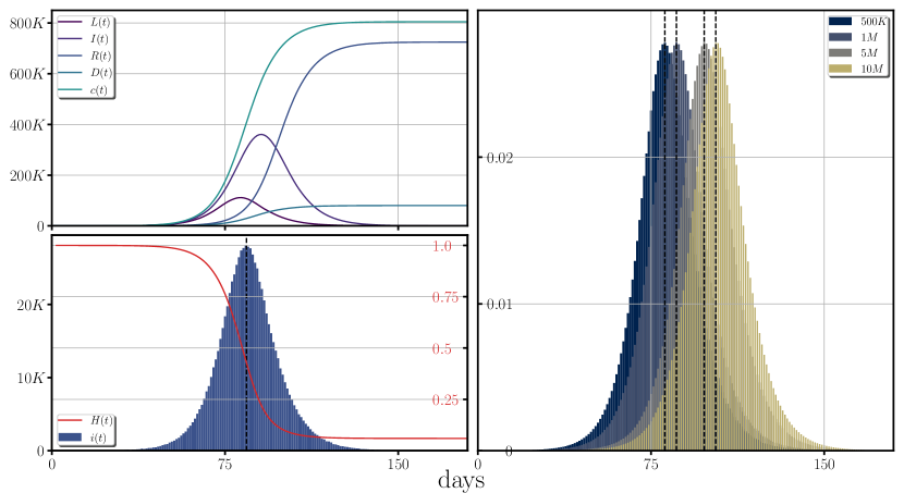
Figure 1: Effects of the weight function representing the herd immunity (i.e. , $W(t)=H(t)$), over the spreading of a disease based on the estimated COVID-19 parameters. At the first column (from left to right), the development of the latent, the infectious, the recovered, the deceased population and the cumulative of the incidence are plotted for a single trajectory. In the next column is plotted the incidence with the form of the weight function representing the heard immunity effect while at the last column the averages over 5000 trajectories of the normalized incidence for different sizes of the population are shown. At the first row, from top to bottom, the simulations are generated when the fluctuations around the mean number of daily infections are generated through a punctual distribution i.e. , no-fluctuations: $\Pi[\varrho_{o}]\rightarrow\{\lambda\}_{i}=\varrho_{o}\delta_{ii}$, while at the second row, the fluctuations are generated from a Gamma distribution with mean $k\theta=\varrho_{o}$ with a standard deviation of $\sigma=1$, i.e. $\Pi[\varrho_{o}]=\mathrm{Gamma}(k=\varrho_{o},\theta=1)\rightarrow\{\lambda\}_{i}$. The epidemiological parameters employed in the figure corresponds to the estimated values of the COVID-19.

From figure 1, one notices that the maximum incidence for a population of one million is obtained of around 3 months after the beginning of the spreading of the disease, reaching at its maximum an amount of roughly 2.5% to 2.7% of the total population. Additionally, if the population is increased in size by one order of magnitude, the maximum is shifted around 20 to 30 days when no contingency measures are implemented in the population. The figure also tell us that for populations from one to ten millions the herd immunity may be reached between 130 to 160 days without confinement.

On the other hand, the effect of non-pharmaceutical strategies implemented in the population to contain the spreading of a disease is another mean to modify the probability of infection. In this regard, one could think that some of the most common or intuitive responses of the population under an epidemiological risk: a confinement responding to the daily experience about the development of the disease, e.g., a confinement depending upon the number of active cases. In other words, when a certain fraction of the population has become symptomatic-infected (or deceased), it becomes more likely that some of the susceptible population has knowledge about infected individuals in their social circles or in the neighboring community, reacting with lockdowns due to the fear of becoming infected. Another possibility is that contingency measures are placed over the population (typically by health authorities) along different stages of the evolution of the disease, attempting (in principal) to find an equilibrium between the public health resources and different economical activities that requires contact among the population. In this case and as we have experienced with the COVID-19 pandemia, all populations have gone through lockdowns and relaxation of the confinements during different stages, which in turn, can be imposed at any time of the epidemiological development by the health authorities.

We use our stochastic model to explore the behavior of the COVID-19 spreading in two different confinement scenarios, a confinement triggered upon the number of infectious population (i.e. the active cases) and confinement regulated by health authorities at different stages of the dispersion of the disease. In the former, we let $C(t)$ to be Gaussian-decaying function of the active cases, triggered once certain part of the population has become infectious-symptomatic or deceased, i.e. :

$$C(t)=1+\left[\exp(-[\gamma\,I(t)/N]^{2}\,)-1\right]\theta(I(t)-I_{o})$$ (9)

where $I(t)$ are the active cases at time $t$, while $I_{o}$ is a threshold telling the amount of active cases at which the confinement function is triggered; $\gamma$ is a decaying-rate parameter describing how strong is the confinement and $N$ is the total population. Figure 2 shows the evolution of the disease for a confinement following a Gaussian decay as described in (9). The left four frames represent $I_{o}=1\%$ and $I_{o}=10\%$ (from top to bottom) and $\gamma=5$ and $\gamma=10$ from the left to the right.

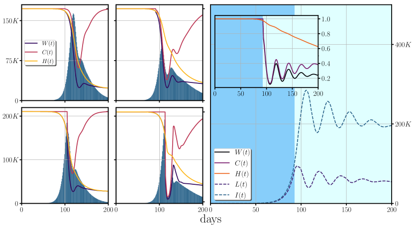
Figure 2: The figure shows the effect of a confinement based on a Gaussian decay as given in (9) for the COVID-19 parameters. At the four left panels, the incidence is shown with the weight function (containing the effects of herd immunity as presented before, and the effects of the confinement), over-imposed on the incidence. The rows from top to bottom show increasing values of $I_{o}$: $I_{o}=5\%$ (top), $I_{o}=10\%$ (bottom), while the columns from left to right show an increasing decaying rate parameter: $\gamma=5$ (left), $\gamma=10$ (right). At the right, the figure shows the effect of a strong and early confinement, $\gamma=50$ and $I_{o}=1\%$, to the latent and the infectious population. All cases corresponds to herd immunity parameters of $\alpha=0.22$ and $i_{o}=0$ and we use a total population of 10 million.

In the figure one can sees that the outcomes of a confinement relying on the number of the infective population depends on how strong and rigorous is the confinement and at what stage of the dispersion of the disease is implemented. The different outcomes goes from a flattening of the epidemic curve, happening when the confinement does not happens abruptly, to revivals in the incidence which become periodic and more pronounced when the confinement is strong and happens at earlier stages of the epidemia. At the right panel we have plotted the latent and the infectious population when $I_{o}=1\%$ (i.e. , the infectious individuals have reached one percent of the population) with an abrupt confinement, $\gamma=50$, from which several revivals can be seen. These revivals can be explained, by looking at the curve of the latent population: in an abrupt confinement, large part of the population remains on the latent condition and when the number of infectious population is reduced, the latent population will tend to break out the confinement measures beginning again with the contagious events. These results exhibit the need to employ correct times and duration of the confinement measures and that abruptly confinements without proper regulatory measures may trigger revivals.

In the context of a confinement based on regulatory measures such as lockdowns, social distancing and restrictions on mobility; they could be implemented at any time of the epidemiological development, it is evident that they will not follow a deterministic behavior (as shown previously). In this regard, in figure 3, we explore the behavior of the spreading of the disease when the probability of infection is manipulated by a piecewise time-dependent $C(t)$ function. In this figure, we show single realizations of the behavior of the incidence and one can sees that if confinement is applied at relatively early stages, then a reduction of the $C(t)$ function below the 25% of its initial value produces a deceleration of the incidence, at 25% the incidence is maintained approximately at a constant rate while anything above the 25% will corresponds to increments in the incidence with stronger accelerations for larger values of the $C(t)$ function. In this regard, figure 3 tell us that it is possible to accelerate, decelerate or keep steady the incidence of a disease with an appropriate manipulation of the weight function. In section IV we use this acquired knowledge to fit the beginning of the spreading of the COVID-19 to real cases happening in Mexico.

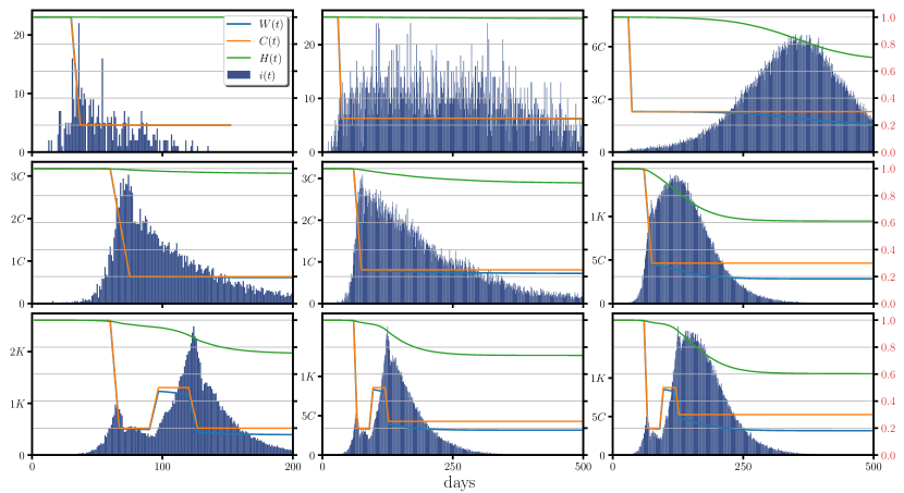
Figure 3: The figure shows the effect of the piecewise confinement (plotted in the embedded small frames) over the incidence, using the COVID-19 parameters in a population of one million. At the first row (from top to bottom), the confinement begins at the day 30 and the decreasing along 7 days the function $C(t)$ from its initial value (one) to a 20% of its initial value (first column), to a 25% of its initial value (second column) and to a 30% from its initial value (third column). At the second row the confinement begins at the day 60 where the function $C(t)$ is decreased from its initial value to a 20% of its initial value (first column), to a 25% of its initial value (second column) and to a 30% from its initial value (third column). Finally at the third row the function $C(t)$ is initially decreased to a 20% of its initial value along a period of 7 days, increased back to a value of a 50% of its initial value along a period of 7 days and finally decreased back again at the day 120 along a period of 7 days to a 20% of its initial value (first column), to a 25% (second column) and to a 30% (third column).

III Interpretation of the weight function

As shown before, the employment of the weight function serves to modulate the mean of the daily infected population and hence it must posses a relation in describing variations of the probability of infection in populations following structured behavior. In this regard, one may ask about the relation between $W(t)$ and the effective reproduction number $\mathcal{R}(t)$, the latter representing the statistical mean of the infections caused by single individuals once the disease has begun to disperse in the population. To answer this question, lets consider first the statistical mean of the number of infected at the time $t_{j}$ due to the $i$-th infectious individual:

$$N_{i}(t_{j})=\sum_{k}[\chi_{i}]_{k}\,p_{k}[\lambda_{i}W(t_{j})]=\lambda_{i}W(t_{j})$$ (10)

where the $[\chi_{i}]_{k}$ represents the possible outcomes of the random variable $\chi_{i}$ of the $i$-th infectious at time $t_{j}$, i.e. , the possible number of infections that the $i-th$ infectious could produce with probability $p_{k}[\lambda_{i}W(t_{j})]$ of the $k$-th event and $\lambda_{i}W(t_{j})$ is the statistical mean of all possible outcomes of the $i$-th contagious individual at time $t_{j}$. In the case where the Poisson parameters $\lambda_{i}$ are also distributed according to a probability distribution $\Pi[\varrho_{o}]$ (see section I), then the average of the total number of infected individuals at a fixed time $t_{j}$ may therefore be given by:

$$\bar{N}(t_{j})=\sum_{i=1}^{I(t_{j})}{N_{i}(t_{j})\over I(t_{j})}=W(t_{j})\,\sum_{i=1}^{I(t_{j})}{\lambda_{i}\over I(t_{j})}.$$ (11)

Let us consider now that in certain given time $t_{j}\geq t^{\prime}$, the number of infectious has become large and representative about the dispersion of the disease in the population, i.e. , the number of infectious can be found homogeneously distributed in the population. This should happen after certain time when all the possible outcomes of the set of the random variables $\lambda_{i}$ are centered around the mean of the distribution $\Pi[\varrho_{o}]$. In other words, for times $t<t^{\prime}$ fluctuations are expected to dominate and as the number of infectious increases, the fluctuations reduce yielding a more localized value of the probability of infection. Therefore, at time $t_{j}>t^{\prime}$ one could approach the number of infected due to the infectious as $\sum_{i=1}^{I(t_{j})}\lambda_{i}/I(t_{j})\sim\varrho_{o}$, yielding us a close relation between the weight function defined earlier and the time-dependent effective reproduction number:

$$\mathcal{R}(t_{j})=\bar{N}(t_{j})t_{I}\sim R_{o}\,W(t_{j})\,.$$ (12)

III.1 Empirical estimation of $\mathcal{R}(t)$.

As seen before, the weight function could be interpreted as a normalization of the time-dependent effective reproduction number, i.e. $W(t)=\mathcal{R}(t)/R_{o}$. In this context, having a self-consistent mechanism that could provide us with an estimation about the evolution of the effective reproduction number based on the real available data, would be desirable. We approximate to this problem by using the information accessible through empirical data, such as the empirical incidence $i_{e}(t)$ and its cumulative $c_{e}(t)$. In our stochastic approximation, the daily synthetic incidence is obtained from a set of random variables following a Poisson distribution; i.e. $i_{s}(t_{j})=\sum_{j=1}^{I(t_{j})}\chi_{i}(t_{j})$, hence the statistical mean of the cumulative of the daily incidence may be written as:

$$\bar{c}_{s}(t_{j})={1\over M}\sum_{l=1}^{M}\sum_{k=1}^{j}\sum_{i=1}^{I_{l}(t_{k})}\chi^{(l)}_{i}(t_{k})$$ (13)

where $M$ represents the total number of trajectories to which the statistical mean is performed. If the number of trajectories is large enough, then the statistical mean will approach the expectation value of the random variables, i.e. , the Poisson parameters associated to the infectious individuals.

By considering the average over the ensemble of the infectious individuals, we can approximate the average of the cumulative as:

$$\bar{c}_{s}(t_{j}) \approx \sum_{k=1}^{j}\sum_{i=1}^{\bar{I}(t_{k})}\lambda_{i}W(t_{k})=\sum_{k=1}^{j}\sum_{i=1}^{\bar{I}(t_{k})}\lambda_{i}\mathcal{R}(t_{k})/R_{o}$$

$$\,,$$ (14)

where in the last line, we have done the replacement of the weight function through the relation obtained earlier in (12). Furthermore, in order to gain convergence, we fix again the Poisson parameters $\lambda_{i}$ to be obtained from a punctual distribution, i.e. $\Pi[\varrho_{o}]\rightarrow\{\lambda\}_{i}=\varrho_{o}\delta_{ii}=R_{o}/t_{I}\,\delta_{ii}$, hence we write for the average of the cumulative:

$$\bar{c}_{s}(t_{j})\approx\sum_{k=1}^{j}\bar{I}(t_{k})\mathcal{R}(t_{k})/t_{I}\,.$$ (15)

Our aim is to give an approximate description about the time dependent reproduction number through empirical quantities; in this regard, we do the replacement of the average synthetic cumulative and the averaged infectious population with their correspondent empirical descriptions; $\bar{c}_{s}(t_{j})\rightarrow c_{e}(t_{j})$ and $\bar{I}(t_{j})\rightarrow I_{e}(t_{j})$. Additionally by expanding the sum in (15) to the first step of propagation and obtaining recurrently the average of the cumulative, is easy to see that the time dependent reproduction number can be obtained as:

$$\mathcal{R}(t_{j})={i_{e}(t_{j})\over I_{e}(t_{j})}t_{I}\,,$$ (16)

while the number of infectious individuals at time $t_{j}$ can be approximated, according the definitions done earlier, as: $I_{e}(t_{j})=\sum_{k=0}^{t_{I}}i_{e}(j-t_{L}-k)$.

IV Development of the COVID-19 in some Mexican states.

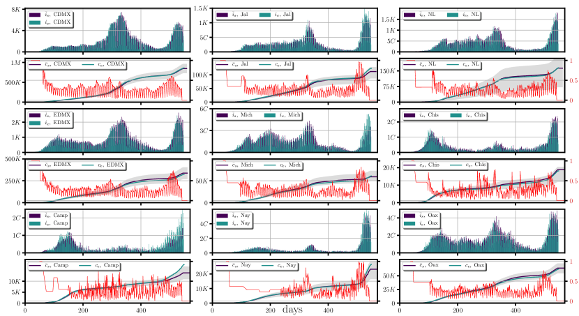
Figure 4: The figure shows a comparison of the incidence and its cumulative, between the synthetic data generated by the stochastic model when averaged over 5000 trajectories to the real scenarios haopening in some Mexican states and Mexico City. The synthetic data was generated by employing the empirical estimation of the effective reproduction number from which the weight function can be obtained: $W(t)=\mathcal{R}(t)/R_{o}$. The figure shows a period of roughly a year and a half of the spreading of the SARS CoV-2 (from February the 18th of 2020 to August the 20th of 2021).

Along the development of the COVID-19 pandemia, we have used the stochastic model to follow the evolution of the spreading of the COVID-19 in certain Mexican states, some of them housing some of the largest Mexican metropolitan areas (i.e. , México City, Estado de México, Jalisco and Nuevo León) and some middle-size populated states. To model the spreading of the COVID-19 in these states, we begin by looking to the empirical incidence and consider an initial infectious estimation by adding the number of the daily new infected population until a the day in which the following days a continuous incidence is sustained (i.e.  there is at least one new infected person reported); afterwards, we perform rough estimations about the form of the weight function following linear decrements (deceleration) or linear increments (acceleration) at certain intervals of time to describe the development of the COVID-19 at the beginning of the spreading, and once the number of infectious individuals has become sufficiently large (in this case we wait until the number of infectious individuals has grown beyond 1000 individuals for the first time), we employ the empirical estimation about the effective reproduction number to describe the evolution of the pandemia in these Mexican states. In these simulations, we only employ the empirical estimations about the effective reproduction number without considering herd immunity effects since under confinement, the pandemia can be considered effectively open in the sense that there is an infinite number of susceptible. The real data has been obtained from the reported cases by the scientific division of the Mexican federal government (CONACyT): https://datos.covid-19.conacyt.mx/. These results are presented in figure 4 for the cumulative of the incidence when averaged over 5000 trajectories. In figure 4 one can notice, in the general, a good agreement between the synthetic data generated from the stochastic model and the real scenarios along the period of dispersion of the disease which was considered of roughly a year and a half. Furthermore, the good agreement indicates that the infections events can be assumed to be time-homogeneously distributed, except for some cases at certain times (e.g. see Campeche around the 450 day) which may suggest the occurrence of anomalous events (possibly superspreading events) for which this assumption may not hold.

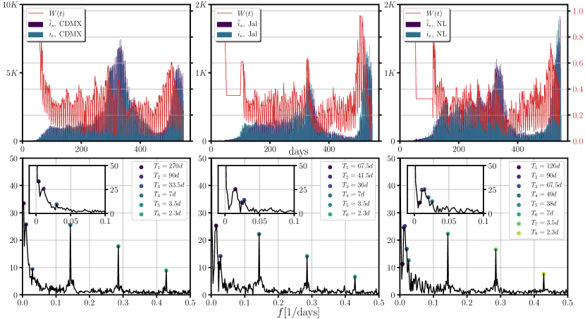
Figure 5: The figure shows the absolute value of the one-sided Fourier transform of the probability of infection derived from the empirical effective reproduction number of Mexico City and the states of Jalisco and Nuevo León. At the first row the empirical and synthetic incidence and the form of the weight function are shown as reference. At the second row the absolute value of the one-sided Fourier transform of the weight function is shown, marking the most relevant frequencies associated to periodic patterns in the effective reproduction number. The figure shows a period of roughly a year and a half of the spreading of the SARS-CoV-2 (from February the 18th of 2020 to August the 20th of 2021).

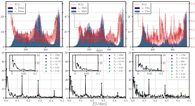
Figure 6: The figure shows the absolute value of the one-sided Fourier transform of the probability of infection derived from the empirical effective reproduction number of the states of Estado de México of Michoacan and Chiapas. At the first row the empirical and synthetic incidence and the form of the weight function are shown as reference. At the second row the absolute value of the one-sided Fourier transform of the weight function is shown, marking the most relevant frequencies associated to periodic patterns in the effective reproduction number. The figure shows a period of roughly a year and a half of the spreading of the SARS-CoV-2 (from February the 18th of 2020 to August the 20th of 2021).

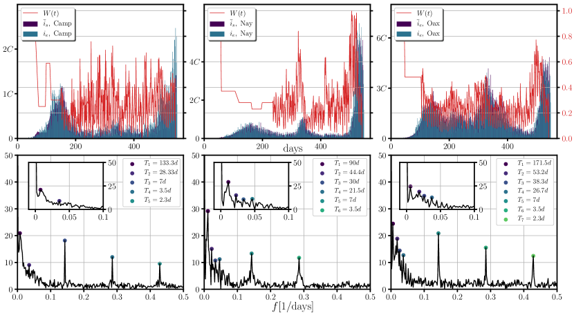
Figure 7: The figure shows the absolute value of the one-sided Fourier transform of the probability of infection derived from the empirical effective reproduction number of the states of Campeche of Nayarit and Oaxaca. At the first row the empirical and synthetic incidence and the form of the weight function are shown as reference. At the second row the absolute value of the one-sided Fourier transform of the weight function is shown, marking the most relevant frequencies associated to periodic patterns in the effective reproduction number. The figure shows a period of roughly a year and a half of the spreading of the SARS-CoV-2 (from February the 18th of 2020 to August the 20th of 2021).

Once we have confirmation about the good agreement of the model, we turn our attention to the empirical weight function (i.e.  the normalized effective reproduction number) and look for periodic patterns in the daily mean of infections. The period of these patterns can be obtained by performing the Fourier transform of the weight function where the peaks appearing in the spectrum of the weight function will corresponds to the frequencies associated to these periods and could provide us with information about the implementation of confinement, testing, mobility, or even emergent periodic behavior encoded in the probability of infection, during the development of the COVID-19.

In figures 5 to 7 we present the absolute value of the one-sided Fourier transform of the weight function (second row) of each of the Mexican states analyzed before (first row). In the figure we identify three set of frequencies whose corresponding periods lies on different time scales which we believe are related to the weekly agenda, confinements and also to larger patterns such as pandemic waves or even the emergence of seasonality. We identify a first set belonging to periods within a week for which in almost all the cases (with the exception of Nayarit, which in addition, it has been one of the states with the smaller incidence rate before the third pandemic wave) three peaks are present exactly at the same periods i.e.  at $7$ days, $3.5$ days and $2.3$ days which may confirm a global (not local) behavior and we believe these are related to the weekly agenda concerning the periodicity of the testing and the capture of the readouts. A second time scale lies on the range from one two six months which we believe are connected to pandemic waves or periods of confinement, de-confinement and holiday seasons. For this time scale one observes periods that are shared by certain states (see e.g.  the periods of 90 days appearing in México City, Estado the México, Nuevo León and Nayarit, or the state of Jalisco and Michoacan which share periods of 67.5 days and 41.4 days, the latter also shared by Estado de México) and additional periods which are unique of the particular cases. The shared periods could be explained due to the closeness of certain states (such is the case of México City and Estado the México or Jalisco and Michoacan) or due to the connections of large populated regions such as Nuevo León with México city and Estado de México. The larger time scale is represented by the first peak appearing in México City and Estado de México which is not surprising they shared this peak since they large neighboring metropolitan areas. This peak corresponds to a periodic pattern emerging at $T_{1}=297$ days, suggesting which may be related to pandemic waves or even the emergence of a seasonal behavior of the COVID-19. This time scale is only present in these states and it may be consequence of the amount of the population that has become infected (notice that in Mexico City the amount of infected population is roughly one order of magnitude greater than the states of Jalisco and Nuevo León), and the large degree of urbanization of this region.

V Conclusion

In this paper we have derived an stochastic compartmental epidemiological model constructed from first principles which consist on a randomization about the number of the new infected population caused daily and by assuming that the infectious events follow a Poisson process. We have shown that under this assumption, one can reconstruct and simulate emergent phenomena such as herd immunity or certain confinement scenarios, by introducing an additional time-dependent function (the weight function) which can be represented as a normalization of the time-dependent effective reproduction number which additionally has helped us to modulate the mean of the daily new infections, (and hence the probability of infection) along the evolution of the disease. Moreover, we have derived an empirical estimation about the weight function which has serve us to incorporate self-consistency into the model. Along this paper, we have focused on the epidemiological parameters corresponding to the COVID 19 disease and through the employment of the weight function, the model is capable to introduce and study some conceptual behaviors such as herd immunity or certain idealized confinement scenarios. In the former we have employed an inverse-like logistic function of the fraction of the total infected population, which for the COVID-19 epidemiological parameters and without any confinement measures, we have found that the peak of the incidence scales by 20 to 30 days when the total population is increased by one order of magnitude while independently of the population sizes, the maximum incidence reaches a reaching 2.5% to 2.7% of the total population; in the latter, we have explored the reaction of the dispersion of the disease when the population reacts to the infectious population (representing an intuitive reaction of the population under an epidemiological emergence), finding revivals in the incidence (infective waves) if confinement is abrupt and happens at earlier stages in the dispersion of the disease, and a flattening of the epidemic curve on the contrary situation. Furthermore, we have simulated the effects on the incidence when the weight function is described through a piecewise function finding accelerations in the incidence when the weight function takes values above 25% of its initial value, a steady behavior for a 25% of its initial value and deceleration in the incidence when the weight function take values below the 25% of its initial value.

We have employed our stochastic model model together with the definition of the empirical weight function, to simulate the dispersion of the COVID-19 in some Mexican states, some of them housing the major metropolitan areas in Mexico and finding a very good agreement to the real scenarios implying that the infectious events in México could be interpreted as homogeneously distributed events.

Finally, we have applied the one-sided Fourier transform to the empirical description of the weight function with the intention to look at periodic patterns emerging in the mean of the daily infection which may give us insights about the evolution of the pandemia in México. In this regard, we have found three different set of frequencies corresponding to different time-scales which we identify to a weekly agenda about the capture of the readouts of the testings, confinement and also larger patterns which may be related to pandemic waves or even seasonality.

The standard SIR model limit

In the context of the standard SIR model, the susceptible population $S$ has to be considered corresponding to the part of the population which can be infected. In this regard, its number is constantly reducing due to the contagious events, therefore, according to the random scenario we have proposed, at the time $t_{j+1}$ the number of susceptible can be described as:

$$S(t_{j+1})=S(t_{j})-\sum_{i=1}^{I(t_{j})}\chi_{i}(t_{j})\,.$$ (17)

with the last term accounting for the part of the susceptible population skiping out from this conditon into the latent condition.

From our random model, the standard SIR model can be derived by considering that at any fixed time $t_{j}$, any infectious individual infects the same amount of susceptible. This assumptions can be considered valid, (althouhg unrealistic somehow), when the population is homogenously distributed along the infection area at all time, i.e. , there are no clusters of individuals in the population and the reorganization of the susceptible popultion every time step is homogeneously distributed in space. In this regard, the SIR model limit relies on the assumptions that the distribution of the individuals of the population is independent of the antropological characteristics of the society.

Following within this idea, we do the replacement of the new daily infected population by each infectious individual by a constant ammount $S_{o}(t_{j})$; the total amount of new infected population at the time $t_{j}$ will yield:

$$\sum_{i=1}^{I(t_{j})}\chi_{i}(t_{j}) = \sum_{i=1}^{I(t_{j})}S_{o}(t_{j})$$ (18)

$$= S_{o}(t_{j})\,I(t_{j})\,.$$

Moreover, under this assumption, the number of the daily new infected population is scalable in time, hence the population of susceptible can be thought as reservoir of individuals of infinite size such that the epidemic events will not alter the homogenity of the distribution and one can connect the number of susceptible per unit time $\delta_{t}=t_{j}-t_{j-1}$, to the total number of susceptible in the long time limit, i.e.   $S_{o}(t_{j})/\delta_{t}=S(t_{j})/n\delta_{t}$. Finally, by redefining the number of the infected population as $L+I\rightarrow I$ and by considering the limit of infinitesimal time steps (which will be valid only for very large population sizes) then, one can write now the set of deterministic equations of the SIR model about the evolution of the disease as:

$$\dot{S}(t) = -\beta\,S(t)\,I(t),$$ (19)

$$\dot{I}(t) = \beta\,S(t)\,I(t)-\kappa_{R}\,I(t)\,,$$ (20)

$$\dot{R}(t) = \kappa_{R}\,I(t)\,.$$ (21)

where contact rate defined as the average number of contacts per individuals per time will be given by $\beta=\lim_{\delta_{t}\rightarrow 0}(n\delta t)^{-1}$ while the recovery rate will fulfill: $\kappa_{R}=\lim_{\delta_{t}\rightarrow 0}(r\delta_{t})^{-1}$, with $r$ being a recovery-time scale factor, i.e. $t_{R}=r\delta_{t}$. Clearly, for both rates as $\delta_{t}\rightarrow 0$ the quantities $n\delta t$ and $r\delta t$ remain finite.

Additional information

Accession codes:https://github.com/RenatoSalArrDu/StochasticSLIRD

References

- World Health Organisation (2021a) World Health Organisation, (2021a), https://covid19.who.int/, Last accessed on 2021-09-09.
- Shankar et al. (2021) S. Shankar, S. S. Mohakuda, A. Kumar, P. Nazneen, A. K. Yadav, K. Chatterjee, and K. Chatterjee, Medical journal, Armed Forces India 77, S385—S392 (2021).
- Weiss (2013) H. Weiss, Materials Matemàtics 3, 17 (2013).
- Read et al. (2021) J. M. Read, J. R. E. Bridgen, D. A. T. Cummings, A. Ho, and C. P. Jewell, Philosophical Transactions of the Royal Society B: Biological Sciences 376, 20200265 (2021), https://royalsocietypublishing.org/doi/pdf/10.1098/rstb.2020.0265 .
- Cao et al. (2020) Z. Cao, Q. Zhang, X. Lu, D. Pfeiffer, Z. Jia, H. Song, and D. D. Zeng, medRxiv (2020), 10.1101/2020.01.27.20018952, https://www.medrxiv.org/content/early/2020/01/29/2020.01.27.20018952.full.pdf .
- Tang et al. (2020) B. Tang, X. Wang, Q. Li, N. L. Bragazzi, S. Tang, Y. Xiao, and J. Wu, Journal of clinical medicine 9, 462 (2020), 32046137[pmid].
- Danon et al. (2021) L. Danon, E. Brooks-Pollock, M. Bailey, and M. Keeling, Philosophical Transactions of the Royal Society B: Biological Sciences 376, 20200272 (2021), https://royalsocietypublishing.org/doi/pdf/10.1098/rstb.2020.0272 .
- Wu et al. (2020) J. T. Wu, K. Leung, and G. M. Leung, The Lancet 395, 689 (2020).
- Riou and Althaus (2020) J. Riou and C. L. Althaus, Euro surveillance : bulletin Europeen sur les maladies transmissibles = European communicable disease bulletin 25, 2000058 (2020).
- Sanche et al. (2020) S. Sanche, Y. T. Lin, C. Xu, E. Romero-Severson, N. Hengartner, and R. Ke, Emerging infectious diseases 26, 1470—1477 (2020).
- Chinazzi et al. (2020) M. Chinazzi, J. T. Davis, M. Ajelli, C. Gioannini, M. Litvinova, S. Merler, A. Pastore y Piontti, K. Mu, L. Rossi, K. Sun, C. Viboud, X. Xiong, H. Yu, M. E. Halloran, I. M. Longini, and A. Vespignani, Science 368, 395 (2020), https://science.sciencemag.org/content/368/6489/395.full.pdf .
- Wong et al. (2020) G. N. Wong, Z. J. Weiner, A. V. Tkachenko, A. Elbanna, S. Maslov, and N. Goldenfeld, Phys. Rev. X 10, 041033 (2020).
- Chang et al. (2021) S. Chang, E. Pierson, P. W. Koh, J. Gerardin, B. Redbird, D. Grusky, and J. Leskovec, Nature 589, 82 (2021).
- Borremans et al. (2017) B. Borremans, J. Reijniers, N. Hens, and H. Leirs, Royal Society Open Science 4, 171308 (2017), https://royalsocietypublishing.org/doi/pdf/10.1098/rsos.171308 .
- Fukś et al. (2006) H. Fukś, A. T. Lawniczak, and R. Duchesne, The European Physical Journal B - Condensed Matter and Complex Systems 50, 209 (2006).
- World Health Organisation (2021b) World Health Organisation, (2021b), https://www.who.int/emergencies/diseases/novel-coronavirus-2019/technical-guidance/maintaining-essential-health-services-and-systems, Last accessed on 2021-09-09.
- Gilbert et al. (2020) M. Gilbert, G. Pullano, F. Pinotti, E. Valdano, C. Poletto, P.-Y. Boëlle, E. D’Ortenzio, Y. Yazdanpanah, S. P. Eholie, M. Altmann, B. Gutierrez, M. U. G. Kraemer, and V. Colizza, The Lancet 395, 871 (2020).
- Pullano et al. (2020) G. Pullano, F. Pinotti, E. Valdano, P.-Y. Boëlle, C. Poletto, and V. Colizza, Euro surveillance : bulletin Europeen sur les maladies transmissibles = European communicable disease bulletin 25, 2000057 (2020), 32019667[pmid].
- Balcan et al. (2009) D. Balcan, V. Colizza, B. Gonçalves, H. Hu, J. J. Ramasco, and A. Vespignani, Proceedings of the National Academy of Sciences 106, 21484 (2009), https://www.pnas.org/content/106/51/21484.full.pdf .
- Danon et al. (2009) L. Danon, T. House, and M. J. Keeling, Epidemics 1, 250 (2009).
- Dordević et al. (2021) J. Dordević, I. Papić, and N. Šuvak, Chaos, Solitons and Fractals 148, 110991 (2021).
- Adak et al. (2021) D. Adak, A. Majumder, and N. Bairagi, Chaos, Solitons and Fractals 142, 110381 (2021).
- Engbert et al. (2020) R. Engbert, M. M. Rabe, R. Kliegl, and S. Reich, Bulletin of Mathematical Biology 83, 1 (2020).
- Hazarie et al. (2021) S. Hazarie, D. Soriano-Paños, A. Arenas, J. Gómez-Gardeñes, and G. Ghoshal, Communications Physics 4, 191 (2021).
- Li et al. (2020) Q. Li, X. Guan, P. Wu, X. Wang, L. Zhou, Y. Tong, R. Ren, K. S. Leung, E. H. Lau, J. Y. Wong, X. Xing, N. Xiang, Y. Wu, C. Li, Q. Chen, D. Li, T. Liu, J. Zhao, M. Liu, W. Tu, C. Chen, L. Jin, R. Yang, Q. Wang, S. Zhou, R. Wang, H. Liu, Y. Luo, Y. Liu, G. Shao, H. Li, Z. Tao, Y. Yang, Z. Deng, B. Liu, Z. Ma, Y. Zhang, G. Shi, T. T. Lam, J. T. Wu, G. F. Gao, B. J. Cowling, B. Yang, G. M. Leung, and Z. Feng, New England Journal of Medicine 382, 1199 (2020), pMID: 31995857, https://doi.org/10.1056/NEJMoa2001316 .
- Guan et al. (2020) W.-j. Guan, Z.-y. Ni, Y. Hu, W.-h. Liang, C.-q. Ou, J.-x. He, L. Liu, H. Shan, C.-l. Lei, D. S. Hui, B. Du, L.-j. Li, G. Zeng, K.-Y. Yuen, R.-c. Chen, C.-l. Tang, T. Wang, P.-y. Chen, J. Xiang, S.-y. Li, J.-l. Wang, Z.-j. Liang, Y.-x. Peng, L. Wei, Y. Liu, Y.-h. Hu, P. Peng, J.-m. Wang, J.-y. Liu, Z. Chen, G. Li, Z.-j. Zheng, S.-q. Qiu, J. Luo, C.-j. Ye, S.-y. Zhu, and N.-s. Zhong, New England Journal of Medicine 382, 1708 (2020), https://doi.org/10.1056/NEJMoa2002032 .
- Backer et al. (2020) J. A. Backer, D. Klinkenberg, and J. Wallinga, Euro surveillance : bulletin Europeen sur les maladies transmissibles = European communicable disease bulletin 25, 2000062 (2020), 32046819[pmid].
- Tindale et al. (2020) L. C. Tindale, J. E. Stockdale, M. Coombe, E. S. Garlock, W. Y. V. Lau, M. Saraswat, L. Zhang, D. Chen, J. Wallinga, and C. Colijn, eLife 9, e57149 (2020), 32568070[pmid].
- John and Samuel (2000) T. J. John and R. Samuel, Eur J Epidemiol 16, 601 (2000).
- Rashid et al. (2012) H. Rashid, G. Khandaker, and R. Booy, Current Opinion in Infectious Diseases 25 (2012).