Improved Input Reprogramming for GAN Conditioning

Abstract

We study the GAN conditioning problem, whose goal is to convert a pretrained unconditional GAN into a conditional GAN using labeled data. We first identify and analyze three approaches to this problem – conditional GAN training from scratch, fine-tuning, and input reprogramming. Our analysis reveals that when the amount of labeled data is small, input reprogramming performs the best. Motivated by real-world scenarios with scarce labeled data, we focus on the input reprogramming approach and carefully analyze the existing algorithm. After identifying a few critical issues of the previous input reprogramming approach, we propose a new algorithm called InRep+. Our algorithm InRep+ addresses the existing issues with the novel uses of invertible neural networks and Positive-Unlabeled (PU) learning. Via extensive experiments, we show that InRep+ outperforms all existing methods, particularly when label information is scarce, noisy, and/or imbalanced. For instance, for the task of conditioning a CIFAR10 GAN with $1\%$ labeled data, InRep+ achieves an average Intra-FID of $76.24$, whereas the second-best method achieves $114.51$.

1 Introduction

Generative Adversarial Networks (GANs) [1] have introduced an effective paradigm for modeling complex high dimensional distributions, such as natural images [2, 3, 4, 5, 6, 7, 8], videos [9, 10], audios [7, 11] and texts [7, 8, 12, 13]. With recent advancements in the design of well-behaved objectives [14], regularization techniques [15], and scalable training for large models [16], GANs have achieved impressively realistic data generation.

Conditioning has become an essential research topic of GANs. While earlier works focus on unconditional GANs (UGANs), which sample data from unconditional data distributions, conditional GANs (CGANs) have recently gained a more significant deal of attention thanks to their ability to generate high-quality samples from class-conditional data distributions [2, 17, 18]. CGANs provide a broader range of applications in conditional image generation [17], text-to-image generation [19], image-to-image translation [5], and text-to-speech synthesis [20, 21].

In this work, we define a new problem, which we dub GAN conditioning, whose goal is to learn a CGAN given (a) a pretrained UGAN and (b) labeled data. The pretrained UGAN is given in the form of an unconditional generator. Also, we assume that the classes of the labeled data are exclusive to each other, that is, the true class-conditional distributions are separable. Fig. 1 illustrates the problem setting with a two-class MNIST dataset. The first input, shown on the top left of the figure, is an unconditional generator $G$, which is trained on a mixed dataset of classes $0$ and $1$. The second input, shown on the bottom left of the figure, is a labeled dataset. In this example, the goal of GAN conditioning algorithms is to learn a two-class conditional generator $G^{\prime}$ from these two inputs, as shown on the right of Fig. 1.

Formally, given an unconditional generator $G$ trained with unlabeled data drawn from $p_{\text{data}}({\bm{x}})$ and a conditional dataset ${\mathbb{D}}$ where ${\mathbb{D}}=\bigcup_{y\in{\mathbb{Y}}}{\mathbb{D}}(y)$ with ${\mathbb{Y}}$ being the label set and ${\mathbb{D}}(y)$ being drawn from $p_{\text{data}}({\bm{x}}|y)$, GAN conditioning algorithms learn a conditional generator $G^{\prime}$ that generates $y$-conditional samples given label $y\in\mathbb{Y}$. The formulation of the GAN conditioning problem is motivated by several practical scenarios. The first scenario is pipelined training. For illustration, we consider a learner who wants to learn a text-to-speech algorithm using CGANs. While labeled data is being collected (that is, text-speech pairs), the learner can start making use of a large amount of unlabeled data, which is publicly available, by pretraining a UGAN. Once labeled data is collected, the learner can then use both the pretrained UGAN and the labeled data to learn a CGAN more efficiently. This approach enables a pipelined training process to utilize better the long waiting time required for labeling. Secondly, GAN conditioning is helpful in a specific online or streaming learning setting, where the first part of the data stream is unlabeled, and the remaining data stream is labeled. Assuming that it is impossible to store the streamed data due to storage constraints, one must learn something in an online fashion when samples are available and then discard them right away. Now consider the setting where the final goal is to train a CGAN. One may discard the unlabeled part of the data stream and train a CGAN on the labeled part, but this will be strictly suboptimal. One plausible approach to this problem is to train a UGAN on the unlabeled part of the stream and then apply GAN conditioning with the labeled part of the stream. The third scenario is in transferring knowledge from models pretrained on private data. In many cases, pretrained UGAN models are publicly available while the training data is not, primarily because of privacy. An efficient algorithm for GAN conditioning can be used to transfer knowledge from such pretrained UGANs when training a CGAN.

Existing approaches to GAN conditioning can be categorized into three classes. The first and most straightforward approach is discarding UGAN and applying the CGAN training algorithms [2, 17, 18] on the labeled data. However, training a CGAN from scratch not only faces performance degradation if the labeled data is scarce or noisy [22, 23, 24] but also incurs enormous resources in terms of time, computation and memory. The second approach is fine-tuning the UGAN into a CGAN. While fine-tuning GANs [25, 26] provides a more efficient solution than the full CGAN training, this method may suffer from the catastrophic forgetting phenomenon [27].

Recent studies [28, 29] propose a new approach to GAN conditioning, called input reprogramming. They show that this approach can achieve promising performances with remarkable computing savings. However, their frameworks [28, 29] are designed to handle only one-class datasets. Therefore, to handle multi-class datasets, one must repeatedly apply the algorithm to each class, incurring huge memory when the number of classes is large. Furthermore, the full CGAN training methods still achieve better conditioning performances than the existing input reprogramming methods when the labeled data is sufficiently large. Also, it remains unclear how the performance of input reprogramming-based approaches compares with that of the other approaches as the quality and amount of labeled data vary.

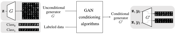
Figure 1: GAN conditioning setting (illustrated with two-class MNIST). GAN conditioning algorithms convert an unconditional generator $G$ (top left) into a conditional generator $G^{\prime}$ (right) using a labeled dataset (bottom left). On the two-class MNIST data, unconditional generator $G$ uniformly generates images of $0$s or $1$s from random noise vector ${\mathbf{z}}$. The labeled data contains class-conditional images with labels $0$ and $1$. The output of the GAN conditioning algorithm is the conditional generator $G^{\prime}$ that generates samples of class $y$ from random noise ${\mathbf{z}}$ and the provided class label $y$ in $\{y_{0}=0,y_{1}=1\}$.

In this work, we thoroughly study the possibility of the input reprogramming framework for GAN conditioning. We analyze the limitations of the existing algorithms and propose InRep+ as an improved input reprogramming framework to fully address the problems identified. Shown in Fig. 2 is the design of our framework. InRep+ learns a conditional network $M$, called modifier, that transforms a random noise ${\bm{z}}$ into a $y$-conditional noise ${\bm{z}}_{y}$ from which the unconditional generator $G$ generates a $y$-conditional sample. We learn the modifier network via adversarial training. InRep+ adopts the invertible architecture [30, 31, 32] for the modifier to prevent the class-overlapping in the latent space. We address the large memory issue by sharing the learnable networks between classes. Also, we make use of Positive-Unlabeled learning (PU-learning) [33] for the discriminator loss to overcome the training instability.

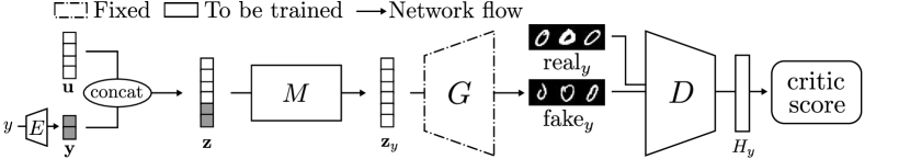
Figure 2: Modular design of InRep+ (Improved Input Reprogramming) framework. Given a fixed unconditional generator $G$, InRep+ learns a modifier network $M$ and conditional discriminator networks $D_{y}$, $y\in{\mathbb{Y}}$. Each $D_{y}$ is built on a weight-sharing network $D$ followed by a class-specific linear head $H_{y}$, i.e. $D_{y}=H_{y}\circ D$. We embed each label $y$ into a vector ${\mathbf{y}}$ with the embedding module $E$, then concatenate ${\mathbf{y}}$ to a random noise vector ${\mathbf{u}}$ to get vector ${\mathbf{z}}$. The modifier $M$ converts ${\mathbf{z}}$ into a $y$-conditional noise ${\mathbf{z}}_{y}$ so that $G({\mathbf{z}}_{y})$ is a sample of class $y$ (a $0$-image of $\text{fake}_{y}$ in the illustration). We train our networks using GAN training.

Via theoretical analysis, we show that InRep+ is optimal with the guaranteed convergence given the optimal UGAN. Our extensive empirical study shows that InRep+ can efficiently learn high-quality samples that are correctly conditioned, achieving state-of-the-art performances regarding various quantitative measures. In particular, InRep+ significantly outperforms other approaches on various datasets when the amount of labeled data is as small as $1$% or $10$% of the amount of unlabeled data used for training UGAN. We also demonstrate the robustness of InRep+ against label-noisy and class-imbalanced labeled data.

The rest of our paper is organized as follows. We first review the existing approaches to GAN conditioning in Sec. 2. In Sec. 3, we analyze the existing input reprogramming framework for GAN conditioning and propose our new algorithm InRep+. In Sec. 4, we empirically evaluate InRep+ and other GAN conditioning methods in various training settings. Finally, Sec. 5 provides further discussions on the limitation of our proposed approach as well as the applicability of InRep+ to other generative models and prompt tuning. We conclude our paper in Sec. 6.

Notation

We follow the notations and symbols in the standard GAN literature [1, 34]. That is, $a,{\bm{a}},{\textnormal{a}},{\mathbf{a}},{\mathbb{A}}$ denote a scalar, vector, random scalar variable, random vector variable, and set; ${\bm{x}},y,{\bm{z}}$ denote a feature vector, label, and input noise vector, respectively.

2 Preliminaries on GAN conditioning

We review three existing approaches to GAN conditioning: (1) discarding UGAN and training a CGAN from scratch, (2) fine-tuning [25, 26], and (3) input reprogramming [28, 29]. In particular, we analyze their advantages, drawbacks, and requirements for GAN conditioning. Sec. 2.4 summarizes our high-level comparison of their performances in various training settings of labeled data and computing resources.

2.1 Learning CGAN without using UGAN

One can discard the given UGAN and apply the existing CGAN training algorithms on the labeled dataset to learn a CGAN. This approach is the most straightforward approach for GAN conditioning.

We can group CGAN training algorithms by strategies of incorporating label information into the training procedure. The first strategy is to concatenate or embed labels to inputs [17, 35] or to middle-layer features [19, 36]. The second strategy, which generally achieves better performance, is to design the objective function to incorporate conditional information. For instance, ACGAN [18] adds a classification loss term to the original discriminator objective via an auxiliary classifier. Recent algorithms adopt label projection in the discriminator [2] by linearly projecting the embedding of the label vector into the feature vector. Based on the projection-based strategy, ContraGAN [4] further utilizes the data-data relation between samples to achieve better quality and diversity in data generation.

Directly applying such CGAN algorithms for GAN conditioning may achieve state-of-the-art conditioning performances if sufficient labeled data and computing resources are available. However, this is not always the case in practice, and the approach also has some other drawbacks. The scarcity of labeled data in practice can severely degrade the performance of CGAN algorithms [24]. Though multiple techniques [3, 37] were proposed to overcome this scarcity issue, mainly by using data augmentation to increase labeled data, these techniques are orthogonal to our work, and we consider only the standard algorithms. Furthermore, training CGAN from scratch is notoriously challenging and expensive. Researchers observed various factors that make CGAN training difficult, such as instability [22, 23], mode collapse [38, 23], or mode inventing [38]. Also, the training usually entails enormous resources in terms of time, computation, and memory, which are not available for some settings, such as mobile or edge computing. For instance, training BigGAN [39] takes approximately 15 days on a node with $8$x NVIDIA Tesla V100/32GB GPUs [16].

Additionally, some CGAN training algorithms have inductive biases, which may cause failures in learning the true distributions. The following lemmas investigate several failure scenarios of the two most popular conditioning strategies – ACGAN [18] and ProjGAN [2], and we defer the formal statements and proofs to Appendix A.1.

Failures of auxiliary classifier conditioning strategy

The discriminator and generator of ACGAN learn to maximize $\lambda L_{C}+L_{S}$ and $\lambda L_{C}-L_{S}$, respectively. Here, $L_{S}$ models the log-likelihood of samples belonging to the real data, $L_{C}$ models the log-likelihood of samples belonging to the correct classes, and $\lambda$ is a hyperparameter balancing the two terms. In this game, $G$ might be able to maximize $\lambda L_{C}-L_{S}$ by simply learning a biased distribution (increased $L_{C}$) at the cost of compromised generation quality (increased $L_{S}$). Our following lemmas show that ACGAN indeed suffers from this phenomenon, for both non-separable datasets (Lemma 1) and separable datasets (Lemma 2). We also note that the failure in non-separable datasets has been previously studied in [40], while the one with separable datasets has not been shown before in the literature.

Lemma 1 (ACGAN provably fails on a non-separable dataset).

Suppose that the data follows a Gaussian mixture distribution with a known location but unknown variance, and the generator is a Gaussian mixture model parameterized by its variance. Assume the perfect discriminator. For some values of $\lambda$, the generator’s loss function has strictly suboptimal local minima, thus gradient descent-based training algorithms fail to find the global optimum.

Lemma 2 (ACGAN provably fails on a separable dataset).

Suppose that the data are vertically uniform in $2$D space: conditioned on $y\in\{\pm 1\}$, ${\mathbf{x}}=(d\cdot{\textnormal{y}},{\textnormal{u}})$ with some $d>0$ and u is uniformly distributed in $[-1,1]$. An auxiliary classifier is a linear classifier, passing the origin. Assume the perfect discriminator. For some single-parameter generators, gradient descent-based training algorithms converge to strictly suboptimal local minima.

Failures of projection-based conditioning strategy

The objective function of a projection-based discriminator [2] measures the orthogonality between the data feature vector and its class-embedding vector in the form of an inner product. Thus, even when the generator learns the correct conditional distributions, it may continue evolving to further orthogonalize the inner product term if the class embedding matrix is not well-chosen. This behavior of the generator can result in learning an inexact conditional distribution, illustrated in the following lemma.

Lemma 3 (ProjGAN provably fails on a two-class dataset).

Consider a simple projection-based CGAN with two equiprobable classes. With some particular parameterizations of the discriminator, there exist bad class-embedding vectors that encourage the generator to deviate from the exact conditional distributions.

2.2 Fine-tuning UGAN into CGAN

The fine-tuning approach aims to adjust the provided unconditional generator into a conditional generator using the labeled data. Previous works [25, 26] studied fine-tuning GANs for knowledge transfer in GANs. We can further adapt these approaches for GAN conditioning. TransferGAN [25] introduces a new framework for transferring GANs between different datasets. They propose to fine-tune both the pretrained generator and discriminator networks. MineGAN [26] later suggests fixing the generator and training an extra network (called the miner) to optimize the latent noises for the target dataset before fine-tuning all networks. We note that in the GAN conditioning setting, the pretrained discriminator is not available. Furthermore, to be applicable for GAN conditioning, TransferGAN and MineGAN frameworks may require further modifications of unconditional generators’ architecture to incorporate the conditional information. Unlike fine-tuning approaches, our method freezes the $G$ and does not modify its architecture or use the pretrained unconditional discriminator.

Compared to the full CGAN training, fine-tuning approaches usually require much less training time and amount of labeled data while still achieving competitive performance. However, it is not clear how one will modify the architecture of the unconditional generator for a conditional one. Also, fine-tuning techniques are known to suffer from catastrophic forgetting [27], which may severely affect the quality of generated samples from well-trained unconditional generators.

2.3 Input reprogramming

The overarching idea of input reprogramming is to keep the well-trained UGAN intact and add a controller module to the input end for controlling the generation. In particular, this approach aims to repurpose the unconditional generator into a conditional generator by only learning the class-conditional latent vectors.

Input reprogramming can be considered as neural reprogramming [41] applied to generative models. Neural reprogramming (or adversarial reprogramming) [41] has been proposed to repurpose pretrained classifiers for alternative classification tasks by just preprocessing their inputs and outputs. Recent works extend neural reprogramming to different settings and applications, such as the discrete input space for text classification tasks [42] and the black-box setting for transfer learning [43]. More interestingly, it has been shown that large-scale pretrained transformer models can also be efficiently repurposed for various downstream tasks, with most of the pretrained parameters being frozen [44]. On the theory side, the recent work [45] shows that the risk of a reprogrammed classifier can be upper bounded by the sum of the source model’s population risk and the alignment loss between the source and the target tasks.

Input reprogramming has been previously studied under various generative models and learning settings. Early works attempt to reprogram the latent space of GAN with pretrained classifiers [46] or the latent space of variational autoencoder (VAE) [28] via CGAN training. Flow-based models can also be repurposed for the target attributes via posterior matching [47]. The recent work [48] proposes to formulate the conditional distribution as an energy-based model and train a classifier on the latent space to control conditional samples of unconditional generators. However, their training requires manually labeling latent samples and a new sampling method based on ordinary differential equation solvers. We also notice that our work has a different assumption on the input as the only source of supervision in GAN conditioning comes from the labeled data. Recently, GAN-Reprogram [29] via CGAN training obtains high-quality conditional samples with significant reductions of computing and label complexity. GAN-Reprogram is our closest input reprogramming algorithm for GAN conditioning.

For the advantages, input reprogramming methods obtain the competitive performances in the conditional generation on various image datasets, even with limited labeled data. Input reprogramming significantly saves computing and memory resources as the approach requires only an extra lightweight network for each inference. However, the existing algorithm of input reprogramming for GAN conditioning, GAN-Reprogram [29], still underperforms the latest CGAN algorithms on complex datasets. In addition, it focuses solely on one condition per time, leading to the huge memory given a large number of classes, which will be detailed in the next section.

Our proposed method (InRep+) makes significant improvements on GAN-Reprogram. We improve the conditioning performance with invertible networks and a new loss based on the Positive Unlabeled learning approach. We reduce the memory footprints by sharing weights between class-conditional networks. Our study will exhibit that input reprogramming can generate sharper distribution even with small amounts of supervision, leading to consistent performance improvements. We also explore the robustness of input reprogramming in the setting of imbalanced supervision and noisy supervision, which have not been discussed in the literature yet.

2.4 Summary of comparison

Table 1: A high-level comparison of GAN conditioning approaches under various settings (✓= poor, ✓✓= okay, ✓✓✓= good). When labeled data and computing resources are both sufficient, we can discard the unconditional generator and directly apply CGAN algorithms on the labeled data to achieve the best performances. When the amount of labeled data is large, but resources are restricted, the fine-tuning approach becomes a good candidate for GAN conditioning. However, when both labeled data and resources are restricted, input reprogramming becomes the best solution for GAN conditioning. Our method InRep+ improves both the conditioning performance and the memory scalability of the existing input reprogramming algorithm (GAN-Reprogram).

Setting	Learning CGAN w/o UGAN	Fine-tuning	Input reprogramming
			GAN-Reprogram	InRep+ (ours)
Large labeled data	✓✓✓	✓✓	✓	✓✓
Limited labeled data	✓	✓✓	✓✓	✓✓✓
Limited computation	✓	✓✓	✓✓✓	✓✓✓

Table 1 summarizes our high-level comparison of the analyzed approaches. For input reprogramming, we distinguish between the existing approach GAN-Reprogram and our proposed InRep+. First, when both the labeled data and computation resources are sufficient, using CGAN algorithms without UGAN probably achieves the best conditioning performance, followed by the fine-tuning and InRep+ methods. However, when the labeled data is scarce (e.g., less than $10$% of the unlabeled data), directly training CGAN from scratch may suffer from the degraded performance. Methods that reuse UGAN (fine-tuning, GAN-Reprogram, InRep+) are better alternatives in this scenario, and our experimental results show that InRep+ achieves the best performance among these methods. Furthermore, if the computation resources are more restricted, input reprogramming approaches are the best candidates as they gain significant computing savings while achieving good performances.

3 Improved Input Reprogramming for GAN conditioning

We first justify the use of the general input reprogramming method for GAN conditioning and analyze issues in the design of the current input reprogramming framework (Sec. 3.1). To address these issues, we propose a novel InRep+ framework in Sec. 3.2. We theoretically show the optimality of InRep+ in learning conditional distributions in Sec. 3.3. Algorithm 1 presents the full InRep+ training algorithm.

3.1 Revisiting input reprogramming for GAN conditioning

The idea of input reprogramming is to repurpose the pretrained unconditional generator $G$ into a conditional generator simply by preprocessing its input without making any change to $G$. Intuitively, freezing the unconditional generator does not necessarily limit the input reprogramming’s capacity of conditioning GANs. Consider a simple setting with the perfect generator $G:G({\mathbf{z}})\,{=_{d}}\,{\mathbf{x}}$, where ${\mathbf{z}}$ and ${\mathbf{x}}$ are discrete random variables. For any discrete random variable y, possibly dependent on ${\mathbf{x}}$, we can construct a random variable ${\mathbf{z}}_{y}$ such that $G({\mathbf{z}}_{y})\,{=_{d}}\,{\mathbf{x}}|{\textnormal{y}}=y$ by redistributing the probability mass of ${\mathbf{z}}$ into the values corresponding to the target ${\mathbf{x}}|{\mathbf{y}}=y$. We provide Proposition 2 in Appendix A.2 as a formal statement to illustrate our intuition in the general setting with continuous input spaces.

The input reprogramming approach aims at learning conditional noise vectors $\{{\mathbf{z}}_{y}\}$ such that $G({\mathbf{z}}_{y})\,{=_{d}}\,{\mathbf{x}}|y$ for all $y$. We can view this problem as an implicit generative modeling problem. For each $y$, we learn a function $M_{y}(\cdot)=M(\cdot,{\mathbf{y}})$ such that ${\mathbf{z}}_{y}\,{=_{d}}\,M_{y}({\mathbf{u}})$ and $G({\mathbf{z}}_{y})\,{=_{d}}\,{\mathbf{x}}|y$ for standard random noise ${\mathbf{u}}$ via GAN training with a discriminator $D_{y}$.

The existing algorithm for input reprogramming, GAN-Reprogram [29], proposes to separately learn $M_{y},D_{y}$ for each value of $y$, where $M_{y}$ is a neural network, called modifier network. Fig. 3 (left) visualizes the design of the GAN-Reprogram framework for an $n$-class condition. GAN-Reprogram requires $n$ pairs of modifier and discriminator networks, each per class condition. This design has several issues in learning to condition GANs.

Issues of GAN-Reprogram in GAN conditioning

First, there might be overlaps between the latent regions learned by modifier $M_{y}$ and $M_{y^{\prime}}$ ($y^{\prime}\neq y$) due to the imperfection in learning. These overlaps might result in incorrect class-conditional sampling. The second issue is the training dynamic of conditional discriminators. Assume the perfect pretrained unconditional generator, for instance, $G({\mathbf{z}})\,{=_{d}}\,{\mathbf{x}}$ with random Gaussian ${\mathbf{z}}$ and two equiprobable classes for simplicity. Then, we can view $G({\mathbf{z}})$ as a mixture of ${\mathbf{x}}|{\textnormal{y}}=0$ and ${\mathbf{x}}|{\textnormal{y}}=1$. At the beginning of $(M_{y},D_{y})$ training, a fraction of the generated data is distributed as ${\mathbf{x}}|{\textnormal{y}}=y$, which we desired, but labeled as fake and rejected by $D_{y}$. As $M_{y}({\mathbf{u}})$ approaches ${\mathbf{z}}_{y}$, a larger fraction of desired samples will be wrongly labeled as fake. This phenomenon can cause difficulty in reprogramming, especially under the regime of low supervision. The last issue is the vast memory when the number of classes is large because GAN-Reprogram trains separately each pair of $(M_{y},D_{y})$ per condition.

3.2 InRep+: An improved input reprogramming algorithm

We propose InRep+ to address identified issues of GAN-Reprogram. Shown in Fig. 2 is the design of our InRep+ framework. We adopt the weight-sharing design for modifier and discriminator networks to improve memory scalability. Also, we design our modifier network to be invertible to prevent the overlapping issue in the latent space. Lastly, we derive a new loss for more stable training based on the recent Positive-Unlabeled (PU) learning framework [33]. We highlight differences of InRep+ over previous GAN-Reprogram in Fig. 3.

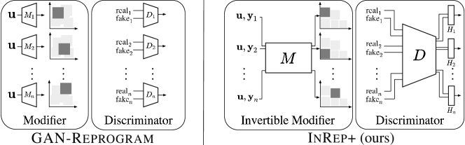
Figure 3: Highlights of design differences between GAN-Reprogram [29] and InRep+ (ours). GAN-Reprogram (left) learns a pair of modifier $M_{i}$ and discriminator $D_{i}$ per each of $n$ conditions. InRep+ (right) makes three improvements over GAN-Reprogram: i) using a single conditional modifier $M$ and sharing weights between $\{D_{i}\}_{1}^{n}$ to improve memory scalability when $n$ is large, ii) adopting the invertible architecture for modifier network $M$ to prevent class-conditional latent regions from overlapping, iii) replacing the standard GAN loss with a new PU-based loss to overcome the false rejection issue.

Weight-sharing architectures

For the modifier, we use only a single conditional modifier network $M$ for all classes. For the discriminator, we share a base network $D$ for all classes and design multiple linear heads $H_{y}$ on top of $D$, each head for a conditional class, that is, $D_{y}=H_{y}\circ D$. This design helps maintain the separation principle of input reprogramming while significantly reducing the number of trainable parameters and weights needed to store.

Invertible modifier network

The modifier network $M$ learns a mapping $\mathbb{R}^{d_{\mathbf{z}}}\to\mathbb{R}^{d_{{\mathbf{z}}_{y}}}$, where ${\mathbf{z}}$ is the input noise and ${\mathbf{z}}_{y}$ is the $y$-conditional noise. The input noise ${\mathbf{z}}$ is an aggregation of a random noise vector ${\mathbf{u}}$ and the label $y$ in the form of label embedding [2]. We use a learnable embedding module $E$ to convert each discrete label into a continuous vector with dimension $d_{\mathbf{y}}$. The use of label embedding instead of one-hot encoding has been shown to help GANs learn better [2]. Here, $d_{{\mathbf{z}}}=d_{\mathbf{u}}+d_{\mathbf{y}}$ with $d_{{\mathbf{z}}},d_{\mathbf{u}}$, and $d_{\mathbf{y}}$ being dimensions of ${\mathbf{z}}$, ${\mathbf{u}}$, and ${\mathbf{y}}$ respectively. In this work, we use the concatenation function as the aggregation function. To prevent outputs of modifiers on different classes from overlapping, we design the modifier to be invertible using the architecture of invertible neural networks [30, 31, 32]. Intuitively, the invertible modifier maps different random noises to different latent vectors, guaranteeing uniqueness. Notably, the use of invertibility leads to a dimension gap between the random noise ${\mathbf{u}}$ and the conditional noise ${\mathbf{z}}_{y}$ as $d_{\mathbf{u}}<d_{{\mathbf{z}}}=d_{{\mathbf{z}}_{y}}$. However, the small dimension gap does not significantly affect the performance of the modifier network on capturing the true distribution of the conditional latent because the underlying manifold of complex data usually has a much lower dimension in most practical cases [49]. Modifier $M$ needs to be sufficiently expressive to learn the target noise partitions while maintaining the computation efficiency.

Training conditional discriminator with Positive-Unlabeled learning

Assume that $G$ generates $y$-class data with probability $p_{\text{class}}(y)$. At the beginning of discriminator training, $p_{\text{class}}(y)$ fraction of generated samples are high-quality and in-class but labeled as fake by the discriminator. This results in the training instability of the existing GAN reprogramming approach [29]. To deal with this issue, we view the discriminator training through Positive-Unlabeled (PU) learning lens. PU learning has been studied in binary classification, where only a subset of the dataset is labeled with one particular class, and the rest is unlabeled [50, 51, 52]. Considering the generated data as unlabeled, we can cast the conditional discriminator learning as a PU learning problem: classifying positive (in-class and high-quality) data from unlabeled (generated) data.

Now, we consider training $(M_{y},D_{y})$ for a fixed $y$. As discussed, the distribution of generated data $G(M_{y}({\mathbf{u}}))$ can be viewed as a mixture of $p_{\text{data}}({\bm{x}}|y)$ and the residual distribution, say $p_{\text{gf}}({\bm{x}})$, where ‘g’ stands for generated and ‘f’ means that they should be labeled as fake because they are out-class. That is, letting $\pi_{y}$ be the fraction of $y$-class data among generated data, we have $p_{G(M_{y}({\mathbf{u}}))}({\bm{x}})=\pi_{y}\cdot p_{\text{data}}({\bm{x}}|y)+(1-\pi_{y})\cdot p_{\text{gf}}({\bm{x}})$. Given this decomposition, the ideal discriminator objective function is:

$$V_{y}^{PU} =\mathbb{E}_{\mathbf{x}\sim p_{\text{data}}({\bm{x}}|y)}\left[\log D_{y}({\mathbf{x}})\right]+\pi_{y}\mathbb{E}_{\mathbf{x}\sim p_{\text{data}}({\bm{x}}|y)}\left[\log(D_{y}({\mathbf{x}}))\right]+(1-\pi_{y})\mathbb{E}_{{\mathbf{x}}\sim p_{\text{gf}}({\bm{x}})}\left[\log(1-D_{y}({\mathbf{x}}))\right]$$ (1)

$$=(1+\pi_{y})\mathbb{E}_{\mathbf{x}\sim p_{\text{data}}({\bm{x}}|y)}\left[\log D_{y}({\mathbf{x}})\right]+\mathbb{E}_{{\mathbf{u}}\sim p_{{\mathbf{u}}}({\bm{u}})}\left[\log(1-D_{y}(G(M_{y}({\mathbf{u}}))))\right]-\pi_{y}\mathbb{E}_{\mathbf{x}\sim p_{\text{data}}({\bm{x}}|y)}\left[\log(1-D_{y}({\mathbf{x}}))\right]$$ (2)

where the last equation follows from $(1-\pi_{y})p_{\text{gf}}({\bm{x}})=p_{G(M_{y}({\mathbf{u}}))}({\bm{x}})-\pi_{y}p_{\text{data}}({\bm{x}}|y)$.

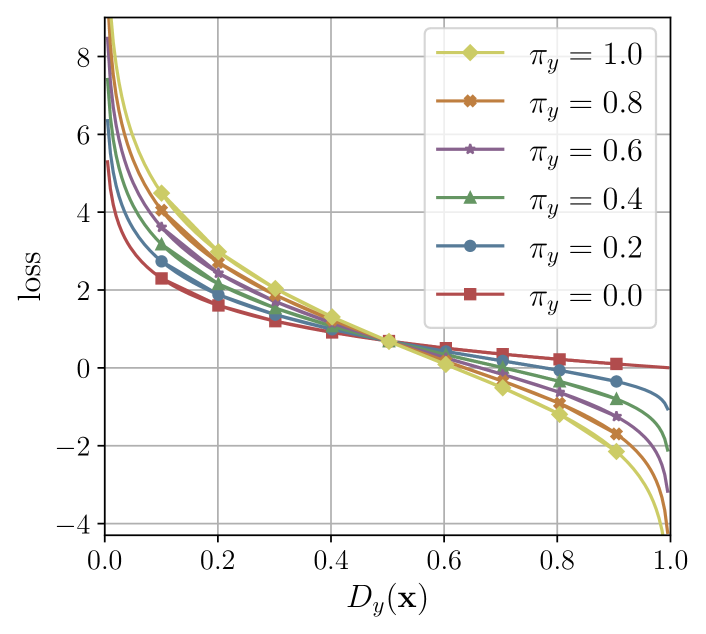
Figure 4: Visualization of InRep+’s discriminator loss on real data. We visualize the loss with different values of $\pi_{y}$ (in $[0,1]$) and $D_{y}(x)$ (in $[0,1]$). Compared to the standard negative log-loss ($\pi_{y}=0$), the new loss ($\pi_{y}>0$) more strongly encourages $D_{y}$ to predict values near $1$ for positive samples.

The discriminator loss is $-V_{y}^{PU}$. For real data $\mathbf{x}\sim p_{\text{data}}({\bm{x}}|y)$, discriminator minimizes a new loss $-(1+\pi_{y})\log(D_{y}({\mathbf{x}}))+\pi_{y}\log(1-D_{y}({\mathbf{x}}))$ instead of the standard negative log-loss $-\log(D_{y}({\mathbf{x}}))$. Fig. 4 visualizes this new loss with various values of $\pi_{y}$. Compared to the standard loss ($\pi_{y}=0$), our loss function strongly encourages the discriminator to assign positively labeled data higher scores that are very close to $1$. Also, when the prediction is close to $1$, the loss takes an unboundedly large negative value, indirectly assigning more weights to the first term in (2). If $\pi_{y}$ is close to $1$, the relative weights given to the real samples become even higher. An intuitive justification is that the loss computed on the generated data becomes less reliable when $\pi_{y}$ gets larger, so one should focus more on the loss computed on the real data.

Note that the last term in (1) is always negative as $D_{y}$ outputs a probability value, but its empirical estimate, shown in the sum of the last two terms in (2), may turn out to be positive due to finite samples. We correct this by clipping the estimated value to be negative as shown below:

We set $\pi_{y}=\tfrac{1}{|{\mathbb{Y}}|}$ initially when the generated data is well-balanced between classes, and gradually increase $\pi$ to $1$ by temperature scaling to capture the increasing fraction of $y$-class data.

Remark 1.

In the context of the UGAN training, recent work [33] studies a similar PU-based approach to address the training instability caused by the false rejection issue discussed above. However, unlike our approach, their approach does not consider the term $\mathbb{E}_{{\mathbf{x}}\sim p_{\text{data}}({\bm{x}}|y)}\left[\log D_{y}({\mathbf{x}})\right]$ in their loss function design. This design makes their loss function invalid when $\pi_{y}$ is close to $0$, that is, at the beginning of GAN training. On the other hand, our loss function is valid for all $\pi_{y}\in[0,1]$. We also note that the false rejection issue is more relevant near the end of the standard GAN training when the generated samples are more similar to the real ones, while it occurs right at the beginning of GAN conditioning training. This difference leads to different uses of the PU-based loss for the standard GAN and GAN conditioning.

Input: Pretrained unconditional generator $G$, class-conditional dataset ${\mathbb{D}}$ with label set $\mathbb{Y}$, noise dimension $d$, batch size $m$, learning rates $\alpha,\beta$, number of discriminator steps $k$, number of training iterations $t$

Result: Class-conditional generator $G^{\prime}$

Initialize parameters: ${\bm{\theta}}_{M}$ for modifier network $M$, ${\bm{\theta}}_{E}$ for embedding module $E$, ${\bm{\theta}}_{D}$ for discriminator network $D$, and $\{{\bm{\theta}}_{y}:y\in{\mathbb{Y}}\}$ for linear heads $\{H_{y}:y\in{\mathbb{Y}}\}$.

Let $D_{y}=H_{y}(D(\cdot;{\bm{\theta}}_{D});{\bm{\theta}}_{y})$, ${\bm{w}}_{D_{y}}=[{\bm{\theta}}_{D},{\bm{\theta}}_{y}]$ for each $y\in{\mathbb{Y}}$, ${\bm{w}}_{EM}=[{\bm{\theta}}_{M},{\bm{\theta}}_{E}]$

for $t$ iterations do

       for $k$ steps do

             sample $\{{\mathbf{x}}_{i},{\textnormal{y}}_{i}\}_{i=1}^{m}\sim{\mathbb{D}}$, $\{{\mathbf{u}}_{i}\}_{i=1}^{m}\sim\mathcal{N}(\mathbf{0},{\bm{I}}_{d})$

             ${\mathbf{y}}_{i}=E({\textnormal{y}}_{i};{\bm{\theta}}_{E})$ for all $i$;   $\tilde{{\mathbf{x}}}_{i}\leftarrow G(M({\mathbf{u}}_{i},{\mathbf{y}}_{i};{\bm{\theta}}_{M}))$ for all $i$

             for each $y\in{\mathbb{Y}}$ do

                   $V_{y}^{(i)}\leftarrow V_{y}^{PU}(\tilde{{\mathbf{x}}}_{i},{\mathbf{x}}_{i})$ for all $i$

                   $\nabla_{{\bm{w}}_{D_{y}}}=\text{Adam}(\nabla_{{\bm{w}}_{D_{y}}}\frac{1}{m}\sum_{i=1}^{m}{V_{y}^{(i)}})$;   ${\bm{w}}_{D_{y}}\leftarrow{\bm{w}}_{D_{y}}+\alpha\nabla_{{\bm{w}}_{D_{y}}}$

            

      sample $\{\hat{{\mathbf{u}}}_{i}\}_{i=1}^{m}\sim\mathcal{N}(\mathbf{0},{\bm{I}}_{d})$

       for each $y\in{\mathbb{Y}}$ do

             ${\mathbf{y}}=E(y;{\bm{\theta}}_{E})$; $\hat{{\mathbf{x}}}_{i}\leftarrow G(M(\hat{{\mathbf{u}}}_{i},{\mathbf{y}};{\bm{\theta}}_{M}))$ for all $i$;   $V_{y}^{(i)}\leftarrow V_{y}^{PU}(\tilde{{\mathbf{x}}}_{i},{\mathbf{x}}_{i})$ for all $i$

             $\nabla_{{\bm{w}}_{EM}}=\text{Adam}(-\nabla_{{\bm{w}}_{EM}}\frac{1}{m}\sum_{i=1}^{m}V_{y}^{(i)})$;   ${\bm{w}}_{EM}\leftarrow{\bm{w}}_{EM}+\beta\nabla_{{\bm{w}}_{EM}}$

      

$G^{\prime}(\cdot,\cdot)\leftarrow G\circ M(\cdot,E(\cdot;{\bm{\theta}}_{E});{\bm{\theta}}_{M})$

Algorithm 1 InRep+

3.3 InRep+’s optimality under ideal setting

In this section, we highlight that the GAN’s global equilibrium theorem [1] still holds under the PU-learning principle incorporated in the discriminator training. Specifically, InRep+ attains the global equilibrium if and only if generated samples follow the true conditional distribution. This theorem guarantees that InRep+ learns the exact conditional distribution under the ideal training. We provide the proofs for the proposition and the theorem in Appendix A.3.

Proposition 1.

Fix the ideal unconditional generator $G$ and arbitrary modifier $M_{y}$, the optimal discriminator for $y$ is

$$D_{y}^{*}(M_{y}({\mathbf{u}}))=\frac{(1+\pi_{y})p_{\text{data}}({\bm{x}}|y)}{(1+\pi_{y})p_{\text{data}}({\bm{x}}|y)+(1-\pi_{y})p_{\text{gf}}({\bm{x}})}.$$

The proposition shows that the optimal discriminator $D^{*}$ learns a certain balance between $p_{\text{data}}({\bm{x}}|y)$ and $p_{\text{gf}}({\bm{x}})$. Fixing such an optimal discriminator, we can prove the equilibrium theorem.

Theorem 1 (Adapted from [1]).

When the ideal unconditional generator $G^{*}$ and discriminator $D^{*}$ are fixed, the globally optimal modifier is attained if and only if $p_{\text{gf}}({\bm{x}})=p_{G(M_{y}({\mathbf{u}}))}({\bm{x}})=p_{\text{data}}({\bm{x}}|y)$.

4 Experiments

In this section, we first describe our experiment settings, including datasets, baselines, evaluation metrics, network architectures, and the training details. In Sec. 4.1, we present conditioned samples from InRep+ on various data. In Sec. 4.2, we quantify the learning ability of InRep+ varying the amount of labeled data on different datasets. In Sec. 4.3, we evaluate the robustness of InRep+ in settings of class-imbalanced and label-noisy labeled data. We also conduct an ablation study on the role of InRep+’s components (Sec. 4.4). Our code and pretrained models are available at https://github.com/UW-Madison-Lee-Lab/InRep.

Datasets and baselines

We use a synthetic Gaussian mixture dataset (detailed in Sec. 4.1) and various real datasets: MNIST [53], CIFAR10 [54], CIFAR100 [54], Flickr-Faces-HQ (FFHQ) [55], CelebA [56]. Our baselines are GAN-Reprogram [29], fine-tuning [25, 26], and three popular standard CGANs (ACGAN, ProjGAN, and ContraGAN). Fine-tuning is a combined approach of TransferGAN [25] and MineGAN [26], which first learns a discriminator and a miner network given the condition set [26], then fine-tunes all networks using ACGAN loss.

Evaluation metrics

We use the popular Fréchet Inception Distance (FID) [57] and recall [58] to measure the quality and diversity of learned distributions. FID measures the Wasserstein-2 (Fréchet) distance between the learned and true distributions in the feature space of the pretrained Inception-v3 model. Lower FID indicates better performance. To measure the conditioning performance, we use Intra-FID [2] and Classification Accuracy Score (CAS) [59, 60, 61]. Specifically, Intra-FID is the average of FID scores measured separately on each class, and CAS is the testing accuracy on the real data of the classifier trained on the generated data.

Network architectures and training

Our architectures and configurations of networks are mainly based on GANs’ best practices [3, 4, 62, 63]. We adopt the same network architectures for all models. For InRep+, we set the dimension of label embedding vectors to $10$ for all experiments. Our modifier network uses the i-ResNet architecture [31], with three layers for simple datasets (Gaussian mixture, MNIST, CIFAR10) and five layers for more complex datasets (CIFAR100, FFHQ). We design the modifier networks to be more lightweight than generators and discriminators. For instance, our modifier for CIFAR10 has only $0.1$M parameters while the generator and the discriminator have $4.3$M and $1$M parameters, respectively. The latent distribution is the standard normal distribution with $128$ dimensions. For training, we employ Adam optimizer with the learning rates of $2\cdot 10^{-4}$ and $2\cdot 10^{-5}$ for modifier and discriminator networks. $\beta_{1},\beta_{2}$ are $0.5,0.999$, respectively. We train $100\,000$ steps with five discriminator steps before each generator step. InRep+ takes much less time compared to other approaches. For instance, training ACGAN and ContraGAN on CIFAR10 may take up to several hours, while training InRep+ takes approximately half of an hour to achieve the best performance. For implementation, we adopt the widely used third-party GAN library [4] with PyTorch implementations for reliable and fair assessments. We run our experiments on two RTX8000 (48 GB memory), two TitanX (11GB), two 2080-Ti (11GB) GPUs. For pretrained unconditional generators, we mostly pretrain unconditional generators on simple datasets (Gaussian mixture, MNIST, CIFAR10, CIFAR100), and make use of large-scale pretrained models for StyleGAN trained on FFHQ. We provide more details in Appendix B.

4.1 Performing GAN conditioning with InRep+ on various data

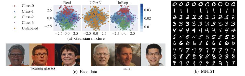
Figure 5: Conditional samples from InRep+ on different datasets. (a) Gaussian mixture: We synthesize a mixture of four Gaussian distributions on two-dimensional space with $10\,000$ samples. Four Gaussian components have unit variance and their means are $(0,2),(-2,0),(0,-2),(2,0)$, respectively. The synthesized data is visualized in the left figure (Real). The central figure visualizes the distribution learned by unconditional GAN (UGAN). The right figure (InRep+) shows the conditional samples from InRep+. As we can see, the InRep+’s distribution is highly similar to the real data distribution. Also, it covers all four distribution modes. (b) MNIST: We visualize class-conditional samples of CGANs learned by InRep+, each row per class. Our samples have correct labels, with high-quality and diverse shapes. (c) Face data: Unconditional GAN model is StyleGAN pretrained on the FFHQ dataset, which contains high-resolution face images. We use CelebA data as the labeled data, with two classes: wearing glasses and male. Most conditional samples are high-quality and with correct labels. We further show conditional samples of CIFAR10 in Fig. 6.

Fig. 5 visualizes conditional samples of CGANs learned by InRep+ on different datasets: Gaussian mixture, MNIST, and the face dataset. Shown in Fig. 5a are samples on Gaussian mixture data. We synthesize a dataset of $10\,000$ samples drawn from the Gaussian mixture distribution with four uniformly weighted modes in 2D space, depicted on the left of the figure (Real). Four components have unit variance with means $(0,2),(-2,0),(0,-2),(2,0)$, respectively. As seen in the figure, generated distribution from InRep+ covers all four modes of data and shares a similar visualization with the real distribution. For MNIST (Fig. 5b), each row represents a class of generated conditional samples. We see that all ten rows have correct images with high quality and highly diverse shapes. Similarly, Fig. 5c shows two classes (wearing glasses and male) of high-resolution face images, which are generated using InRep+’s conditional generator. In this setting, UGAN is the StyleGAN model [55] pretrained on the unlabeled FFHQ data, and labeled data is the CelebA data. For CIFAR10, the last row of Fig. 6 shows our conditional samples from InRep+ with different levels of supervision. These visualizations show that InRep+ is capable of well-conditioning GANs correctly.

4.2 GAN conditioning with different levels of supervision

Method	Class	1%	10%	20%	50%	100%
CGAN (ACGAN)	airplane automobile bird
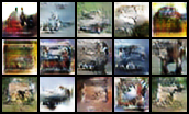
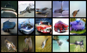
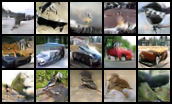
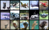
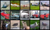
CGAN (ProjGAN)	airplane automobile bird
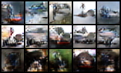
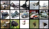
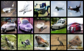
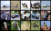
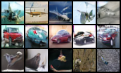
CGAN (ContraGAN)	airplane automobile bird
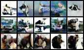
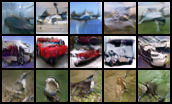
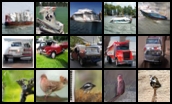
Fine-tuning	airplane automobile bird
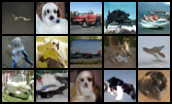
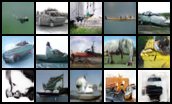
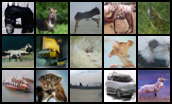
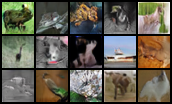
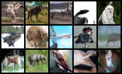
GAN-Reprogram	airplane automobile bird
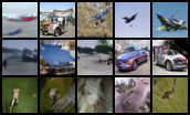
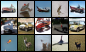
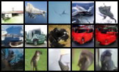
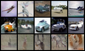
InRep+ (ours)	airplane automobile bird

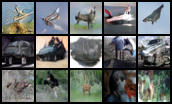
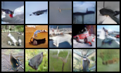
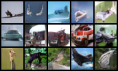
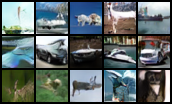
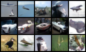
Figure 6: CIFAR10 conditional images from GAN conditioning methods. We compare the samples in terms of quality and class-correctness, varying amounts of labeled data. A row of each figure represents images conditioned on one of three classes: airplane, automobile, bird (top to bottom). At $1$% and $10$%, samples from ACGAN, ProjGAN, and CGAN are blurrier and in lower resolutions than those of methods reusing UGAN (InRep+, fine-tuning, and GAN-Reprogram). Furthermore, InRep+’s samples have both high quality and correct labels while some samples from GAN-Reprogram and fine-tuning methods have incorrect classes. When more labeled data is provided (20%, 50%, 100%), CGAN algorithms (ACGAN, ProjGAN, and ContraGAN) gradually synthesize samples with higher quality and correctly conditioned classes. Noticeably, while all samples of ContraGAN models have high quality, some of them are mistakenly conditioned. This behavior probably causes higher Intra-FID scores in spite of low FID scores. Among methods reusing UGANs, most samples from InRep+ have both high quality and correct classes, while GAN-Reprogram and the fine-tuning method show more wrong-class conditional samples.

Table 2: FID and Intra-FID evaluations. We compare InRep+ with baselines on CIFAR10 and CIFAR100 under various amounts of labeled data (x% on CIFAR10 means that x% of labeled CIFAR10 is randomly selected). When the labeled dataset is small (1%, 10%), InRep+ outperforms baselines, shown in the smallest FID and Intra-FID scores over all datasets. As more labeled data is given, directly applying CGANs results in better performances (lower FID and Intra-FID). InRep+ maintains small FID gaps to best models. Values of GAN-Reprogram and standard deviations on CIFAR100 are not obtained due to the computing limitation.

Dataset	Method	FID ($\downarrow$)						Intra-FID ($\downarrow$)
		1%	10%	20%	50%	100%		1%	10%	20%	50%	100%
CIFAR10	CGAN (ACGAN)	$69.01$$\mathrm{p}\mathrm{m}$0.28	$30.55$$\mathrm{p}\mathrm{m}$0.45	$21.50$$\mathrm{p}\mathrm{m}$0.14	$16.10$$\mathrm{p}\mathrm{m}$1.37	$12.38$$\mathrm{p}\mathrm{m}$2.76		$141.71$$\mathrm{p}\mathrm{m}$0.33	$88.33$$\mathrm{p}\mathrm{m}$0.15	$73.47$$\mathrm{p}\mathrm{m}$0.55	$68.24$$\mathrm{p}\mathrm{m}$2.47	$54.86$$\mathrm{p}\mathrm{m}$8.65
	CGAN (ProjGAN)	$67.54$$\mathrm{p}\mathrm{m}$0.22	$30.35$$\mathrm{p}\mathrm{m}$0.88	$21.21$$\mathrm{p}\mathrm{m}$ 0.14	$14.81$$\mathrm{p}\mathrm{m}$ 0.11	$11.86$$\mathrm{p}\mathrm{m}$ 1.86		$124.35$$\mathrm{p}\mathrm{m}$0.62	$84.41$$\mathrm{p}\mathrm{m}$1.91	$67.13$$\mathrm{p}\mathrm{m}$0.23	$58.77$$\mathrm{p}\mathrm{m}$0.27	$52.16$$\mathrm{p}\mathrm{m}$0.86
	CGAN (ContraGAN)	$43.11$$\mathrm{p}\mathrm{m}$3.28	$29.44$$\mathrm{p}\mathrm{m}$1.73	$25.53$$\mathrm{p}\mathrm{m}$0.49	$12.44$$\mathrm{p}\mathrm{m}$0.16	$12.19$$\mathrm{p}\mathrm{m}$0.14		$271.79$$\mathrm{p}\mathrm{m}$6.56	$155.29$$\mathrm{p}\mathrm{m}$7.12	$145.07$$\mathrm{p}\mathrm{m}$8.37	$132.97$$\mathrm{p}\mathrm{m}$8.90	$132.43$$\mathrm{p}\mathrm{m}$0.44
	Fine-tuning	$22.01$$\mathrm{p}\mathrm{m}$0.19	$15.97$$\mathrm{p}\mathrm{m}$0.70	$16.13$$\mathrm{p}\mathrm{m}$0.17	$15.40$$\mathrm{p}\mathrm{m}$0.58	$13.98$$\mathrm{p}\mathrm{m}$1.12		$117.85$$\mathrm{p}\mathrm{m}$0.16	$108.00$$\mathrm{p}\mathrm{m}$0.55	$99.44$$\mathrm{p}\mathrm{m}$0.19	$92.02$$\mathrm{p}\mathrm{m}$11.36	$90.11$$\mathrm{p}\mathrm{m}$6.29
	GAN-Reprogram	$23.12$$\mathrm{p}\mathrm{m}$3.47	$22.62$$\mathrm{p}\mathrm{m}$0.33	$19.81$$\mathrm{p}\mathrm{m}$0.12	$16.27$$\mathrm{p}\mathrm{m}$0.16	$15.45$$\mathrm{p}\mathrm{m}$0.37		$114.51$$\mathrm{p}\mathrm{m}$1.33	$78.04$$\mathrm{p}\mathrm{m}$5.51	$74.40$$\mathrm{p}\mathrm{m}$6.47	$67.52$$\mathrm{p}\mathrm{m}$5.05	$68.32$$\mathrm{p}\mathrm{m}$5.14
	InRep+ (ours)	$16.39$$\mathrm{p}\mathrm{m}$1.37	$14.52$$\mathrm{p}\mathrm{m}$0.97	$14.84$$\mathrm{p}\mathrm{m}$1.22	$13.45$$\mathrm{p}\mathrm{m}$3.18	$12.99$$\mathrm{p}\mathrm{m}$1.21		$76.24$$\mathrm{p}\mathrm{m}$3.35	$65.45$$\mathrm{p}\mathrm{m}$3.25	$62.19$$\mathrm{p}\mathrm{m}$3.22	$61.81$$\mathrm{p}\mathrm{m}$1.34	$59.62$$\mathrm{p}\mathrm{m}$2.21
CIFAR100	CGAN (ACGAN)	$83.09$	$33.40$	$38.15$	$23.78$	$17.48$		$256.37$	$230.41$	$207.10$	$191.54$	$191.35$
	CGAN (ProjGAN)	$99.54$	$42.28$	$24.91$	$22.22$	$13.90$		$256.61$	$212.70$	$196.53$	$175.59$	$170.55$
	CGAN (ContraGAN)	$74.34$	$47.89$	$31.59$	$17.19$	$13.45$		$256.69$	$213.73$	$216.42$	$200.58$	$208.18$
	Fine-tuning	$25.87$	$18.43$	$17.64$	$15.57$	$14.45$		$249.77$	$249.72$	$237.16$	$239.64$	$236.70$
	InRep+ (ours)	$20.22$	$18.42$	$17.87$	$17.04$	$16.92$		$238.24$	$207.18$	$202.28$	$201.19$	$187.09$

Table 3: Recall and CAS evaluations on CIFAR10. We measure GAN conditioning performance with recall and CAS varying amounts of labeled data (x% on CIFAR10 means that x% of labeled CIFAR10 is randomly selected). InRep+ outperforms baselines in terms of recall and CAS when small amounts of labeled data (1%, 10%, 20%) are available. The performance gap between InRep+ and others becomes larger as less supervision is provided. When more labeled data is provided (50%, 100%), InRep+ performs competitively to the best models in terms of recall and still outperforms others in terms of CAS.

Method	Recall ($\uparrow$)					CAS ($\uparrow$)
	1%	10%	20%	50%	100%	1%	10%	20%	50%	100%
CGAN (ACGAN)	$0.12$	$0.59$	$0.66$	$0.72$	$0.78$	$11.63$	$29.83$	$33.04$	$39.70$	$43.99$
CGAN (ProjGAN)	$0.12$	$0.56$	$0.67$	$0.72$	$0.80$	$21.52$	$28.09$	$30.03$	$32.43$	$35.06$
CGAN (ContraGAN)	$0.23$	$0.59$	$0.67$	$0.79$	$0.77$	$12.00$	$14.50$	$15.02$	$21.91$	$18.78$
Fine-tuning	$0.64$	$0.76$	$0.77$	$0.77$	$0.79$	$11.50$	$12.68$	$15.75$	$15.56$	$15.66$
GAN-Reprogram	$0.65$	$0.69$	$0.72$	$0.75$	$0.76$	$21.08$	$23.95$	$26.94$	$27.56$	$29.64$
InRep+ (ours)	$0.72$	$0.77$	$0.78$	$0.78$	$0.79$	$22.03$	$31.37$	$35.19$	$47.80$	$46.38$

We compare GAN conditioning methods under different amounts of labeled data. Specifically, we use different proportions of the training dataset (1%, 10%, 20%, 50%, and 100%) as the labeled data. Table 2 shows the comparison in terms of FID and Intra-FID on CIFAR10 and CIFAR100 datasets. Table 3 provides additional measures (recall and CAS scores) of the methods on CIFAR10. We also compare the quality of conditional samples on CIFAR10 in Fig. 6.

InRep+ outperforms baselines in the regime of low supervision.

When the supervision level is $10$% or less, InRep+ consistently achieves the best scores (FID and Intra-FID) over all datasets. For instance, FID scores of InRep+ at 1% are $16.39$ and $20.22$ for CIFAR10 and CIFAR100 (Table 2). The corresponding Intra-FID scores of InRep+ are $76.24$ and $238.24$, showing large gaps ($38.27$ and $11.53$) to the second-best models. Notably, these score gaps between InRep+ and other models become larger as less supervision is provided. Regarding recall and CAS metrics on CIFAR10, Table 3 also supports our findings: InRep+ outperforms baselines in both recall and CAS when small amounts of labeled data are available.

We attribute good performances of InRep+ to its design that utilizes the representation of trained generators and efficiently uses limited labels in separating conditional latent vectors (Sec. 3.2). Interestingly, thanks to well-trained generators, GAN-Reprogram and fine-tuning also achieve better performances than other CGANs. For the qualitative comparison, Fig. 6 partly illustrates that most samples from InRep+ have higher image quality than those from CGAN methods and are more correctly conditioned than samples from fine-tuning and GAN-Reprogram.

As more labeled data is provided (20% and more), CGANs gradually obtain better scores and outperform InRep+, but InRep+ manages to keep relatively small gaps to the best CGANs. For instance, with full supervision on CIFAR10, these gaps between InRep+ and the best model, ProjGAN, are just $1.1$ and $7.5$ in terms of FID and Intra-FID.

4.3 Robustness to class-imbalanced data and noisy supervision

We analyze two practical settings of the labeled data, when the data is class-imbalanced and when the labels are noisy.

Table 4: FID evaluation on class-imbalanced CIFAR10. The dataset has 10 classes where classes $0$ and $1$ are minor. Compared to the FID on class-balanced data (Table 2), InRep+ and GAN-Reprogram obtain the smallest FID increases among methods, indicating that they are less affected by the imbalance in labels. Also, InRep+ achieves the best Intra-FIDs for minor classes, close to the average score of major classes, while the Intra-FID gaps between the minor and major classes are larger in other models.

Method	FID ($\downarrow$)	Intra-FID ($\downarrow$)
		Class 0	Class 1	Major classes
CGAN (ACGAN)	$19.87$	$124.25$	$141.89$	$89.29$
CGAN (ProjGAN)	$14.80$	$75.87$	$80.59$	$53.13$
CGAN (ContraGAN)	$18.95$	$139.75$	$84.20$	$135.08$
Fine-tuning	$14.43$	$117.52$	$100.03$	$89.29$
GAN-Reprogram	$16.01$	$73.06$	$88.92$	$68.59$
InRep+ (ours)	$13.26$	$69.48$	$61.68$	$60.06$

InRep+ outperforms GAN conditioning baselines on class-imbalanced CIFAR10

The class-imbalanced CIFAR10 has two minor classes ($0$ and $1$) that use 10% of their labeled data, while other classes remain unchanged. Training on this augmented dataset, we observe that InRep+ obtains the lowest overall FID ($13.26$), shown in Table 4. InRep+ also achieves the best Intra-FID scores for both two minor classes ($69.48$ and $61.68$), which are close to the average Intra-FID of major classes ($60.06$). On the other hand, other methods show larger gaps between Intra-FID of minor classes and the average Intra-FID of major classes. For instance, these score gaps in ProjGAN and ACGAN are all greater than $20$. This result validates the advantage of InRep+ in learning with class-imbalanced labeled data.

Remark 2 (Fairness in the data generation).

The under-representation of minority classes in training data may bias models towards generating samples with more features of majority classes or samples of minority classes with lower quality and less diversity [64, 65, 66]. Being more robust against the class imbalance, InRep+ is a promising candidate for GAN conditioning with fair generation.

InRep+ is more robust to label noises in CIFAR10

Table 5: FID evaluation on label-noisy CIFAR10. The label-noisy CIFAR10 is constructed by corrupting labels of CIFAR10 with asymmetric noises. Compared to reported scores on the label-clean data (Table 2), InRep+ and GAN-Reprogram maintain small FIDs (13.15 and 15.84) and Intra-FIDs (63.15 and 71.51) under the label corruption, while other methods suffer from high increases. For instance, the increased Intra-FID gaps of ACGAN and ProjGAN are all greater than 30. Furthermore, InRep+ and GAN-Reprogram also maintain the smallest Intra-FIDs for both noisy and clean classes. These results indicate that input reprogramming approaches are more robust against label noises.

Method	FID ($\downarrow$)	Intra-FID ($\downarrow$)
		All classes	Noisy classes	Clean classes
CGAN (ACGAN)	$27.63$	$129.11$	$140.64$	$121.42$
CGAN (ProjGAN)	$15.44$	$86.85$	$91.30$	$83.90$
CGAN (ContraGAN)	$14.10$	$149.49$	$96.49$	$184.83$
Fine-tuning	$16.18$	$115.91$	$125.52$	$106.00$
GAN-Reprogram	$15.84$	$71.51$	$73.10$	$69.92$
InRep+ (ours)	$13.15$	$63.15$	$65.93$	$61.30$

We adopt the class-dependent noise setting in robust image classification [67, 68], and corrupt clean labels with flipping probability $0.4$ as follows: bird $\to$ airplane, cat $\to$ dog, deer $\to$ horse, truck $\to$ automobile. Shown in Table 5 are evaluated FID and Intra-FID. Though label corruption causes FID increases in all models, the increase of InRep+ is only $0.16$ (compared to clean-label FID in Table 2), comparable to GAN-Reprogram and stark contrast with large gaps of CGAN methods. In terms of Intra-FID, InRep+ achieves the smallest score ($63.15$), and enjoys the smallest Intra-FID increases together with GAN-Reprogram ($3.5$ and $3.2$) among evaluated methods. Also, their clean classes are less affected by label noises, while we observe non-negligible deviations in other models. These results show the strong robustness of input reprogramming methods against label noises. We attribute this robustness to their modular design, which preserves the representation learned by unconditional generators and focuses on learning the conditional distribution. Also, the multi-head design of the conditional discriminator contributes to preserving the separation between data of different classes. Thus, corrupted labels only significantly affect the corresponding classes in InRep+ (and GAN-Reprogram) while affecting all classes in the joint training of other methods (CGANs and fine-tuning).

4.4 Ablation study

Table 6: Analyzing the effect of InRep+’s components. Each row compares InRep+ (w/ PU-loss) with its version without PU-based loss (w/ PU-loss). Each column compares InRep+ (w/ invertibility) with its version when the modifier network is not invertible (w/o invertibility). The scores are Intra-FID on CIFAR10. Both two components help improve InRep+. Enabling invertibility reduces Intra-FID by nearly $11.7$ and $15.1$, while enabling the PU-based loss improves approximately $2.9$ and $6.3$. These results indicate the stronger effect of the invertibility than the PU-based loss on the final performance of InRep+.

Setting	w/ PU-loss	w/o PU-loss
w/ invertibility	64.25	67.14
w/o invertibility	75.92	82.26

We investigate the empirical effect of the invertible architecture and the PU-based loss on InRep+. We construct four InRep+ versions from enabling or disabling each of two components. We use ResNet architecture [69] and the standard GAN loss as replacements for the i-ResNet architecture and our PU-based loss. UGAN is pretrained on unlabeled CIFAR10, and the labeled data is $10\%$ of CIFAR10 (to observe better the effect of PU-based loss under the low-label regime). Shown in Table 6 are the Intra-FID scores of four models. The original InRep+ achieves the best score ($64.25$), while removing all components causes a higher Intra-FID ($82.26$). Using PU-based loss and invertibility help InRep+ reduce Intra-FID, with the biggest decreases being $6.3$ and $15.1$, respectively. Thus both components have positive effects on the InRep+’s performance, and invertibility shows a higher impact on InRep+.

5 Discussion

Limitation

InRep+ depends greatly on the pretrained unconditional generator: how perfectly the unconditional generator learns the underlying data distribution and how well its latent space organizes. The latest research [3, 70] observes the existing capacity gaps between unconditional GANs and conditional GANs on large-scale datasets. Therefore, how to improve InRep+ on large-scale datasets is still a challenging problem, especially when GANs’ latent space structure has still not been well-understood. We leave this open problem for future work.

Beyond GAN: Can we apply InRep+ to other generative models?

Our work currently focuses on GANs for studying GAN conditioning because GANs attain state-of-the-art performances in various fields [3, 4, 5, 6, 7, 8], and numerous well-trained GAN models are publicly available. Nevertheless, InRep+ can be applied to other unconditional generative models. We can replace the unconditional generator from UGAN with one from other generative models, such as Normalizing Flows (Glow [71]) or Variational Autoencoders (VAEs) [72]. Interestingly, we notice that GAN training (as of InRep+) using generators pretrained on VAEs probably helps stabilize the training, reducing the mode collapse issue [73].

Enhancing input reprogramming to prompt tuning

Text prompts, which are textual descriptions of downstream tasks and target examples, have been shown to be effective at conditioning the GPT-3 model [12]. Multiple works have been proposed to design and adapt prompts for different linguistic tasks, such as prompt tuning [74] and prefix tuning [75]. The latter approach freezes the generative model and learns the prefix activations in the encoder stack. Sharing similar merit to prompt tuning, InRep+ can be a promising solution for learning better prompts in conditioning generative tasks while achieving significant computing savings by freezing the generative model.

6 Conclusion

In this study, we define the GAN conditioning problem and thoroughly review three existing approaches to this problem. We focus on input reprogramming, the best performing approach under the regime of scarce labeled data. We propose InRep+ as a new algorithm for improving the existing input reprogramming algorithm over critical issues identified in our analysis. In InRep+, we adopt the invertible architecture for the modifier network and a multi-head design for the discriminator. We derive a new GAN loss based on the Positive-Unlabeled learning to stabilize the training. InRep+ exhibits remarkable advantages over the existing baselines: The ideal InRep+ training provably learns true conditional distributions with perfect unconditional generators, and InRep+ empirically outperforms others when the labeled data is scarce, as well as bringing more robustness against the label noise and the class imbalance.

In (A), we present full statements, proofs, and examples for all propositions, lemmas, and theorems in the main paper.

In (B), we present the details of the experiments’ setting, including architectures, datasets, and evaluation metrics.

Appendix A Full Statements, Proofs, and Examples

A.1 Full statements and proofs for Section 2

A.1.1 Examples of the failure of ACGAN

ACGAN has two objective terms $L_{S},L_{C}$, modeling log-likelihoods of samples being from real data (by unconditional discriminator $D:{\mathbb{X}}\mapsto\{\real,\textrm{fake}\}$) and being from correct classes (by auxiliary classifier $D_{\textrm{aux}}:{\mathbb{X}}\mapsto{\mathbb{Y}}$), respectively. Then, the discriminators $(D,D_{\textrm{aux}})$ and generator $G$ maximize $\lambda L_{C}+L_{S}$, $\lambda L_{C}-L_{S}$ respectively with a regularization coefficient $\lambda$. As in the vanilla GANs, $L_{S}$ term encourages $G,D$ to learn the true (that is, unbiased) distribution, while $L_{C}$ term prefers easy-to-classify (that is, possibly biased) distributions. Therefore, $G$ might be able to maximize $\lambda L_{C}-L_{S}$ by learning a biased distribution (increased $L_{C}$) at the cost of compromised generation quality (increased $L_{S}$). Indeed, this phenomenon was observed in [40], where the authors provided theoretical reasons and empirical evidence that ACGAN-generated data are biased. We corroborate their finding by providing two examples in which ACGAN provably learns a biased distribution. For simplicity, we consider the Wasserstein GAN version [14] of ACGAN (W-GAN).

Lemma 1 (W-ACGAN fails to learn a correct Gaussian mixture, full statement).

Consider $1$-dimensional real data ${\textnormal{x}}\sim\mathcal{N}(y,1)$ where $y=2\operatorname{Bern}(1/2)-1$. Assume the perfect discriminator and the following generator, parameterized by $v$: $G({\mathbf{z}},y)\sim\mathcal{N}(y,v^{2}),v\in\mathbb{R}_{+}$ for given label $y$, that is, the only model parameter is the standard deviation $v$. Let $v^{*}(\lambda)$ be the optimal generator’s parameter that maximizes $\lambda L_{C}-L_{S}$. Then, $v^{*}(\lambda)\to 0$ as $\lambda\to\infty$.

Proof.

Recall that $L(v,\lambda)=\lambda L_{C}-L_{S}$ for the generator. From the fact that the $2$-Wasserstein distance between two Gaussian random variables is

$$W_{2}(\mathcal{N}(m_{1},\sigma_{1}^{2}),\mathcal{N}(m_{2},\sigma_{2}^{2}))=\sqrt{(m_{1}-m_{2})^{2}+(\sigma_{1}-\sigma_{2})^{2}},$$

the term $L_{S}$ reduces to a simple expression $\mathbb{E}_{{\textnormal{y}}}[W_{2}({\textnormal{x}},G({\mathbf{z}},{\textnormal{y}}))]=|1-v|$. Therefore, when there is no auxiliary discriminator, maximizing $L(v,\lambda)$ is indeed the same as minimizing $L_{S}$. Then, the ACGAN will find the global minimum $v^{*}=1$ via gradient descent as $L_{S}$ is convex. We will show that this is no longer true if we consider the auxiliary classification term $L_{C}$.

Consider the $L_{C}$ term that also has a closed-form expression:

$$\mathbb{E}_{{\textnormal{x}}}\left[\bm{1}_{\{D_{\textrm{aux}}({\textnormal{x}})={\textnormal{y}}\}}\right]+\mathbb{E}_{{\mathbf{z}},{\textnormal{y}}}\left[\bm{1}_{\{D_{\textrm{aux}}(G({\mathbf{z}},{\textnormal{y}}))={\textnormal{y}}\}}\right]$$

$$=2-\left(\frac{1}{2}\int_{0}^{\infty}p(x|y=-1)\mathop{}\!\mathrm{d}x+\frac{1}{2}\int_{-\infty}^{0}p(x|y=1)\mathop{}\!\mathrm{d}x\right)-\left(\frac{1}{2}\int_{0}^{\infty}p(G({\bm{z}},y)|y=-1)\mathop{}\!\mathrm{d}x+\frac{1}{2}\int_{-\infty}^{0}p(G({\bm{z}},y)|y=1)\mathop{}\!\mathrm{d}x\right)$$

$$=2-\frac{1}{2}Q(1)-\frac{1}{2}Q(1)-\frac{1}{2}Q(v^{-1})-\frac{1}{2}Q(v^{-1})=2-Q(1)-Q(v^{-1}),$$

where $Q(\cdot)$ is the complementary cumulative distribution function of the standard Gaussian, that is, $Q(t)=\int_{t}^{\infty}\mathcal{N}(\tau;0,1)d\tau$.

Therefore, the overall objective of the ACGAN to be minimized by $G$ is

$$L(v,\lambda)=|1-v|+\lambda\left(Q(1)+Q(v^{-1})\right)+const.$$

To see the behavior of the best generator, that is, $v^{*}=v^{*}(\lambda)$, first assume $v<1$. Using the chain rule and the property of $Q$ function that $\tfrac{d}{\mathop{}\!\mathrm{d}t}Q(t)=-\tfrac{1}{\sqrt{2\pi}}\exp(-t^{2}/2)$,

$$\frac{\partial L}{\partial v}=-1+\frac{\lambda}{\sqrt{2\pi}}\exp\left(-\frac{1}{2v^{2}}\right)\frac{1}{v^{2}}~{}~{}~{}\textrm{for }v<1.$$

As $\exp(-\tfrac{1}{2v^{2}})\tfrac{1}{v^{2}}$ is positive on $(0,1)$, the derivative is positive on $(0,1)$ as well by taking a large $\lambda$. Therefore, the generator will learn $v^{*}(\lambda)\to 0$ as $\lambda\to\infty$. When $v\geq 1$,

$$\frac{\partial L}{\partial v}=1+\frac{\lambda}{\sqrt{2\pi}}\exp\left(-\frac{1}{2v^{2}}\right)\frac{1}{v^{2}}>1~{}~{}\text{for all }v.$$

So, the global minimum $v^{*}(\lambda)$ of $L(v,\lambda)$ converges to $0$ as $\lambda$ tends to infinity. Fig. 7(a) shows the contour of $L(v,\lambda)$ and demonstrates that $v^{*}(\lambda)$ converges to $0$ as $\lambda\to\infty$. ∎

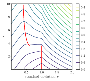
(a)

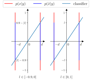
(b)

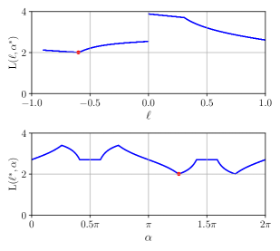
(c)

Figure 7: Visual illustrations for Lemma 1 and Lemma 2. (a) Loss contour plot for $L(v,\lambda)$ in Lemma 1. Minimizer $v^{*}(\lambda)$ is marked in red. We can see that the global minimum $v^{*}(\lambda)$ of $L(v,\lambda)$ converges to $0$ as $\lambda$ tends to infinity. (b) Setting for Lemma 2. Each sub-figure illustrates the target distribution (red), the generated distribution (blue) and the auxiliary classifier (pine). Sub-figures (from left to right) are for $\ell\in[-0.9,1]$ and $\ell\in[0,1]$, respectively. (c) Cross section plots for $L(\ell,\alpha,\lambda)$ in Lemma 2 at $\ell^{*}=-0.6,\alpha^{*}=\pi+\tan^{-1}(\tfrac{0.3}{d})\approx 1.26\pi,\lambda^{*}=2$, which is a bad critical point.

Lemma 2 (W-ACGAN with gradient descent fails to learn a separable distribution, full statement).

Consider real and fake data that are vertically uniform in $2$-dimensional space. Real data conditioned on $y\in\{\pm 1\}$ are located at ${\mathbf{x}}=({\textnormal{x}}_{1},{\textnormal{x}}_{2})=(d\cdot{\textnormal{y}},{\textnormal{u}})$ where $d=\sqrt{0.99/12}$ and ${\textnormal{u}}\sim\operatorname{Unif}[-1,1]$. Assume that the generator creates fake data from a distribution parameterized by $\ell\in[-0.9,1]$: fake data $G({\mathbf{z}},y)=(\hat{{\textnormal{x}}}_{1},\hat{{\textnormal{x}}}_{2})$ where $\hat{{\textnormal{x}}}_{1}=d\cdot y,\hat{{\textnormal{x}}}_{2}\sim\operatorname{Unif}[-\ell,\ell]$ if $\ell\in[0,1]$ and $\hat{{\textnormal{x}}}_{1}=-d\cdot y,\hat{{\textnormal{x}}}_{2}\sim\operatorname{Unif}[-(0.9-|\ell|),0.9-|\ell|]$ otherwise. An auxiliary classifier is linear that passes the origin such that $\hat{y}({\bm{x}})=\operatorname{sgn}(\tan(\alpha)x_{1}-x_{2}),\alpha\in[0,2\pi)$. The loss terms are:

$$L_{S} =\mathbb{E}_{{\textnormal{y}}}\left[W_{2}({\mathbf{x}},G({\mathbf{z}},{\textnormal{y}})))\right]$$

$$L_{C} =\mathbb{E}_{{\mathbf{x}}}\left[\bm{1}_{\{D_{\textrm{aux}}({\mathbf{x}})\neq{\textnormal{y}}\}}\right]+\mathbb{E}_{{\mathbf{z}},{\textnormal{y}}}\left[\bm{1}_{\{D_{\textrm{aux}}(G({\mathbf{z}},{\textnormal{y}}))\neq{\textnormal{y}}\}}\right],$$

Note that $L_{C}$ term indicates classification error instead of accuracy. Let $L(\ell,\alpha,\lambda)$ be $L_{S}+\lambda L_{C}$. Assume the perfect discriminator. In this setting, $L(\ell,\alpha,\lambda)$ has bad critical points, so gradient descent-based training algorithms may not converge to the global optimum.

Proof.

Recall the Wasserstein distance between two $1$-dimensional measures:

$$W_{2}({\textnormal{z}}_{1},{\textnormal{z}}_{2})=\left(\int_{0}^{1}|F_{{\textnormal{z}}_{1}}^{-1}(t)-F_{{\textnormal{z}}_{2}}^{-1}(t)|^{2}\mathop{}\!\mathrm{d}t\right)^{1/2},$$

where $F^{-1}$ is the inverse of the cumulative distribution function of a random variable. First suppose $0\leq\ell\leq 1$ so that the supports of $p_{{\mathbf{x}}|{\textnormal{y}}}({\bm{x}}|y),p_{G({\mathbf{z}},{\textnormal{y}})}({\bm{x}}|y)$ overlap. As our real and fake distributions are uniform,

$$L_{S} =\mathbb{E}_{{\textnormal{y}}}\left[W_{2}({\mathbf{x}},G({\mathbf{z}},{\textnormal{y}}))\right]=W_{2}\left(\operatorname{Unif}[-1,1],\operatorname{Unif}[-\ell,\ell]\right)$$

$$=\left(\int_{0}^{1}|(2t-1)-(2t\ell-\ell)|^{2}\mathop{}\!\mathrm{d}t\right)^{1/2}=\frac{1}{\sqrt{3}}(1-\ell)\quad\textrm{when }0\leq\ell\leq 1.$$

Suppose $-0.9\leq\ell<0$. Then, by the translation property of the Wasserstein distance, e.g., Remark 2.19 in [76],

$$\left(\mathbb{E}_{{\textnormal{y}}}\left[W_{2}({\textnormal{x}},G({\mathbf{z}},{\textnormal{y}}))\right]\right)^{2} =(2d)^{2}+W_{2}\left(\operatorname{Unif}[-1,1],\operatorname{Unif}[-(0.9-|\ell|),0.9-|\ell|]\right)^{2}$$

$$=4d^{2}+\frac{(0.1-\ell)^{2}}{3}\quad\textrm{when }-0.9\leq\ell<0.$$

Therefore, the Wasserstein distance is given by

$$L_{S}=\mathbb{E}_{{\textnormal{y}}}\left[W_{2}({\textnormal{x}},G({\mathbf{z}},{\textnormal{y}}))\right]=\sqrt{4d^{2}+\frac{(0.1-\ell)^{2}}{3}}\bm{1}_{\{-0.9\leq\ell<0\}}+\frac{1-\ell}{\sqrt{3}}\bm{1}_{\{0\leq\ell\leq 1\}}.$$

The Wasserstein distance monotonically decreases in $\ell$, so the vanilla (Wasserstein) CGAN finds $\ell^{*}=1$ by gradient descent. In this example, $d$ is chosen so that $L_{S}$ is continuous, and the mismatched range of $\ell$ is selected so that the errors of the auxiliary classifier on true data and fake data do not symmetrically move. We will see below that this solution could not be learnable by the ACGAN with gradient descent if one begins from a bad initial point.

Notice that a closed-form expression for $\mathbb{E}_{{\mathbf{x}}}\left[\bm{1}_{\{D_{\textrm{aux}}({\mathbf{x}})\neq{\textnormal{y}}\}}\right]$ in terms of $\alpha$ is given as follows. Letting $\alpha_{0}=\tan^{-1}(d^{-1})$,

$$\mathbb{E}_{{\mathbf{x}}}\left[\bm{1}_{\{D_{\textrm{aux}}({\mathbf{x}})\neq{\textnormal{y}}\}}\right]=\begin{cases}\frac{1}{2}-\frac{d\tan(\alpha)}{2}&\textrm{if }\alpha\in[2\pi-\alpha_{0},2\pi)\cup[0,\alpha_{0}]\\ 0&\textrm{if }\alpha\in(\alpha_{0},\pi-\alpha_{0})\\ \frac{1}{2}+\frac{d\tan(\alpha)}{2}&\textrm{if }\alpha\in[\pi-\alpha_{0},\pi+\alpha_{0}]\\ 1&\textrm{if }\alpha\in(\pi+\alpha_{0},2\pi-\alpha_{0}).\end{cases}$$

Let $\alpha_{+}(\ell)\coloneqq\tan^{-1}(\tfrac{\ell}{d})$ and $\alpha_{-}(\ell)\coloneqq\tan^{-1}(\tfrac{0.9-|\ell|}{d})$, we can similarly obtain a closed-form expression for $\mathbb{E}_{p_{{\mathbf{z}}}({\mathbf{z}})p_{y}(y)}\left[\bm{1}_{\{D_{\textrm{aux}}(G({\mathbf{z}},y))\neq y\}}\right]$.

$$\textrm{If }\ell\geq 0,\quad\mathbb{E}_{{\mathbf{z}},{\textnormal{y}}}\left[\bm{1}_{\{D_{\textrm{aux}}(G({\mathbf{z}},{\textnormal{y}}))\neq{\textnormal{y}}\}}\right]=\begin{cases}\frac{1}{2}-\frac{d\tan(\alpha)}{2\ell}&\textrm{if }\alpha\in[2\pi-\alpha_{+},2\pi)\cup[0,\alpha_{+}]\\ 0&\textrm{if }\alpha\in(\alpha_{+},\pi-\alpha_{+})\\ \frac{1}{2}+\frac{d\tan(\alpha)}{2\ell}&\textrm{if }\alpha\in[\pi-\alpha_{+},\pi+\alpha_{+}]\\ 1&\textrm{if }\alpha\in(\pi+\alpha_{+},2\pi-\alpha_{+}).\end{cases}$$

$$\textrm{If }\ell<0,\quad\mathbb{E}_{{\mathbf{z}},{\textnormal{y}}}\left[\bm{1}_{\{D_{\textrm{aux}}(G({\mathbf{z}},{\textnormal{y}}))\neq{\textnormal{y}}\}}\right]=\begin{cases}\frac{1}{2}+\frac{d\tan(\alpha)}{2(0.9-|\ell|)}&\textrm{if }\alpha\in[2\pi-\alpha_{-},2\pi)\cup[0,\alpha_{-}]\\ 1&\textrm{if }\alpha\in(\alpha_{-},\pi-\alpha_{-})\\ \frac{1}{2}-\frac{d\tan(\alpha)}{2(0.9-|\ell|)}&\textrm{if }\alpha\in[\pi-\alpha_{-},\pi+\alpha_{-}]\\ 0&\textrm{if }\alpha\in(\pi+\alpha_{-},2\pi-\alpha_{-}).\end{cases}$$

Let us investigate a generator obtained via alternating optimization. Fix an arbitrary $\ell^{*}<0$. Note that at $\alpha\in(\pi,\pi+\alpha_{-}(\ell^{*}))$, $\mathbb{E}_{{\mathbf{x}}}[\cdot]$ is increasing, while $\mathbb{E}_{{\mathbf{z}},{\textnormal{y}}}[\cdot]$ is decreasing faster. So $L_{C}$ is decreasing. However, as $\pi+\alpha_{-}<\pi+\alpha_{0}$, at $\alpha\in(\pi+\alpha_{-}(\ell^{*}),\pi+\alpha_{0})$, $\mathbb{E}_{{\mathbf{x}}}[\cdot]$ is increasing while $\mathbb{E}_{{\mathbf{z}},{\textnormal{y}}}[\cdot]$ is constant. So $L_{C}$ is increasing. Hence, $L_{C}$ attains its local minimum $\alpha^{*}=\pi+\alpha_{-}(\ell^{*})$ by gradient descent.

Now fix $\alpha^{*}=\pi+\alpha_{-}(\ell^{*})$. As $\mathbb{E}_{{\mathbf{z}},{\textnormal{y}}}[\cdot]$ is decreasing on $\ell<\ell^{*}$ and increasing on $\ell>\ell^{*}$, while $\mathbb{E}_{{\mathbf{x}}}[\cdot]$ remains unchanged. So $L_{C}$ term has its local minimum at $\ell^{*}$ for a given $\alpha^{*}$. Note that $L_{S}$ is decreasing in $\ell$. Hence by picking large $\lambda^{*}$ such that $L_{C}$ term dominates $L_{S}$, the generator learns $\ell^{*}\neq 1$ by gradient method. Fig. 7(c) depicts the cross-section of $L(\ell,\alpha,\lambda)$ at $\ell^{*}=-0.6$, $\alpha^{*}=\pi+\tan(\tfrac{0.3}{d})\approx 1.26\pi$, $\lambda^{*}=2$ and demonstrates this is a bad critical point. ∎

A.1.2 Examples of the failure of ProjGAN

We provide an example to show why and when ProjGAN [2] may fail to work. Note that the ProjGAN’s discriminator takes an inner product between a feature vector and the class embedded vector, that is,

$$D({\bm{x}},{\bm{y}};{\bm{\theta}}_{D})={\bm{y}}^{T}{\bm{V}}\phi({\bm{x}})+\psi(\phi({\bm{x}})),$$

where ${\bm{y}}$ is an one-hot encoded label vector, ${\bm{V}}=[{\bm{v}}_{1}^{T};{\bm{v}}_{2}^{T};\cdots]$ is the label embedding matrix of ${\mathbf{y}}$, and $\phi$, $\psi$ are learnable functions. This special algebraic operation reduces to expectation matching in a simple setting, by which we can provably show that ProjGAN mislearns the exact conditional distributions.

Lemma 3 (full statement).

Assume $\phi({\bm{x}})={\bm{x}}$ and $\psi({\bm{x}})=0$ for an equiprobable two-class data. Thus, ${\bm{\theta}}_{D}=\{{\bm{V}}\}$ with ${\bm{V}}=\begin{bmatrix}{\bm{v}}_{0}^{T}\\ {\bm{v}}_{1}^{T}\end{bmatrix}$. With hinge loss, the loss for the discriminator to minimize is written as

$$L_{D} =\mathbb{E}_{{\mathbf{x}},{\textnormal{y}}}\left[\max(0,1-D({\mathbf{x}},{\textnormal{y}};{\bm{\theta}}_{D}))\right]+\mathbb{E}_{{\mathbf{z}},{\textnormal{y}}}\left[\max(0,1+D(G({\mathbf{z}},{\textnormal{y}}),{\textnormal{y}};{\bm{\theta}}_{D}))\right].$$

Let us further suppose that the generator learned the exact conditional distributions at time $t^{*}$, that is, $G_{t^{*}}({\mathbf{z}},y)\sim{\mathbf{x}}|{\textnormal{y}}=y$, where $G_{t}$ stands for the generator at time $t$. Then, there exist discriminator’s bad embedding vectors that encourage the generator to deviate from the exact conditional distributions.

Proof.

Note that the discriminator $D$ under the setting is

$$\begin{split}D({\bm{x}},{\bm{y}};{\bm{\theta}}_{D})&={\bm{y}}^{T}{\bm{V}}\phi({\bm{x}})+\psi(\phi({\bm{x}}))\\ &={\bm{y}}^{T}{\bm{V}}{\bm{x}}.\end{split}$$ (3)

With hinge loss, the loss for the discriminator to minimize is written as

$$L_{D}=\mathbb{E}_{{\mathbf{x}},{\textnormal{y}}}\left[\max(0,1-D({\mathbf{x}},{\textnormal{y}};{\bm{\theta}}_{D}))\right]+\mathbb{E}_{{\mathbf{z}},{\textnormal{y}}}\left[\max(0,1+D(G({\mathbf{z}},{\textnormal{y}}),{\textnormal{y}};{\bm{\theta}}_{D}))\right].$$

For simple presentation, we restrict ranges of ${\mathbf{x}},{\bm{v}}_{y}$ properly so that $D={\bm{y}}^{T}{\bm{V}}{\bm{x}}$ is in $(-1,1)$. Then, we can omit the $\max$ operator. As classes are equally likely and our setting assumes $D={\bm{y}}^{T}{\bm{V}}{\bm{x}}$,

$$L_{D} =\frac{1}{2}(\mathbb{E}_{p_{\text{data}}({\bm{x}}|y=0)}\left[1-D({\mathbf{x}},0;{\bm{\theta}}_{D})\right]$$

$$+\mathbb{E}_{p_{\text{data}}({\bm{x}}|y=1)}\left[1-D({\mathbf{x}},1;{\bm{\theta}}_{D})\right]+\mathbb{E}_{{\mathbf{z}},{\textnormal{y}}=0}\left[1+D(G({\mathbf{z}},0),0;{\bm{\theta}}_{D})\right]+\mathbb{E}_{{\mathbf{z}},{\textnormal{y}}=1}\left[1+D(G({\mathbf{z}},1),1;{\bm{\theta}}_{D})\right])$$

$$=\frac{1}{2}\mathbb{E}_{p_{\text{data}}({\bm{x}}|y=0)}\left[1-{\bm{v}}_{0}^{T}{\mathbf{x}}\right]+\frac{1}{2}\mathbb{E}_{p_{\text{data}}({\bm{x}}|y=1)}\left[1-{\bm{v}}_{1}^{T}{\mathbf{x}}\right]+\frac{1}{2}\mathbb{E}_{{\mathbf{z}},{\textnormal{y}}=0}\left[1+{\bm{v}}_{0}^{T}G({\mathbf{z}},0)\right]+\frac{1}{2}\mathbb{E}_{{\mathbf{z}},{\textnormal{y}}=1}\left[1+{\bm{v}}_{1}^{T}G({\mathbf{z}},1)\right].$$

Hence, the gradient is in a simple form:

$$\nabla_{{\bm{v}}_{y}}L_{D}=-\frac{1}{2}\mathbb{E}_{p_{\text{data}}({\bm{x}}|y)}[{\mathbf{x}}]+\frac{1}{2}\mathbb{E}_{{\mathbf{z}},{\textnormal{y}}=y}[G({\mathbf{z}},y)],$$ (4)

which means that the discriminator measures the difference between conditional means of true data and generated data.

Note that the loss for the generator to minimize is

$$L_{G} =-\mathbb{E}_{{\mathbf{z}},{\textnormal{y}}=0}[D(G({\mathbf{z}},0),0;{\bm{\theta}}_{D})]-\mathbb{E}_{{\mathbf{z}},{\textnormal{y}}=1}[D(G({\mathbf{z}},1),1;{\bm{\theta}}_{D})]$$

$$=-\mathbb{E}_{{\mathbf{z}},{\textnormal{y}}=0}[{\bm{v}}_{0}^{T}G({\mathbf{z}},0)]-\mathbb{E}_{{\mathbf{z}},{\textnormal{y}}=1}[{\bm{v}}_{1}^{T}G({\mathbf{z}},1)].\vspace{-5mm}$$

Its gradient is also in a simple form:

$$\nabla_{G}L_{G}=-{\bm{v}}_{0}-{\bm{v}}_{1}.$$ (5)

Now we are ready to discuss why ProjGAN may fail to learn correct distributions. Let us suppose that the generator learned the exact conditional distributions at time $t^{*}$, that is, $G_{t^{*}}({\mathbf{z}},y)\sim{\mathbf{x}}|{\textnormal{y}}=y$. This in turn implies $\mathbb{E}_{p_{\text{data}}({\bm{x}}|y)}[{\mathbf{x}}]=\mathbb{E}_{{\mathbf{z}},{\textnormal{y}}=y}[G_{t^{*}}({\mathbf{z}},y)]$ for $y=0,1$. Note that (4), (5) yield the following update:

$$G_{t+1}({\mathbf{z}},y) =G_{t}({\mathbf{z}},y)-\eta\nabla_{G}L_{G}=G_{t}({\mathbf{z}},y)+\alpha({\bm{v}}_{0,t}+{\bm{v}}_{1,t})$$

$${\bm{v}}_{y,t+1} ={\bm{v}}_{y,t}-\eta\nabla_{{\bm{v}}_{y}}L_{D}={\bm{v}}_{y,t}+\frac{\alpha}{2}\left(\mathbb{E}_{p_{\text{data}}({\bm{x}}|y)}[{\mathbf{x}}]-\mathbb{E}_{{\mathbf{z}},{\textnormal{y}}=y}[G_{t}({\mathbf{z}},y)]\right).$$

Therefore, assuming that the step size $\alpha$ is small, alternating update yields the following dynamics after $t^{*}$.

First update:

$$G({\mathbf{z}},y) \leftarrow G_{t^{*}}({\mathbf{z}},y)+\alpha({\bm{v}}_{0,t^{*}}+{\bm{v}}_{1,t^{*}})$$

$${\bm{v}}_{y} \leftarrow{\bm{v}}_{y,t^{*}}+\frac{\alpha}{2}\left(\mathbb{E}_{p_{\text{data}}({\bm{x}}|y)}[{\mathbf{x}}]-\mathbb{E}_{{\mathbf{z}},{\textnormal{y}}=y}[G({\mathbf{z}},y)]\right)$$

$$={\bm{v}}_{y,t^{*}}+\frac{\alpha}{2}\left(\mathbb{E}_{p_{\text{data}}({\bm{x}}|y)}[{\mathbf{x}}]-\mathbb{E}_{{\mathbf{z}},{\textnormal{y}}=y}\left[G_{t^{*}}+\alpha({\bm{v}}_{0,t^{*}}+{\bm{v}}_{1,t^{*}})\right]\right)$$

$$={\bm{v}}_{y,t^{*}}-\frac{\alpha^{2}}{2}({\bm{v}}_{0,t^{*}}+{\bm{v}}_{1,t^{*}})~{}~{}~{}\textrm{since the conditional first moments are the same}$$

Second update:

$$G({\mathbf{z}},y) \leftarrow G({\mathbf{z}},y)+\alpha({\bm{v}}_{0}+{\bm{v}}_{1})$$

$$=\left(G_{t^{*}}({\mathbf{z}},y)+\alpha({\bm{v}}_{0,t^{*}}+{\bm{v}}_{1,t^{*}})\right)+\alpha\left({\bm{v}}_{0,t^{*}}-\frac{\alpha^{2}}{2}({\bm{v}}_{0,t^{*}}+{\bm{v}}_{1,t^{*}})+{\bm{v}}_{1,t^{*}}-\frac{\alpha^{2}}{2}({\bm{v}}_{0,t^{*}}+{\bm{v}}_{1,t^{*}})\right)$$

$$=G_{t^{*}}({\mathbf{z}},y)+2\alpha({\bm{v}}_{0,t^{*}}+{\bm{v}}_{1,t^{*}})-\alpha^{2}({\bm{v}}_{0,t^{*}}+{\bm{v}}_{1,t^{*}})$$

$$\approx G_{t^{*}}({\mathbf{z}},y)+2\alpha({\bm{v}}_{0,t^{*}}+{\bm{v}}_{1,t^{*}})~{}~{}~{}\textrm{since $\alpha$ is small}$$

$${\bm{v}}_{y} \leftarrow{\bm{v}}_{y}+\frac{\alpha}{2}(-2\alpha({\bm{v}}_{0,t^{*}}+{\bm{v}}_{1,t^{*}}))~{}~{}~{}\textrm{since the difference between first moments is zero at $t$}$$

$$=\left({\bm{v}}_{y,t^{*}}-\frac{\alpha^{2}}{2}({\bm{v}}_{0,t^{*}}+{\bm{v}}_{1,t^{*}})\right)+\frac{\alpha}{2}\left(-2\alpha({\bm{v}}_{0,t^{*}}+{\bm{v}}_{1,t^{*}})\right)$$

$$={\bm{v}}_{y,t^{*}}-\frac{3\alpha^{2}}{2}({\bm{v}}_{0,t^{*}}+{\bm{v}}_{1,t^{*}})$$

Third update:

$$G({\mathbf{z}},y) \leftarrow G({\mathbf{z}},y)+\alpha({\bm{v}}_{0}+{\bm{v}}_{1})$$

$$=\left(G_{t^{*}}({\mathbf{z}},y)+2\alpha({\bm{v}}_{0,t^{*}}+{\bm{v}}_{1,t^{*}})\right)+\alpha\left({\bm{v}}_{0,t^{*}}-\frac{3\alpha^{2}}{2}({\bm{v}}_{0,t^{*}}+{\bm{v}}_{1,t^{*}})+{\bm{v}}_{1,t^{*}}-\frac{3\alpha^{2}}{2}({\bm{v}}_{0,t^{*}}+{\bm{v}}_{1,t^{*}})\right)$$

$$\approx G_{t^{*}}({\mathbf{z}},y)+3\alpha({\bm{v}}_{0,t^{*}}+{\bm{v}}_{1,t^{*}})~{}~{}~{}\textrm{since $\alpha$ is small}$$

$${\bm{v}}_{y} \leftarrow{\bm{v}}_{y}+\frac{\alpha}{2}(-3\alpha({\bm{v}}_{0,t^{*}}+{\bm{v}}_{1,t^{*}}))$$

$$={\bm{v}}_{y,t^{*}}-3\alpha^{2}({\bm{v}}_{0,t^{*}}+{\bm{v}}_{1,t^{*}}).$$

Repeating the updates, the $G({\mathbf{z}},y)$ steadily diverges from $G_{t^{*}}$ unless ${\bm{v}}_{0,t^{*}}+{\bm{v}}_{1,t^{*}}=0$. In other words, even when the generator exactly learns the true data at time $t^{*}$, nonvanishing $\nabla_{G}L_{G}$ may result in the divergence of the generator. ∎

A.2 Full statements and proofs for Section 3.1

We provide the following proposition to justify the use of reprogramming for GAN conditioning. This proposition implies that, given an unconditional generator learned on $p_{\text{data}}({\bm{x}})$, one can take condition-specific noise ${\mathbf{z}}_{y}$ to generate data from the target conditional distribution $p_{\text{data}}({\bm{x}}|y)$.

Proposition 2 (full statement).

Assume that for two random variables ${\mathbf{z}}$ and ${\mathbf{x}}$ having continuous probability density functions, we have a perfect continuous generator $G:{\mathbb{Z}}\mapsto{\mathbb{X}}$ that satisfies the following: (i) $G({\mathbf{z}})\,{=_{d}}\,{\mathbf{x}}$, (ii) $G^{-1}({\bm{x}})$ is Lipschitz continuous around each ${\bm{z}}_{i}\in G^{-1}({\bm{x}})$, and (iii) the Jacobian of $G$ has finite operator norm. In addition, assume that $p_{{\textnormal{y}}|{\mathbf{x}}}(y|{\bm{x}})$ is continuous in ${\bm{x}}$ for all $y\in{\mathbb{Y}}$. Then, for any discrete random variable y, possibly dependent on ${\mathbf{x}}$, we can construct a random variable ${\mathbf{z}}_{y}$ such that $G({\mathbf{z}}_{y})\,{=_{d}}\,{\mathbf{x}}|{\textnormal{y}}=y$.

Proof.

Fix $y$ and take ${\mathbf{z}}_{y}$ as follows:

$$p_{{\mathbf{z}}_{y}}({\bm{z}})=p_{{\mathbf{z}}}({\bm{z}})\cdot\frac{p_{{\textnormal{y}}|{\mathbf{x}}}(y|G({\bm{z}}))}{p_{{\textnormal{y}}}(y)}.$$

Let $B({\bm{x}}_{0},r)\subset{\mathbb{X}}$ be a small ball of radius $r$ centered at ${\bm{x}}_{0}$. Since ${\mathbf{x}}$ has a continuous density function, we know that every ${\bm{x}}$ is a Lebesgue point [77], which implies that

$$\frac{p_{\mathbf{x}}(B)}{\mu(B)}\to p_{\mathbf{x}}({\bm{x}}_{0})~{}~{}~{}\textrm{as $r\to 0$},$$ (6)

where $\mu(\cdot)$ is the Lebesgue measure.

On the other hand, as $G^{-1}$ could have finite (say at most $T$) multiple images, let

$$G^{-1}(B)=\Omega_{1}\cup\cdots\cup\Omega_{t},~{}~{}t\leq T,$$

where $\Omega_{i}$ are disjoint each other.

With the above construction, we have the following.

$$p_{{\mathbf{x}}}(G({\bm{z}}_{y})\in B) =p_{{\mathbf{z}}_{y}}({\bm{z}}_{y}\in G^{-1}(B))=p_{{\mathbf{z}}_{y}}\left({\bm{z}}_{y}\in\sum_{i=1}^{t}\Omega_{i}\right)=\sum_{i=1}^{t}p_{{\mathbf{z}}_{y}}\left({\bm{z}}_{y}\in\Omega_{i}\right).$$

Then for each $i$, we can bound the probability as follows: Letting $z_{0}=G^{-1}({\bm{x}}_{0})$ in $\Omega_{i}$,

$$\int_{\Omega_{i}}p_{{\mathbf{z}}_{y}}({\bm{z}})\mathop{}\!\mathrm{d}{\bm{z}}=\int_{\Omega_{i}}p_{{\mathbf{z}}}({\bm{z}})\frac{p_{{\textnormal{y}}|{\mathbf{x}}}(y|G({\bm{z}}))}{p_{{\textnormal{y}}}(y)}\mathop{}\!\mathrm{d}{\bm{z}}$$

$$\stackrel{{\scriptstyle(a)}}{{=}}\int_{\Omega_{i}}p_{{\mathbf{z}}}({\bm{z}})\left(\frac{p_{{\textnormal{y}}|{\mathbf{x}}}(y|{\bm{x}}_{0})}{p_{{\textnormal{y}}}(y)}+h_{i}({\bm{z}}-{\bm{z}}_{0})\right)\mathop{}\!\mathrm{d}{\bm{z}}$$

$$=p_{{\mathbf{z}}}(\Omega_{i})\frac{p_{{\textnormal{y}}|{\mathbf{x}}}(y|{\bm{x}}_{0})}{p_{{\textnormal{y}}}(y)}+\int_{\Omega_{i}}p_{{\mathbf{z}}}({\bm{z}})h_{i}({\bm{z}}-{\bm{z}}_{0})\mathop{}\!\mathrm{d}{\bm{z}}$$ (7)

where (a) follows from the Taylor series with remainders being $h_{i}({\bm{z}}-{\bm{z}}_{0})$.

Let us consider the second term. Because $G^{-1}$ is Lipschitz on $\Omega_{i}$, we can take a small ball $A({\bm{z}}_{0},Kr)$ such that $\Omega_{i}\subset A({\bm{z}}_{0},Kr)$ where $A({\bm{z}}_{0},Kr)$ is the sphere centered at ${\bm{z}}_{0}$ and of radius $Kr$ with the Lipschitz constant of $G^{-1}$ being $K$. Ignoring high-order terms of $h(\cdot)$ that are asymptotically negligible, the second term can be rewritten with the linear term only. Letting $\bm{g}$ be the Jacobian of $\tfrac{p_{{\textnormal{y}}|{\mathbf{x}}}(y|G({\bm{z}}))}{p_{{\textnormal{y}}}(y)}$ at ${\bm{z}}_{0}$,

$$\int_{\Omega_{i}}p_{{\mathbf{z}}}({\bm{z}})h({\bm{z}}-{\bm{z}}_{0})\mathop{}\!\mathrm{d}{\bm{z}} \approx\int_{\Omega_{i}}p_{{\mathbf{z}}}({\bm{z}})\bm{g}({\bm{z}}-{\bm{z}}_{0})\mathop{}\!\mathrm{d}{\bm{z}}$$

$$\stackrel{{\scriptstyle(b)}}{{\leq}}\textrm{const}\cdot\int_{\Omega_{i}}\bm{g}({\bm{z}}-{\bm{z}}_{0})\mathop{}\!\mathrm{d}{\bm{z}}\leq\textrm{const}\cdot\int_{\Omega_{i}}\left|\bm{g}({\bm{z}}-{\bm{z}}_{0})\right|\mathop{}\!\mathrm{d}{\bm{z}}$$

$$\stackrel{{\scriptstyle(c)}}{{\leq}}\textrm{const}\cdot\int_{A({\bm{z}}_{0},Kr)}\left|\bm{g}({\bm{z}}-{\bm{z}}_{0})\right|\mathop{}\!\mathrm{d}{\bm{z}}\leq\textrm{const}\cdot\int_{A({\bm{z}}_{0},Kr)}\|\bm{g}\|\cdot\|{\bm{z}}-{\bm{z}}_{0}\|\mathop{}\!\mathrm{d}{\bm{z}}$$

$$\stackrel{{\scriptstyle(d)}}{{\leq}}\textrm{const}\cdot\int_{A({\bm{z}}_{0},Kr)}\|{\bm{z}}-{\bm{z}}_{0}\|\mathop{}\!\mathrm{d}{\bm{z}}$$

where (b) follows since $p_{{\mathbf{z}}}({\bm{z}})$ is bounded on a compact set, (c) follows since $\Omega_{i}\subset A({\bm{z}}_{0},Kr)$, and (d) follows since the Jacobian has finite operator norm. The final bound is computable in closed form using polar coordinates [78],

$$\int_{\Omega_{i}}p_{{\mathbf{z}}}({\bm{z}})h_{i}({\bm{z}}-{\bm{z}}_{0})\mathop{}\!\mathrm{d}{\bm{z}} \leq\textrm{const}\cdot\int_{A({\bm{z}}_{0},Kr)}\|{\bm{z}}-{\bm{z}}_{0}\|\mathop{}\!\mathrm{d}{\bm{z}}$$

$$=\textrm{const}\cdot S^{d-1}\int_{0}^{Kr}\rho\cdot\rho^{d-1}\mathop{}\!\mathrm{d}\rho$$

$$=\textrm{const}\cdot S^{d-1}\frac{(Kr)^{d+1}}{d+1}$$

$$=\textrm{const}\cdot r^{d+1},$$

where $S^{d-1}$ is the surface area of the unit sphere in $\mathbb{R}^{d}$. Substituting this into ( 7), we have the following.

$$p_{{\mathbf{x}}}(G({\bm{z}}_{y})\in B) =\sum_{i=1}^{t}p_{{\mathbf{z}}_{y}}\left({\bm{z}}_{y}\in\Omega_{i}\right)$$

$$\leq p_{\mathbf{x}}(B)\frac{p_{{\textnormal{y}}|{\mathbf{x}}}(y|{\bm{x}}_{0})}{p_{{\textnormal{y}}}(y)}+\sum_{i=1}^{t}\textrm{const}\cdot r^{d+1}$$

$$\leq p_{\mathbf{x}}(B)\frac{p_{{\textnormal{y}}|{\mathbf{x}}}(y|{\bm{x}}_{0})}{p_{{\textnormal{y}}}(y)}+\textrm{const}T\cdot r^{d+1}.$$

Normalizing both sides by the volume of $B$, $\mu(B)=\textrm{const}\cdot r^{d}$, and taking $r\to 0$, the property of Lebesgue points (6) concludes that

$$\frac{p_{{\mathbf{x}}}(G({\mathbf{z}}_{y})\in B)}{\mu(B)}=\frac{p_{\mathbf{x}}(B)}{\mu(B)}\frac{p_{{\textnormal{y}}|{\mathbf{x}}}(y|{\bm{x}}_{0})}{p_{{\textnormal{y}}}(y)}+\textrm{const}\cdot r$$

$$\implies p_{{\mathbf{x}}}(G({\mathbf{z}}_{y})={\bm{x}}_{0})\to\frac{p_{{\mathbf{x}}}({\bm{x}}_{0})p_{{\textnormal{y}}|{\mathbf{x}}}(y|{\bm{x}}_{0})}{p_{{\textnormal{y}}}(y)}=p_{{\mathbf{x}}|{\textnormal{y}}}({\bm{x}}_{0}|y)~{}~{}\textrm{as $r\to 0$}.$$

Since the argument holds for arbitrary ${\bm{x}}_{0}$, $G({\mathbf{z}}_{y})\,{=_{d}}\,{\mathbf{x}}|{\bm{y}}=y$. ∎

A.3 Full statements and proofs for Section 3.3

We need one simple proposition before showing the theorem.

Proposition 1 (restatement).

When the ideal unconditional generator $G$ and arbitrary modifier $M_{y}$ are fixed, the optimal discriminator for $y$ is

$$D_{y}^{*}(M_{y}({\bm{u}}))=\frac{(1+\pi_{y})p_{\text{data}}({\bm{x}}|y)}{(1+\pi_{y})p_{\text{data}}({\bm{x}}|y)+(1-\pi_{y})p_{\text{gf}}({\bm{x}})}.$$

Proof.

Using $p_{G(M_{y}({\mathbf{u}}))}({\bm{x}})=\pi_{y}p_{\text{data}}({\bm{x}}|y)+(1-\pi_{y})p_{\text{gf}}({\bm{x}})$, we can rewrite $V_{y}^{PU}$.

$$V_{y}^{PU}={} (1+\pi_{y})\mathbb{E}_{{\mathbf{x}}\sim p_{\text{data}}({\bm{x}}|y)}[\log D_{y}({\mathbf{x}})]+\mathbb{E}_{{\mathbf{x}}\sim p_{G(M_{y}({\mathbf{u}}))}({\bm{x}})}[\log(1-D_{y}({\mathbf{x}}))]-\pi_{y}\mathbb{E}_{{\mathbf{x}}\sim p_{\text{data}}({\bm{x}}|y)}[\log(1-D_{y}({\mathbf{x}}))]$$

$$\begin{split}={}&\int_{{\bm{x}}}\Big{[}(1+\pi_{y})p_{\text{data}}({\bm{x}}|y)\log D_{y}({\bm{x}})+\left(\pi_{y}p_{\text{data}}({\bm{x}}|y)+(1-\pi_{y})p_{\text{gf}}({\bm{x}})\right)\log(1-D_{y}({\bm{x}}))\\ &-\pi_{y}p_{\text{data}}({\bm{x}}|y)\log(1-D_{y}({\bm{x}}))\Big{]}\mathop{}\!\mathrm{d}{\bm{x}}\end{split}$$

$$={} \int_{{\bm{x}}}(1+\pi_{y})p_{\text{data}}({\bm{x}}|y)\log D_{y}({\bm{x}})+(1-\pi_{y})p_{\text{gf}}({\bm{x}})\log(1-D_{y}({\bm{x}}))\mathop{}\!\mathrm{d}{\bm{x}}.$$

Since $\int a\log y+b\log(1-y)$ attains its maximum at $y^{*}=\frac{a}{a+b}$, we can conclude that

$$D_{y}^{*}(M_{y}({\bm{u}}))=\frac{(1+\pi_{y})p_{\text{data}}({\bm{x}}|y)}{(1+\pi_{y})p_{\text{data}}({\bm{x}}|y)+(1-\pi_{y})p_{\text{gf}}({\bm{x}})}.$$

∎

Theorem 1 (full statement).

When the ideal unconditional generator $G^{*}$ and discriminator $D^{*}$ are fixed, the global optimal modifier $M_{y}$ is attained if and only if $p_{\text{gf}}({\bm{x}})=p_{g}({\bm{x}})=p_{\text{data}}({\bm{x}}|y)$. Moreover, the loss achieved at $p_{g}({\bm{x}})=p_{\text{data}}({\bm{x}}|y)$ is $(1+\pi_{y})\log\tfrac{(1+\pi_{y})}{2}+(1-\pi_{y})\log\tfrac{(1-\pi_{y})}{2}$.

Proof.

Note that $((1+\pi_{y})p_{\text{data}}+(1-\pi)p_{\text{gf}})/2$ is a valid probability distribution. Since $D_{y}^{*}$ in Proposition 2 is fixed,

$$\begin{split}V_{y}^{PU}={}&\int_{{\bm{x}}}\Big{[}(1+\pi_{y})p_{\text{data}}({\bm{x}}|{\textnormal{y}}=y)\log\frac{(1+\pi_{y})p_{\text{data}}({\bm{x}}|{\textnormal{y}}=y)}{(1+\pi_{y})p_{\text{data}}({\bm{x}}|{\textnormal{y}}=y)+(1-\pi_{y})p_{\text{gf}}}\\ &+(1-\pi_{y})p_{\text{gf}}\log\frac{(1-\pi_{y})p_{\text{gf}}}{(1+\pi_{y})p_{\text{data}}({\bm{x}}|{\textnormal{y}}=y)+(1-\pi_{y})p_{\text{gf}}}\Big{]}\mathop{}\!\mathrm{d}{\bm{x}}\end{split}$$

$$\begin{split}={}&(1+\pi_{y})\int_{{\bm{x}}}p_{\text{data}}({\bm{x}}|{\textnormal{y}}=y)\log\left(\frac{p_{\text{data}}({\bm{x}}|{\textnormal{y}}=y)}{((1+\pi_{y})p_{\text{data}}({\bm{x}}|{\textnormal{y}}=y)+(1-\pi_{y})p_{\text{gf}})/2}\cdot\frac{1+\pi_{y}}{2}\right)\mathop{}\!\mathrm{d}{\bm{x}}\\ &+(1-\pi_{y})\int_{{\bm{x}}}p_{\text{gf}}\log\left(\frac{p_{\text{gf}}}{((1+\pi_{y})p_{\text{data}}({\bm{x}}|{\textnormal{y}}=y)+(1-\pi_{y})p_{\text{gf}})/2}\cdot\frac{1-\pi_{y}}{2}\right)\mathop{}\!\mathrm{d}{\bm{x}}\end{split}$$

$$\begin{split}={}&(1+\pi_{y})\mathrm{KL}\left(p_{\text{data}}({\bm{x}}|{\textnormal{y}}=y)\middle\|\frac{p_{\text{data}}({\bm{x}}|{\textnormal{y}}=y)}{((1+\pi_{y})p_{\text{data}}({\bm{x}}|{\textnormal{y}}=y)+(1-\pi_{y})p_{\text{gf}})/2}\right)+(1+\pi_{y})\log\frac{1+\pi_{y}}{2}\\ &+(1-\pi_{y})\mathrm{KL}\left(p_{\text{gf}}\middle\|\frac{p_{\text{data}}({\bm{x}}|{\textnormal{y}}=y)}{((1+\pi_{y})p_{\text{data}}({\bm{x}}|{\textnormal{y}}=y)+(1-\pi_{y})p_{\text{gf}})/2}\right)+(1-\pi_{y})\log\frac{1-\pi_{y}}{2},\end{split}$$

where $\mathrm{KL}(\cdot\|\cdot)$ is the Kullback–Leibler divergence. Optimizing $M_{y}$ yields the global optimum $p_{\text{gf}}({\bm{x}})=p_{\text{data}}({\bm{x}}|y)$ and therefore, $p_{\text{gf}}({\bm{x}})=p_{\text{data}}({\bm{x}}|y)=p_{G(M_{y}({\mathbf{u}}))}({\bm{x}})$. ∎

Appendix B Details of Experiment Settings and Implementation

B.1 Datasets

MNIST [79] contains ten classes of $28\times 28$ black-and-white images, with $50\,000$ training images and $10\,000$ testing images. CIFAR10 [54] dataset is a widely used benchmark dataset in image synthesis. The dataset contains ten classes of three-channel (color) $32\times 32$ pixel images, with $50\,000$ training and $10\,000$ testing images. CIFAR100 [54] contains 100 classes of three-channel (color) $32\times 32$ pixel images (similar to CIFAR10 images). Each class contains 600 images: 500 images for training and 100 images for testing. CelebA [56] is a large-scale dataset of celebrity face that has more than $200\,000$ images with 40 attributes for each image. Flickr-Faces-HQ (FFHQ) [55] is the dataset of human faces, which consists of $70\,000$ high-quality images at $1024\times 1024$ resolution, crawled from Flickr.

B.2 Evaluation metrics

Frechet Inception Distance (FID) is a widely-used metric to measure the quality and diversity of learned distributions in the GAN literature. FID is Wasserstein-2 (Fréchet) distance between Gaussians fitted to the data embedded into the feature space of the Inception-v3 model (pool3 activation layer). Lower FID indicates better GAN’s performance. As FID relies on a feature space from a classifier trained on ImageNet, FID is not suitable for non-ImageNet-like images (e.g., MNIST or Fashion-MNIST). For conditional GANs, we also calculate the FID for each particular class data and get the average score as Intra-FID score [2]. This score measures class-conditioning performances.

Classification Accuracy Score (CAS) [59] measures the accuracy of a classifier trained with the generated conditional data. More specifically, we train a classifier using labeled data generated by conditional generators and measure the classification accuracy of the trained classifier on the real dataset as CAS. Intuitively, if the generated distribution matches the real distribution, CAS should be close to the accuracy of the classifier trained on real samples.

Recall [58] measures how well the learned distribution covers the true (or reference) distribution. The value of the recall score is between $0$ and $1$. Higher recall scores indicate better coverage.

B.3 Architectures, hyperparameters, and implementation

Our goal is to compare the effectiveness of InRep+ with other methods, rather than to produce the model with the state-of-the-art performance on data synthesis. The latter part usually requires much more computations and tricks. Therefore, we conduct fair and reliable assessments of conditioning methods on widely used GANs. We apply the same configuration for all models.

We use different configurations for different datasets. For the Gaussian mixture, we use a simple network architecture with three blocks. Each block consists of a fully connected layer followed by a batch-normalization and a ReLU activation function. We use non-saturating GAN loss [1]. We train each model with $10\,000$ steps (batch size of $64$), using Adam Optimizer ($\beta_{1}=0.5,\beta_{2}=0.999$) with learning rate $2\cdot 10^{-4}$ for all networks. For MNIST, We adopt WGAN-GP [14] with DCGAN architectures for MNIST [80]. The loss is Wasserstein loss with gradient penalty regularization. We set the number of critic steps to be five. We train each model $50\,000$ steps (batch size of 64) using Adam Optimizer ($\beta_{1}=0.5,\beta_{2}=0.999$) with learning rates $2\cdot 10^{-4},2\cdot 10^{-5}$ for modifier and discriminator networks, respectively. On CIFAR10 and CIFAR100, among three widely used architectures in the GAN literature (DCGAN, ResGAN, and BigGAN), we adopt ResGAN for all models given that [62] observes the comparable performance between DCGAN and ResGAN on various settings of GANs. Also, we apply best practices and recommended configurations for each model [62, 3]: spectral normalization (an essential element in modern GAN training), Hinge loss [81]. For InRep+, the modifier network adopts the architecture of i-ResNet [31], with five layers for FFHQ data and three layers for CIFAR datasets.

References

- [1] Ian Goodfellow, Jean Pouget-Abadie, Mehdi Mirza, Bing Xu, David Warde-Farley, Sherjil Ozair, Aaron Courville, and Yoshua Bengio. Generative adversarial nets. In Advances in Neural Information Processing Systems (NIPS), 2014.
- [2] Takeru Miyato and Masanori Koyama. cGANs with projection discriminator. In International Conference on Learning Representations (ICLR), 2018.
- [3] Mario Lučić, Michael Tschannen, Marvin Ritter, Xiaohua Zhai, Olivier Bachem, and Sylvain Gelly. High-fidelity image generation with fewer labels. In International Conference on Machine Learning (ICML), 2019.
- [4] Minguk Kang and Jaesik Park. ContraGAN: Contrastive learning for conditional image generation. In Advances in Neural Information Processing Systems (NeurIPS), 2020.
- [5] Phillip Isola, Jun-Yan Zhu, Tinghui Zhou, and Alexei A Efros. Image-to-image translation with conditional adversarial networks. In IEEE/CVF Conference on Computer Vision and Pattern Recognition (CVPR), 2017.
- [6] Jun-Yan Zhu, Taesung Park, Phillip Isola, and Alexei A Efros. Unpaired image-to-image translation using cycle-consistent adversarial networks. In IEEE/CVF International Conference on Computer Vision (ICCV), 2017.
- [7] Lantao Yu, Weinan Zhang, Jun Wang, and Yong Yu. SeqGAN: Sequence generative adversarial nets with policy gradient. In AAAI Conference on Artificial Intelligence (AAAI), 2017.
- [8] Jiaxian Guo, Sidi Lu, Han Cai, Weinan Zhang, Yong Yu, and Jun Wang. Long text generation via adversarial training with leaked information. In AAAI Conference on Artificial Intelligence (AAAI), 2018.
- [9] Haoye Dong, Xiaodan Liang, Xiaohui Shen, Bowen Wu, Bing-Cheng Chen, and Jian Yin. FW-GAN: Flow-navigated warping gan for video virtual try-on. In IEEE/CVF International Conference on Computer Vision (ICCV), 2019.
- [10] Soo Ye Kim, Jihyong Oh, and Munchurl Kim. JSI-GAN: GAN-based joint super-resolution and inverse tone-mapping with pixel-wise task-specific filters for uhd hdr video. In AAAI Conference on Artificial Intelligence (AAAI), 2020.
- [11] Jungil Kong, Jaehyeon Kim, and Jaekyoung Bae. HiFi-GAN: Generative adversarial networks for efficient and high fidelity speech synthesis. arXiv preprint arXiv:2010.05646, 2020.
- [12] Tom B Brown, Benjamin Mann, Nick Ryder, Melanie Subbiah, Jared Kaplan, Prafulla Dhariwal, Arvind Neelakantan, Pranav Shyam, Girish Sastry, Amanda Askell, et al. Language models are few-shot learners. arXiv preprint arXiv:2005.14165, 2020.
- [13] Su Lin Blodgett, Solon Barocas, Hal Daumé III, and Hanna Wallach. Language (technology) is power: A critical survey of "bias" in NLP. arXiv preprint arXiv:2005.14050, 2020.
- [14] Martin Arjovsky, Soumith Chintala, and Leon Bottou. Wasserstein generative adversarial networks. In International Conference on Machine Learning (ICML), 2017.
- [15] Takeru Miyato, Toshiki Kataoka, Masanori Koyama, and Yuichi Yoshida. Spectral normalization for generative adversarial networks. In International Conference on Learning Representations (ICLR), 2018.
- [16] https://github.com/ajbrock/BigGAN-PyTorch, accessed May 18th, 2021.
- [17] Mehdi Mirza and Simon Osindero. Conditional generative adversarial nets. arXiv preprint arXiv:1411.1784, 2014.
- [18] Augustus Odena, Christopher Olah, and Jonathon Shlens. Conditional image synthesis with auxiliary classifier GANs. In International Conference on Machine Learning (ICML), 2017.
- [19] Scott Reed, Zeynep Akata, Xinchen Yan, Lajanugen Logeswaran, Bernt Schiele, and Honglak Lee. Generative adversarial text to image synthesis. In International Conference on Machine Learning (ICML), 2016.
- [20] Mikołaj Bińkowski, Jeff Donahue, Sander Dieleman, Aidan Clark, Erich Elsen, Norman Casagrande, Luis C Cobo, and Karen Simonyan. High fidelity speech synthesis with adversarial networks. arXiv preprint arXiv:1909.11646, 2019.
- [21] Ryuichi Yamamoto, Eunwoo Song, and Jae-Min Kim. Parallel wavegan: A fast waveform generation model based on generative adversarial networks with multi-resolution spectrogram. In IEEE International Conference on Acoustics, Speech and Signal Processing (ICASSP), 2020.
- [22] Naveen Kodali, Jacob Abernethy, James Hays, and Zsolt Kira. On convergence and stability of GANs. arXiv preprint arXiv:1705.07215, 2017.
- [23] Augustus Odena. Open questions about generative adversarial networks. Distill, 4(4):e18, 2019.
- [24] Mohamad Shahbazi, Martin Danelljan, Danda Pani Paudel, and Luc Van Gool. Collapse by conditioning: Training class-conditional gans with limited data. arXiv preprint arXiv:2201.06578, 2022.
- [25] Yaxing Wang, Chenshen Wu, Luis Herranz, and Joost van de Weijer. Transferring GANs: Generating images from limited data. In European Conference on Computer Vision (ECCV), 2018.
- [26] Yaxing Wang, Abel Gonzalez-Garcia, David Berga, Luis Herranz, Fahad Shahbaz Khan, and Joost van de Weijer. MineGAN: Effective knowledge transfer from GANs to target domains with few images. In IEEE/CVF Conference on Computer Vision and Pattern Recognition (CVPR), 2020.
- [27] Zhizhong Li and Derek Hoiem. Learning without forgetting. IEEE transactions on pattern analysis and machine intelligence, 40(12):2935–2947, 2017.
- [28] Jesse Engel, Matthew D. Hoffman, and Adam Roberts. Latent constraints: Learning to generate conditionally from unconditional generative models. In International Conference on Learning Representations (ICLR), 2018.
- [29] Kangwook Lee, Changho Suh, and Kannan Ramchandran. Reprogramming GANs via input noise design. In European Conference on Machine Learning and Principles and Practice of Knowledge Discovery in Databases (ECML-PKDD), 2020.
- [30] Jörn-Henrik Jacobsen, Arnold W.M. Smeulders, and Edouard Oyallon. i-RevNet: Deep invertible networks. In International Conference on Learning Representations (ICLR), 2018.
- [31] Jens Behrmann, Will Grathwohl, Ricky T. Q. Chen, David Duvenaud, and Jörn-Henrik Jacobsen. Invertible residual networks. In International Conference on Machine Learning (ICML), 2019.
- [32] Yang Song, Chenlin Meng, and Stefano Ermon. MintNet: Building invertible neural networks with masked convolutions. In Advances in Neural Information Processing Systems (NeurIPS), 2019.
- [33] Tianyu Guo, Chang Xu, Jiajun Huang, Yunhe Wang, Boxin Shi, Chao Xu, and Dacheng Tao. On positive-unlabeled classification in GAN. In IEEE/CVF Conference on Computer Vision and Pattern Recognition (CVPR), 2020.
- [34] Ian Goodfellow, Yoshua Bengio, Aaron Courville, and Yoshua Bengio. Deep Learning. MIT Press, 2016.
- [35] Emily L Denton, Soumith Chintala, Arthur Szlam, and Rob Fergus. Deep generative image models using a Laplacian pyramid of adversarial networks. In Advances in Neural Information Processing Systems (NIPS), 2015.
- [36] Vincent Dumoulin, Ishmael Belghazi, Ben Poole, Olivier Mastropietro, Alex Lamb, Martin Arjovsky, and Aaron Courville. Adversarially learned inference. In International Conference on Learning Representations (ICLR), 2017.
- [37] Tero Karras, Miika Aittala, Janne Hellsten, Samuli Laine, Jaakko Lehtinen, and Timo Aila. Training generative adversarial networks with limited data. arXiv preprint arXiv:2006.06676, 2020.
- [38] Tim Salimans, Ian Goodfellow, Wojciech Zaremba, Vicki Cheung, Alec Radford, and Xi Chen. Improved techniques for training GANs. In Advances in Neural Information Processing Systems (NIPS), 2016.
- [39] Andrew Brock, Jeff Donahue, and Karen Simonyan. Large scale gan training for high fidelity natural image synthesis. In International Conference on Learning Representations (ICLR), 2019.
- [40] Rui Shu, Hung Bui, and Stefano Ermon. AC-GAN learns a biased distribution. In NIPS Workshop on Bayesian Deep Learning, 2017.
- [41] Gamaleldin F. Elsayed, Ian Goodfellow, and Jascha Sohl-Dickstein. Adversarial reprogramming of neural networks. In International Conference on Learning Representations (ICLR), 2019.
- [42] Paarth Neekhara, Shehzeen Hussain, Shlomo Dubnov, and Farinaz Koushanfar. Adversarial reprogramming of text classification neural networks. In Conference on Empirical Methods in Natural Language Processing (EMNLP), 2018.
- [43] Yun-Yun Tsai, Pin-Yu Chen, and Tsung-Yi Ho. Transfer learning without knowing: Reprogramming black-box machine learning models with scarce data and limited resources. In International Conference on Machine Learning (ICML), 2020.
- [44] Kevin Lu, Aditya Grover, Pieter Abbeel, and Igor Mordatch. Pretrained transformers as universal computation engines. arXiv preprint arXiv:2103.05247, 2021.
- [45] Chao-Han Huck Yang, Yun-Yun Tsai, and Pin-Yu Chen. Voice2series: Reprogramming acoustic models for time series classification. arXiv preprint arXiv:2106.09296, 2021.
- [46] Anh Nguyen, Jeff Clune, Yoshua Bengio, Alexey Dosovitskiy, and Jason Yosinski. Plug & play generative networks: Conditional iterative generation of images in latent space. In IEEE/CVF Conference on Computer Vision and Pattern Recognition (CVPR), 2017.
- [47] Andrew Gambardella, Atılım Güneş Baydin, and Philip H. S. Torr. Transflow learning: Repurposing flow models without retraining. arXiv preprint arXiv:1911.13270, 2019.
- [48] Weili Nie, Arash Vahdat, and Anima Anandkumar. Controllable and compositional generation with latent-space energy-based models. In Advances in Neural Information Processing Systems (NeurIPS), 2021.
- [49] Charles Fefferman, Sanjoy Mitter, and Hariharan Narayanan. Testing the manifold hypothesis. Journal of the American Mathematical Society, 29(4):983–1049, 2016.
- [50] Francesco De Comité, François Denis, Rémi Gilleron, and Fabien Letouzey. Positive and unlabeled examples help learning. In International Conference on Algorithmic Learning Theory (ALT), 1999.
- [51] Clayton Scott and Gilles Blanchard. Novelty detection: Unlabeled data definitely help. In International Conference on Artificial Intelligence and Statistics (AISTATS), 2009.
- [52] Marthinus C Du Plessis, Gang Niu, and Masashi Sugiyama. Analysis of learning from positive and unlabeled data. In Advances in Neural Information Processing Systems (NIPS), 2014.
- [53] Li Deng. The MNIST database of handwritten digit images for machine learning research. IEEE Signal Processing Magazine, 2012.
- [54] Alex Krizhevsky, Geoffrey Hinton, et al. Learning multiple layers of features from tiny images. 2009.
- [55] Tero Karras, Samuli Laine, and Timo Aila. A style-based generator architecture for generative adversarial networks. In IEEE/CVF Conference on Computer Vision and Pattern Recognition (CVPR), 2019.
- [56] Ziwei Liu, Ping Luo, Xiaogang Wang, and Xiaoou Tang. Deep learning face attributes in the wild. In IEEE/CVF International Conference on Computer Vision (ICCV), 2015.
- [57] Martin Heusel, Hubert Ramsauer, Thomas Unterthiner, Bernhard Nessler, and Sepp Hochreiter. GANs trained by a two time-scale update rule converge to a local Nash equilibrium. In Advances in Neural Information Processing Systems (NIPS), 2017.
- [58] Tuomas Kynkäänniemi, Tero Karras, Samuli Laine, Jaakko Lehtinen, and Timo Aila. Improved precision and recall metric for assessing generative models. In Advances in Neural Information Processing Systems (NeurIPS), 2019.
- [59] Suman Ravuri and Oriol Vinyals. Classification accuracy score for conditional generative models. arXiv preprint arXiv:1905.10887, 2019.
- [60] Timothée Lesort, Andrei Stoian, Jean-François Goudou, and David Filliat. Training discriminative models to evaluate generative ones. In International Conference on Artificial Neural Networks (ICANN), 2019.
- [61] Konstantin Shmelkov, Cordelia Schmid, and Karteek Alahari. How good is my GAN? In European Conference on Computer Vision (ECCV), 2018.
- [62] Karol Kurach, Mario Lučić, Xiaohua Zhai, Marcin Michalski, and Sylvain Gelly. A large-scale study on regularization and normalization in GANs. In International Conference on Machine Learning (ICML), 2019.
- [63] Akash Srivastava, Lazar Valkov, Chris Russell, Michael U. Gutmann, and Charles Sutton. VEEGAN: Reducing mode collapse in GANs using implicit variational learning. In Neural Information Processing Systems (NIPS), 2017.
- [64] Patrik Joslin Kenfack, Daniil Dmitrievich Arapovy, Rasheed Hussain, SM Kazmi, and Adil Mehmood Khan. On the fairness of generative adversarial networks (GANs). arXiv preprint arXiv:2103.00950, 2021.
- [65] Ninareh Mehrabi, Fred Morstatter, Nripsuta Saxena, Kristina Lerman, and Aram Galstyan. A survey on bias and fairness in machine learning. ACM Computing Surveys (CSUR), 54(6):1–35, 2021.
- [66] Elisa Ferrari and Davide Bacciu. Addressing fairness, bias and class imbalance in machine learning: the FBI-loss. arXiv preprint arXiv:2105.06345, 2021.
- [67] Kiran Koshy Thekumparampil, Ashish Khetan, Zinan Lin, and Sewoong Oh. Robustness of conditional GANs to noisy labels. In Advances in Neural Information Processing Systems (NeurIPS), 2018.
- [68] Taeksoo Kim, Moonsu Cha, Hyunsoo Kim, Jung Kwon Lee, and Jiwon Kim. Learning to discover cross-domain relations with generative adversarial networks. In International Conference on Machine Learning (ICML), 2017.
- [69] Kaiming He, Xiangyu Zhang, Shaoqing Ren, and Jian Sun. Deep residual learning for image recognition. In IEEE/CVF Conference on Computer Vision and Pattern Recognition (CVPR), 2016.
- [70] Steven Liu, Tongzhou Wang, David Bau, Jun-Yan Zhu, and Antonio Torralba. Diverse image generation via self-conditioned gans. In IEEE/CVF Conference on Computer Vision and Pattern Recognition (CVPR), 2020.
- [71] Diederik P Kingma and Prafulla Dhariwal. Glow: Generative flow with invertible 1x1 convolutions. arXiv preprint arXiv:1807.03039, 2018.
- [72] Diederik P Kingma and Max Welling. An introduction to variational autoencoders. arXiv preprint arXiv:1906.02691, 2019.
- [73] Hyungrok Ham, Tae Joon Jun, and Daeyoung Kim. Unbalanced GANs: Pre-training the generator of generative adversarial network using variational autoencoder. arXiv preprint arXiv:2002.02112, 2020.
- [74] Brian Lester, Rami Al-Rfou, and Noah Constant. The power of scale for parameter-efficient prompt tuning. arXiv preprint arXiv:2104.08691, 2021.
- [75] Xiang Lisa Li and Percy Liang. Prefix-tuning: Optimizing continuous prompts for generation. arXiv preprint arXiv:2101.00190, 2021.
- [76] Gabriel Peyré, Marco Cuturi, et al. Computational optimal transport: With applications to data science. Foundations and Trends® in Machine Learning, 11(5-6):355–607, 2019.
- [77] Vladimir Igorevich Bogachev and Maria Aparecida Soares Ruas. Measure theory, volume 1. Springer, 2007.
- [78] Karl R Stromberg. An introduction to classical real analysis, volume 376. American Mathematical Soc., 2015.
- [79] Yann LeCun and Corinna Cortes. MNIST handwritten digit database. 2010.
- [80] Mehran Mehralian and Babak Karasfi. RDCGAN: Unsupervised representation learning with regularized deep convolutional generative adversarial networks. In 9th Conference on Artificial Intelligence and Robotics and 2nd Asia-Pacific International Symposium, 2018.
- [81] Jae Hyun Lim and Jong Chul Ye. Geometric GAN. arXiv preprint arXiv:1705.02894, 2017.