Bound states spectrum of the nonlinear Schrödinger equation with Pöschl-Teller and square potential wells

Abstract

We obtain the spectrum of bound states for a modified Pöschl-Teller and square potential wells in the nonlinear Schrödinger equation. For a fixed norm of bound states, the spectrum for both potentials turns out to consist of a finite number of multi-node localized states. We use modulational instability analysis to derive the relation that gives the number of possible localized states and the maximum number of nodes in terms of the width of the potential. Soliton scattering by these two potentials confirmed the existence of the localized states which form as trapped modes. Critical speed for quantum reflection was calculated using the energies of the trapped modes.

I Introduction

Considerable efforts have been directed towards understanding the scattering and interaction dynamics of solitons with diverse external potentials, for instance, surfaces surf1 ; surf2 ; surf3 , steps step1 ; step2 , potential barriers bar0 ; bar1 ; bar2 ; bar3 , potential wells well1 ; well2 ; well3 ; well4 , or impurities impu1 ; impu2 ; impu3 ; impu4 ; impu5 ; impu6 . Various interesting phenomena occur as a consequence of solitons scattered by potentials. Quantum reflection is one example that occurs only at low soliton speeds and demonstrates the wave nature of solitons. In such a phenomenon, the soliton is reflected from the potential even in the absence of a classical turning point well1 ; well2 . Whereas, if the incident soliton velocity is above a certain critical value, a sharp transition from complete reflection to complete transmission takes place. This behaviour is understood as a result of the formation of a localized trapped mode at the centre of the potential. The resonant interaction between the incoming soliton and the bound states of the potential well yields soliton trapping whereas nonlinear interactions initiate the process of transmission brand2 . Moreover, solitons scattered by a combination of potential wells were exploited to propose a unidirectional flow of solitons usa1 , which was then extended to cases with parity-time symmetric potentials and discrete solitons in waveguide arrays usa4 ; usa5 .

Scattering of bright solitons by reflectionless potentials, such as the Pöschl-Teller (PT) potential, is characterized by the absence of radiation. The scattering results in either, full transmission, full reflection, or full trapping s1 . A sharp transition occurs at a specific critical speed below which, the soliton fully reflects and above which it fully transmits the potential well well1 ; s2 . At the critical speed, an unstable trapped mode is formed where the energy and norm of the incident soliton are equal to those of the trapped mode at the centre of the potential well usa6 . The trapped mode is always formed temporarily during the scattering process which, for off-resonance scattering, leaves the potential to join the scattered soliton. An accurate estimate of the critical speed considering various potential depths has been provided by Ref. usa6 . It has been also shown that, within this setup, a remarkable high-speed soliton ejection occurs, even for a stationary initial soliton positioned near the centre of the potential well usa7 . Recently, quantum reflection of dark solitons propagating through potential barriers or in the presence of a position-dependent dispersion has been also investigated dark .

Identifying the spectrum of bound states is essential to determine the characteristics of resonant scattering. The spectrum of bound states and their corresponding energies help in better understanding the various above-mentioned phenomena. Finding the spectrum will also provide a physical basis underlying the trapping phenomenon. In the present study, we consider the NLSE in the presence of the PT and square (SQ) potential wells. Our primary goal is to obtain the spectrum of these potentials, namely the profiles and energies of the bound states. The spectrum of the PT potential well will be calculated numerically. Motivated by the fact that spectra of potential wells in general share the same features, we consider the SQ potential well. The NLSE, in this case is integrable, and can be solved analytically. The similarities and differences between the spectra of the PT and SQ potentials will be discussed. We then investigate the role of bound states on resonant scattering.

The PT potential considered here is modified by relaxing the reflectionless condition that relates the potential depth, $V_{0}$, and inverse width $\alpha$, namely $\alpha=\sqrt{V_{0}}$. Instead, we take, $\alpha=\sqrt{V_{0}}/j$, where $j$ is a nonzero positive integer. This is motivated by the observations that for the reflectionless case, $j=1$, only the single-node mode is excited. In order to be able to excite the multi-nodes trapped modes, it was necessary to break the reflectionless condition in such a manner. Remarkably, it turns that the number of nodes in the excited trapped mode is equal to $j$. Scattering simulation shows that, for $j>1$, only the trapped mode with the maximum number of nodes forms. We use a modulational instability (MI) analysis in order to understand and explain this behaviour. This leads to a formula confirming the simulation scattering result.

We organize the rest of the paper as follows. In the next section, we calculate numerically the spectrum of the PT potential. In Sec. III.1, we derive the bound states of the SQ potential. In Sec. III.2, we construct the spectrum of bound states and study its properties. In Sec. III.3, we calculate the critical speed for quantum reflection. In Sec. IV.1, we investigate numerically the scattering dynamics of the bright soliton by the PT and SQ potential wells. In Sec. IV.2, we perform the modulational instability analysis to predict the number of nodes in the trapped mode. Lastly, in Sec. V, we summarize our findings and conclusions.

II Bound states spectrum of Pöschl-Teller potential well

In this section, we calculate numerically the bound states for the NLSE with the PT potential well. The NLSE in dimensionless form in the presence of an external potential $V(x)$ is written as

$$i\frac{\partial}{\partial t}\psi(x,t)+g_{1}\frac{\partial^{2}}{\partial x^{2}}\psi(x,t)+g_{2}|\psi(x,t)|^{2}\psi(x,t)-V(x)\psi(x,t)=0,$$ (1)

where $\psi(x,t)$ is a complex function and $g_{1}>0$ and $g_{2}>0$ are arbitrary real constants representing the strength of dispersion and nonlinear terms, respectively. The PT potential we consider here reads

$$V(x)=-V_{0}\,{\rm sech}^{2}(\alpha x),$$ (2)

where $V_{0}>0$ is the the depth of the potential well and $\alpha=\sqrt{V_{0}}/j$, being its inverse half width, $j$ is an arbitrary nonezero positive integer controlling the potential width. Soliton scattering becomes reflectionless with $j=1$. The general form of the stationary state is given by

$$\psi(x,t)=\phi(x)e^{-i\mu t},$$ (3)

where $\phi(x)$ is a real function and $\mu$ refers to the wave frequency or, in the case of matter-waves of Bose-Einstein condensates, it refers to the chemical potential. Substituting in Eq. (1) yields the time-independent NLSE

$$\mu\phi(x)+g_{1}\frac{d^{2}}{dx^{2}}\phi(x)+g_{2}\phi^{3}(x)-V(x)\phi(x)=0.$$ (4)

We are interested in looking for localized symmetric odd parity solutions defined by $\phi(-x)=-\phi(x)$. These solutions contain a node at $x=0$, which implies the initial conditions $\phi_{in}(0)=0$ and $d/dx\phi_{in}(x)|_{x=0}=\delta$, where $\delta$ is an arbitrary real constant. Another restriction is that the bound state has to decay to zero outside the potential well, namely ${\rm lim}_{|x|\rightarrow\infty}\phi(x)\rightarrow 0$. This symmetry reduces the domain of the problem to $[0,\infty]$, which is sufficient to provide all properties of modes. There are other solutions with even parity symmetry defined by $\phi(-x)=\phi(x)$ which do not form a node at $x=0$. In the present work, we restrict ourselves to the odd parity solutions since numerical investigations indicate that scattering a bright soliton by the PT potential always generates odd parity bound states usa6 ; usa7 . Hence, the profile of the trapped modes, we are looking for, is composed of even number of peaks equally separated by an odd number of nodes such that there is always a node at the centre of the potential well.

We start by solving numerically Eq. (4) with the above-mentioned initial and boundary conditions using trial values of the soliton frequency $\mu$ and the central slope $\delta$. This results typically in oscillatory solutions. We then fix the value of the central slope to a specific value, say $\delta=1$, and start tuning $\mu$ such that oscillations are pushed out to infinity and a localized non-oscillatory bound state is obtained. It turns out that this can be achieved generally with more than one value of $\mu$ such that each value of $\mu$ corresponds to an eigenmode of different number of nodes and different norm. The norm of the resulting state is calculated using

$$N=\int_{-\infty}^{\infty}|\phi(x)|^{2}dx.$$ (5)

By inspection, we find that the localized mode is always associated with a significantly lower norm compared with the oscillatory solutions. Calculating the norm using (5) for a range of $\mu$ values, the critical value is distinguished by a sharp dip in the curve as shown in Fig. 1 for $V_{0}=2$, where in the upper row of subfigures, we present three cases with $j=\{1,3,5\}$. In the lower row, we plot the corresponding profiles of the possible bound states. This gives an indication on the possible bound states for a given $j$.

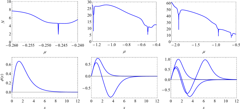
Figure 1: Norm, as defined by Eq. (5), in terms of the trapped soliton frequency (upper row) and the corresponding profiles of the possible bound states of each case (lower row). The values of $\mu$ and $N$ of the sharp dips are: (a) $\mu=-0.245889$, $N=1.8149$ for $j=1$ with bound state profile in (d), (b) $\mu=\{-0.51431,-1.24285\},\,N=\{5.2209,7.96884\}$ for $j=3$ with bound state profiles in (e), and (c) $\mu=\{-0.618207,-0.937341,-1.91964\}$, $N=\{6.0509,8.6734,18.6971\}$ for $j=5$ with bound state profiles in (f). Parameters used: $g_{1}=1/2$, $g_{2}=1$, $\delta=1$, $V_{0}=2$.

Our objective is then to find the possible number of bound states for a fixed norm which we set to be $N=4$. The value of $\delta$ is now varied and the tuning procedure of $\mu$ is repeated for finding all the possible localized solutions of a certain $j$ such that they all have the same norm. The filled circles shown in Fig. 2 represent the coordinates of the localized solutions that all have the norm $N=4$ in terms of the soliton frequency $\mu$ and the parameter $j$. The lines are guides to the eye connecting the localized solutions that share the same number of nodes. The figure suggests that for a specific $j$, the number of possible bound states equals $(j+1)/2$ for odd $j$ and equals $j/2$ for even $j$.

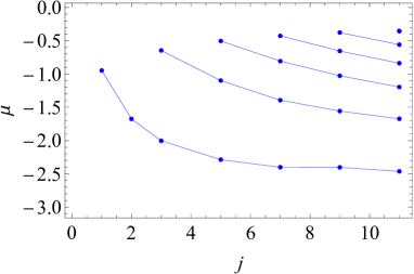
Figure 2: Soliton frequency versus the parameter $j$ for localized solutions that have the norm $N=4$. The lines are guides to the eye. Lines starting from bottom correspond to the 1-, 3-, 5-, 7-, and 9-node trapped modes, respectively. The single isolated filled circle corresponds to the 11-node trapped mode. Parameters used: $g_{1}=1/2$, $g_{2}=1$, $V_{0}=2$.

Our numerical investigation of other potential wells has shown that the main features of their spectra are common. This motivates the investigation of integrable case of SQ potential well in the next section.

III Bound states spectrum of square potential well

By inspection, we found that, in general, bound states spectra exist for a wide range of potential wells and share common main features. This observation will be exploited to understand the main features of the spectrum of the PT potential well. To that end, we consider in this section the finite SQ potential well which is an analytically-solvable model.

III.1 Analytic profile of bound states

The finite SQ potential is defined as follows

$$0,\,\,\,\,\,\,\quad\qquad|x|>1/\alpha,{\qquad\rm(\textit{outside})}$$ (6a)

$$-V_{0},\,\,\qquad|x|<1/\alpha,{\qquad\rm(\textit{inside})}$$ (6b)

where $V_{0}>0$ is the the depth of the potential well and $\alpha=\sqrt{V_{0}}/j$ is its inverse half width, and $j$ is an arbitrary nonezero positive integer. For both regions, inside and outside the potential well, the NLSE is integrable. The solutions we are seeking are oscillatory inside the potential well and decaying outside. The exact solution of the NLSE that describes both cases is the cn Jacobi elliptic function. Inside the potential well, the solution of the NLSE, (4), is denoted by $\phi_{in}(x)$ and outside of the potential well it is $\phi_{out}(x)$. Each one of these solutions contains 4 unknown parameters, as described below. The initial and boundary conditions will be sufficient to determine all unknown parameters. We solve Eq. (4) for each region separately, as follows:

Inside the potential well: In this region, where $V(x)=-V_{0}$, the solution takes the form

$$\phi_{in}(x)=c_{1}\,{\rm cn}[b_{1}(x+{x_{0}}_{1}),m_{1}],$$ (7)

where $c_{1}$, $b_{1}$, ${x_{0}}_{1}$, and $m_{1}$ are real constants to be determined. Direct substitution in Eq. (4), results in the following two equations

$$m_{1}=-\frac{\mu-b_{1}^{2}g_{1}+V_{0}}{2b_{1}^{2}g_{1}},$$ (8)

$$c_{1}=p_{1}\sqrt{\frac{-\mu+b_{1}^{2}g_{1}-V_{0}}{g_{2}}}.$$ (9)

Here, $p_{1}=\pm 1$ and we have used the identities: ${\rm dn}(x,m)=\sqrt{1-m\,{\rm sn}^{2}(x,m)}\,$ and $\,{\rm sn}(x,m)=\sqrt{1-{\rm cn}^{2}(x,m)}$. Without loss of generality, we choose here and below to express all 7 unknown parameters in terms of $b_{1}$.

Outside of the potential well: In this region, $V(x)=0$, and similarly, the solution takes the form

$$\phi_{out}(x)=c_{2}\,{\rm cn}[b_{2}(x+{x_{0}}_{2}),m_{2}],$$ (10)

with new four parameters $c_{2}$, $b_{2}$, ${x_{0}}_{2}$, and $m_{2}$, to be determined. Substituting in Eq. (4), we obtain

$$m_{2}=\frac{1}{2}-\frac{\mu}{2b_{2}^{2}g_{1}},$$ (11)

$$c_{2}=p_{2}\sqrt{\frac{-\mu+b_{2}^{2}g_{1}}{g_{2}}},$$ (12)

where, $p_{2}=\pm 1$ is independent from the sign of $p_{1}$.

Initial condition: Here, we apply the initial condition that will determine the unknown parameter ${x_{0}}_{1}$. The initial condition associated with a wave solution depends on the parity of the solution. Since we are restricted to the symmetric odd parity solutions, the two initial conditions will be: $\phi_{in}(0)=0$ and $d/dx\phi_{in}(x)|_{x=0}$ is arbitrary. Accordingly, we have

$$c_{1}{\rm cn}[b_{1}\,{x_{0}}_{1},m_{1}]=0.$$ (13)

Solving for ${x_{0}}_{1}$, we get

$${x_{0}}_{1}=\frac{{\rm K}(m_{1})}{b_{1}},$$ (14)

where ${{\rm K}(m_{1})}$ is the complete elliptic integral of the first kind.

Boundary conditions: Here, we apply the boundary conditions that will determine two more unknown parameters. The continuity of the solution and its first derivative at $x=1/\alpha$, are expressed as

$$\phi_{in}(1/\alpha)=\phi_{out}(1/\alpha),$$ (15)

$$\frac{d}{dx}\phi_{in}(x)\Big{|}_{1/\alpha}=\frac{d}{dx}\phi_{out}(x)\Big{|}_{1/\alpha}.$$ (16)

Solving (15) for $x_{02}$ and (16) for $b_{2}$, we, respectively, get

$$x_{02}=-\frac{1}{\alpha}+\frac{p_{3}}{b_{2}}\,{\rm cn}^{-1}\left(\frac{c_{2}}{\phi_{0}},m_{2}\right),$$ (17)

$$b_{2}=\frac{p_{2}}{\sqrt{g_{1}}}\left[\mu^{2}+2\mu\phi_{0}^{2}g_{2}+g_{2}(2\phi_{1}^{2}g_{1}+\phi_{0}^{4}g_{2})\right]^{1/4},$$ (18)

where we have introduced

$$\phi_{0}=c_{1}\,{\rm cn}\left[b_{1}\left(\frac{1}{\alpha}+x_{01}\right),m_{1}\right],$$ (19)

$$\phi_{1}=-b_{1}c_{1}\,{\rm dn}\left[b_{1}\left(\frac{1}{\alpha}+x_{01}\right),m_{1}\right]{\rm sn}\left[b_{1}\left(\frac{1}{\alpha}+x_{01}\right),m_{1}\right],$$ (20)

and $p_{3}=\pm 1$ is independent from the signs of $p_{1}$ and $p_{2}$.

Up to this point, all unknown parameters are determined in terms of a single arbitrary parameter, namely $b_{1}$. It is just our choice to leave out this parameter as the arbitrary one; it could have been any other parameter instead. In the following, we impose the restriction that the solutions have to decay to zero outside the potential, which is justified by seeking localized states. This condition will, essentially, determine the last unknown parameter and the system of 8 unknowns will be fully determined.

Localization condition: Here, an additional condition is introduced for the solution to decay to a zero background. This can be achieved by setting $m_{2}=1$, where the outer solution reduces to $c_{2}\,{\rm cn}[b_{2}(x+x_{02}),1]=c_{2}\,{\rm sech}[b_{2}(x+x_{02})]$, which satisfies (4) for

$$c_{2}=p_{2}\,\sqrt{\frac{-2\mu}{g_{2}}},$$ (21)

$$b_{2}=p_{2}\,\sqrt{\frac{-\mu}{g_{1}}}.$$ (22)

Substituting for $b_{2}$ from (18) in (11) with $m_{2}=1$, we get the following transcendental equation for $\mu$

$$q(\mu)=\mu+\sqrt{b_{1}^{4}g_{1}^{2}-V_{0}(V_{0}+2\mu)+2V_{0}(-b_{1}^{2}g_{1}+V_{0}+\mu)\,{\rm cn}^{2}\left[b_{1}\left(\frac{1}{\alpha}+x_{01}\right),m_{1}\right]}=0.$$ (23)

The roots of this equation give the eigenfrequencies of localized modes. It is also noticed that Eqs. (21) and (22) restrict $\mu$ to be negative. Furthermore, we will show next that real-valued solution profiles are obtained only for values of $\mu$ between two limits, which we denote by $\mu_{1}$ and $\mu_{2}$. The limit $\mu_{1}$ is defined by the maximum value of $\mu$ for which the quantity under the square root in Eq. (9) is positive and thus $c_{1}$ is real. Setting $c_{1}=0$ in (9), gives

$$\mu_{1}=b_{1}^{2}g_{1}-V_{0}.$$ (24)

This equation defines a threshold value on $b_{1}$, namely ${b_{1}}_{th}=\sqrt{V_{0}/g_{1}}$, for which $\mu_{1}=0$. For $\mu\leq\mu_{2}$, the quantity $x_{01}$ given by (14) diverges or becomes complex. Therefore, the value of $\mu_{2}$ is easily obtained from Eq. (8) with $m_{1}=1$, which gives

$$\mu_{2}=-b_{1}^{2}g_{1}-V_{0}.$$ (25)

To conclude, only roots of $q(\mu)$ located within the interval $(\mu_{2},\mu_{1})$ lead to solutions with real-valued profiles. In case $b_{1}\geq{b_{1}}_{th}$, Eq. (24) shows that $\mu_{1}>0$. Since acceptable roots require $\mu<0$, then the interval becomes $(\mu_{2},0)$.

Normalization: The total normalization $N$ is the sum of the inner and outer norms, $N_{in}$ and $N_{out}$, respectively. Analytically, it is given by

$$N(\mu)=N_{in}+N_{out} = 2\int_{0}^{1/\alpha}|\phi_{in}(x)|^{2}dx+2\int_{1/\alpha}^{\infty}|\phi_{out}(x)|^{2}dx,$$ (26)

$$= \frac{2c_{1}^{2}}{b_{1}m_{1}\alpha}\left(b_{1}(m_{1}-1)-\alpha\,{\rm E}(m_{1})+\alpha\,{\rm E}\left\{{\rm am}\left[\frac{b_{1}}{\alpha}+{\rm K}(m_{1}),m_{1}\right],m_{1}\right\}\right)$$

$$+\frac{2c_{2}^{2}}{b_{2}}\left\{1-{\rm tanh}\left[b_{2}\left(\frac{1}{\alpha}+x_{02}\right)\right]\right\}.$$

The second and third lines in the last equation correspond to $N_{in}$ and $N_{out}$, respectively, ${\rm E}(\cdot)$ is the elliptic integral of the second kind and ${\rm am}(\cdot)$ is the amplitude of the Jacobi elliptic function. The prefactor $2$ in front of the integrals accounts for the complete domain $[-\infty,\infty]$.

III.2 Constructing the spectrum

Since the norm is a conserved quantity, we aim at constructing the spectrum of bound states for a fixed norm. Taking into account Eqs. (8, 9, 14, 19, 20, 21, 22), the transcendental Eqs. (23) and (26) will be given in terms of only $b_{1}$ and $\mu$. In order to obtain a spectrum with fixed norm, we need to set a value of $N(\mu)$ in (26) and then solve the system (23) and (26) for $b_{1}$ and $\mu$. The resulting roots of (23) will give the eigenfrequencies of the bound states. However, this procedure turns out to be not practical since it requires solving two coupled transcendental equations simultaneously. Alternatively, we follow the following approach. We consider a range of $b_{1}$ values, compute the roots of $q(\mu)$ for each value of $b_{1}$, calculate the associated norm for each root, and then extract from this collection of data the roots which have the same norm.

In Fig. 3, we clarify the procedure just described for an example of SQ potential well characterized by $V_{0}=2$ and $j=3$. The left column of the figure corresponds to the case $b_{1}<{b_{1}}_{th}$. The shaded area is used to identify the range of acceptable roots limited by $\mu_{1}>\mu>\mu_{2}$. The limits $\mu_{1}$ and $\mu_{2}$ are indicated by two vertical dashed (red) lines. One eigenfrequency is found at $\mu=-1.3695$ corresponding to a single-node trapped mode. The case of $b_{1}={b_{1}}_{th}$ is shown in the middle column of subfigures. The roots range of this case is $0>\mu>\mu_{2}$, where $\mu_{1}=0$. Similarly, only one root at $\mu=-3.6025$ is found. The profile of the corresponding single-node trapped mode is different than the previous one. The last case, shown in the right column of subfigures, is for $b_{1}>{b_{1}}_{th}$. Here, three roots appear at $\mu=\{-0.9075,-2.5135,-4.6585\}$ and labeled by $\{a,b,c\}$, respectively. As we mentioned above, the acceptable roots of this case are in the range $0>\mu>\mu_{2}$. Interestingly, both $a$ and $b$ wave frequencies form two distinguishable triple-node trapped modes. An important difference between them should be noted. The mode corresponding to root $a$ has constant maximum amplitude in the oscillatory part. For the mode corresponding to root $b$, the peaks at both edges are larger than those in between. We denote the two cases by symmetric and asymmetric profiles, respectively. It should be also noted that the three single-node trapped modes in the three cases are all different from each other.

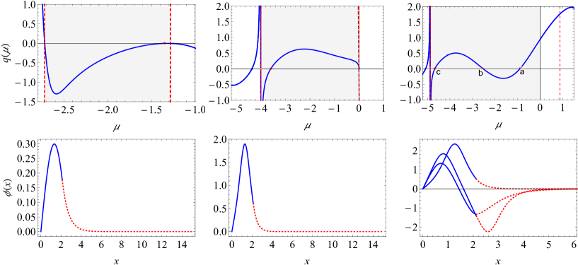
Figure 3: Eiegen frequencies and eigen modes for three cases of $b_{1}$. The upper row shows the real roots of Eq. (23) and the lower row presents the corresponding wave profile, (a) and (d) for $b_{1}<{b_{1}}_{th}$ $(=0.6\,{b_{1}}_{th})$, with a single root at $\mu=-1.3695$, (b) and (e) for $b_{1}={b_{1}}_{th}$ with a single root at $\mu=-3.6025$, and (c) and (f) for $b_{1}>{b_{1}}_{th}$ $(=1.2\,{b_{1}}_{th})$, with three roots at $\mu=\{-0.9075,-2.5135,-4.6585\}$. Filled (red) circles indicate roots, dashed (red) vertical lines indicate the positions of $\mu_{1}$ (right) and $\mu_{2}$ (left), and the area of included $\mu$ is shaded. Parameters used: $g_{1}=1/2$, $g_{2}=1$, $V_{0}=2$, $j=3$.

The desired smooth and continuous matching between the inner and outer solutions is attained with $p_{1}=p_{2}=1$. The required sign of $p_{3}$ is obtained by matching the slopes of the inner and outer solutions at the edge of the potential. This can be done by equating $\phi_{1}$ from Eq. (20) to a similar expression but with subscripts $1$ being replaced by $2$.

Constructing the spectrum, starts, as we described above, with finding the roots of (23) for a range of $b_{1}$ values. The result is shown in Fig. 4. The figure shows three curves which correspond, starting from the bottom, to single-node trapped modes and two triple-node trapped modes. No roots exist for $b_{1}<1.1632$, which is indicated by the vertical dashed (pink) line. A single value of $\mu$ is obtained for a wide range of $b_{1}$, varying from 1.1632 to 2.25169, which is indicated by the region in between the vertical dashed (pink) and solid (green) lines. Three values of $\mu$ are found for $b_{1}>2.25169$. As an example, we draw a vertical dotted (red) line at $b_{1}=2.4$ that crosses the three roots shown in Fig. 3(c). Their corresponding profiles are those shown in Fig. 3(f).

Calculating the norm of modes corresponding to all points in Fig. 4, the relation between $N(\mu)$ and $\mu$ of the three curves can be extracted and is plotted in Fig. 5(a). Interestingly, only single-node trapped modes are observed to occur with the norm range $N<6.3916$. Larger norm is needed for the formation of higher nodes trapped modes. Two distinguishable triple-node trapped modes are formed for $N>6.3916$. The dotted (red) line crosses three roots corresponding, starting from the lowest curve, to a single-, asymmetric triple-, and symmetric triple-node trapped modes, all with the same norm, $N\approx 12$. Figure 5(b) shows a zoom of the point at which the two branches of triple-node trapped modes appear. The upper branch connected by the dashed (black) line corresponds to symmetric triple-node trapped modes while the lower branch connected by the solid (red) line corresponds to the asymmetric triple-node trapped modes.

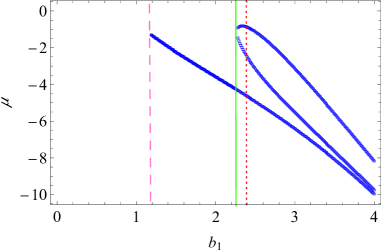
Figure 4: Mode frequency, $\mu$, in terms of $b_{1}$. The curves from the bottom of the figure correspond to single-, symmetric triple-, and asymmetric triple-node trapped modes, respectively. The dashed (pink) line defines the range $b_{1}\leq 1.1632$ for which no eigenmodes exist. The solid (green) line at $b_{1}=2.25169$ indicates the starting value of triple-node trapped mode formation with the presences of single-node trapped mode. The dotted (red) line at $b_{1}=2.4$ is an example capturing three modes from the bottom of the figure at $\mu=\{-0.9075,-2.5135,-4.6585\}$. Parameters used: $g_{1}=1/2$, $g_{2}=1$, $V_{0}=2$, $j=3$, $0.5\,{b_{1}}_{th}\leq b_{1}\leq 2\,{b_{1}}_{th}$.

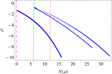
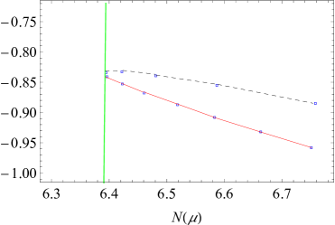
Figure 5: Possible wave frequencies $\mu$ in terms of normalization $N(\mu)$. The curves from the bottom of the figure (a) correspond to the same curves in Fig. 4. The dashed (pink) line detects the value of $N=0.06972$ at which no $\mu$ is detected before. The solid (green) line at $N=6.3916$ indicates the minimum value that supports the formation of triple-node mode with the presences of single-node mode. The (red) dotted line at $N=12$ is an example supporting three modes at $\mu=\{-5.7785,-4.6035,-2.2035\}$ from the bottom of the figure, respectively. A zoom-in portion of the plot in (a) is shown in (b) where dashed (black) curve corresponds to asymmetric triple-node modes and solid red curve corresponds to symmetric triple-node modes. Parameters used are the same of those in Fig. 4.

For the sake of comparison, we show in Fig. 6(a), the single-node trapped mode profiles of the PT and SQ potential wells using the same set of parameters. The profiles of the triple-node trapped modes are shown as well in Fig. 6(b). While there are three trapped modes formed in the SQ potential spectrum, only two modes are formed in the PT potential spectrum. Inspection shows that the spectrum of the SQ potential well is always composed by a finite number of bound states determined by the norm $N$ and the value of $j$. As $N$ increases, the number of bound states with the same $j$ increases. However, in the case of the PT potential, only the parameter $j$ determines the number of the bound states in the spectrum regardless of the norm. Increasing the norm in the case of PT potential will not change the number of possible bound states in the spectrum. Table 1 summarizes the norm, $N$, energy, $E_{T}$, number of nodes, $n$, critical speed for quantum reflection, $v_{c}$ (defined in Sec. III.3), of bound states for the two spectra. In Fig. 7(a), we show a schematic diagram of the spectrum for the PT potential, that is constructed by a single-node and triple-node trapped modes with trapped mode energies $E_{1}$ and $E_{3}$. Figure 7(b), shows as well the schematic diagram of the spectrum for the SQ potential that consists of a single-, symmetric-, and asymmetric-node trapped modes with trapped mode energies $E_{1},E_{3}^{1},$ and $E_{3}^{2}$, respectively.

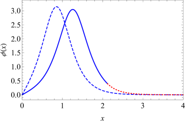
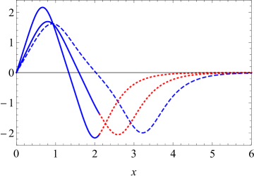
Figure 6: Profiles of the single-node (a) and triple-node (b) trapped modes of the SQ and PT potential wells. Dashed curves correspond to PT potential well and solid (blue) and dotted (red) curves correspond to the SQ potential well. Parameters used: $g_{1}=1/2$, $g_{2}=1$, $V_{0}=2$, $j=3$.

$\begin{array}[]{c|c|c|c|c}\hline\cr\lx@intercol\hfil\rm\quad PT\,\,potential\hfil\lx@intercol\\ \hline\cr\mu&n&N&E_{T}&v_{c}\\ \hline\cr$-6.4660$&1&12.0465&$-37.3273$&$2.42816$\\ \hline\cr$-2.22655$&3^{*}&12.0270&$-12.3972$&3.16110\\ \hline\cr\lx@intercol\hfil\rm\quad SQ\,\,potential\hfil\lx@intercol\\ \hline\cr$-6.6085$&1&12.0469&$-42.0890$&2.25976\\ \hline\cr$-2.5575$&3&12.0362&$-11.0984$&3.19818\\ \hline\cr$-2.1155$&3^{*}&12.0271&$-9.62501$&3.23320\\ \hline\cr\end{array}$

Table 1: Norm, $N$, energy, $E_{T}$, number of nodes, $n$, critical speed, $v_{c}$, of bound states for the SQ and PT potential wells with parameters corresponding to Fig. 6. The 3-node trapped modes distinguished by $*$ correspond to the asymmetric modes.

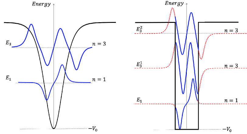
Figure 7: Schematic diagrams of the spectra of bound states for: (a) PT potential well, (6), with $E_{1}$ and $E_{3}$ corresponding to the trapped energies of the single- and triple-node trapped modes, respectively, and (b) SQ potential well, (2), with $E_{1},E_{3}^{1},$ and $E_{3}^{2}$ corresponding to the trapped energies of the single-, symmetric triple-, and asymmetric triple-nodes trapped modes the PT potential well. Parameters used are those of Fig. 6.

We show in Fig. 8 other cases including the reflectionless potential with $j=1$, and for a case with $j=2$. A significant difference between the two potential wells should be noted. While the reflectionless PT potential does not support other than single-node trapped modes usa1 , the SQ potential, supports in addition to the single-node trapped mode, multi-node trapped modes. In fact, with the SQ potential well characterized by $\alpha=\sqrt{V_{0}}$, multi-node trapped modes do form. The figure shows up to triple-node trapped modes. With the same maximum value in the $b_{1}$ range for the case of $\alpha=\sqrt{V_{0}}/2$, the triple-node trapped modes are observed to occur earlier than what was in the former situation. Moreover, two branches of quintuple-node trapped modes start to form.

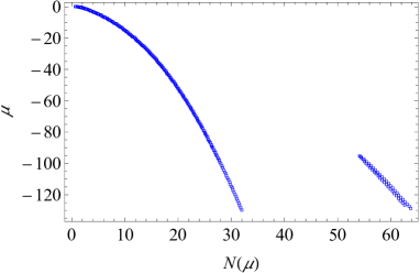
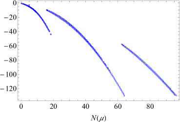
Figure 8: Possible eigenfrequencies in terms of normalization $N(\mu)$ for (a) $j=1$ with $0.9\,{b_{1}}_{th}\leq b_{1}\leq 8\,{b_{1}}_{th}$ and (b) $j=2$ with $0.7\,{b_{1}}_{th}\leq b_{1}\leq 8\,{b_{1}}_{th}$. The left curve in (a) corresponds to single-node trapped modes while the right curve is composed of two curves corresponding to triple-node trapped modes. In (b), the left curve corresponds to single-node modes, the middle curve is composed of two curves both correspond to two triple-node trapped modes, and the right curve is also composed of two curves both correspond to quintuple-node trapped modes. Parameters used: $g_{1}=1/2$, $g_{2}=1$, $V_{0}=2$.

III.3 Critical speed for quantum reflection

The derivation of the critical speed for quantum reflection is based on the conservation law of energy. The critical speed can be obtained by equating the initial energy of the incoming soliton to that of the trapped mode at the centre of the potential well. This leads to an analytic formula for the critical speed, as was shown for the PT potential well usa1 . Considering the same scenario for the SQ potential well, the critical speed reads

$$v_{c}=\sqrt{\frac{1}{12}g_{2}^{2}N^{2}+\frac{2}{N}E_{T}},$$ (27)

where $N$ is given by $(\ref{norm})$ and $E_{T}$ is the energy of the trapped mode given by

$$E_{T}=E_{in}+E_{out} = N_{in}\,\mu+2\times\frac{g_{2}}{2}\int_{0}^{1/\alpha}|\phi_{in}(x)|^{4}dx+N_{out}\,\mu+2\times\frac{g_{2}}{2}\int_{1/\alpha}^{\infty}|\phi_{out}(x)|^{4}dx$$ (28)

$$= N\,\mu+\int_{0}^{1/\alpha}|\phi_{in}(x)|^{4}dx+\int_{1/\alpha}^{\infty}|\phi_{out}(x)|^{4}dx.$$

Figure 9 shows the relation between the trapped mode energy $E_{T}$ and the norm $N$ for the same case of Fig. 5. Using the same parameters of those in Fig. 9, in Fig. 10, we plot the dependence of the critical speed for quantum reflection on the trapped mode energy. Three curves are shown in the left subfigure that correspond to the single- and two triple-node trapped modes. Although the upper two curves for the symmetric and asymmetric triple-node trapped modes seem to have the same $v_{c}$, there is a notable difference which is verified by taking a zoom in part of the curves, as shown in the right subfigure. The vertical dashed (pink) line indicates the minimum norm $N\approx 6$ that is required for the quantum reflection to occur with a triple-node trapped mode. Quantum reflection by the single-node trapped mode is observed to start at $N\approx 7.6$, as indicated by the solid (green) line.

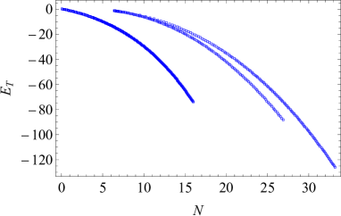
Figure 9: Energy of trapped modes $E_{T}$ in terms of the norm $N$. The curves from the bottom of the figure correspond to the same curves in Fig. 4. Parameters used are the same of those in Fig. 4.

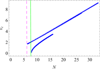
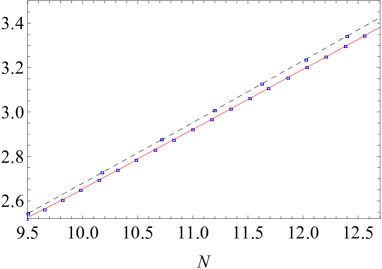
Figure 10: Critical soliton speed, $v_{c}$, in terms of full normalization $2N$ at which the soliton will be trapped by the potential well (6) forming the modes discussed in Fig. 5. The triple-node modes start to be trapped as a result of soliton quantum reflection with $N\approx 6$, while the single-node trapped modes with $N\approx 7.6$. This is indicated by the solid (green) line. A zoom-in portion of the indistinguishable part in plot (a) is shown in (b) where the dashed (black) curve corresponds to asymmetric triple-node trapped modes and solid (red) curve corresponds to symmetric triple-node trapped modes. Parameters used are the same of those in Fig. 4.

IV Resonant soliton scattering

In this section, we consider the scattering of a bright soliton by the PT and SQ potential wells in order to confirm the exitance and the above-described features of the bound states spectrum. In addition, quantum reflection and its critical speed values will be also confirmed. This will be followed by a theoretical proof explaining the specific number of nodes in the excited trapped modes. This will be based on the modulational instability analysis of the excited bound state.

IV.1 Scattering dynamics

Here we describe the scattering setup of a soliton-potential interaction governed by Eq. (1). To account for the theoretical analysis we have made in the previous two sections, we consider here the scattering of the soliton in two setups; in the presence of the PT potential well and in the presence of the SQ potential well, separately. As an incident soliton, in the two setups, we use the exact movable bright soliton solution to the fundamental NLSE, namely, Eq. (1) with $V(x)=0$, given in a normalized form as book

$$\psi(x,t)=N\sqrt{\frac{{g_{2}}}{8{g_{1}}}}\,\text{sech}\left[\frac{{g_{2}}N(x-{x_{0}}-vt)}{4{g_{1}}}\right]e^{\frac{i}{16g_{1}}\left[\left({g_{2}}^{2}N^{2}-4v^{2}\right)t+8v\left(x-{x_{0}}\right)\right]},$$ (29)

where $x_{0}$ and $v$ are the initial position and speed of the soliton centre, and $N$ is its norm given by Eq. (5). The scattering outcome is determined by solving numerically Eq. (1) using the iterative power series method num with $\psi(x,0)$ from Eq. (29) as an initial profile. Scattering dynamics of the soliton described by (29) at $t=0$ with the PT potential $V(x)=-65\,{\rm sech}^{2}(\sqrt{65}\,x/3)$ and norm $N=4$ is presented in Fig. 11(a) where it shows clearly the formation of a triple-node trapped mode at the centre of the potential well. In Fig. 11(b) we plot the corresponding profiles of the trapped mode obtained by direct numerical solution of the (1) and the profile obtained from the scattering simulation at the classical turning point. The two profiles show an agreement on the number and location of the nodes. However, since the trapped mode is not fully occupied due to radiation, as the potential is not reflectionless, the maxima in the profile obtained by the scattering experiment are less than those of the direct numerical solution. The lower row of the same figure represents the outcome of the scattering process but with a SQ potential well characterized by $V_{0}=2$ and $j=3$. While the numerical scattering experiment shows a similar result to that in the PT potential case, the formed triple-node mode here is accompanied with considerable reflected and transmitted portions, as shown in Fig. 11(c). Similar to the PT case, the profiles in Fig. 11(d), show agreement between the scattering results and the direct numerical solution on the number and location of nodes. However, the discrepancy between the amplitudes of the profiles is larger due to considerable reflection and transmission.

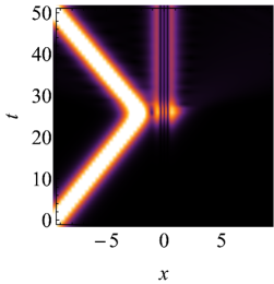
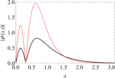
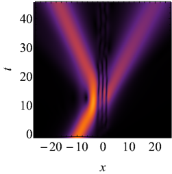
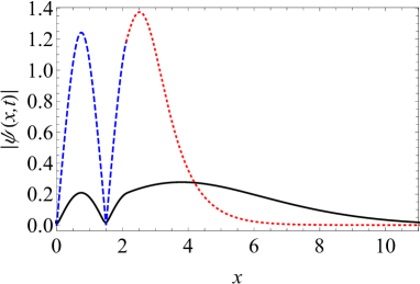
Figure 11: Formation of a triple-node trapped node as a result of the soliton described by (29) at $t=0$ scattered by (a) the PT potential $V(x)=-65\,{\rm sech}^{2}(\sqrt{65}x/3)$ and $N=4$ and by (c) the SQ potential (6) with $V_{0}=2$ and $N=1$. (b) Profile of the maximally occupied trapped mode where the dotted (red) curve is the result of the numerical solution of Eq. (4) and the solid (black) curve is the maximally occupied trapped mode obtained by the scattering shown in subfigure (a). (d) Profile of the maximally occupied trapped mode where the dashed blue and dotted red curves are the result of the exact solution of Eq. (4) with $N=7$ and the solid (black) curve is the maximally occupied trapped mode obtained by the scattering shown in subfigure (c). Parameters used: $g_{1}=1/2$, $g_{2}=1$, $j=3$.

We have found that, whether the potential is the PT or the SQ potential well, the scattering process always excites only one bound state with $j$ number of nodes. A physical explanation of this phenomenon will be provided by modulational instability analysis in the next subsection.

IV.2 Modulational instability analysis

As discussed above, for each value of $j$, there is a finite number of eigenmodes. However, only the mode with maximum number of nodes, that is equal to $j$, is excited by the scattering process. The aim of this section is to explain this behaviour. To that end, we employ a MI analysis. Modulational instability is typically caused by perturbations on a static solution growing up exponentially with time to either blow up or sometimes form another solution.

We will start by performing the typical MI analysis of a finite background for the homogeneous NLSE. This will give the frequency of the most unstable mode. Then, we consider the most unstable mode within the potential well and apply the boundary conditions to obtain the relation between the number of nodes and the potential width.

The so-called constant wave (CW) solution of Eq. (1) inside a SQ potential well with depth $V_{0}$ is given by

$$\psi_{0}(x,t)=Ae^{i(A^{2}\,g_{2}+V_{0})t},$$ (30)

where $A$ is an arbitrary real constant. Introducing a small perturbation $\psi_{1}(x,t)$ to the CW solution such that $|\psi_{1}(x,t)|<<|\psi_{0}(x,t)|$, we have

$$\psi(x,t)=[A+\psi_{1}(x,t)]e^{i(A^{2}\,g_{2}+V_{0})t}.$$ (31)

Substituting in Eq. (1) and linearizing in $\psi_{1}(x,t)$, we get

$$i\frac{\partial}{\partial t}\psi_{1}(x,t)+g_{1}\frac{\partial^{2}}{\partial x^{2}}\psi_{1}(x,t)+A^{2}\,g_{2}[\psi_{1}(x,t)+\psi_{1}^{*}(x,t)]=0.$$ (32)

We assume the perturbation form

$$\psi_{1}(x,t)=Ue^{i(\omega\,t-k\,x)}+Ve^{-i(\omega\,t-k\,x)},$$ (33)

where $k$ and $\omega$ are the wavenumber and frequency of the perturbation, respectively, and $U$ and $V$ are arbitrary real constants. Substituting in the linearized equation (32), results in

$$(A^{2}g_{2})U+(A^{2}g_{2}-g_{1}k^{2}+\omega)V=0,$$ (34)

$$(A^{2}g_{2}-g_{1}k^{2}-\omega)U+(A^{2}g_{2})V=0.$$ (35)

The condition for nontrivial solution yields the dispersion relation

$$\omega=\sqrt{g_{1}k^{2}(-2\,A^{2}\,g_{2}+g_{1}\,k^{2})}.$$ (36)

The imaginary part of $\omega$ has a maximum at

$$k=\pm A\sqrt{\frac{g_{2}}{g_{1}}}.$$ (37)

This value corresponds to the most unstable mode. Substituting back in the dispersion relation (36), the maximum real part of the frequency is obtained to be $\omega=A^{2}g_{2}$. This is the frequency of the dominant mode that will determine the fate of the instability.

Requiring the most unstable CW solution to satisfy the boundary conditions at the edges of the potential well, defines a specific wavenumber, which we denote as $k_{2}$, that depends on the width of the potential. The CW solution then reads

$$\psi_{0}(x,t)=Ae^{i(\omega\,t-k_{2}\,x)}.$$ (38)

For this CW to be a solution to the NLSE, (1), the wave number must satisfy

$$k_{2}=\pm\sqrt{\frac{V_{0}}{g_{1}}}.$$ (39)

Expressing $k_{2}$ in terms of the wavelength of the trapped mode, $\lambda$, as $k_{2}=2\pi/\lambda$, Eq. (39) gives $\lambda=(2\pi\sqrt{g_{1}})/\sqrt{V_{0}}$. We define the ratio between the width of the potential well $W=2/\alpha=2j/\sqrt{V_{0}}$ and $\lambda$, as $l=W/\lambda$, which corresponds to the number of waves inside the potential well. Since each wavelength contributes with 2 nodes, the number of nodes predicted by MI is given by $n_{MI}=2l$. We finally obtain the number of nodes

$$n_{MI}=\frac{2}{\pi\sqrt{g_{1}}}\,j.$$ (40)

Since the prefactor ${2}/{\pi\sqrt{g_{1}}}\approx 0.9$, the last formula provides an explaination for the number of nodes in the trapped modes being equal to $j$. Interestingly, the number of nodes does not depend on $V_{0}$.

As an illustrative example, the formation of a multi-node trapped mode for the SQ potential well characterized by $V_{0}=50$ and $j=7$ and $N=1$ is shown in Fig. 12. The figure shows clearly the formation of a trapped mode with 7 nodes. The profile of the maximally occupied trapped mode obtained by the scattering is also shown in the left subfigure together with its real and imaginary parts.

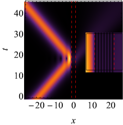
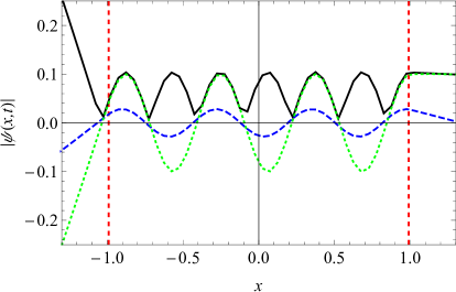
Figure 12: (a) Formation of trapped node with 7 nodes as a result of the soliton described by (29) at $t=0$ scattered by the SQ potential well (6). (b) Profile of the maximally occupied trapped mode where the profile and its real and imaginary parts are indicated by solid (black), dashed (blue), and dotted (green) curves, respectively. The dashed red vertical lines indicate the borders of the potential well width. Inset in (a) shows a zoom-in of the scattering near the potential region. Parameters used: $g_{1}=1/2$, $g_{2}=1$, $V_{0}=50$, $j=7$, $N=1$.

V Summary and CONCLUSIONS

We have revealed the structure of bound states spectrum for a modified PT potential well. Bound states were obtained through direct numerical solution of the NLSE, Eq. (1), using the potential well (2). Tuning the central profile slope and the frequency, a localized solution with decaying tail is obtained. The solutions turn out to be characterized by the number of nodes, their norm, and their energy. A more efficient alternative method is to calculate the norm of the numerical solutions for a range of frequencies where localized solutions will be identified with sharp dips in the curve, as shown in Fig. 1.

For a fixed norm, it turns out that a finite number of eigenmodes exit. Each eigenmode is associated with an eigenfrequency. Interestingly, the positive nonzero integer $j$, which is used to define the inverse width of the potential, $\alpha=\sqrt{V_{0}}/j$, determines the numbers of possible eigenmodes and their nodes, as follows. For a given $j$, eigenmodes exist with an odd integer number of nodes, $n$, such that $1\leq n\leq j$. The total number of eigenmodes is then $(j+1)/2$ or $j/2$ for $j$ being odd or even integer, respectively. This gives the following general structure of the spectrum: it is a finite number of localized eigenmodes each characterized by its unique number of nodes and eigenfrequency. Obviously, for $j=1$, which corresponds to the reflectionless potential case, there is only one eigenmode which has a single node. This is the well-known trapped mode responsible for quantum reflection well1 ; impu4 ; usa6 . It should be noted that the general structure of the spectrum will not be changed by changing the norm, $N$; it will affect only the amplitude of eigenmodes profiles.

Motivated by the finding that the general structure of the spectrum of bound states is a common feature for a wide class of potential wells, we considered the same problem for the SQ potential well. In this case, the problem is analytically solvable in terms of the Jacobi elliptic functions. The spectrum turns out to be, indeed, similar to that of the PT potential well, but with the difference that the number of eigenmodes increases with increasing $N$. In addition, a degeneracy was found where more than one eigenmode having the same number of nodes, as for instance the two 3-nodes eigenmodes in Fig. 7, which we denoted as symmetric and asymmetric modes.

Bound states have an important effect on quantum reflection and the sharp transition in transport coefficients of soliton scattering. For both potentials, the critical speed for quantum reflection was calculated using the eigenenergies of the bound states, as summarized in Table 1.

Exciting bound states can be performed by resonant soliton scattering with the potential at the critical speed for quantum reflection. Indeed, the numerical experiments show the formation of trapped modes at the potential with the correct predicted number of nodes, as shown in Fig. 12. There is no agreement though between the predicted amplitude and the one obtained from scattering simulation. This is due to the radiation losses and the fact that in the SQ potential well, there is a considerable amount of reflected and transmitted intensities, and thus the trapped mode is not fully populated.

We have presented a theoretical explanation, based on modulational instability analysis, for the relation between the predicted number of nodes, $n_{MI}$, and the integer $j$, as was described above. This resulted in formula (40) which gives accurately the predicted number of nodes in terms of $j$.

Numerical simulations of soliton scattering by the potential wells, for a specific norm $N$ and number $j$, can only excite the mode with the maximum number of nodes, namely $j$. Therefore, resonant scattering by the trapped modes with lower number of nodes, $n<j$, may not be possible to excite these modes. As an alternative procedure, we suggest that, exciting such trapped modes may be achieved through the phase imprinting method, where the phase extracted from the corresponding analytical solution, is imprinted initially on a stationary soliton located at the potential well. This is left to be investigated in a future work.

References

- (1) F. Baronio, C. De Angelis, P. Pioger, V. Couderc, and A. Barthélémy, Opt. Lett. 29, 986 (2004).
- (2) H. Friedrich and J. Trost, Phys. Rep. 397, 359 (2004).
- (3) R. Cote, H. Friedrich, and J. Trost, Phys. Rev. A 56, 1781 (1997).
- (4) M. Lizunova, O. Gamayun, arXiv:2010.03385 (nlin), (2010).
- (5) Y. Nogami and F.M.Toyama, Phys. Lett. A 184, 245 (1994).
- (6) H. Sakaguchi and M. Tamura, J. Phys. Soc. Jpn. 74, 292 (2005).
- (7) C. Weiss and Y. Castin, Phys. Rev. Lett. 102, 010403 (2009).
- (8) O. V. Marchukov, B. A. Malomed, V. A. Yurovsky, M. Olshanii, V. Dunjko, and R. G. Hulet, Phys. Rev. A 99, 063623 (2019).
- (9) V. Dunjko, M. Olshanii, arXiv:1501.00075v4 (2020).
- (10) C. Lee and J. Brand, Europhys. Lett. 73, 321 (2006).
- (11) T. Ernst and J. Brand, Phys. Rev. A. 81, 033614 (2010).
- (12) A. E. Miroshnichenko, S. Flach, and B. Malomed, Chaos 13, 874 (2003).
- (13) K. T. Stoychev, M. T. Primatarowa, and R. S. Kamburova Phys. Rev. E 70, 066622 (2004).
- (14) K. Forinash, M. Peyrard, and B. Malomed, Phys. Rev. E 49, 3400 (1994).
- (15) X. Cao and B. Malomed, Phys. Lett. A 206, 177 (1995).
- (16) D. J. Frantzeskakis, G. Theocharis, F. K. Diakonos, P. Schmelcher, and Y. S. Kivshar, Phys. Rev. A 66, 053608 (2002).
- (17) R. H. Goodman, P. J. Holmes, and M. I. Weinstein, Physica D 192, 215 (2004).
- (18) V. A. Brazhnyi and M. Salerno, Phys. Rev. A 83, 053616 (2011).
- (19) M. O. D. Alotaibi and L. D. Carr, J. Phys. B, Mol. Opt. Phys. 52, 165301 (2019).
- (20) T. Ernst and J. Brand, Phys. Rev. A. 81, 033614 (2010).
- (21) M. Asad-uz-zaman and U. Al Khawaja, Europhysics Letters), 101, 50008 (2013).
- (22) U. Al Khawaja and Andery A. Sukhorukov, Optics Letters, 40, 2719 (2015).
- (23) U. Al Khawaja, S. M. Al-Marzoug, and H. Bahlouli, Physics Letters A 384, 126625 (2020).
- (24) R. H. Goodman, P. J. Holmes, and M. I.Weinstein, Physica D 192, 215 (2004).
- (25) T. Ernst and J. Brand, Phys. Rev. A. 81, 033614 (2010).
- (26) U. Al Khawaja, Phys. Rev. E 103, 062202 (2021).
- (27) T. Uthayakumar, L. Al Sakkaf, and U. Al Khawaja, Phys. Rev. E 104, 034203 (2021).
- (28) L. Al Sakkaf, T. Uthayakumar, and U. Al Khawaja, Quantum reflection of dark solitons scattered by reflectionless potential barrier and position-dependent dispersion, Phys. Rev. E (Nov. 2021), submitted.
- (29) U. Al Khawaja, and L. Al Sakkaf, Handbook of Exact Solutions to the Nonlinear Schrödinger Equations, IOP Publishing Ltd 2020, London. Online ISBN: 978-0-7503-2428-1, Print ISBN: 978-0-7503-2426-7.
- (30) U. Al Khawaja and Q. M. Al-Mdallal, Int. J. Diff. Eq. 2018, 6043936 (2018); L. Al Sakkaf, Q. M. Al-Mdallal, and U. Al Khawaja, Complexity 2018, 8269541 (2018); L. Al Sakkaf and U. Al Khawaja, arXiv:2108.00936