Quantum reflection of dark solitons scattered by reflectionless potential barrier and position-dependent dispersion

Abstract

We investigate theoretically and numerically quantum reflection of dark solitons propagating through an external reflectionless potential barrier or in the presence of a position-dependent dispersion. We confirm that quantum reflection occurs in both cases with sharp transition between complete reflection and complete transmission at a critical initial soliton speed. The critical speed is calculated numerically and analytically in terms of the soliton and potential parameters. Analytical expressions for the critical speed were derived using the exact trapped mode, a time-independent, and a time-dependent variational calculations. It is then shown that resonant scattering occurs at the critical speed, where the energy of the incoming soliton is resonant with that of a trapped mode. Reasonable agreement between analytical and numerical values for the critical speed is obtained as long as a periodic multi-soliton ejection regime is avoided.

I Introduction

One of the fascinating phenomena observed for bright solitons in nonautonomous nonlinear systems is quantum reflection. In such a phenomenon, the soliton that approaches a potential can be reflected even in the absence of a classical turning point well1 ; well2 . It portrays the wave nature of the soliton. Furthermore, such nonclassical interactions are known to exist only for the solitons approaching with lower velocities. Whereas, if the incident soliton velocity is above a certain critical value, a sharp transition from complete reflection to complete transmission takes place. Subsequent investigations have revealed that such a feature resuls from the formation of localised trapped mode soliton at the centre of the potential. It also signifies the indispensable role of the incident soliton energy relative to the trapped mode energy on the appearance of sharp transition of quantum reflection. Further, an accurate estimation of the critical speed required for quantum reflection considering various potential depths as well as investigating stability of the trapped modes against perturbations for single as well as multi-node trapped modes have also been studied usa . Remarkably, investigations from such systems described the possibility of the high-speed soliton ejection, even for the stationary solitons positioned at a distance sufficiently far from the centre of the potential. These higher ejection speeds are accompanied with multi-node trapped modes that hold larger binding energy usa7 . Quantum reflection of solitons is witnessed in diverse external potentials, for instance, barriers bar0 ; bar1 ; bar2 ; bar3 , wells well1 ; well2 ; well3 ; well4 , steps step1 ; step2 , and surfaces surf1 ; surf2 ; surf3 . Such studies allowed for the understanding of the energy exchange mechanism of the soliton during the scattering process with the potential to implement soliton based diodes, all-optical logic gates, switches and filters using appropriate setups usa1 ; usa2 ; usa3 ; usa4 ; usa5 ; usa6 .

In general, quantum reflection of bright solitons through diverse potentials has been extensively analysed. For instance, in optics, solitons are generated through compensating the group-velocity dispersion (GVD) with the Kerr nonlinearity during its evolution through an optical fiber. In view of nonlinear evolution with the negative GVD (anomalous dispersion), the fiber supports the pulse propagation in the form of sech pulse profile and such stable nonlinear pulses are universally acknowledged as a bright soliton Agrawal ; Agrawal2 ; book . Contrarily, for positive GVD (normal dispersion), the soliton manifests itself as a localized dip in the intensity with a uniform continuous-wave background. These dark solitons also possess the shape and velocity preserving propagation as that of its bright counterpart Hasegawa ; Krokel ; Kivshar . Since its recent theoretical prediction in optical fibers by Hasegawa and Tappert Hasegawa and experimental realization by Emplit et al. Emplit , considerable research efforts have been made to understand the dynamics of dark solitons in various situations under diverse nonlinear systems. In addition, they are observed to be generated without the threshold in the input pulse power Gredeskul . Although dark solitons appear in autonomous systems paramountly, their dynamics in nonautonomous systems has particularly attracted a special interest to understand the diverse real physical situations where complex space-time forces appear Kivshar .

Considering quantum reflection in dark solitons, Cheng, et al., demonstrated the quantum reflection in Bose-Einstein condensates, where condensate comprises a dark soliton subjected to the scattering by a potential barrier. This study discussed the influence of diverse factors, namely, barrier height, width, the orientation angle of the dark soliton and initial displacement of the condensate cloud on the quantum reflection phenomenon. The reflection probability is found to be sensitive to the initial orientation and also influences the excitation process during the condensate and barrier interaction Cheng . A potential in the form of box-like traps also accounted for the investigation of dark soliton dynamics in BEC at zero temperature. Here, the sidewalls of the potential are considered to rise either as Gaussian or a power-law. In such a setup, the soliton is found to propagate through the trap without any dissipation. However, dissipation was observed during the reflection from a wall with the emission of sound waves, resulting in a slight increase in the speed of the solitons. For the multiple oscillations and reflections inside the trap, the energy loss and the speed are found to increase significantly Sciacca . Scattering of dark solitons in a two defect potential inferred that dark solitons cannot be trapped through two identical potential barriers. Moreover, interactions of dark solitons in such a setup is found to increase the speed of the soliton while traversing through the first barrier, which always allows overcoming the second one. This predicted the only possibility to achieve the optical diode based on dark soliton scattering through time-dependent potential barriers tsitoura . An optical event horizon where reversible soliton transformation from black soliton and a gray one to vice versa is demonstrated through the interaction of dark soliton with a probe wave. This reversible transformation of soliton is generated under the competition between the internal phase of the dark soliton and the nonlinear phase shift induced by the probe. Such a system allows the potential application for information cloaking Deng .

The scattering of composite dark-bright solitons through a fixed localized delta impurity is also considered by employing a mean-field approach. The study identified that such interaction excited different modes that result in the emergence of dark-bright soliton with a distinct velocity. Also, accounted for the regions of reflection, transmission, and in addition to the inelastic scattering behaviour with complex internal mode excitations Majed . Recently, Hansen et. al, described the propagation properties of matter wave solitons through the localized scattering potentials and identified the regimes over which solitons can behave as a wave or as a particle as a consequence of the interplay between dispersion and the attractive atomic interactions, through mean-field analysis Hansen . Although numerous investigations were reported for dark solitons scattering in BEC, there is no significant study involving quantum reflection of dark solitonic pulses through scattering by potential barriers. In most of the situations, dark solitons are dealt with and treated in presence of the bright soliton background.

In the present study, we consider the scattering dynamics of dark solitons propagated well far from the centre of an external potential or a region of modulated dispersion in order to investigate the existence and characteristics of quantum reflection. The study has three main objectives: i) to confirm the existence of quantum reflection and to identify the type of potentials (well or barrier) needed for it to occur, ii) to investigate the characteristics of the quantum reflection phenomenon in terms of the main parameters of the system including the potential strength and initial soliton size, and iii) to calculate both analytically and numerically the critical soliton speed for quantum reflection. Furthermore, our numerical investigations will show that for certain parameters regime, a stimulated periodic multi-dark-soliton ejection will be triggered upon the scattering. We begin with a derivation considering both exact bright and dark soliton solutions that deduces the necessary conditions required for quantum reflection of dark solitons. Our study shows that the occurrence of quantum reflection in dark solitons entails the potential in the form of a barrier, which is in contrast with the situation for bright solitons where it should be a potential well. We analyze the scattering dynamics of dark solitons with two kinds of potential barrier settings, namely, (i) with an external potential barrier, and (ii) a position-dependent dispersion profile in the form of Dirac delta, square well, sech, and sech² potential barriers. Here, the position-dependent dispersion serves as an effective potential for scattering.

We organize our present study as follows. In section II, we describe the scattering system and then derive the exact energy functionals of both bright and dark solitons using the exact solution of the nonlinear Schrödinger equation (NLSE), in section II.1, and a variational calculation, in section II.2. In section III, we calculate the effective potentials in the presence of external potential and $x$-dependent dispersion. Discussion of the necessary conditions required for the dark solitons to be quantum reflected and numerical investigations of the scattering dynamics is performed as well in this section. In section IV, we use a time-dependent variational calculation to derive the equations of motion. Finally, we summarize and discuss our main findings in section V.

II Energy functional of the fundamental solitons

In this section, we calculate the energy functional for bright and dark solitons using the exact solutions of the NLSE. We use also a variational calculation with an appropriate trial function that leads to the exact energy functionals. The aim here is to establish the notation and the theoretical framework. One of the issues to settle at the outset is the divergency in the energy and norm of the dark soliton due to its finite background. This divergency is removed by shifting the intensity profile by its asymptotic value at infinity.

We recall the fundamental bright and dark soliton solutions supported by the well known fundamental NLSE, given by Agrawal ; Agrawal2 ; Agrawal2 ; book

$$i\frac{\partial}{\partial t}\psi(x,t)=-g_{1}\frac{\partial^{2}}{\partial x^{2}}\psi(x,t)-g_{2}|\psi(x,t)|^{2}\psi(x,t),$$ (1)

where $\psi(x,t)$ is a complex function, $g_{1}$ and $g_{2}$ are arbitrary real constants representing the strength of dispersion and nonlinear terms, respectively. In nonlinear optics, the NLSE describes the propagation of pulses in nonlinear media. In such a context, the dispersion term corresponds to the group velocity dispersion, which, depending on the sign of $g_{1}$, compresses or spreads out the pulse, while the nonlinear term corresponds to the Kerr effect, which describes the modulation of the refractive index of the medium as a response to the propagating light pulse intensity.

II.1 Exact energy calculations of the fundamental bright and dark solitons

In attractive nonlinear media, $g_{2}>0$, and normal dispersion, $g_{1}>0$, or alternatively repulsive nonlinear media, $g_{2}<0$, and anomalous dispersion, $g_{1}<0$, such that for both cases $g_{2}/g_{1}>0$, the NLSE, Eq. (1), supports a movable bright soliton solution denoted by $\psi_{B}(x,t)$ and written as

$$\psi_{B}(x,t)=n\sqrt{\frac{{g_{2}}}{8{g_{1}}}}\,\text{sech}\left[\frac{{g_{2}}n(x-{x_{0}}-vt)}{4{g_{1}}}\right]e^{\frac{i}{16g_{1}}\left[\left({g_{2}}^{2}n^{2}-4v^{2}\right)t+8v\left(x-{x_{0}}\right)\right]},$$ (2)

with a finite intensity normalised to $n$

$$N_{B}=\int_{-\infty}^{\infty}|\psi_{B}(x,t)|^{2}dx=n,$$

where $x_{0}$ and $v$ are the initial position and speed of the soliton centre. Energy of the the bright soliton is given by the energy functional

$$E_{B} = \int_{-\infty}^{\infty}\left[g_{1}\left|\frac{\partial}{\partial x}\psi_{B}(x,t)\right|^{2}-\frac{1}{2}g_{2}|\psi_{B}(x,t)|^{4}\right]dx$$ (3)

$$= -\frac{g_{2}^{2}n^{3}}{48g_{1}}+ng_{1}v^{2}.$$

In the contrary case where $g_{2}/g_{1}<0$, a movable dark soliton solution denoted by $\psi_{D}(x,t)$ exists and takes the following form

$$\psi_{D}(x,t)=n\sqrt{-\frac{{g_{2}}}{8{g_{1}}}}\,\text{tanh}\left[-\frac{{g_{2}}n(x-{x_{0}}-vt)}{4{g_{1}}}\right]e^{-\frac{i}{8g_{1}}\left[\left({g_{2}}^{2}n^{2}+2v^{2}\right)t-4v\left(x-{x_{0}}\right)\right]},$$ (4)

with a negative finite intensity normalised to $-n$

$$N_{D}=\int_{-\infty}^{\infty}(|\psi_{D}(x,t)|^{2}-\rho_{\infty})dx=-n,$$

where $\rho_{\infty}=\lim_{x\rightarrow\pm\infty}|\psi_{D}(x,t)|^{2}=-g_{2}n^{2}/(8g_{1})$ is the background intensity. The shift was necessary to avoid the divergency in the integral. The negative sign of the dark soliton norm is interpreted as a negative ‘mass’ of a hole-like excitation. The negative value results from measuring the norm with respect to the finite background $\rho_{\infty}$. To calculate the energy functional of dark soliton, a similar shift in intensity is needed in order to remove divergencies. This can be performed by expressing $\psi_{D}(x,t)$ in terms of intensity and phase as

$$\psi_{D}(x,t)=\sqrt{\rho(x,t)}\,e^{{i\phi(x,t)}}.$$ (5)

Shifting the intensity as: $\rho(x,t)\rightarrow\rho(x,t)-\rho_{\infty}$, the energy of dark soliton then reads

$$E_{D} = g_{1}\int_{-\infty}^{\infty}\left[(\rho(x,t)-\rho_{\infty})\left(\frac{\partial}{\partial x}\phi(x,t)\right)^{2}+\left(\frac{\partial\sqrt{(\rho(x,t)-\rho_{\infty})}}{\partial x}\right)^{2}\right]dx$$ (6)

$$-\frac{1}{2}g_{2}\int_{-\infty}^{\infty}(\rho(x,t)-\rho_{\infty})^{2}dx.$$

Substituting for the $\rho(x,t)$ and $\phi(x,t)$ that correspond to solution (4), the energy functional takes the explicit form

$$E_{D}=\frac{g_{2}^{2}n^{3}}{48g_{1}}-ng_{1}v^{2},$$ (7)

which is equal to $-E_{B}$.

II.2 Time-independent variational calculation for fundamental bright and dark solitons

Here, we establish a variational calculation that reproduces the exact energy of bright and dark solitons. We perform a time-independent variational calculation using the trial functions

$$\psi_{B{\rm var}}=\sqrt{\frac{n\alpha}{2}}\,{\rm sech}[\alpha(x-x_{0})]\,e^{iv(x-x_{0})},$$ (8)

$$\psi_{D{\rm var}}=\sqrt{\frac{n\alpha}{2}}\,{\rm tanh}[\alpha(x-x_{0})]\,e^{iv(x-x_{0})}.$$ (9)

Using these trial functions, the energy expressions of both bright and dark soliton take the form

$$E_{B{\rm var}} = ng_{1}v^{2}-\frac{1}{6}n^{2}g_{2}\alpha+\frac{1}{3}ng_{1}\alpha^{2},$$ (10)

$$E_{D{\rm var}} = -ng_{1}v^{2}-\frac{1}{6}n^{2}g_{2}\alpha-\frac{1}{3}ng_{1}\alpha^{2}.$$ (11)

The above-mentioned intensity shift is applied here as well in order to obtain the dark soliton energy. The equilibrium value of the variational parameter is obtained by the condition $\partial E_{Bvar/Dvar}/\partial\alpha=0$, which gives $\alpha=ng_{2}/(4g_{1})$ for the bright soliton and $\alpha=-ng_{2}/(4g_{1})$ for the dark soliton. Substituting back into Eqs. (10) and (11) gives the energy expressions attained from the exact solutions (3) and (7). An important difference between the bright soliton and dark soliton energy expressions should be noted. While the energy of the bright soliton has a minimum at the equilibrium value of $\alpha$, the dark soliton energy has a maximum. This indicates the stability of bright soliton and instability of dark soliton against shrinking or broadening of soliton width.

III NLSE with External potential and position-dependent dispersion

In the presence of an external potential, $V(x)$, or $x$-dependent dispersion, $f(x)$, the scattering dynamics of solitons is governed by the following NLSE

$$i\frac{\partial}{\partial t}\psi(x,t)=-g_{1}f(x)\frac{\partial^{2}}{\partial x^{2}}\psi(x,t)-g_{2}|\psi(x,t)|^{2}\psi(x,t)+V(x)\psi(x,t),$$ (12)

where $\psi(x,t)$ is the field describing the intensity of the soliton. For matter-wave solitons in Bose-Einstein condensates, it corresponds to the wave function of the condensate. For localised dispersion modulations, the $x$-dependent dispersion satisfies the boundary condition $\lim_{x\rightarrow\pm\infty}f(x)=1$, which is guaranteed with the following form

$$f(x)=1+\delta(x),$$ (13)

where $\delta(x)$ is a localised function over a zero background. Formally, a moving localised solution is written as

$$\psi(x,t)=\sqrt{\rho(x-x_{0}-vt)}\,e^{iv(x-x_{0})}.$$ (14)

The energy functional corresponding to Eq. (12) reads

$$E=\int_{-\infty}^{\infty}\left[-g_{1}f(x)\psi^{*}(x,t)\frac{\partial^{2}}{\partial x^{2}}\psi(x,t)-\frac{1}{2}g_{2}|\psi(x,t)|^{4}+V(x)|\psi(x,t)|^{2}\right]dx,$$ (15)

which takes the form

$$E = \int_{-\infty}^{\infty}\left[g_{1}\left|\frac{\partial}{\partial x}\psi(x,t)\right|^{2}-\frac{1}{2}g_{2}|\psi(x,t)|^{4}\right]dx$$ (16)

$$+g_{1}\int_{-\infty}^{\infty}\left[\delta(x)\left|\frac{\partial}{\partial x}\psi(x,t)\right|^{2}+\delta^{\prime}(x)\psi^{*}(x,t)\frac{\partial}{\partial x}\psi(x,t)\right]dx$$

$$+\int_{-\infty}^{\infty}V(x)|\psi(x,t)|^{2}dx,$$

where $(\cdot)^{\prime}$ denotes a first derivative with respect to $x$ and $(\cdot)^{*}$ indicates complex conjugate. The first line in this equation is the energy of the fundamental soliton, the second and third lines correspond to the effective potentials resulting from the $x$-dependent dispersion and external potential, respectively. The energy is thus rewritten as

$$E(x_{0},vt)=E_{0}+U_{disp}(x_{0},vt)+U_{ext}(x_{0},vt),$$ (17)

which upon using the moving localised solution, Eq. (14), results in the following expressions

$$E_{0}=\int_{-\infty}^{\infty}\left[g_{1}v^{2}\rho(x-x_{0}-vt)+g_{1}\left(\frac{\partial\sqrt{\rho(x-x_{0}-vt)}}{\partial x}\right)^{2}-\frac{1}{2}g_{2}\rho^{2}(x-x_{0}-vt)\right]dx,$$ (18)

$$U_{disp}(x_{0}+vt,v)=g_{1}\left(v^{2}I_{1}+I_{2}+ivI_{3}\right),$$ (19)

$$U_{ext}(x_{0}+vt)=\int_{-\infty}^{\infty}V(x)\rho(x-x_{0}-vt)dx,$$ (20)

with

$$I_{1}(x_{0}+vt) = \int_{-\infty}^{\infty}\delta(x)\rho(x-x_{0}-vt)dx,$$ (21)

$$I_{2}(x_{0}+vt) = \int_{-\infty}^{\infty}\frac{\partial\sqrt{\rho(x-x_{0}-vt)}}{\partial x}\left(\delta(x)\frac{\partial\sqrt{\rho(x-x_{0}-vt)}}{\partial x}+\delta^{\prime}(x)\sqrt{\rho(x-x_{0}-vt)}\right)dx,$$ (22)

$$I_{3}(x_{0}+vt) = \int_{-\infty}^{\infty}\delta^{\prime}(x)\rho(x-x_{0}-vt)dx.$$ (23)

An important consequence of the $x$-dependent dispersion is the nonhermiticity of the hamiltonian indicated by the appearance of an imaginary part in the energy functional, $ivI_{3}(x_{0}+vt)$. However, the effect of this nonhermitian contribution is limited to the localised region of $\delta(x)$ where the scattering is taking place. At this region, the speed of the soliton is typically small which makes the effect of this term insignificant. Therefore, it can be neglected during the whole evolution time. From another perspective, we are interested in calculating the effective potential for a non moving initial soliton, $v=0$. Therefore, neither the first term nor the nonhermitian term will contribute to $U_{disp}$. The effective potential will be then a function of only $x_{0}$, as follows

$$U_{eff}(x_{0}) \equiv E(x_{0})=E_{0}+U_{disp}(x_{0})+U_{ext}(x_{0}).$$ (24)

Explicit formulae of $U_{eff}$ will be obtained below by considering specific forms of $V(x)$ and $\delta(x)$ for both bright and dark solitons, where again the replacement $\rho(x-x_{0}-vt)\rightarrow\rho(x-x_{0}-vt)-\rho_{\infty}$ is required for the latter to avoid divergency. For bright soliton, we employ the solution Eq. (8) which gives $\rho(x,t)=(n\alpha/2)\,{\rm sech}^{2}[\alpha(x-x_{0})]$ and $\phi(x,t)=v(x-x_{0})$. For the dark soliton, Eq. (9) gives $\rho(x,t)=(n\alpha/2)\,{\rm tanh}^{2}[\alpha(x-x_{0})]$ and $\phi(x,t)=v(x-x_{0})$ where the shifted intensity is $\rho(x,t)-n\alpha/2=-(n\alpha/2)\,{\rm sech}^{2}[\alpha(x-x_{0})]$.

III.1 Effective external potential

For the scattering of dark solitons by an external potential, we consider the reflectionless Pöschl-Teller potential provided by

$$V(x)=V_{0}\,{\rm sech}^{2}(\alpha x),$$ (25)

where $V_{0}$ and $\alpha=\sqrt{|V_{0}|}$ are height and inverse width of potential. The corresponding effective external potential can be obtained using Eq. (20), as

$$U_{ext}(x_{0})=\pm 2n{V_{0}}\left[\alpha x_{0}\coth(\alpha x_{0})-1\right]\text{csch}^{2}(\alpha x_{0}),$$ (26)

where the positive and negative overall sign relate to the bright and dark solitons, respectively. This $\pm$ prefactor leads to an important conclusion about how the effective potential $U_{ext}(x_{0})$ relates to the actual external potential $V(x)$. For a bright soliton, the effective potential will be a barrier (well) if the external potential is a barrier (well), but for the dark soliton the effective potential is a barrier (well) if $V(x)$ is a well (barrier). In Fig. 1, this is shown clearly where we plot the effective potential (26) corresponding to the bright and dark solitons together with $V(x)$.

Quantum reflection takes place when the soliton is reflected by a region of effective potential well. Therefore, while quantum reflection of bright solitons takes place with $V(x)$ being a potential well, the situation is reversed for dark solitons. Quantum reflection of dark solitons takes place when $V(x)$ is a potential barrier.

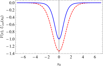
Figure 1: External potentials and effective external potentials as given by Eqs. (25) and (26), (a) with bright soliton, $g_{2}=1$, and (b) with dark soliton, $g_{2}=-1$. Solid blue and Dashed red curves correspond to the external potential and effective potential, respectively. Parameters used are: $V_{0}=1,\,g_{1}=1/2,\,n=2$.

In the following two subsections we investigate further the quantum reflection of a potential barrier both numerically and analytically. Specifically, we will show that, similar to bright solitons, sharp transition between full transmission and full reflection takes place at a critical soliton speed. The physics of quantum reflection turns out to be also similar to that of the bright soliton case where a trapped mode being formed at the potential. The critical speed for quantum reflection in terms of the strength of the potential $V_{0}$ will be also calculated using the numerical usa8 and analytical approaches.

III.1.1 Calculation of the critical speed from the numerical solution of Eq. (12)

We solve numerically Eq. (12) in the presence of the external potential (25), where we set $\delta(x)=0$ and use $\psi_{D}(x,0)$ from Eq. (14) as an initial profile. We define the scattering coefficients as

$$R=(1/N_{D})\int_{-\infty}^{-l}(|\psi_{D}(x,t_{f})|^{2}-\rho_{\infty})\,dx,$$ (27)

$$T=(1/N_{D})\int_{l}^{\infty}(|\psi_{D}(x,t_{f})|^{2}-\rho_{\infty})\,dx,$$ (28)

where $N_{D}$ is defined by Eq. (II.1), $R$ and $T$ are the scattering coefficients of reflection and transmission, respectively, $l$ is a length larger than the width of the potential, and $t_{f}$ is an evolution time such that the scattered soliton is sufficiently far from the potential. Figure 2 shows a clear possibility of obtaining quantum reflection where a sharp transmission of the coefficients from complete reflectance to complete transmittance is achieved at $v=0.67$. This is confirmed by the spatio-temporal plots in Fig. 3 (a) and (b), where the two different scattering outcomes are obtained for initial soliton speeds just below and above the critical speed. The excitation of trapped mode is also verified in Fig. 4, where a snapshot shows a dark soliton at the potential centre. Higher energy trapped modes were also found for larger potential barrier strengths. However, in such a case, quantum reflections are found to be accompanied with a considerable amount of radiation, or even completely replaced by multi-soliton ejections, as indicated by Fig. 3 (c).

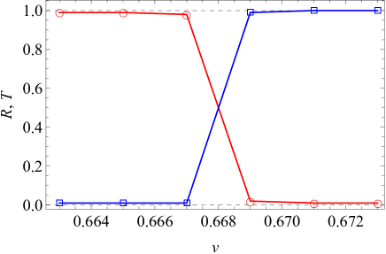
Figure 2: Reflection (red circles) and transmission (blue squares) coefficients versus initial speed of a dark soliton scattering by a reflectionless potential barrier Eq. (25). Parameters used are: $V_{0}=0.6$, $\alpha=\sqrt{V_{0}}$, $g_{1}=1/2$, $g_{2}=-1$, $x_{0}=-10$, $n=4$.

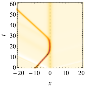
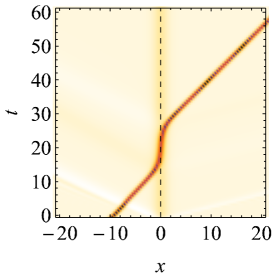
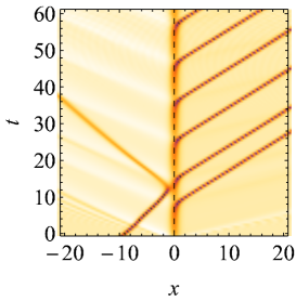
Figure 3: Quantum scattering of the dark soliton Eq. (4) by an effective potential Eq. (26). The external potential is indicated by the vertical dashed line. (a) Quantum reflection with critical speed $v=v_{c}=0.665$, (b) transmission with $v=0.67$, and (c) multi-ejection $v=0.8$, $V_{0}=2$. Other parameters used are the same of those in Fig. 2.

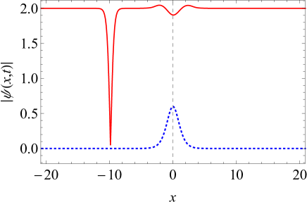
Figure 4: Existence of a trapped mode at the centre of the potential before the propagation. Dotted blue curve corresponds to the potential barrier which behaves as an effective potential well. Parameters used are: $V_{0}=0.6,\alpha=\sqrt{V_{0}},\,g_{1}=1/2,\,g_{2}=-1,\,n=4,v=0.51$.

The dependence of the critical speed for quantum reflection on the strength of the potential is shown by the solid blue curve in Fig. 5. For $V_{0}>1.1$, the scattering of dark solitons results in the above-mentioned multi-soliton ejection behaviour as illustrated in Fig. 3(c). Hence, we restricted ourselves within the goal of investigating quantum reflection while the multi-soliton ejection will be considered for the study in near future.

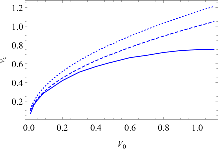
Figure 5: Critical soliton speed, $v_{c}$, at which the dark soliton will be reflected by the effective potential (26) in terms of its strength, $V_{0}$. Solid curve is obtained from the numerical solution of Eq. (12), as explained in the text. Dashed curve is the analytical result (32). Dotted curve is the result of time-dependent variational calculation (43). Parameters used are: $\alpha=\sqrt{V_{0}}$, $g_{1}=1/2$, $g_{2}=-1$, $x_{0}=-10$, $n=4$.

III.1.2 Calculation of the critical speed with exact trapped mode solution

Based on our understanding to the mechanism of quantum reflection, a trapped mode plays a crucial role in determining the sharp transition between full transmission and full (quantum) reflection. Simply, if the energy of the incoming soliton is larger (less) than the energy of the trapped mode, the soliton will be fully transmitted (reflected). If the energy of the incident soliton is equal to that of the trapped mode, the soliton will be trapped, though such a trapped state is unstable against small perturbations in position or width of the soliton. Consequently, determining the properties of the trapped mode, mainly its profile and energy, are essential for accounting to the critical speed theoretically. Fortunately, an analytic exact solution, which is the nodeless trapped mode, exists for the NLSE with the reflectionless Pöschl-Teller potential. Here, we will exploit this solution to present an analytic derivation of the critical speed in terms of the potential strength which will provide an independent account for our earlier numerical calculation which we can compare with.

In the absence of the $x$-dependent dispersion and with the presence of the Pöschl-Teller potential, $V(x)=V_{0}\,{\rm sech}^{2}(\sqrt{V_{0}}x),$ the NLSE (12) with $g_{1}=1/2$, $g_{2}<0$, and $V_{0}>0$ admits the exact dark soliton solution

$$\psi_{trap}(x,t)=\sqrt{-\frac{2V_{0}}{g_{2}}}\,{\rm tanh}\left(\sqrt{V_{0}}x\right)e^{-2iV_{0}t},$$ (29)

which upon substituting in the energy functional (17) with $U_{disp}=0$ and taking in to account the corresponding shifted intensity as $\rho(x,t)+2V_{0}/g_{2}=(2V_{0}/g_{2})\,{\rm sech}^{2}(\sqrt{V_{0}}x)$, gives the exact trapped energy that takes the form

$$E_{trap}=\frac{2V_{0}^{3/2}}{3g_{2}}.$$ (30)

The initial profile of the soliton is taken as the exact dark soliton of the fundamental NLSE, namely (4), thus the energy of the initial soliton takes the form of (7). Equating the two energies in (7) and (30), $E_{D}=E_{trap}$, yields the exact critical speed for quantum reflection

$$v_{c}=\sqrt{\frac{g_{2}^{2}n^{2}}{12}-\frac{4V_{0}^{3/2}}{3ng_{2}}}.$$ (31)

In addition to equating their energies, the norms of the initial and trapped solitons should be equal. As given by (II.1), the norm of the initial soliton is $-n$. The norm of the trapped mode (29) is calculated to be $n=4\sqrt{V_{0}}\,/g_{2}$. Equating the two norms and then substituting for $n$ in Eq. (31), we get

$$v_{c}=\sqrt{V_{0}}.$$ (32)

This theoretical result agrees favourably with the numerical calculation, as shown by dashed blue curve in Fig. 5, especially for smaller values of $V_{0}$. As noted above, for larger values of $V_{0}$, radiation increases and keeping in mind that the theoretical calculation of $v_{c}$ does not take into account radiated energy, this explains the increased deviation of the theoretical result from the numerical one.

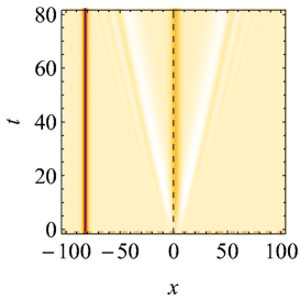
Figure 6: Numerical experiment portraying the trapped mode soliton formed at the center of the potential barrier for a stationary dark soliton positioned at $x_{0}=-80$. The external potential is indicated by the vertical dashed line. Parameters used are: $u_{0}=0.45$, $g_{1}=1/2,\,g_{2}=-1,\,V_{0}=0.1$, $\alpha=\sqrt{V_{0}}$.

Furthermore, it is observed that radiation is emitted during the population of the trapped mode even for a stationary dark soliton and irrespective of its initial position from the potential. One of such trapped mode solitons appears at the center of the potential barrier, for an initial stationary dark soliton positioned at $x_{0}=-80$, as displayed in Fig. 6. This trapped mode soliton is obtained for the initial dark soliton with an amplitude $u_{0}=\sqrt{\frac{-2V_{0}}{g_{2}}}=0.45$ using the parameter setting, $V_{0}$ = 0.1, $g_{1}$ = 0.5 and $g_{2}=-1$. Although, the exact trapped mode soliton does not account for the radiation, however, in real situations such interactions are featured with background radiation that appears on either side of the potential barrier. The emergence of such radiations is due to the continuous interaction between the background of the dark soliton with the potential barrier.

III.2 Effective position-dependent dispersion

As an alternative method of achieving quantum reflection with dark solitons, we consider a different approach that can induce the same effect of an external potential. This involves the scattering of a dark soliton by an $x$-dependent dispersion. Such $x$-dependent dispersion can be assumed as any of the following forms of $\delta(x)$:

$$U_{0}\,\delta_{Dirac}(x/w),$$ (33a)

$$U_{0}\,\times\left\{\begin{array}[]{ll}1,\hskip 14.22636pt|x|\leq w/2,\\ 0,\hskip 14.22636pt|x|>w/2,\end{array}\right.$$ (33d)

$$U_{0}\,{\rm sech}(\alpha x),$$ (33e)

$$U_{0}\,{\rm sech}^{2}(\alpha x).$$ (33f)

where $U_{0}$ and $w$ are the strength and width of the localised dispersion, respectively, and $\alpha=\sqrt{|U_{0}|}$. The effective potentials corresponding to these dispersion functions for the bright and dark solitons are calculated using Eq. (19) as

$$\frac{g_{1}nU_{0}w\alpha^{3}\,{\rm sech}^{4}(\alpha x_{0})}{4}[3-{\rm cosh}(2\alpha x_{0})],$$ (34a)

$$\frac{g_{1}nU_{0}\alpha^{2}}{6}\left\{{\rm tanh}\left[\frac{\alpha}{2}(w-2x_{0})\right]+{\rm tanh}\left[\frac{\alpha}{2}(w+2x_{0})\right]\right\},$$ (34b)

$$\pm\frac{g_{1}n\pi U_{0}\alpha^{2}}{8}{\rm sech}^{4}\left(\frac{\alpha x_{0}}{2}\right),$$ (34c)

$$\frac{g_{1}nU_{0}\alpha^{2}x_{0}\,{\rm csch}^{5}\left(\alpha x_{0}\right)}{6}\left[27{\rm sinh}\left(\alpha x_{0}\right)+7{\rm sinh}\left(3\alpha x_{0}\right)-45\alpha{\rm cosh}\left(\alpha x_{0}\right)-3\alpha{\rm cosh}\left(3\alpha x_{0}\right)\right],$$ (34d)

where in the third line, the $+$ sign relates to the effective potential for the bright soliton and the $-$ sign corresponds to the dark soliton. For the other results, the effective potential is the same for both bright and dark solitons. In Fig. 7, we plot the effective dispersion potentials obtained above for both, the bright and dark solitons.

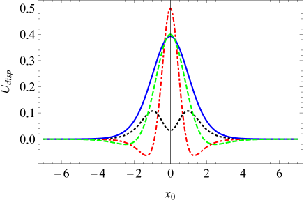
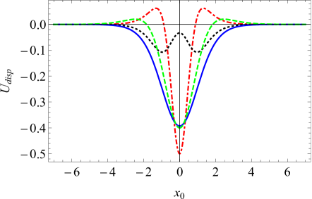
Figure 7: Effective dispersion potentials for different $x$-dependent dispersion functions $\delta(x)$, as given by Eq. (33). Dotted dashed red: Eq. (34a), Dotted black: Eq. (34b), Solid blue: Eq. (34c), Dashed green: Eq. (34d). (a) with bright soliton, $g_{2}=1$, and (b) with dark soliton, $g_{2}=-1$. Parameters used are: $U_{0}=1,\,g_{1}=1/2,\,n=2,\,w=1$.

Since the profile of the effective dispersion corresponding to $\delta(x)=U_{0}\,{\rm sech}(\alpha x)$ has monotonically-decaying tails and without the appearance of pedestals besides the main peak, we select to focus on this function through our investigations below. Additionally, pulse profiles featured with pedestals result in complex scattering dynamics and eventually lead to some further radiation during the numerical simulations. A similar analogy to the case with external potential applies here; for dark solitons, quantum scattering requires the effective potential to be a well. Thus, quantum scattering can be achieved with the parameter set $g_{1}>0$, $g_{2}<0$, $U_{0}>0$, while the parameter set $g_{1}>0$, $g_{2}<0$, $U_{0}<0$, leads to the classical scattering regime.

In the following, we discuss the results obtained for quantum scattering parameters. We solve numerically Eq. (12) using the function (33e). We set $V(x)=0$ and launch $\psi_{D}(x,0)$ using Eq. (12) as an initial soliton. We defined the reflection and transmission coefficients by Eqs. (27) and (28), where in this situation, $l$ indicates the length larger than the width of the $x$-dependent dispersion. In Fig. 8, we plot the scattering coefficients versus the incident soliton speed. The figure clearly shows the possibility of obtaining quantum reflection, where a sharp transmission of the coefficients from full reflectance to full transmittance is achieved. This is confirmed by the spatio-temporal plots in Fig. 9. The critical speed for quantum reflection, $v_{c}$, is calculated numerically by running the initial soliton speed such that it gets trapped at the potential. In Fig. 10, we plot the critial speed versus $U_{0}$. The dependence of $v_{c}$ on $U_{0}$ is found to be similar to that of dependence of $v_{c}$ on $V_{0}$ for the the external potential barrier case. Moreover, in Fig. 9 (c), we show a multi-ejection behavior for the larger values of $U_{0}$, as the one observed for the external potential barrier.

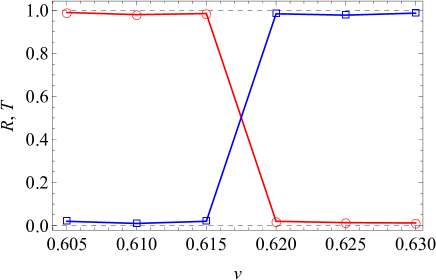
Figure 8: Reflection (red circles) and transmission (blue squares) coefficients versus initial speed of a dark soliton scattering by an $x$-dependent dispersion (33e). Parameters used are: $U_{0}=0.4$, $g_{1}=1/2$, $g_{2}=-1$, $\alpha=\sqrt{g_{1}U_{0}}$, $x_{0}=-10$, $n=-4$.

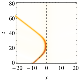
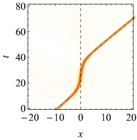
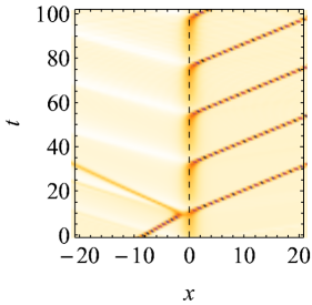
Figure 9: Quantum scattering of the dark soliton (4) by an $x$-dependent dispersion (33e). The centre of the $x$-dependent dispersion is indicated be the vertical dashed line. (a) Quantum reflection with critical speed $v=v_{c}=0.615$, (b) transmission with $v=0.62$, and (c) multi-ejection $v=0.8$, $U_{0}=2$. Parameters used are the same of those in Fig. 8.

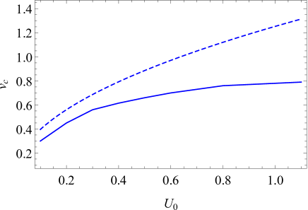
Figure 10: Critical soliton speed, $v_{c}$, at which the dark soliton will be reflected by the $x$-dependent dispersion (33e) in terms of its height, $U_{0}$. Solid curve is obtained from the numerical solution of Eq. (12), as explained in the text. Dashed curve is the result of time-dependent variational calculation (47). Parameters used are: $g_{1}=1/2$, $g_{2}=-1$, $\alpha=\sqrt{g_{1}U_{0}}$, $x_{0}=-10$, $n=4$.

IV Scattering dynamics of dark solitons using time-dependent variational calculations

In this section we use a time-dependent variational calculation to obtain an analytical account of the dynamical evolution of the scattering soliton. The appearance of quantum reflection above a critical speed will be then confirmed. This will also provide analytical expressions of the critical speed for both cases of external potential and position-dependent dispersion.

We employ the trial function of the dark soliton in (9) with varying the soliton centre and velocity in $t$ and the use of the shifted intensity, namely, $v\rightarrow v(t)$, $x_{0}\rightarrow x_{0}(t)$, and $\rho(x,t)=-(n\alpha/2)\,{\rm sech}^{2}[\alpha(x-x_{0}(t))]$.

The Lagrangian function corresponding to the NLSE, Eq. (12), then takes the form

$$L = \int_{-\infty}^{\infty}i\psi^{*}(x,t)\psi_{t}(x,t)dx-\int_{-\infty}^{\infty}\left[g_{1}|\psi_{x}(x,t)|^{2}-\frac{1}{2}g_{2}|\psi(x,t)|^{4}+V(x)|\psi(x,t)|^{2}\right]dx$$ (35)

$$= \int_{-\infty}^{\infty}i\psi^{*}(x,t)\psi_{t}(x,t)dx-\left[E_{0}+U_{disp}(x_{0},v)+U_{ext}(x_{0},v)\right],$$

where we have hidden the $t$-dependence for convenience.

IV.1 Effective external potential well

In the presence of external potential barrier and with the absence of the $x$-dependent dispersion, $V(x)=V_{0}\,{\rm sech}^{2}(\alpha x)$, $\delta(x)=0$, the calculated Lagrangian in (35) with the trial function of the dark soliton, (9), takes the form

$$L = -nv\dot{x_{0}}-\left\{-\frac{1}{3}g_{1}n(\alpha^{2}+3v^{2})-\frac{1}{6}g_{2}n^{2}\alpha-2nV_{0}{\rm csch}^{2}(\alpha x_{0})\left[\alpha x_{0}{\rm coth}(\alpha x_{0})-1\right]\right\}.$$ (36)

The corresponding Euler-Lagrange equations yield the following two equations of motion for the soliton centre and velocity

$$\dot{x_{0}}-2g_{1}v=0,$$ (37)

$$-n\dot{v}-6nV_{0}\alpha{\rm coth}(\alpha x_{0}){\rm csch}^{2}(\alpha x_{0})+2V_{0}\alpha^{2}x_{0}(t){\rm csch}^{4}(\alpha x_{0})\,[2+{\rm cosh}(2\alpha x_{0})]=0.$$ (38)

Integrating the above equation with respect to $x_{0}$ results in

$$-2nV_{0}{\rm csch}^{2}(x_{0})[\alpha{\rm coth}(\alpha x_{0})x_{0}-1]-\frac{1}{2}nv^{2}-c=0,$$ (39)

where $c$ is the constant of integration.

For an initial position, $x_{0}(0)$, that is sufficiently far from the influence of the potential $V(x)$, the constant of integration can be calculated as

$$c=\frac{-nv_{c}^{2}}{2},$$ (40)

where $v_{c}=v(0)$.

Substituting the obtained constant of integration in (39) leads to

$$-2nV_{0}\,{\rm csch}^{2}(x_{0})[\alpha\,x_{0}\,{\rm coth}(\alpha x_{0})-1]+\frac{1}{2}n(v^{2}-v_{c}^{2})=0.$$ (41)

At the turning point which takes place at $t=t_{c}$, the velocity of the dark soliton vanishes, $v(t_{c})=0$ and thus $v_{c}$ can be calculated from from the last equation as

$$v_{c}=-2\sqrt{V_{0}}\left(\sqrt{\left\{x_{0}(0)\,\alpha\,{\rm coth}[x_{0}(0)\,\alpha]-1\right\}}\,{\rm csch}[x_{0}(0)\,\alpha]\right).$$ (42)

The turning point position, $x_{0}(0)$, can be calculated from Eq. (38) by setting the effective force to zero, namely $n\dot{v}=0$, which gives the solution $x_{0}(0)=0$. Direct substitution of $x_{0}(0)=0$ in the last equation leads to an undefined quantity. However, expanding it in powers of $x_{0}(0)$ and then taking the limit $x_{0}(0)\rightarrow 0$, shows that all terms except the zeroth order one, vanish, and the result becomes

$$v_{c}=2\sqrt{\frac{V_{0}}{3}}.$$ (43)

This result is plotted by the dotted blue curve in Fig. (5). While good agreement is obtained with the numerical values for smaller barrier heights, $V_{0}$, the deviation increases for larger barrier heights. The discrepancy is primarily due to not accounting for radiation and multi-ejection in the present variational approach.

In Fig. 11, we display the time varying position and speed obtained from the solutions of the equations of motion (37) and (38), that clearly show sharp transition from full reflection to full transmission.

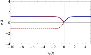
Figure 11: Dynamics of the variational parameters, speed $v(t)$ versus position $x_{0}(t)$ corresponding to NLSE with external potential, Eqs. (37) and (38). Sharp reflection (dashed red) occurs at the critical speed $v=v_{c}=1.15$ and transmission (blue) occurs at $v=1.156$. Parameters used are: $V_{0}=1,\,g_{1}=1/2,\,g_{2}=-1,\,n=4$.

IV.2 Effective well with position-dependent dispersion

In the presence of position-dependent dispersion given by $\delta(x)=U_{0}\,{\rm sech}(\alpha x)$ and with $V(x)=0$, the calculated Lagrangian in (35) with the trial function of the dark soliton, (9), is reduced to

$$L = -nv\dot{x_{0}}-g_{1}\left[-\frac{1}{3}n\alpha^{2}-\frac{\pi}{4}nU_{0}v^{2}{\rm sech}^{2}\left(\frac{1}{2}\alpha x_{0}\right)-\frac{\pi}{8}nU_{0}\alpha^{2}{\rm sech}^{4}\left(\frac{1}{2}\alpha x_{0}\right)-nv^{2}-\frac{1}{6g_{1}}g_{2}n^{2}\alpha\right],$$ (44)

where, based on our earlier discussion, we have neglected the nonhermitian term. The Euler-Lagrange equations yield the following two equations of motion for the soliton centre and velocity

$$n\dot{x_{0}}-2g_{1}nv-\frac{\pi}{2}g_{1}nvU_{0}{\rm sech}^{2}\left(\frac{1}{2}\alpha x_{0}\right)=0,$$ (45)

$$-n\dot{v}+\frac{\pi}{4}g_{1}n\,\alpha\,U_{0}{\rm sech}^{2}\,\left(\frac{1}{2}\alpha x_{0}\right){\rm tanh}\left(\frac{1}{2}\alpha x_{0}\right)\left[v^{2}+\alpha^{2}{\rm sech}^{2}\left(\frac{1}{2}\alpha x_{0}\right)\right]=0.$$ (46)

Following the derivation of $v_{c}$ expression (43) in the previous section, we obtain the critical speed for the present case

$$v_{c}=\frac{1}{2}\alpha\sqrt{\pi g_{1}U_{0}}.$$ (47)

The comparative results for $v_{c}$ obtained through Lagrangian approach and those through numerical simulations are shown in Fig. 10. Similar to the previous case, deviation of the variational values from the numerical ones increase with increasing $U_{0}$, which, as we explained above is due not accounting for radiation. The trajectory in this case turns out to be very similar to that in Fig. 11 confirming the critical scattering behaviour.

V conclusions and outlook

We have considered quantum reflection of dark solitons in two setups, (i) in the presence of external potentials and (ii) in the presence of an $x$-dependent dispersion. At the outset, we have revisited the energy calculations and normalization of both bright and dark solitons in order to determine the energy functional and the condition that is necessary for quantum reflection to occur with dark solitons. Both analytical and variational calculations have shown that for quantum reflection of dark solitons to occur in the aforementioned setups, the actual external potential or dispersion modulation need to be a barrier-like function which leads to an effective potential well in both cases.

In order to investigate the scattering dynamics, we have derived the effective external potential corresponding to an external potential and an $x$-dependent dispersion using a suitable trial function for the dark soliton pulse. In the presence of an external potential, we have considered the reflectionless Pöschl-Teller potential and for $x$-dependent dispersion we used the ‘sech’ function, owing to its corresponding effective potential without pedestals. This is followed by the numerical and analytical study of the soliton scattering.

Through our numerical investigations, we have observed quantum reflection for dark solitons for both settings considered. The critical speed required for such phenomenon tends to increase with the height of the barrier. Moreover, our study revealed a transition regime from clear quantum reflection to a multi-ejection behaviour for larger barrier heights. Analytical calculation of the critical speed in the case of external potential was also possible using the exact trapped mode profile of the dark soliton scattered by a reflectionless potential barrier.

Then, we have derived the relation for the critical speed using variational calculations for the two setups considered. The variational study has successfully shown the sharp transition behavior from full reflection to full transmission at the critical speed. The deviation of the critical speed values calculated by the exact trapped mode or by the variational calculation from the exact numerical ones increases for larger potential strengths. This is due to not including radiation in the analytical calculation. While the inclusion of radiation complicates the calculations, we believe it is worth investigating in a future work, as this will result in an accurate analytical formula that predicts the threshold of quantum reflection.

The above study is fully oriented to the quantum reflection, but in general such interactions lead to many other interesting phenomena such as multi-ejection, snake trapping, and tree-ejection which are possible by controlling the system parameters. In particular, we have noticed a region in the parameters space where periodic ejection of dark solitons is stimulated by the scattering. This behavior will be considered in near future.

References

- (1) C. Lee and J. Brand, Europhys. Lett. 73, 321 (2006).
- (2) T. Ernst and J. Brand, Phys. Rev. A. 81, 033614 (2010).
- (3) U. Al Khawaja, Phys. Rev. E 103, 062202 (2021).
- (4) T. Uthayakumar, L. Al Sakkaf, and U. Al Khawaja, Phys. Rev. E 104, 034203 (2021).
- (5) H. Sakaguchi and M. Tamura, J. Phys. Soc. Jpn. 74, 292 (2005).
- (6) C. Weiss and Y. Castin, Phys. Rev. Lett. 102, 010403 (2009).
- (7) O. V. Marchukov, B. A. Malomed, V. A. Yurovsky, M. Olshanii, V. Dunjko, and R. G. Hulet, Phys. Rev. A 99, 063623 (2019).
- (8) V. Dunjko, M. Olshanii, arXiv:1501.00075v4 (2020).
- (9) A. E. Miroshnichenko, S. Flach, and B. Malomed, Chaos 13, 874 (2003).
- (10) K. T. Stoychev, M. T. Primatarowa, and R. S. Kamburova Phys. Rev. E 70, 066622 (2004).
- (11) M. Lizunova, O. Gamayun, arXiv:2010.03385 (nlin), (2010).
- (12) Y. Nogami and F.M.Toyama, Phys. Lett. A 184, 245 (1994).
- (13) F. Baronio, C. De Angelis, P. Pioger, V. Couderc, and A. Barthélémy, Opt. Lett. 29, 986 (2004).
- (14) H. Friedrich and J. Trost, Phys. Rep. 397, 359 (2004).
- (15) R. Cote, H. Friedrich, and J. Trost, Phys. Rev. A 56, 1781 (1997).
- (16) M. Asad-uz-zaman and U. Al Khawaja, EPL 101, 50008 (2013).
- (17) U. Al Khawaja, S. M. Al-Marzoug, H. Bahlouli, and Y. S. Kivshar, Phys. Rev. A 88, 023830 (2013).
- (18) M. O. D. Alotaibi, S. M. Al-Marzoug, H. Bahlouli, and U. Al Khawaja, Phys. Rev. E 100, 042213 (2019).
- (19) U. Al Khawaja and Andery A. Sukhorukov, Opt. Lett. 40, 2719 (2015).
- (20) U. Al Khawaja, S. M. Al-Marzoug, and H.Bahlouli, Phys. Lett. A 384, 126625 (2020).
- (21) A. Javed, T. Uthayakumar, M. O. D. Alotaibi, S. M. Al-Marzoug, H. Bahlouli, and U. Al Khawajaa, Commun. Nonlinear Sci. Numer. Simulat. 103, 105968 (2021).
- (22) G. P. Agrawal, Nonlinear Fiber Optics, Academic Press, 2013. ISBN: 9780123970237.
- (23) G. P. Agrawal, Fiber-Optic Communication Systems, Wiley, 2010. ISBN: N 9780470505113.
- (24) U. Al Khawaja, and L. Al Sakkaf, Handbook of Exact Solutions to the Nonlinear Schrödinger Equations, IOP Publishing Ltd 2020, London. Online ISBN: 978-0-7503-2428-1, Print ISBN: 978-0-7503-2426-7.
- (25) U. Al Khawaja and Q. M. Al-Mdallal, Int. J. Diff. Eq. 2018, 6043936 (2018); L. Al Sakkaf, Q. M. Al-Mdallal, and U. Al Khawaja, Complexity 2018, 8269541 (2018); L. Al Sakkaf and U. Al Khawaja, arXiv:2108.00936.
- (26) A. Hasegawa and F. Tappert, Appl. Phys. Lett. 23, 171 (1973).
- (27) D. Krökel, N. J. Halas, G. Giuliani, and D. Grischkowsky, Phys. Rev. Lett. 60, 29 (1988).
- (28) Y. S. Kivshar and B. Luther-Davies, Phys. Rep. 298, 81 (1998).
- (29) A. M. Weiner, J. P. Heritage, R. J. Hawkins, R. N. Thurston, E. M. Kirschner, D. E. Leaird, and W. J. Tomlinson, Phys. Rev. Lett. 61, 2445 (1988).
- (30) E. Smirnov, C. E. Rüter, M. Stepic, D. Kip, and V. Shandarov, Phys. Rev. E. 74, 065601(R) (2006).
- (31) A. Chabchoub, O. Kimmoun, H. Branger, N. Hoffmann, D. Proment, M. Onorato, and N. Akhmediev, Phys. Rev. Lett. 110, 124101 (2013).
- (32) M. Chen, M. A. Tsankov, J. M. Nash, and C. E. Patton, Phys. Rev. Lett. 70, 1707 (1993).
- (33) D. J. Frantzeskakis, J. Phys. A: Math. Theo. 43, 213001 (2010).
- (34) R. Heidemann, S. Zhdanov, R. Sütterlin, H. M. Thomas, and G. E. Morfill, Phys. Rev. Lett. 102, 135002 (2009).
- (35) P. Emplit, J. P. Hamaide, F. Reynaud, C. Froehly, and A. Barthélémy, Opt. Commun. 62, 374 (1987).
- (36) S. A. Gredeskul and Yu. S. Kivshar, Opt. Lett. 14, 1281 (1989).
- (37) Q. Cheng, W. Bai, Y. Zhang, B. Xiong, and Tao Yang, Laser Phys. 29, 015501 (2018).
- (38) M. Sciacca, C. F. Barenghi, and N. G. Parker, Phys. Rev. A 95, 013628 (2017).
- (39) F. Tsitoura, Z. A. Anastassi, J. L. Marzuola, P. G. Kevrekidis, and D. J.Frantzeskakis, Phys. Lett. A 381, 2514 (2017).
- (40) Z. Deng, Y. Chen, J. Liu, C. Zhao, and D. Fan, Opt. Lett. 43, 5327 (2018).
- (41) M. O. D. Alotaibi and L. D. Carr, J. Phys. B: At. Mol. Opt. Phys. 52, 165301 (2019).
- (42) S. D. Hansen, N. Nygaard, and K. Mølmer, Appl. Sci. 11, 2294 (2021).