Microdosing: Knowledge Distillation for GAN based Compression

Abstract

Recently, significant progress has been made in learned image and video compression. In particular, the usage of Generative Adversarial Networks has led to impressive results in the low bit rate regime. However, the model size remains an important issue in current state-of-the-art proposals, and existing solutions require significant computation effort on the decoding side. This limits their usage in realistic scenarios and the extension to video compression. In this paper, we demonstrate how to leverage knowledge distillation to obtain equally capable image decoders at a fraction of the original number of parameters. We investigate several aspects of our solution including sequence specialization with side information for image coding. Finally, we also show how to transfer the obtained benefits into the setting of video compression. Altogether, our proposal allows to reduce a decoder model size by a factor of 20 and to achieve 50% reduction in decoding time.

1 Introduction

Initially, projections for 2022 have estimated that video content would reach 82% of internet traffic. While this would already make video the most prevalent form of media in terms of bandwidth by far, the current pandemic situation pushed video traffic even further than these expectations due to the need for social distancing and home officing (NYTimes, 2020). As a result, compression techniques are more challenged than ever to handle visual data efficiently, and improvements can impact the daily lives of millions of people.

In contrast to the hand-crafted individual components of traditional codecs, learned image compression schemes aim to learn an optimal non-linear transform from data, ideally in an end-to-end fashion. At a high level, most of the methods can be understood as a sort of generative model that tries to reconstruct the input instance from a quantized latent representation, coupled with a prior that is used to compress these latents losslessly (Ballé et al., 2017). Although providing good perceptual quality in the high bitrate target setting, it is the low bitrate setting in which neural image compression has shown most of its strength. In particular, GAN (Generative Adversarial Networks)-based architectures for image compression (Agustsson et al., 2019; Mentzer et al., 2020) are able to produce impressive results by generating an appropriate hallucination of detail in the output image. As a drawback, GAN-based compression frameworks usually have large decoder models that are many times trained on private datasets. Therefore, retraining these models to their original performance is not generally possible, and even if the data was present, it would not be straightforward and time consuming. In addition, the memory requirements and inference time make them less practical, especially in the context of video coding and mobile devices.

This paper proposes a knowledge distillation (KD) (Beyer et al., 2021) approach that allows retaining good perceptual image quality while reducing the size of the decoder. The goal of KD is to transfer the learned knowledge of a teacher network on a smaller student network that remains competitive to the teacher network performance. By requiring less memory and computational power than the initial teacher network, the student network could, for instance, run on less powerful devices such as mobile phones or dedicated devices. Being able to compress the generator network or decoder in the auto-encoder setting is not only interesting in terms of memory requirements but also in terms of computational efficiency. This is especially important for image and video compression, where the majority of the computation should preferably be on the sender (encoder) side, while the decoding should be simple. Especially in the context of video streaming, an asset will typically be encoded once while it will be distributed and decoded millions of times. Traditional codecs do spend a lot of emphasis and compute on encoding while keeping decoding extreme lightweight. In contrast to that, deep learning based architectures are typically symmetric in terms of encoding and decoding or can even require considerably more compute for decoding when using a GAN (Mentzer et al., 2020).

Our proposal is based on: i) training a reduced student decoder with data generated from the big decoder. ii) overfitting the reduced student decoder model to a specific image or set of images; and iii) sending the specialized decoder weights alongside the image latents. To show the viability of our proposal, we incorporate it into state-of-the-art models for neural image and video compression targeting the low bitrate setting. First, we replace the High-Fidelity Compression (HiFiC) (Mentzer et al., 2020) decoder with a much smaller student decoder. HiFiC is the state-of-the-art in low bitrate neural image compression (~0.15 bpp) that produces extremely competitive results at the cost of a fairly big (~156M parameters) decoder network. Our proposed KD approach allows for a much smaller decoder (~8M parameters) and 50% faster decoding time while still producing visually similar output images. Second, we show how to apply our KD strategy in a neural video compression framework based on latent residuals (Djelouah et al., 2019b). In such a scenario, we overfit our reduced student decoder to a sequence so that we can provide a sequence specific decoder. We show that the additional bits needed for sending the weights amortize over the sequence.

Explicitly, the main contributions of this paper are: i)  proposing novel strategies for KD for neural image and video compression; ii) investigating KD in the low bitrate setting for GAN-based image compression; iii) investigating KD in the low bitrate GAN-based video compression setting with latent residuals.

2 Related Work

Neural image compression

The first proposed neural image compression methods (Ballé et al., 2016; Toderici et al., 2016, 2017) showed improved results over JPEG or JPEG2000, while most recent approaches (Ballé et al., 2018; Mentzer et al., 2018; Minnen et al., 2018; Helminger et al., 2020; Choi et al., 2019) are now on par or surpassing BPG (Fab, 2015). Recent works (Patel et al., 2019b, 2021, a; Hepburn et al., 2021) also investigate the application of perceptual losses and how they relate to the human visual perception of decompressed images.

In particular, generative methods have been providing impressive results in the low bitrate setting (Agustsson et al., 2019; Mentzer et al., 2020). Generative models for image compression are able to synthesize details that would be very costly to store, resulting in visually pleasing results at bitrates in which previous methods show strong artifacts (Agustsson et al., 2019). However, to synthesize those details, a powerful and potentially big decoder is necessary, which contradicts the general requirements on compression technologies, where the sender (encoder) should have the burden of computing a good compression, such that the receiver (decoder) can be as simple as possible. Our approach can be applied to any of the neural image compression methods above, whenever the decoder is too big and faster inference times are required. This is especially crucial in GAN-based neural compression methods. As a use case, we show an application of our proposal using HiFiC (Mentzer et al., 2020), which is the state-of-the-art GAN model for low bit rate image compression.

Neural video compression

As an extension to the neural image compression methods, neural video compression approaches aim to leverage redundancy in both spatial and temporal information. (Lu et al., 2019b) replace blocks in traditional video codecs with neural networks. Learning-based optical flow estimation is used to obtain the motion information and to reconstruct the current frames. Then they employ two auto-encoder networks to compress the corresponding motion and residual information. Veerabadran et al. (2020) show that minimizing an auxiliary adversarial distortion objective for neural video compression in the low bitrate setting creates distortions that better correlate with human perception. Djelouah et al. (2019b) propose compressing and sending residuals in the latent space instead of residuals in the pixel space, which allows the reuse of the same image compression network for both keyframes and intermediate frames. In this paper, we use such an approach as a starting point to show the viability of KD in neural video compression. Instead of explicitly computing residuals or differences, Ladune et al. (2021) use feature space concatenation and train a decoder that operates on this joint information. van Rozendaal et al. (2021) present an extreme approach that fine tunes the full model to a single video, and sends model updates (quantized and compressed using a parameter-space prior) along with the latent representation. Such an approach is in line with our idea of sequence-specific information to be sent to the student decoder, and our work can be seen as complementary to (van Rozendaal et al., 2021), which does not include KD.

Knowledge distillation

KD has been primarily used on vision tasks like object classification or segmentation. KD for generative models, however, is not well studied yet. In (Chang and Lu, 2020), the authors leveraged a teacher-student architecture to reduce the size of the BigGAN (Brock et al., 2018) architecture while still being competitive on Inception and FID scores. To the best of our knowledge, our work is the first to propose knowledge distillation to learn a smaller decoder for neural image and video compression frameworks.

3 Knowledge Distillation for Compression

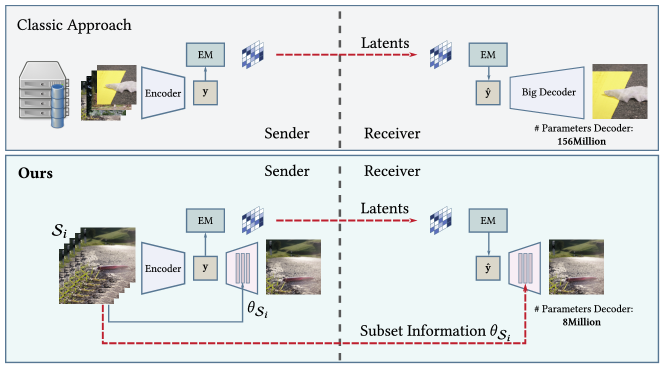
Figure 1 illustrates an overview of our proposal. In the classic neural compression approach, the encoder-decoder pair is trained on a big dataset, to get an overall good performance on a variety of different content. Once the auto-encoder is fully trained, the decoder gets deployed and sent to the receiver. The potentially big decoder then allows to decode any type of content. In our approach, we enable the sender to partition the data into subsets $\mathcal{S}_{i}$, and learn a content-specific decoder with corresponding information $\theta_{\mathcal{S}_{i}}$ for each subset. This specialization allows us to train a model with less parameters, smaller memory footprint, and less computations. Once the decoder is fully trained, and the sender’s reconstruction quality requirement of the subset is fulfilled, the content-specific information is stored alongside the subset. If the receiver wants to decode an image $\mathbf{x}\in\mathcal{S}_{i}$, the subset specific information $\theta_{\mathcal{S}_{i}}$ has to be sent once per subset. Next, we detail how to apply our distillation process to image compression with GANs and extend this to video compression using latent space residuals.

Figure 1: Overview of our proposal: we replace the Big Decoder of GAN compression models (top) with a smaller decoder plus a content-specific additional information (bottom).

3.1 Knowledge Distillation for Image Compression with GANs

High-Fidelity Generative Image Compression (HiFiC)

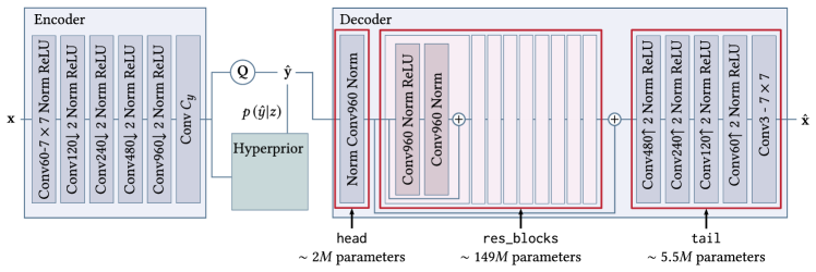
Figure 2 shows the HiFiC architecture (Mentzer et al., 2020) . Its decoder can be divided into three sub-nets: head (~2M parameters), res_blocks (~149M parameters), and tail (~5.5M parameters). Through experimentation, and as shown in Figure 3, it is easy to conclude that the coarse information of the image is saved in the latent space, and the hallucination of the texture is generated by the residual network (res_blocks) of the decoder. In particular, the discrepancy in size of the the res_blocks is due to the fact that the model was trained on a big (private) dataset, thus such a big size is needed to capture all the textures seen during training. However, if we know in advance which images should be compressed (e.g. frames of a video with similar features), we can overfit to this data and sent only the necessary weights to properly decode these images. That is exactly what we propose with the Distilled-HiFiC architecture bellow.

Figure 2: Architecture of High-Fidelity Generative Image Compression (HiFiC)

(a) $\text{\emph{HiFiC}}^{Lo}$

(b) $\text{\emph{HiFiC}}^{Lo}$ (w/o RB)

(c) $\text{\emph{HiFiC}}^{Hi}$

(d) $\text{\emph{HiFiC}}^{Hi}$ (w/o RB)

Figure 3: Even without residual blocks (RB), the HiFiC model outputs a coarse version of the image. The images show the output of HiFiC models with (a), (c) and without (b), (d) residual blocks.

(a) Teacher-Student Architecture

(b) Micro-RN

Figure 4: Visualization of the proposed Micro-RN. If not stated explicitly, a $3\times 3$ convolution is used. DConv denotes a depthwise convolution and $C_{h}$ is the number of hidden channels.

Distilled-HiFiC

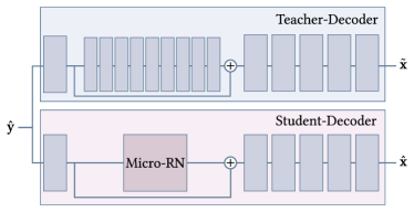
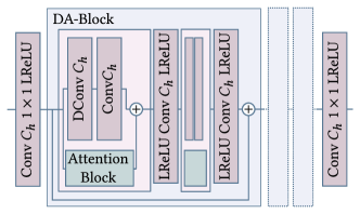
Our proposed Distilled-HiFiC (See Figure 4a) reduces the size of the decoder by training a smaller sub-network, named Micro-Residual-Network (Micro-RN) that mimics the behavior of the residual network (res_blocks) for a specific subset, and therefore microdosing the capability of hallucinations. Micro-RN is based on the degradation-aware (DA) blocks introduced in (Wang et al., 2021). While (Wang et al., 2021) utilizes a kernel prediction network to steer the weights according to a degradation vector, we learn a set of weights $\theta_{\mathcal{S}_{i}}$ per subset $\mathcal{S}_{i}$. Micro-RN is defined by two parameters: $C_{h}$, the number of hidden channels, and $B$, the number of DA Blocks. Similar as in (Chang and Lu, 2020), we train Micro-RN with the teacher-student architecture (Figure 4a), with the difference that our decoder borrows pre-trained layers (i.e., head and tail) from the teacher-decoder. Let $\mathbf{x}\in\mathcal{S}_{i}$ be an image of subset $\mathcal{S}_{i}$ and $\tilde{\mathbf{x}}$ be the image compressed by the teacher network. We optimize the following loss:

$$\mathcal{L}\left(\mathbf{x};\theta_{\mathcal{S}}\right)=k_{M}\text{MSE}\left(\tilde{\mathbf{x}},\hat{\mathbf{x}}\right)+k_{p}d_{p}\left(\hat{\mathbf{x}},\mathbf{x}\right),$$ (1)

where $\hat{\mathbf{x}}$ is the output of the student network, MSE and $d_{p}$ are the distortion losses, and $k_{M}$ and $k_{p}$ are their corresponding weights. Similar to (Mentzer et al., 2020) as the perceptual loss $d_{p}=\text{LPIPS}$ (Zhang et al., 2018) is used. Hence, the loss forces the student-decoder to generate images that look similar to the teacher’s and further reduce the perceptual loss to the ground truth image. Note, that we freeze both the encoder and the entropy model which in this case is modeled using a hyperprior. Hence, $\theta_{\mathcal{S}}$ only contains the weights of the Micro-RN. This allows us to leverage the powerful encoder and hyperprior of HiFiC as well as the models knowledge about the private training data set.

3.2 Knowledge Distillation for Video Compression with Latent Space Residuals

Figure 5: Overview of knowledge distillation with latent residuals for video compression: Frame Prediction Network (FPN) and Latent Residual Network (LRN)

To show the application of KD in neural video compression scenarios, we use a similar approach as proposed by Djelouah et al. (2019a). (see Figure 5). Such network is composed of two parts: a Frame Prediction Network (FPN) and a Latent Residual Network (LRN). Given a sequence of frames (group of pictures, or GOP) to be encoded $\mathbf{x}_{0},...,\mathbf{x}_{GOP}$, where $\mathbf{x}_{0}$ is a keyframe (I-frame) and $\mathbf{x}_{1},...,\mathbf{x}_{GOP}$ are predicted frames (P-frames), the compression of the sequence works as follows:

First, the I-frame ($\mathbf{x}_{0}$) is compressed using a neural image-only compression network to generate the encoded latent $\mathbf{y}_{0}$. $\hat{\mathbf{x}}_{0}$ denotes the reconstructed frame from the quantized latent $\hat{\mathbf{y}}_{0}$. Then, for each P-frame, $\mathbf{x}_{t+1},1\leq t+1\leq GOP$, we: (1) generate a temporal prediction, $\mathbf{x}^{Pred}_{t+1}$, of $\mathbf{x}_{t+1}$ from the previous reconstructed frame, $\hat{\mathbf{x}}_{t}$, using FPN. The FPN works by first computing the optical flow $\mathbf{f}_{t+1}$ between $\mathbf{x}_{t+1}$ and $\hat{\mathbf{x}}_{t}$. (2) use the neural motion compression network to generate the encodings and quantized latents $\hat{\mathbf{w}}_{t+1}$ of $\mathbf{f}_{t+1}$. (3) warp $\hat{\mathbf{x}}_{t}$ with the decompressed flow $\hat{\mathbf{f}}_{t+1}$, and then motion compensating it to generate the temporal $\mathbf{x}^{Pred}_{t+1}$.
To compute the residual between the temporal prediction and the P-Frame, we use the LRN: (4) we encode both, the prediction $\textbf{x}^{Pred}_{t+1}$ and $\textbf{x}_{t+1}$, with $E_{I}$ (a pretrained image compression encoder) and (5) compute the latent residual, $\mathbf{r}_{t+1}$, between the latents of the P-frame against the predicted frame, $\mathbf{r}_{t+1}=\mathbf{y}_{t+1}-\mathbf{y}^{Pred}_{t+1}$, which is then quantized and entropy coded with  EM_I. The final bitstream of a GOP is then composed of $\{\hat{\mathbf{y}}_{0},\hat{\mathbf{w}}_{1},...,\hat{\mathbf{w}}_{GOP},\hat{\mathbf{r}}_{1},...\hat{\mathbf{r}}_{GOP}\}$, i.e., latent of the I-frame and the compressed flow fields and latent residuals for each of the P-frames (all quantized and entropy encoded).

In the low bitrate setting, HiFiC would seem like a suitable choice for the neural image compression architecture that could be used together with the above latent space residual framework. As previously mentioned, however, the size of the HiFiC decoder is a limiting factor. Also, inference time is even more important in the video setting that should be able to keep a decoding frame rate of ~30 frames per seconds (fps). Thus, we propose to use our Distilled-HiFiC in the latent residual framework above.

During encoding, we overfit our Distilled-HiFiC to a specific sequence so that we only need to send the $\theta_{\mathcal{S}}$ once for all the frames of that sequence. Our decoding process starts then by receiving and loading sequence-specific Micro-RN weights on the Distilled-HiFiC decoder, which is then fixed during the decode of the whole sequence. As detailed next, with such an small overhead, we can reduce the decoding time by half while keeping similar visual quality to the latent residual framework using the original HiFiC decoder.

4 Experiments

In this section we first describe the experiment that leads to the minimal architecture that is powerful to mimic HiFiC’s residual network on a variety of subsets. In the second part of this section, we show that our student decoder can be used for video compression based on latent space residuals and compare the results with OpenDVC, a recent neural video compression method.

Dataset

The models were trained on two types of subsets: $\mathcal{S}_{uvg}$ a subset of UVG (Mercat et al., 2020) and $\mathcal{S}_{i}$ a subset of sequence $i\in\{1,\dots,7\}$. We created the subsets by taking every 10th frame of each clip. This allows Micro-RN to learn the image features present in the whole clip. $\mathcal{S}_{uvg}$ consists in total of 390 frames with resolution $1920\times 1080$ and $\mathcal{S}_{i}$ of up to 60 frames.

We evaluated the proposed model for qualitative comparisons on an in-house created movie. The subset $S_{i}$ corresponds to a specific clip, where $S_{lucid}$ denotes the union of four clips.

4.1 Micro-Residual-Network

Training

We trained our Micro-RN by minimizing Equation 1 on random crops of size $256\times 256$. We used the hyper parameters $k_{p}$ and $k_{M}$ proposed in (Mentzer et al., 2020). We further used the Adam optimizer (Kingma and Ba, 2015) with a learning rate of $10^{-4}$ and batch size 4. Training a model takes approximately 10 hours on a NVIDIA Titan Xp.

Ablation Study

To find the minimum number of weights for Micro-RN, we trained our student decoder with various number of hidden channels $C_{h}=\{64,128,256\}$ and DA blocks $B=\{1,2,3,4\}$. We are interested in the smallest possible architecture that is still capable to mimic $HiFiC$’s residual network. $HiFiC^{Lo}$ is selected as the teacher network, since it is the model that has the most difficult task of hallucinating details. Table 1 shows the number of parameters per configuration.

		$C_{h}$
		64	128	256
$B$	1	211k	594k	1.88M
	2	294k	925k	3.19M
	3	378k	1.25M	4.51M
	4	461k	1.59M	5.82M

Table 1: Number of parameters per tested configuration.

Architecture

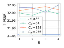
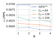
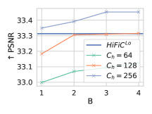
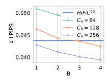
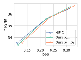
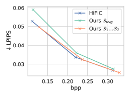
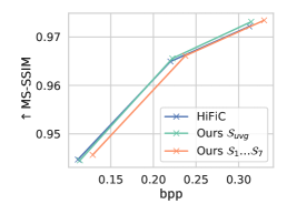
To find the minimum number of weights for Micro-RN, we trained our student decoder with various number of hidden channels $C_{h}=\{64,128,256\}$ and DA blocks $B=\{1,2,3,4\}$. We are interested in the smallest possible architecture that is still capable to mimic HiFiC’s residual network. $\text{\emph{HiFiC}}^{Lo}$ is selected as the teacher network, since it is the model that has the most difficult task of hallucinating details. Table 1 shows the number of parameters per configuration. The experiments show that increasing either $C_{h}$ or $B$ results in a higher reconstruction quality, and better mimicking the HiFiC decoder. Another interesting aspect is that the required number of hidden channels $C_{h}$ and number of DA Blocks $B$ depend on the complexity and the details of a subset. For less complex sequences e.g. Beauty, the smallest tested configuration with $C_{h}=64$ and $B=1$ is sufficient to outperform HiFiC^Lo in terms of PSNR and LPIPS (see green curve in Figure 6a). Since the sequence consists primarily of black noise background with less features that need to be reconstructed, the Micro-RN does not need to save much details about the texture.

For sequences with many details and a high variation of features e.g. YachtRide, more parameters, i.e., more hidden channels and DA blocks are necessary. This can be seen in Figure 6b. The green curve ($C_{h}=64$) is always below the baseline of $\text{\emph{HiFiC}}^{Lo}$. By increasing the number of channels to $C_{h}=128$ (orange curve) and $B=2$ our approach produces similar numbers to the baseline.

(a) Beauty

(b) YachtRide

Figure 6: Ablation Study: We show that increasing the number of hidden channels $C_{h}$ or number of DA blocks $B$ allows to achieve a similar performance as $\text{\emph{HiFiC}}^{Lo}$.

Architecture

Based on these results and for simplicity, we chose to set the number of hidden channels to $C_{h}=128$ and $B=1$ for all other experiments. Increasing either $B$ or $C_{h}$ would lead to a double or almost quadratic increase of parameters for higher $B$, respectively.

	Decoding [s]
Lower Bound	0.20
HiFiC (pruned)	0.44
HiFiC (built)	0.45
Ours	0.20

Table 2: Timings for decoding.

Comparison to HiFiC

We compare Distilled-HiFiC to the original HiFiC decoder on: number of parameters, decoding time, visual comparisons, and distortion metrics. Replacing HiFiC’s residual network with our proposed Micro-RN reduces the number of parameters of the decoder from 156M to 8M parameters. The proposed Micro-RN itself consists only of 600K parameters. This does not only reduce the memory footprint of the model, but it would also allow to decode images of higher resolution in a single pass. We also conducted a benchmark on the timings for decoding, for various implementations of HiFiC. We distinguish between the following models: HiFiC, HiFiC-(built), HiFiC (w/o ResBlocks) and ours. HiFiC is the original metagraph provided by Mentzer et al. (2020) and HiFiC-(built) is the graph we built ourself during training. In addition we compare against an incomplete decoder which serves as a Lower Bound. It has the same architecture as HiFiC-(built) but without computing the output of the residual blocks.

Table 2 shows that decoding with our architecture is twice as fast as the original one. It further shows that our model is as fast the lower bound i.e. the added complexity by the Micro-RN is negligible in terms of decoding time. Since the encoder is the same for every setup and encoding time (~0.23s) is similar for each model.

A visual comparison between the ground truth, a distilled decoder on both $\mathcal{S}_{uvg}$ and $\mathcal{S}_{i}$, and $\text{\emph{HiFiC}}^{Lo}$ is provided in Figure 8. Micro-RN is capable to mimic HiFiC’s residual network for both subsets, $\mathcal{S}_{uvg}$ and $\mathcal{S}_{i}$. Further, if we compare both models, the model which was trained only on the sequence, i.e. $\mathcal{S}_{i}$, learns more details and better adapt to the specific sequence. It also seems that Micro-RN removes LPIPS specific patterns and has a slightly smoother reconstruction.

(a)

(b)

(c)

Figure 7: Comparison to HiFiC: Distilled Decoders perform similar to HiFiC decoders. The quality of the models trained separately on each sequence is better, with the trade-off of requiring more bits for sending the weights of Micro-RN.

(a) Ground truth

(b) Ours $\mathcal{S}_{lucid}$

(c) Ours $\mathcal{S}_{i}$

(d) $\text{\emph{HiFiC}}^{Lo}$

Figure 8: Image Compression: Visual comparison between HiFiC^Lo and our reduced Decoder.

4.2 Application: Video Compression with Latent Space Residuals

Training

We used Adam optimizer (Kingma and Ba, 2015) with a learning rate of $10^{-4}$ and a batch size of 4 on random crops of size $256\times 256$. The training of the full video compression pipeline is separated into four stages (the corresponding loss functions are defined in the Appendix): During the first 2 phases ($100k$ steps, $50k$ steps) only the FPN is trained. Phase 3 includes the entropy model for the latent residuals for $150k$ steps. During the last phase we optimize for multiple frames. The back propagation of the reconstruction error through multiple frames in one optimization step, allows the model to alleviate error accumulation (Lu et al., 2020). Due to memory limitations and runtime constraints, we chose $N=3$.

Architecture

Our FPN (Figure 5) is based on OpenDVC . The flow field compression network ($E_{f}$, $EM_{f}$ and $D_{f}$) uses the architecture proposed in (Ballé et al., 2018) with $128$ channels. Further, the pre-trained optical flow and motion compensation network are taken OpenDVC. For $E_{I}$ and $EM_{I}$ we used the pre-trained components from HiFiC . Both components are kept fix during training to leverage the knowledge of the private dataset. For $D_{I}$ we either used the original HiFiC-Decoder or our proposed distilled decoder.

(a) Ground truth

(b) LRC (Ours $\mathcal{S}_{lucid}$)

(c) LRC (Ours $\mathcal{S}_{i}$)

(d) OpenDVC 512

Figure 9: Video Compression: Visual Comparison between LRC models (trained on $\mathcal{S}_{uvg}$ and $\mathcal{S}_{uvg}$) and OpenDVC at the same bit rate.

Results

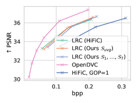
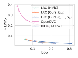
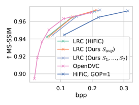
We evaluated the learned models using PSNR, LPIPS and MS-SSIM and compared the latent residual compression (LRC) model to OpenDVC. Figure 9 shows that our LRC models capture details (e.g. textures of the street and trees), while OpenDVC oversmoothes the texture details at the same bitrate. To obtain the rate distortion curve (Figure 10) we trained a video compression model for each of $\text{\emph{HiFiC}}^{\{Hi,Mi,Lo\}}$. It can be seen that the LRC model leverages the motion information of previous frames. When compared to $\text{\emph{HiFiC}}^{Lo}$, the LRC model decreases the bitrate by almost 50% (0.056bpp vs 0.11bpp) while keeping the reconstruction quality at a similar level. In case of $\text{\emph{HiFiC}}^{Hi}$, the improvement in terms of percentage is less, namely (~$30$%). The results also show that using the distilled decoder LRC (Ours $\mathcal{S}_{uvg}$) produces similar quality of reconstruction and only adds 0.005bpp if encoded on the full UVG dataset (3900 frames). The content-specific information that has to be additionally sent is already included in the numbers and amortized over the full dataset. Such information is sent uncompressed. Also, it can be seen that if we overfit to each sequence separately the model can better adapt to each sequence with the trade-off of sending the weights for each subset. This explains the increase of bpps for LRC (Ours $\mathcal{S}_{1},\dots,\mathcal{S}_{7}$).

(a)

(b)

(c)

Figure 10: Results for neural video codecs on UVG Dataset. The points on the curve correspond to (left) $\text{\emph{HiFiC}}^{Lo}$, (mid) $\text{\emph{HiFiC}}^{Mi}$ and (right) $\text{\emph{HiFiC}}^{Hi}$. If not noted, GOP=10. The content-specific information per subset is included in the plots and amortized over the full dataset.

5 Conclusion

In this paper, we showed how to leverage knowledge distillation in the context of neural image and video compression. More specifically we focused on GAN-based neural networks targeting low bitrates. Our proposal distills the information from a big decoder and replaces it with a much smaller one along with sequence-specific side information. Altogether this allows us to have only ~5% of the original model size and to achieve 50% reduction in decoding time. Future work could focus on appropriate encoding of the side information and additional methods to ensure temporal consistency.

Appendix A Appendix

A.1 Knowledge Distillation for Video Compression with Latent Space Residuals

Let consider the sequence of frames $\mathbf{x}_{0},\dots,\mathbf{x}_{GOP}$. To compress the full sequence, the I-Frame or Keyframe ($\mathbf{x}_{0}$) is compressed by an image compression codec to $\hat{\mathbf{x}}_{0}$. Given this compressed I-Frame, the codec computes the flow field $\mathbf{f}=\left(\mathbf{f}_{y},\mathbf{f}_{x}\right)$ to the next frame. The decompressed flow field $\hat{\mathbf{f}}$ is then used to warp the previous frame $\hat{\mathbf{x}}^{warp}_{t+1}=\operatorname{billinear}\left(\hat{\mathbf{x}}_{t},\hat{\mathbf{f}}\right)$. Similar as in [Lu et al., 2019a] we use a Motion Compensation network to fix obvious errors of the warp, which eventually results in the final prediction $\mathbf{x}_{t+1}^{Pred}$. To compress the optical flow $\mathbf{f}$ we use the same auto encoder architecture as proposed in [Ballé et al., 2018]. In our implementation we use spatial pyramid network [Ranjan and Black, 2016] for flow field estimation.

To compute the latent residuals, we first encode both frames, $\mathbf{x}_{t+1}^{Pred}$ and $\mathbf{x}_{t+1}$ with the pre-trained HiFiC encoder and take the difference of the encodings $\mathbf{r}_{t+1}=\mathbf{y}_{t+1}-\mathbf{y}^{Pred}_{t+1}$. The probability distribution of the residuals is then learned with a Scale-Hyperprior [Ballé et al., 2018]. By adding the decompressed residuals and the encodings of the prediction $\hat{\mathbf{y}}_{t+1}=\hat{\mathbf{r}}_{t+1}+\mathbf{y}^{Pred}_{t+1}$ we obtain the latents of the next frame $\hat{\mathbf{x}}_{t+1}$.

The training of the model is separated into four stages. In the first stage, we only train the motion vector compression network. The loss we optimize is defined as:

$$\mathcal{L}_{warp}=\lambda_{w}r\left(\hat{\mathbf{w}}_{t+1}\right)+\operatorname{MSE}\left(\mathbf{x}_{t+1},\hat{\mathbf{x}}^{warp}_{t+1}\right)$$ (2)

where $\mathbf{w}_{t+1}$ is the encoding of flow field $\mathbf{f}$ and $\lambda_{w}$ is a hyperparameter controlling the trade-off between the distortion term and the rate term $r\left(\hat{\mathbf{w}}_{t+1}\right)$.

In the second phase, the Motion Compensation network is trained by optimizing the following loss:

$$\mathcal{L}_{mc}=\lambda_{w}r\left(\hat{\mathbf{w}}_{t+1}\right)+k_{M}\operatorname{MSE}\left(\mathbf{x}_{t+1},\mathbf{x}_{t+1}^{Pred}\right)+k_{M}L_{1}\left(\mathbf{y}_{t+1},\mathbf{y}^{Pred}_{t+1}\right).$$ (3)

Note, that the $L_{1}$ forces the model to learn predictions with latents close to latents of the ground truth image $\mathbf{x}_{t+1}$.

The loss of the third phase is defined as:

$$\mathcal{L}_{step}=\lambda_{w}\left(r\left(\hat{\mathbf{w}}_{t+1}\right)+r\left(\hat{\mathbf{r}}_{t+1}\right)\right)+k_{M}\operatorname{MSE}\left(\tilde{\mathbf{x}}_{t+1},\hat{\mathbf{x}}_{t+1}\right)+k_{p}d_{p}\left(\mathbf{x}_{t+1},\hat{\mathbf{x}}_{t+1}\right).$$ (4)

Important to note, in this phase we make use of the teacher-decoder. We minimize the loss between the compressed P-Frame $\hat{\mathbf{x}}_{t+1}$ and the HiFiC compressed frame $\tilde{\mathbf{x}}_{t+1}$.

In the fourth and final phase we optimize for $N=3$ frames in one optimization step, to consider more temporal information and alleviate error accumulation Lu et al. [2020]:

$$\mathcal{L}_{final}=\lambda\sum^{N}_{i=1}\left(r\left(\hat{\mathbf{w}}_{i}\right)+r\left(\hat{\mathbf{r}}_{i}\right)\right)+\sum^{N}_{i=1}k_{M}\operatorname{MSE}\left(\tilde{\mathbf{x}}_{i},\hat{\mathbf{x}}_{i}\right)+k_{p}d_{p}\left(\mathbf{x}_{i},\hat{\mathbf{x}}_{i}\right),$$ (5)

References

- Agustsson et al. (2019) Eirikur Agustsson, Michael Tschannen, Fabian Mentzer, Radu Timofte, and Luc Van Gool. Generative adversarial networks for extreme learned image compression. In The IEEE International Conference on Computer Vision (ICCV), October 2019.
- Ballé et al. (2016) Johannes Ballé, Valero Laparra, and Eero P. Simoncelli. End-to-end optimized image compression. CoRR, abs/1611.01704, 2016. URL http://arxiv.org/abs/1611.01704.
- Ballé et al. (2017) Johannes Ballé, Valero Laparra, and Eero P Simoncelli. End-to-end optimized image compression. ICLR, 2017.
- Ballé et al. (2018) Johannes Ballé, David Minnen, Saurabh Singh, Sung Jin Hwang, and Nick Johnston. Variational image compression with a scale hyperprior. ICLR, 2018.
- Beyer et al. (2021) Lucas Beyer, Xiaohua Zhai, Amélie Royer, Larisa Markeeva, Rohan Anil, and Alexander Kolesnikov. Knowledge distillation: A good teacher is patient and consistent. arXiv preprint arXiv:2106.05237, 2021.
- Brock et al. (2018) Andrew Brock, Jeff Donahue, and Karen Simonyan. Large scale GAN training for high fidelity natural image synthesis. CoRR, abs/1809.11096, 2018. URL http://arxiv.org/abs/1809.11096.
- Chang and Lu (2020) Ting-Yun Chang and Chi-Jen Lu. Tinygan: Distilling biggan for conditional image generation. CoRR, abs/2009.13829, 2020. URL https://arxiv.org/abs/2009.13829.
- Choi et al. (2019) Yoojin Choi, Mostafa El-Khamy, and Jungwon Lee. Variable rate deep image compression with a conditional autoencoder. In 2019 IEEE/CVF International Conference on Computer Vision, ICCV 2019, Seoul, Korea (South), October 27 - November 2, 2019, pages 3146–3154. IEEE, 2019. doi: 10.1109/ICCV.2019.00324. URL https://doi.org/10.1109/ICCV.2019.00324.
- Djelouah et al. (2019a) Abdelaziz Djelouah, Joaquim Campos, Simone Schaub-Meyer, and Christopher Schroers. Neural inter-frame compression for video coding. In 2019 IEEE/CVF International Conference on Computer Vision, ICCV 2019, Seoul, Korea (South), October 27 - November 2, 2019, pages 6420–6428. IEEE, 2019a. doi: 10.1109/ICCV.2019.00652. URL https://doi.org/10.1109/ICCV.2019.00652.
- Djelouah et al. (2019b) Abdelaziz Djelouah, Joaquim Campos, Simone Schaub-Meyer, and Christopher Schroers. Neural inter-frame compression for video coding. In Proceedings of the IEEE International Conference on Computer Vision, pages 6421–6429, 2019b.
- Fab (2015) BPG Specification. Fabrice Bellard, 2015. version 0.9.5.
- Helminger et al. (2020) Leonhard Helminger, Abdelaziz Djelouah, Markus Gross, and Christopher Schroers. Lossy image compression with normalizing flows. arXiv preprint arXiv:2008.10486, 2020.
- Hepburn et al. (2021) Alexander Hepburn, Valero Laparra, Raúl Santos-Rodríguez, Johannes Ballé, and Jesús Malo. On the relation between statistical learning and perceptual distances. CoRR, abs/2106.04427, 2021. URL https://arxiv.org/abs/2106.04427.
- Kingma and Ba (2015) Diederik P. Kingma and Jimmy Ba. Adam: A method for stochastic optimization. In Yoshua Bengio and Yann LeCun, editors, 3rd International Conference on Learning Representations, ICLR 2015, San Diego, CA, USA, May 7-9, 2015, Conference Track Proceedings, 2015. URL http://arxiv.org/abs/1412.6980.
- Ladune et al. (2021) Théo Ladune, Pierrick Philippe, Wassim Hamidouche, Lu Zhang, and Olivier Déforges. Conditional coding for flexible learned video compression. arXiv preprint arXiv:2104.07930, 2021.
- Lu et al. (2019a) Guo Lu, Wanli Ouyang, Dong Xu, Xiaoyun Zhang, Chunlei Cai, and Zhiyong Gao. DVC: an end-to-end deep video compression framework. In IEEE Conference on Computer Vision and Pattern Recognition, CVPR 2019, Long Beach, CA, USA, June 16-20, 2019, pages 11006–11015. Computer Vision Foundation / IEEE, 2019a. doi: 10.1109/CVPR.2019.01126. URL http://openaccess.thecvf.com/content_CVPR_2019/html/Lu_DVC_An_End-To-End_Deep_Video_Compression_Framework_CVPR_2019_paper.html.
- Lu et al. (2019b) Guo Lu, Wanli Ouyang, Dong Xu, Xiaoyun Zhang, Chunlei Cai, and Zhiyong Gao. Dvc: An end-to-end deep video compression framework. In CVPR, 2019b.
- Lu et al. (2020) Guo Lu, Chunlei Cai, Xiaoyun Zhang, Li Chen, Wanli Ouyang, Dong Xu, and Zhiyong Gao. Content adaptive and error propagation aware deep video compression. In Andrea Vedaldi, Horst Bischof, Thomas Brox, and Jan-Michael Frahm, editors, Computer Vision - ECCV 2020 - 16th European Conference, Glasgow, UK, August 23-28, 2020, Proceedings, Part II, volume 12347 of Lecture Notes in Computer Science, pages 456–472. Springer, 2020. doi: 10.1007/978-3-030-58536-5\_27. URL https://doi.org/10.1007/978-3-030-58536-5_27.
- Mentzer et al. (2018) Fabian Mentzer, Eirikur Agustsson, Michael Tschannen, Radu Timofte, and Luc Van Gool. Conditional probability models for deep image compression. In CVPR, 2018.
- Mentzer et al. (2020) Fabian Mentzer, George Toderici, Michael Tschannen, and Eirikur Agustsson. High-fidelity generative image compression. CoRR, abs/2006.09965, 2020. URL https://arxiv.org/abs/2006.09965.
- Mercat et al. (2020) Alexandre Mercat, Marko Viitanen, and Jarno Vanne. Uvg dataset: 50/120fps 4k sequences for video codec analysis and development. In Proceedings of the 11th ACM Multimedia Systems Conference, MMSys ’20, page 297–302, New York, NY, USA, 2020. Association for Computing Machinery. ISBN 9781450368452. doi: 10.1145/3339825.3394937. URL https://doi.org/10.1145/3339825.3394937.
- Minnen et al. (2018) David Minnen, Johannes Ballé, and George D Toderici. Joint autoregressive and hierarchical priors for learned image compression. In NeurIPS. 2018.
- NYTimes (2020) NYTimes. The virus changed the way we internet. https://www.nytimes.com/interactive/2020/04/07/technology/coronavirus-internet-use.html, 2020. Accessed: 2021-10-20.
- Patel et al. (2019a) Yash Patel, Srikar Appalaraju, and R. Manmatha. Deep perceptual compression. CoRR, abs/1907.08310, 2019a. URL http://arxiv.org/abs/1907.08310.
- Patel et al. (2019b) Yash Patel, Srikar Appalaraju, and R. Manmatha. Human perceptual evaluations for image compression. CoRR, abs/1908.04187, 2019b. URL http://arxiv.org/abs/1908.04187.
- Patel et al. (2021) Yash Patel, Srikar Appalaraju, and R. Manmatha. Saliency driven perceptual image compression. In Proceedings of the IEEE/CVF Winter Conference on Applications of Computer Vision (WACV), pages 227–236, January 2021.
- Ranjan and Black (2016) Anurag Ranjan and Michael J. Black. Optical flow estimation using a spatial pyramid network. CoRR, abs/1611.00850, 2016. URL http://arxiv.org/abs/1611.00850.
- Toderici et al. (2016) George Toderici, Sean M O’Malley, Sung Jin Hwang, Damien Vincent, David Minnen, Shumeet Baluja, Michele Covell, and Rahul Sukthankar. Variable rate image compression with recurrent neural networks. ICLR, 2016.
- Toderici et al. (2017) George Toderici, Damien Vincent, Nick Johnston, Sung Jin Hwang, David Minnen, Joel Shor, and Michele Covell. Full resolution image compression with recurrent neural networks. In CVPR, 2017.
- van Rozendaal et al. (2021) Ties van Rozendaal, Iris AM Huijben, and Taco S Cohen. Overfitting for fun and profit: Instance-adaptive data compression. arXiv preprint arXiv:2101.08687, 2021.
- Veerabadran et al. (2020) Vijay Veerabadran, Reza Pourreza, AmirHossein Habibian, and Taco Cohen. Adversarial distortion for learned video compression. In 2020 IEEE/CVF Conference on Computer Vision and Pattern Recognition, CVPR Workshops 2020, Seattle, WA, USA, June 14-19, 2020, pages 640–644. IEEE, 2020. doi: 10.1109/CVPRW50498.2020.00092. URL https://doi.org/10.1109/CVPRW50498.2020.00092.
- Wang et al. (2021) Longguang Wang, Yingqian Wang, Xiaoyu Dong, Qingyu Xu, Jungang Yang, Wei An, and Yulan Guo. Unsupervised degradation representation learning for blind super-resolution. CoRR, abs/2104.00416, 2021. URL https://arxiv.org/abs/2104.00416.
- Zhang et al. (2018) Richard Zhang, Phillip Isola, Alexei A Efros, Eli Shechtman, and Oliver Wang. The unreasonable effectiveness of deep features as a perceptual metric. In Proceedings of the IEEE conference on computer vision and pattern recognition, pages 586–595, 2018.