QN Optimization with Hessian Samples

Abstract

This article explores how to effectively incorporate curvature information generated using SIMD-parallel forward-mode Algorithmic Differentiation (AD) into unconstrained Quasi-Newton (QN) minimization of a smooth objective function, $f$. Specifically, forward-mode AD can be used to generate block Hessian samples $Y=\nabla^{2}f(x)\,S$ whenever the gradient is evaluated. Block QN algorithms then update approximate inverse Hessians, $H_{k}\approx\nabla^{2}f(x_{k})$, with these Hessian samples. Whereas standard line-search based BFGS algorithms carefully filter and correct secant-based approximate curvature information to maintain positive definite approximations, our algorithms directly incorporate Hessian samples to update indefinite inverse Hessian approximations without filtering. The sampled directions supplement the standard QN two-dimensional trust-region sub-problem to generate a moderate dimensional subproblem which can exploit negative curvature. The resulting quadratically-constrained quadratic program is solved accurately with a generalized eigenvalue algorithm and the step advanced using standard trust region step acceptance and radius adjustments. The article aims to avoid serial bottlenecks, exploit accurate positive and negative curvature information, and conduct a preliminary evaluation of selection strategies for $S$.

68W20, 68W2, 65F35, 90C53

1 Literature Discussion

Schnable [Sch87] first discusses incorporating parallel function evaluations to improve Hessian approximation in optimization algorithms. Together with his colleagues, Byrd, Schnable, and Shultz [BSS88a, BSS88b] supplement several standard Quasi Newton optimization schemes with a small number of finite difference second derivative approximations and conclude that the supplemental information improves all the variants considered. Their study includes the underlying QN update, the update order within each step, and a variety of strategies to choose a few supplemental directions. In their conclusions Byrd, Schnable, and Shultz [BSS88b] suggest supplementing the extremely simple Symmetric-Rank-One (SR1) QN update with additional second derivative information: the motivation for this suggestion is that Conn, Gould and Toint find in [CGT88] that SR1 is better than Powell-Symmetric-Broyden (PSB), Davidon-Fletcher-Powell (DFP), and Broyden–Fletcher–Goldfarb–Shanno (BFGS). The review article by Schnable [Sch95] summarizes this and other early parallel optimization approaches. More recently, Gau and Goldfarb [GG18] implemented and tested line-search based algorithms using block BFGS updates on subsets of previous directions, and a family of Quasi-Newton algorithm [GG19] which avoids a line-search for a restricted class of cost functions. In yet another approach, Berahasa, Jahanib, Richtarik and Takac [BJRT21] develop zero-memory Block-BFGS and block-SR1 algorithm using only one (the most recent) set of AD generated Hessian samples. Their BFGS variant is implemented with a Line-Search (requiring a positive definite approximate Hessian) while their SR1 variant is implemented with a Conjugate Gradient based approximate solution of a full dimensional trust region sub problem.

The review article [MTK03] and the articles in the associated special edition of Parallel Computing emphasize improving the parallel efficiency of the underlying linear algebra and introducing parallelism through simultaneous (with different starting points and/or different but possibly related QN updates) line searches. The second-order section of the extensive review article [BCN18] provides a more recent update with a focus on algorithms for very high dimensional problems.

A number of recent developments make it appropriate to revisit the topics in [BSS88b] with modern computational tools. The GPU-enabled forward-mode Algorithmic Differentiation (AD), implemented in the open-source computational tool Julia [RLP16] and other software projects, can efficiently replace the finite difference approximations used in [BSS88b] and greatly increases the number of simultaneous Hessian samples. The generalized eigenvalue based trust-region sub-problem solver developed by Adachi et al. [AINT17] can replace the line search with an accurate and robust moderate-dimensional trust-region sub-problem (TRSP), implemented in Julia [RGN21].

The goal of this manuscript is to incorporate SIMD-parallel Hessian samples into QN updates to generate provably convergent QN like algorithms. The proposed algorithms avoid serial bottlenecks by using indefinite approximate Hessians. The standard two-dimensional TRSP minimizes a quadratic model over the span of the steepest-descent and Newton directions. This 2D search space is extended (through a specific Hessian re-sampling strategy) to include additional supplementary directions with accurate curvature information on the resulting moderate dimensional sub-space. With standard trust-region controls this gives a provably convergent algorithm with rapid asymptotic convergence to non-degenerate local minimizers.

The article explores two simple indefinite updates (a block variant of SR1 and a block variant of Powell Symmetric Broyden) which can be directly implemented on accurate AD curvature information. In contrast, line-search based block methods (such as a block BFGS or DFP) need to carefully filter and correct approximate curvature information to maintain positive definite Hessian approximations. The article explores how the selection strategy for and number of supplementary directions affects the algorithms based on these two standard indefinite QN updates.

Section 2 introduces essential assumptions and notation. Section 3 discusses the choices made to evaluate curvature information using Algorithmic Differentiation (AD). Section 4 discusses the advantages of indefinite QN updates for trust-region optimization, explains why block BFGS and DFP are not suitable, and presents the simple and highly-parallel block SR1 and PSB updates used. Section 5 describes the trust-region sub-problem underlying the algorithm. Section 6 explains how new supplemental directions are chosen. Section 7 describes the assembled algorithm including: a simple mean curvature estimate used to initialize $H$; a simple initial trust region radius $\Delta_{0}$ based on the curvature in the steepest descent direction; standard trust region control; cost evaluation; and pseudo code. Section 8 describes our numerical experiments. Section 9 summarizes the results and future plans.

2 Notation and Assumptions

We assume throughout we are seeking the unconstrained minimum of a $C^{2}$ function $f:\mathbb{R}^{n}\rightarrow\mathbb{R}$, with gradient $g(x)=\nabla f(x)$ given by $g:\mathbb{R}^{n}\rightarrow\mathbb{R}^{n}$, and that we can efficiently sample the Jacobian of $g$ (which is the Hessian of $f$) $J(x)=\nabla g(x)=\nabla^{2}f(x)$ using forward-mode AD. In this context, sample the Hessian means that whenever we compute $g(x)=\nabla f(x)$ we can efficiently and simultaneously compute $Y=J(x)\,S\in\mathbb{R}^{n\times w}$ for a block of $w$ directions, $S\in\mathbb{R}^{n\times w}$. We write orth($M$) for an orthogonalization of $M$ (implemented as Matrix(qr(M).Q) in Julia), $M^{\dagger}_{\delta}$ (implemented as pinv($M$; rtol = $\delta$) in Julia) for the $\delta$ thresholded pseudo-inverse of $M$, and $M\sim\mathcal{N}_{0,1}^{n\times w}$ (implemented as randn(n,w)) for an $n\times w$ matrix with elements drawn from the standard normal distribution. We denote the current search point by $x_{k}$ with: objective function value $f_{k}=f(x_{k})$; gradient $g_{k}=g(x_{k})=\nabla f(x_{k})$; Jacobian $J_{k}=J(x_{k})=\nabla^{2}f(x_{k})$; and $h_{k}=h(x_{k})$ where $h(x)=J(x)\,g(x)=\nabla^{2}f(x)\nabla f(x)$. Symmetric Quasi-Newton (QN) approximations $B_{k}$ and $H_{k}$ are updated (using indefinite updates which can incorporate negative curvature information) to satisfy $B_{k}\approx J_{k}$ and $H_{k}\approx J_{k}^{-1}$. The Frobenius inner product of matrices $A$ and $B$ is denoted by $\left<A,B\right>_{F}$ and the Frobenius norm $||A||_{F}^{2}=\left<A,A\right>_{F}$ is used throughout.

3 Algorithmic Differentiation and Hessian Samples

In our context, sampling the Hessian means that whenever we compute $g(x)=\nabla f(x)$, we can efficiently and simultaneously compute $Y=\nabla^{2}f(x)\,S\in\mathbb{R}^{n\times w}$ for a block of $w$ directions $S\in\mathbb{R}^{n\times w}$. The Julia ForwardDiff package [RLP16] modifies the code of $g$ to code $\mbox{\tt gAD}(x,S):\mathbb{R}^{n}\times\mathbb{R}^{n\times w}\rightarrow\mathbb{R}^{n}\times\mathbb{R}^{n\times w}$ for the simultaneous combined computation. In practice, gAD is embarrassingly SIMD parallel. Provided $w$ does not exceed the available processor resources, evaluating $\mbox{\tt gAD}(x,S)$ takes only $2-3$ times as long as evaluating $g(x)$. Since modern GPUs have over $256$ cores organized into SIMD warps of 8, 16 or 32 threads, values of $w\leq 256$ are feasible on most commodity modern hardware with much larger values feasible on specialized hardware.

The algorithm we will generate centers around generating accurate curvature information at a single point for the steepest descent direction, in addition to other sampled directions. To accomplish this, the curvature information Incorporated in Algorithm 1 is generated by two sequential gAD calls. A first call to gAD computes the gradient and a first Hessian sample $(g,Y_{1})\leftarrow\mbox{\tt gAD}(x,S_{1})$. The gradient, $g$, is included in a second direction set $S_{2}$ so that the Hessian sample $Y_{2}$ computed by $\mbox{\tt gAD}(x,S_{2})$ contains $h(x)=J(x)\,g(x)=\nabla^{2}f(x)\,\nabla f(x)$. This can be organized in a number of ways. Algorithm 1 gives the simple (and almost certainly non-optimal) choices made for a combined gradient and Hessian Sample operation $\mbox{\tt gHS}(x,S)$.

Algorithm 1 Gradient and Hessian Sample: $(g,h,Y)\leftarrow\mbox{\tt gHS}(x,S)$

0:   $x\in\mathbb{R}^{n}$ and $S\in\mathbb{R}^{n\times(2w-1)}$.

1:  Compute $\left(g,Y_{1}\right)\leftarrow\mbox{\tt gAD}(x,S\left[\;:\;,\;1:w\;\right])$ {Input the first $w$ columns of $S$ to gAD}

2:  Compute $\displaystyle\left(g,Y_{2}\right)\leftarrow\mbox{\tt gAD}\left(x,\left[\;S\left[\;:\;,\;w+1\!:\!\text{end}\;\right]\,,\,g\;\right]\right)$ {Input the last $w-1$ columns of $S$ and $g$ to gAD}

3:  Assemble $Y\leftarrow[\;Y_{1}\;,\;Y_{2}[\;:\;,\;1:\text{end}-1]\;]$

4:  return  $\left(g,Y_{2}[\;:\;,\;\text{end}\;],\;Y\right)$ {By construction, $Y_{2}[\;:\;,\;\text{end}\;]=\nabla^{2}f(x)\,g$}

4 Quasi-Newton Updates

Several Quasi-Newton updates (with a variety of update details) are tested in [BSS88a]. The subsequent article [BSS88b] which focuses on the now dominant BFGS algorithm notes that an indefinite SR1 update might work well, as evidenced in an almost contemporaneous article [CGT88]. In this preliminary study we use the indefinite block SR1 and PSB algorithms to incorporate a block of accurate Hessian samples $Y=\nabla^{2}f(x_{k+1})\,S$ after successful steps. We explore the effect of including a standard secant curvature estimates $\left(\nabla f(x_{k+1})-\nabla f(x_{k})\right)\approx\nabla f^{2}(x_{k})\left(x_{k+1}-x_{k}\right)$ before the block update and including the prior step in the block update. The Hessian is not updated on a failed step since the gradient is not evaluated and there is no new curvature information.

Conn, Gould and Toint [CGT88] present evidence that when the underlying Hessian is indefinite, SR1 (with suitable globalization strategies for indefinite Hessian approximations) can outperform updates (like BFGS) designed to maintain positive definite Hessian approximations. We use a globalization strategy (the moderate dimensional trust region presented in Section 5) which can exploit negative curvature and select QN updates suitable for indefinite approximations.

Block versions of updates which implicitly use the current Hessian (such as BFGS and DFP) require care when the Hessian is indefinite. We explain the issues for the block BFGS update in Algorithm 2 [BSS88b, BSS88a] which incorporates a block of curvature estimates $\widehat{V}\approx\nabla^{2}f(x)\,U$ into an inverse Hessian approximation $H^{-1}\approx\nabla^{2}f(x)$.

Algorithm 2 block BFGS Update: $H_{\text{BFGS}}\leftarrow{\tt BFGS}(H,U,\widehat{V},\delta)$.

0:   SPD $H\in\mathbb{R}^{n\times n}$ and $U,\widehat{V}\in\mathbb{R}^{n\times 2w}$ with $U^{\top}\widehat{V}$ approximately symmetric

1:   Filter and correct $\widehat{V}$ to $V$ consistent with $V=A\,U$ for some SPD $A$.

2:  Compute $T\leftarrow\left(U^{\top}V\right)^{\dagger}_{\delta}$.

3:  return  $U\,T\,U^{\top}+\left(I-U\,T\,V^{\top}\right)H\left(I-V\,T\,U^{\top}\right)$.

There are two reasons for the initial filtering step in line of Algorithm 2. Finite difference approximations and/or multiple secant estimates generate approximations $\widehat{V}\approx\nabla^{2}f(x)\,U$, however, $\widehat{V}$ needs to be corrected to ensure $U^{\top}\widehat{V}$ is symmetric. When $\nabla^{2}f(x)$ is not positive definite, negative curvature directions in $\widehat{V}\approx\nabla^{2}f(x)\,U$ need to be filtered to ensure $H_{\text{BFGS}}$ is SPD. These corrections and filters [BSS88b, BSS88a, BJRT21] are inherently serial. In contrast, there is no need to correct accurate AD Hessian samples $V=\nabla^{2}f(x)\,U=J(x)\,U$ from $\mbox{\tt gHS}(x,S)$ or filter negative curvature directions for trust region based algorithms which can use indefinite Hessian approximations $H$. Note the BFGS update is a critical point of

(1) $$\operatorname*{arg\,min}_{A\,V=U,A=A^{\top}}\left<\;(H-A)\,\mathcal{J}^{-1}\;,\;(H-A)\;\right>_{F}$$

for any invertible $\mathcal{J}$ consistent with the sample in the sense that $U^{\top}V=U^{\top}\mathcal{J}\,U$. Running BFGS without filtering produces meaningless updates since if $U^{\top}V$ is not SPD Eq. 1 gives a saddle point of an unbounded minimization problem.

We test two indefinite block QN updates with identical trust-region sub-solvers and controls. Algorithm 3 specifies block Symmetric Rank 1 (block SR1) which is a direct block generalization [BJRT21] of the rank one SR1 update: block SR1 is the algebraically minimal update $H_{\text{SR1}}$ which satisfies the block inverse secant condition $H_{\text{SR1}}V=U$. Algorithm 4 specifies block Powell-Symmetric-Broyden (block PSB) which is a direct block generalization of the rank two Powell-Symmetric-Broyden (PSB) update [BSS88a, BSS88b]: block PSB is the minimal Frobenius norm change satisfying the block inverse secant condition $H_{\text{PSB}}V=U$, i.e.,

$$H_{\text{PSB}}=\operatorname*{arg\,min}_{AV=U,A=A^{\top}}||H-A||_{F}=\operatorname*{arg\,min}_{AV=U,A=A^{\top}}\left<\;H-A\;,\;H-A\;\right>_{F}.$$

0:   $H\in\mathbb{R}^{n\times n}$ with $H=H^{\top}$; $U,V\in\mathbb{R}^{n\times 2w}$ with $U^{\top}V=V^{\top}U$; $\delta>0$.

1:  Compute $T\leftarrow((U-H\,V)^{\top}V)^{\dagger}_{\delta}$.

2:  return  $H+\left(U-H\,V\right)T\left(U-H\,V\right)^{\top}$.

Algorithm 3 block SR1 Update: $H_{\text{SR1}}\leftarrow$ SR1$(H,U,V,\delta)$.

Algorithm 4 block PSB Update: $H_{\text{PSB}}\leftarrow{\tt PSB}(H,U,V,\delta)$.

0:   $H\in\mathbb{R}^{n\times n}$ with $H=H^{\top}$; $U,V\in\mathbb{R}^{n\times 2w}$ with $U^{\top}V=V^{\top}U$; $\delta>0$.

1:  Compute $T_{1}\leftarrow\left(V^{\top}V\right)^{\dagger}_{\delta}$.

2:  Compute $T_{2}\leftarrow VT_{1}(U-HV)^{\top}$.

3:  return  $H+T_{2}+T_{2}^{\top}-T_{2}\,V\,T_{1}\,V^{\top}$.

Algorithms 3 and 4 do not need to filter accurate curvature information from gHS. The pseudo-inverse tolerance $\delta=10^{-12}$ simply restricts excessively large updates.

Byrd and Schnabel [BSS88b, BSS88a] considered various additional updates and discovered that including the approximate secant curvature information

(2) $$y_{k+1}=(\nabla f_{k+1}-\nabla f_{k})\approx\nabla^{2}f(x_{k+1})p_{k}=\nabla^{2}f(x_{k+1})(x_{k+1}-x_{k})$$

improved their algorithms. They recommend a preliminary QN update with the approximate curvature information Eq. 2 before a second update to incorporate the additional curvature information. We perform numerical experiments which replicate this observation and evaluate a possible block replacement.

5 Trust Region Sub-Problem

Trust region algorithms are based on approximate solutions of the $n$ dimensional quadratically constrained quadratic program

(3) $$p_{k}=\operatorname*{arg\,min}_{|p|\leq\Delta_{k}}\frac{1}{2}p^{\top}H_{k}^{-1}\,p+\nabla f_{k}^{\top}p\quad\mbox{where}\quad H_{k}^{-1}\approx\nabla^{2}f(x_{k}).$$

If $H_{k}$ is full rank Eq. 3 is equivalent (with $p_{k}=H_{k}q_{k}$) to

(4) $$q_{k}=\operatorname*{arg\,min}_{|H_{k}q|\leq\Delta_{k}}m_{k}(q)\quad\mbox{where}\quad m_{k}(q)=\frac{1}{2}q^{\top}H_{k}\,q+(H_{k}\nabla f_{k})^{\top}q.$$

The standard two-dimensional subspace approximation (discussed on p76 of [NW06]) minimizes Eq. 3 for $p=a_{1}\nabla f_{k}+a_{2}H_{k}\nabla f_{k}$.

The sampling procedure $\mbox{\tt gHS}(x_{k},S_{k})$ generates accurate curvature information $[\;Y_{k}\;,\;h_{k}\;]=\nabla^{2}f(x_{k})\,[\;S_{k}\;,\;\nabla f_{k}\;]$ in the directions specified by the columns of $S_{k}$ and $\nabla f_{k}$ and the inverse Hessian approximation, $H_{k}$, is immediately updated (using either Algorithm 2 or Algorithm 3) to match with

$$U=\left[\;S_{k}\;,\;\frac{\nabla f_{k}}{\|\nabla f_{k}\|}\;\right]\quad\mbox{and}\quad V=\left[\;Y_{k}\;,\;\frac{h_{k}}{\|\nabla f_{k}\|}\;\right]$$

The scaling weights all the columns of $V$ equally and maintains a well-conditioned computation when $\nabla f_{k}$ is large or small. Thus,

(5) $$Y_{k}=H_{k}^{-1}S_{k}\quad\mbox{and}\quad h_{k}=H_{k}^{-1}\nabla f_{k}.$$

The standard 2D approximation ($p$ in the span of $\nabla f_{k}$ and $H_{k}\nabla f_{k}$) is expanded with the columns of $S_{k}$ to give the explicit representation $p=M_{k}\,a$ where

$$M_{k}=\left[\;\frac{\nabla f_{k}}{\|\nabla f_{k}\|}\;,\;\frac{H_{k}\nabla f_{k}}{\|\nabla f_{k}\|}\;,\;S_{k}\;\right]\in\mathbb{R}^{n\times(2w+1)},\quad a\in\mathbb{R}^{2w+1}.$$

In terms of $q=H_{k}^{-1}p$, the equivalent representation (since $H_{k}$ is exact on the sample Eq. 5) is $H_{k}^{-1}M_{k}$. We use the orthogonal representation $Q_{k}=\mbox{\tt orth}\left(H_{k}^{-1}M_{k}\right)$ where

(6) $$H_{k}^{-1}M_{k} =\left[\;H_{k}^{-1}\frac{\nabla f_{k}}{\|\nabla f_{k}\|}\;,\;\frac{\nabla f_{k}}{\|\nabla f_{k}\|}\;,\;H_{k}^{-1}S_{k}\;\right]=\left[\;\frac{h_{k}}{\|\nabla f_{k}\|}\;,\;\frac{\nabla f_{k}}{\|\nabla f_{k}\|}\;,\;Y_{k}\;\right].$$

Thus, our new trust-region approximation (with $Q_{k}$ from Eq. 6 and $m_{k}$ from Eq. 4) is

(7) $$a_{k}=\operatorname*{arg\,min}_{a\in\mathbb{R}^{2w+1}:|H_{k}Q_{k}\,a|\leq\Delta_{k}}m_{k}(Q_{k}\,a)$$

giving the trial step $x_{k+1}=x_{k}+p_{k}=x_{k}+H_{k}\,Q_{k}\,a_{k}$. The Julia trs package [NJN21] (developed for [RGN21] based on [AINT17]) computes accurate eigen-value based solutions of

$$a_{k}=\operatorname*{arg\,min}_{a^{\top}Ca\;\leq\;\Delta_{k}^{2}}\frac{1}{2}a^{\top}Pa+b^{\top}a.$$

We use the robust small-scale solver (based on a dense generalized eigenvalue decomposition) and compute accurate solutions of Eq. 7 with

(8) $$a_{k}=\mbox{{\tt trs\_small}}(P,b,\Delta_{k},C)$$

where the arguments are

$$P=Q_{k}^{\top}\,H_{k}\,Q_{k},\quad b=Q_{k}^{\top}\,H_{k}\,\nabla f_{k},\quad\mbox{and}\quad C=Q_{k}^{\top}\,H_{k}^{2}\,Q_{k}.$$

6 Supplemental Directions

Lastly, we need to address how to select the supplementary directions, $S\in\mathbb{R}^{n\times(2w-1)}$, in Algorithm 1. The six supplemental direction variants considered are:

(9a) $$S_{k+1} ={\tt orth}\left(M\right),\mbox{ where }M\sim\mathcal{N}_{0,1}^{n\times(2w-1)};$$

(9b) $$S_{k+1} ={\tt orth}\left(M-S_{k}(S_{k}^{\top}M)\right),\mbox{ where }M\sim\mathcal{N}_{0,1}^{n\times(2w-1)};$$

(9c) $$S_{k+1} ={\tt orth}\left(Y_{k}-S_{k}(S_{k}^{\top}Y_{k})\right);$$

(9d) $$S_{k+1} ={\tt orth}\left(\left[\;{\tt orth}\left(M\right)\;,\;p_{k}\;\right]\right),\mbox{ where }M\sim\mathcal{N}_{0,1}^{n\times(2w-2)};$$

(9e) $$S_{k+1} ={\tt orth}\left(\left[\;{\tt orth}\left(M-S_{k}(S_{k}^{\top}M)\right)\;,\;p_{k}\;\right]\right),\mbox{ where }M\sim\mathcal{N}_{0,1}^{n\times(2w-2)};$$

(9f) $$S_{k+1} ={\tt orth}\left(\left[\;{\tt orth}\left(Y_{k}[\;:\;,\;1:\text{end}\!-\!1]-S_{k}(S_{k}^{\top}Y_{k}[\;:\;,\;1:\text{end}\!-\!1])\right)\;,\;p_{k}\;\right]\right).$$

The idea behind Eq. 9b was to prevent immediate re-sampling (which will happen in the simple randomization Eq. 9a) by orthogonalizing against the immediate previous directions. The idea behind Eq. 9c was to guide the algorithm to accurately resolve eigen-space associated with the larger Hessian eigenvalues. As noted in Section 4, Byrd and Schnabel [BSS88b, BSS88a] perform a preliminary secant update to incorporate the approximate secant curvature information along the previous step $p_{k}=x_{k+1}-x_{k}$ from Eq. 2. A simple block alternative is to include in the $p_{k}$ in $S_{k+1}$ which ensures that the accurate curvature $\nabla^{2}f(x_{k+1})\,p_{k}$ is incorporated in the inverse Hessian. Equations 9d, 9e, and 9f are simply variants of Eqs. 9a, 9b, and 9c which include $p_{k}$.

7 Algorithmic Overview, Motivation, and Details

The primary goals when designing the algorithm was to extract maximal benefit from AD generated curvature information while avoiding linear solves in the potentially large ambient dimension $n$. Secondary goals (which drove many of the details) were a clean flow of information and provably better objective function reduction (at each step) than familiar convergent benchmarks. Algorithm 5 has pseudo code for the assembled algorithm. Some comments are in order.

Line 6: QN algorithms are commonly initialized with a multiple of the identity. The mean of the eigenvalues of $S_{0}^{\top}\nabla f^{2}(x_{0})\,S_{0}=S_{0}^{\top}Y_{0}$ where $Y_{0}=\mbox{\tt gHS}(x_{0},S_{0})$ provides a natural estimate for this multiplier. This initialization is immediately updated with the QN update to give $H_{0}$ satisfying $Y_{0}=H_{0}S_{0}$.

Lines 5, 12 & 13: We adopt the simple standard strategy and terminology from [NW06] for updating the radius $\Delta_{k}$ and accepting or rejecting the trial step $x_{k}+H_{k}\,Q_{k}\,a_{k}$. Model quality is assessed by measuring the ratio of the actual decrease of the objective function, ${f_{k}-f(x_{k}+H_{k}\,Q_{k}\,a_{k})}$, to the model decrease, $m_{k}(0)-m_{k}(Q_{k}\,a_{k})$, viz.,

(10) $$\rho=\frac{f_{k}-f(x_{k}+H_{k}\,Q_{k}\,a_{k})}{m_{k}(0)-m_{k}(Q_{k}\,a_{k})}.$$

The trust-region radius is updated (our experiments use the large maximum trust region radius $\Delta_{\mbox{max}}=100$) as follows

(11) $$\Delta_{k+1}=\left\{\begin{array}[]{rl}0.25\Delta_{k}&\mbox{if }\rho<0.25\\ \min\left(2\Delta_{k},\Delta_{\mbox{max}}\right)&\mbox{if }\rho>0.75\mbox{ and }||H_{k}Q_{k}a_{k}||=\Delta_{k}\\ \Delta_{k}&\mbox{otherwise}\end{array}\right..$$

We reject the step if $\rho\leq 0$ (this is the standard [NW06] trust-region control with rejection parameter $\eta=0$): we retain all previous values with the updated subscript $k+1$ except the radius $\Delta_{k}$ and recompute Eq. 8 with the $\Delta_{k+1}=0.25\Delta_{k}$ since $\rho<0.25$. We accept the step if $\rho>0$. We set $x_{k+1}=x_{k}+H_{k}Q_{k}a_{k}$ and $f_{k+1}=f(x_{k+1})$ then resample Hessians and update QN approximations. The initial trust-region radius is set to $1.1\times$ the distance to the isotropic quadratic critical point with mean curvature $\alpha_{0}$. In our experiments $\Delta_{\tt max}=100$.

Algorithm 5 Trust Region Quasi-Newton Optimization with Hessian Samples

0:   Convergence tolerance $\epsilon>0$; Pseudo-Inverse tolerance $\delta>0$; Initial point $x_{0}\in\mathbb{R}^{n}$; function handle $f$; Preliminary QN update flag, pflag.

1:  Compute $f_{0}\leftarrow f(x_{0})$; Draw $M\sim\mathcal{N}_{0,1}^{n\times(2w-1)}$; Set $S_{0}\leftarrow{\tt orth}\left(M\right)$.

2:  Compute $\left(\nabla f_{0},h_{0},Y_{0}\right)\leftarrow\mbox{\tt gHS}(x_{0},S_{0})$. {see Algorithm 1}

3:  Construct $\displaystyle U_{0}=\left[\;S_{0}\;,\;\frac{\nabla f_{0}}{\|\nabla f_{0}\|}\;\right]$ and $\displaystyle V_{0}=\left[\;Y_{0}\;,\;\frac{h_{0}}{\|\nabla f_{0}\|}\;\right]$.

4:  Compute initial mean curvature estimate $\alpha_{0}={\tt mean}({\tt eig}(S_{0}^{\top}Y_{0}))$.

5:  Compute initial $\Delta_{0}=\min\left(1.1\times\frac{\|\nabla f_{0}\|}{2|\alpha_{0}|}\;,\;\Delta_{\tt max}=100\right)$.

6:  Initialize $H_{0}\leftarrow\mbox{\tt QN}\left(\alpha^{-1}I,U_{0},V_{0},\delta\right)$. {See Algorithms 2 and 3}

7:  Set $\displaystyle Q_{0}=\mbox{\tt orth}\left(\left[\;\frac{h_{0}}{\|\nabla f_{0}\|}\;,\;\frac{\nabla f_{0}}{\|\nabla f_{0}\|}\;,\;Y_{0}\;\right]\right)$. {See Eq. 6}

8:  Compute $P\leftarrow Q_{0}^{\top}\,H_{0}\,Q_{0};\quad b\leftarrow Q_{0}^{\top}\,H_{0}\,\nabla f_{0};\quad C\leftarrow Q_{0}^{\top}\,H_{0}^{2}\,Q_{0}$. {See Eq. 8}

9:  repeat {$k=0,1,\ldots$}

10:     Compute $a_{k}\leftarrow\mbox{{\tt trs\_small}}(P,b,\Delta_{k},C)$. {from Julia TRS package}

11:     Compute $p_{k}\leftarrow H_{k}Q_{k}a_{k}$,  $f_{k+1}\leftarrow f(x_{k}+p_{k})$ and $\rho$ given by Eq. 10.

12:      Update $\Delta_{k+1}$ according to Eq. 11.

13:     if  $\rho\leq 0$ then

14:        Set $x_{k+1}\leftarrow x_{k};\quad f_{k+1}\leftarrow f_{k};\quad\nabla f_{k+1}\leftarrow\nabla f_{k};\quad H_{k+1}\leftarrow H_{k}$. {Reject Step}

15:     else

16:        Set $x_{k+1}\leftarrow x_{k}+p_{k}$. {Accept Step}

17:        Pick new supplemental directions, $S_{k+1}$, using one of Eqs. 9a, 9b, 9c, 9d, 9e, and 9f .

18:        Compute $\left(\nabla f_{k+1},h_{k+1},Y_{k+1}\right)\leftarrow\mbox{\tt gHS}(x_{k+1},S_{k+1})$.

19:        if pflag then

20:            $H_{k}\leftarrow\mbox{\tt QN}(H_{k},p_{k},\nabla f_{k+1}-\nabla f_{k},\delta)$

21:        end if

22:        Construct $\displaystyle U_{k+1}=\left[\;S_{k+1}\;,\;\frac{\nabla f_{k+1}}{\|\nabla f_{k+1}\|}\;\right]$ and $\displaystyle V_{k+1}=\left[\;Y_{k+1}\;,\;\frac{h_{k+1}}{\|\nabla f_{k+1}\|}\;\right]$.

23:        Update $H_{k+1}\leftarrow\mbox{\tt QN}\left(H_{k},U_{k+1},V_{k+1},\delta\right).$

24:        Set $\displaystyle Q_{k+1}=\mbox{\tt orth}\left(\left[\;\frac{h_{k+1}}{\|\nabla f_{k+1}\|}\;,\;\frac{\nabla f_{k+1}}{\|\nabla f_{k+1}\|}\;,\;Y_{k+1}\;\right]\right)$. {See Eq. 6}

25:        Compute Eq. 8$P\leftarrow Q_{k+1}^{\top}H_{k+1}Q_{k+1};\quad b\leftarrow Q_{k+1}^{\top}H_{k+1}\nabla f_{k+1};\quad C\leftarrow Q_{k+1}^{\top}H_{k+1}^{2}Q_{k+1}$.

26:     end if

27:  until $||\nabla f_{k+1}||\leq\epsilon$ {Convergence}

28:  return  $x_{k+1}$

8 Numerical Experiments

We test our algorithms on the Rosenbrock function

$$f(x)=\sum_{i=1}^{n}\left[a\left(x_{i+1}-x_{i}^{2}\right)^{2}+\left(x_{i}-1\right)^{2}\right],$$

which is a popular test problem for gradient-based optimization algorithms. The Julia package used to generate these results in this section is archived [HS22]; a more updated version of the software maybe available at . The experiments are initialized with $x_{0}\in\mathbb{R}^{n}$ having each component drawn from the uniform distribution on $[-1,1]$. The global minimum for the Rosenbrock function lies in a narrow valley with many saddle points (in dimension $60$ Kok and Sandrock [KS09] find $53,165$ saddles and predict over $145$ million in dimension $100$) which makes the minimization challenging for many algorithms. We report results for $n=100$ (a relatively small dimensional problem that still illustrates the behavior of our algorithms), and $a=100$, the standard torture test for optimization algorithms. We treat gradient evaluations as the primary expense in each optimization step and evaluate our algorithms by counting the number of gHS evaluations. Each such evaluation involves two sequential calls to the underlying AD code gAD with each such call evaluating $w$ simultaneous Hessian samples in about $2-3$ times an evaluation of $g$. Given sufficient SIMD processors and neglecting linear algebra, each algorithmic step takes roughly $5$ times the evaluation time for a single gradient. Plots use the number of gHS evaluations.

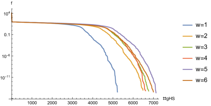
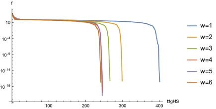
Representative results for single runs are presented in Figs. 1, 2, 3, and 4. At times the algorithm converges to the secondary local min described in [KS09]. These runs are discarded. Figure 1 should be compared to Fig. 2 to see the comparatively slow convergence of the PSB update.

Figure 1: Block PSB with preliminary secant update (i.e., with pflag=1 in Algorithm 5). Supplemental directions chosen using Eq. 9d. Surprisingly, as we increase the sample size, the performance of the algorithm degrades.

Figure 2: Block SR1 with preliminary secant update (i.e., with pflag=1 in Algorithm 5). Supplemental directions chosen using Eq. 9d. Comparing Fig. 2 and Fig. 1, block SR1 converges much more rapidly than block PSB. Also, the convergence of block SR1 is superior for larger sample sizes $w$, though the improvement appears to decrease as $w$ increases.

The block PSB update is very conservative in the sense that it gives the smallest change (in the Frobenius norm) consistent with the new Hessian sample which may cause PSB to struggle with the rapidly changing Rosenbrock Hessian. SR1 is the primary focus from here on. As would be expected Fig. 2 shows SR1 converging faster for larger sample sizes $w$. The improvement appears to decrease as $w$ increases.

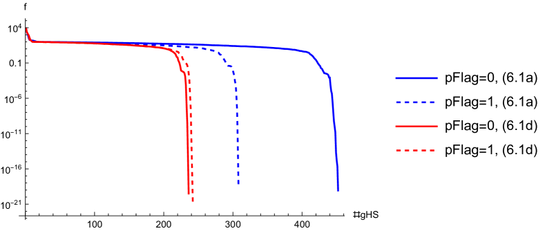
Figure 3 compares several SR1 variants with and without a preliminary secant update (pflag = $\{0,1\}$ in Algorithm 5) and sample directions chosen from $\{$Eqs. 9a and 9d$\}$. The sample size is held fixed at $w=4$. The blue curves (sample directions do not include $p_{k}$, Eq. 9a) are consistent with the observations in [BSS88b, BSS88a] that including the approximate secant curvature information in a preliminary QN update is advantageous. Incorporating $p_{k}$ in our selection of sample directions, Eq. 9d is highly beneficial (red curves), and eliminates the need for the preliminary QN update, which is a serial bottleneck.

Figure 3: Convergence of SR1 variants with pflag=$\{0,1\}$, and sample directions chosen using $\{\lx@cref{creftype~refnum}{eq:SUpdate1},\lx@cref{creftype~refnum}{eq:SUpdate4}\}$. Sample size is held fixed at $w=4$. The blue curves (sample directions do not include $p_{k}$, Eq. 9a) are consistent with the observations in [BSS88b, BSS88a] that including the approximate secant curvature information in a preliminary QN update is advantageous. Our framework allows us to incorporate Hessian information in the direction of $p_{k}$, i.e., Eq. 9d. The red curves show that using Eq. 9d to select sample directions is highly beneficial, and eliminates the need to include approximate secant curvature information in the Hessian, which is a serial bottleneck.

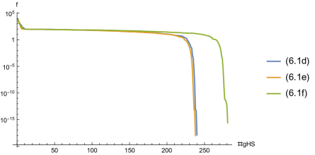
Lastly, Fig. 4 shows the effect of varying the sample selection strategy between Eqs. 9d, 9e, and 9f The simple purely randomized supplemental directions from Eq. 9d gave good results. The intuition behind Eq. 9e was to prevent immediate re-sampling by orthogonalizing against the immediate previous directions. It did not lead to significant improvement. The intuition behind Eq. 9f was to guide the algorithm to accurately resolve eigen-space associated with the larger Hessian eigenvalues. This variant does appear to resolve these eigenspaces but unfortunately it does not improve the performance of the algorithm.

Figure 4: SR1 with with $w=4$, samples from Eqs. 9d, 9e, and 9f, and no preliminary secant update (i.e., with pflag=0 in Algorithm 5). The simple purely randomized supplemental directions from Eq. 9d gave good results.

9 Conclusions and Future Work

The goal was a straightforward algorithm that would focus on potential benefits AD generated Hessian samples in optimization algorithms. The algorithms presented are intended to evaluate potential benefits of incorporating block Hessian samples in various ways into a fairly standard optimization framework. Practical implementations would require limited memory updates to reduce storage requirements. Carefully eliminating some sampled directions from the trust region sub problem and/or exploiting the structure of a limited memory update (as shown for LSR1 by Brust et al. [BEM17]) would reduce the computational intensity of the trust-region sub-problem solver. We do not address these issues in this article and restrict attention to significantly fewer than the $64$ Hessian samples which are feasible on common GPU hardware.

10 Distribution of Responsibilities

The article implements matrix approximation ideas from Dr. Azzam’s thesis in optimization. Dr. Struthers designed the algorithm and drafted the article with significant input from Drs. Ong and Azzam. Mr. Henderson created the Julia test problems and code, and generated numerical results. All authors made significant editorial contributions.

References

- [1]
- [AINT17] Adachi, Satoru ; Iwata, Satoru ; Nakatsukasa, Yuji ; Takeda, Akiko: Solving the Trust-Region Subproblem By a Generalized Eigenvalue Problem. In: SIAM Journal on Optimization 27 (2017), Nr. 1, 269-291. http://dx.doi.org/10.1137/16M1058200. – DOI 10.1137/16M1058200
- [BCN18] Bottou, Léon ; Curtis, Frank E. ; Nocedal, Jorge: Optimization Methods for Large-Scale Machine Learning. In: SIAM Review 60 (2018), Nr. 2, 223-311. http://dx.doi.org/10.1137/16M1080173. – DOI 10.1137/16M1080173
- [BEM17] Brust, Johannes ; Erway, Jennifer B. ; Marcia, Roummel F.: On Solving L-SR1 Trust-Region Subproblems. In: Comput. Optim. Appl. 66 (2017), März, Nr. 2, 245–266. http://dx.doi.org/10.1007/s10589-016-9868-3. – DOI 10.1007/s10589–016–9868–3. – ISSN 0926–6003
- [BJRT21] Berahas, A. S. ; Jahani, M. ; Richtárik, P. ; Takáč, M.: Quasi-Newton methods for machine learning: forget the past, just sample. In: Optimization Methods and Software 0 (2021), Nr. 0, 1-37. http://dx.doi.org/10.1080/10556788.2021.1977806. – DOI 10.1080/10556788.2021.1977806
- [BSS88a] Byrd, R. H. ; Schnabel, R. B. ; Shultz, G. A.: Using Parallel Function Evaluations to Improve Hessian Approximation for Unconstrained Optimization. In: Ann. Oper. Res. 14 (1988), Juni, Nr. 1–4, 167–193. http://dx.doi.org/10.1007/BF02186479. – DOI 10.1007/BF02186479. – ISSN 0254–5330
- [BSS88b] Byrd, R.H. ; Schnabel, R.B. ; Shultz, G.A.: Parallel quasi-Newton methods for unconstrained optimization. In: Mathematical Programming 42 (1988), Nr. 1-3, 273-306. http://dx.doi.org/10.1007/BF01589407. – DOI 10.1007/BF01589407. – cited By 46
- [CGT88] Conn, Andrew ; Gould, Nicholas ; Toint, Philippe: Testing a Class of Methods for Solving Minimization Problems with Simple Bounds on the Variables. In: Mathematics of Computation 50 (1988), 05. http://dx.doi.org/10.2307/2008615. – DOI 10.2307/2008615
- [GG18] Gao, Wenbo ; Goldfarb, Donald: Block BFGS Methods. In: SIAM Journal on Optimization 28 (2018), Nr. 2, 1205-1231. http://dx.doi.org/10.1137/16M1092106. – DOI 10.1137/16M1092106
- [GG19] Gao, Wenbo ; Goldfarb, Donald: Quasi-Newton methods: superlinear convergence without line searches for self-concordant functions. In: Optimization Methods and Software 34 (2019), Nr. 1, 194-217. http://dx.doi.org/10.1080/10556788.2018.1510927. – DOI 10.1080/10556788.2018.1510927
- [HS22] Henderson, P. ; Struthers, A.: BlockOpt: A Julia Package. http://dx.doi.org/10.5281/zenodo.5826808. Version: 2022
- [KS09] Kok, Schalk ; Sandrock, Carl: Locating and Characterizing the Stationary Points of the Extended Rosenbrock Function. In: Evolutionary Computation 17 (2009), 09, Nr. 3, 437-453. http://dx.doi.org/10.1162/evco.2009.17.3.437. – DOI 10.1162/evco.2009.17.3.437. – ISSN 1063–6560
- [MTK03] Migdalas, A. ; Toraldo, G. ; Kumar, V.: Nonlinear optimization and parallel computing. In: Parallel Computing 29 (2003), Nr. 4, 375-391. http://dx.doi.org/https://doi.org/10.1016/S0167-8191(03)00013-9. – DOI https://doi.org/10.1016/S0167–8191(03)00013–9. – ISSN 0167–8191. – Parallel computing in numerical optimization
- [NJN21] N., Rontsis ; J., Goulart P. ; Nakatsukasa, Y.: TRS.jl. https://github.com/oxfordcontrol/TRS.jl. Version: 2021
- [NW06] Nocedal, Jorge ; Wright, Stephen J.: Numerical Optimization. second. New York, NY, USA : Springer, 2006
- [RGN21] Rontsis, Nikitas ; Goulart, Paul ; Nakatsukasa, Yuji: An active-set algorithm for norm constrained quadratic problems. In: Mathematical Programming (2021), 03, S. 1–37. http://dx.doi.org/10.1007/s10107-021-01617-2. – DOI 10.1007/s10107–021–01617–2
- [RLP16] Revels, J. ; Lubin, M. ; Papamarkou, T.: Forward-Mode Automatic Differentiation in Julia. In: arXiv:1607.07892 [cs.MS] (2016). https://arxiv.org/abs/1607.07892
- [Sch87] Schnabel, R.B.: Concurrent function evaluations in local and global optimization. In: Computer Methods in Applied Mechanics and Engineering 64 (1987), Nr. 1-3, 537-552. http://dx.doi.org/10.1016/0045-7825(87)90055-7. – DOI 10.1016/0045–7825(87)90055–7. – cited By 17
- [Sch95] Schnabel, Robert B.: A view of the limitations, opportunities, and challenges in parallel nonlinear optimization. In: Parallel Computing 21 (1995), Nr. 6, 875-905. http://dx.doi.org/https://doi.org/10.1016/0167-8191(95)00004-8. – DOI https://doi.org/10.1016/0167–8191(95)00004–8. – ISSN 0167–8191