Detecting Twenty-thousand Classes
using Image-level Supervision
Abstract
Current object detectors are limited in vocabulary size due to the small scale of detection datasets. Image classifiers, on the other hand, reason about much larger vocabularies, as their datasets are larger and easier to collect. We propose Detic, which simply trains the classifiers of a detector on image classification data and thus expands the vocabulary of detectors to tens of thousands of concepts. Unlike prior work, Detic does not need complex assignment schemes to assign image labels to boxes based on model predictions, making it much easier to implement and compatible with a range of detection architectures and backbones. Our results show that Detic yields excellent detectors even for classes without box annotations. It outperforms prior work on both open-vocabulary and long-tail detection benchmarks. Detic provides a gain of 2.4 mAP for all classes and 8.3 mAP for novel classes on the open-vocabulary LVIS benchmark. On the standard LVIS benchmark, Detic obtains 41.7 mAP when evaluated on all classes, or only rare classes, hence closing the gap in performance for object categories with few samples. For the first time, we train a detector with all the twenty-one-thousand classes of the ImageNet dataset and show that it generalizes to new datasets without finetuning. Code is available at https://github.com/facebookresearch/Detic.
1 Introduction
Object detection consists of two sub-problems - finding the object (localization) and naming it (classification). Traditional methods tightly couple these two sub-problems and thus rely on box labels for all classes. Despite many data collection efforts, detection datasets [34, 18, 49, 28] are much smaller in overall size and vocabularies than classification datasets [10]. For example, the recent LVIS detection dataset [18] has 1000+ classes with 120K images; OpenImages [28] has 500 classes in 1.8M images. Moreover, not all classes contain sufficient annotations to train a robust detector (see Figure 1 Top). In classification, even the ten-year-old ImageNet [10] has 21K classes and 14M images (Figure 1 Bottom).


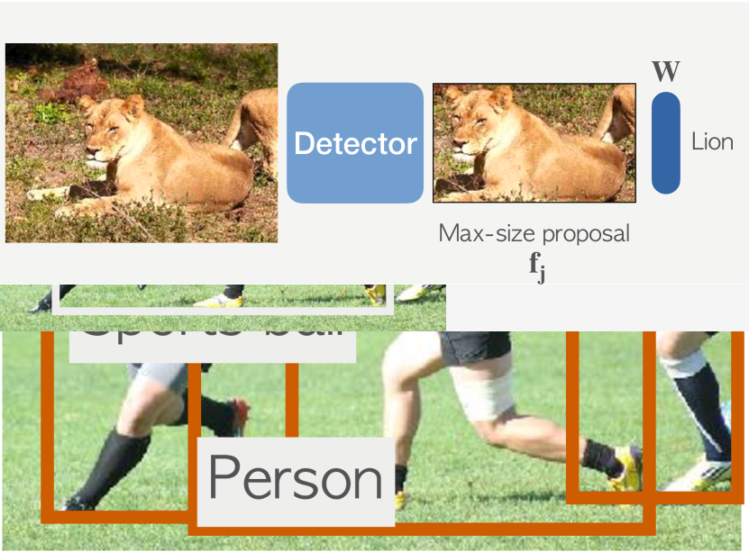
In this paper, we propose Detector with image classes (Detic) that uses image-level supervision in addition to detection supervision. We observe that the localization and classification sub-problems can be decoupled. Modern region proposal networks already localize many ‘new’ objects using existing detection supervision. Thus, we focus on the classification sub-problem and use image-level labels to train the classifier and broaden the vocabulary of the detector. We propose a simple classification loss that applies the image-level supervision to the proposal with the largest size, and do not supervise other outputs for image-labeled data. This is easy to implement and massively expands the vocabulary.
Most existing weakly-supervised detection techniques [59, 22, 13, 67, 36] use the weakly labeled data to supervise both the localization and classification sub-problems of detection. Since image-classification data has no box labels, these methods develop various label-to-box assignment techniques based on model predictions to obtain supervision. For example, YOLO9000[45] and DLWL[44] assign the image label to proposals that have high prediction scores on the labeled class. Unfortunately, this prediction-based assignment requires good initial detections which leads to a chicken-and-egg problem—we need a good detector for good label assignment, but we need many boxes to train a good detector. Our method completely side-steps the prediction-based label assignment process by supervising the classification sub-problem alone when using classification data. This also enables our method to learn detectors for new classes which would have been impossible to predict and assign.
Experiments on the open-vocabulary LVIS [18, 17] and the open-vocabulary COCO [2] benchmarks show that our method can significantly improve over a strong box-supervised baseline, on both novel and base classes. With image-level supervision from ImageNet-21K [10], our model trained without novel class detection annotations improves the baseline by point and matches the performance of using full class annotations in training. With the standard LVIS annotations, our model reaches mAP and mAP, closing the gap between rare classes and all classes. On open-vocabulary COCO, our method outperforms the previous state-of-the-art OVR-CNN [72] by point with the same detector and data. Finally, we train a detector using the full ImageNet-21K with more than twenty-thousand classes. Our detector generalizes much better to new datasets [49, 28] with disjoint label spaces, reaching mAP on Objects365 and mAP50 on OpenImages, without seeing any images from the corresponding training sets. Our contributions are summarized below:
-
•
We identify issues and propose a simpler alternative to existing weakly-supervised detection techniques in the open-vocabulary setting.
-
•
Our proposed family of losses significantly improves detection performance on novel classes, closely matching the supervised performance upper bound.
-
•
Our detector transfers to new datasets and vocabularies without finetuning.
-
•
We release our code (in supplement). It is ready-to-use for open-vocabulary detection in the real world. See examples in supplement.


2 Related Work
Weakly-supervised object detection (WSOD) trains object detector using image-level labels. Many works use only image-level labels without any box supervision [30, 52, 70, 63, 51]. WSDDN [3] and OIRC [60] use a subnetwork to predict per-proposal weighting and sum up proposal scores into a single image scores. PCL [59] first clusters proposals and then assign image labels at the cluster level. CASD [22] further introduces feature-level attention and self-distillation. As no bounding box supervision is used in training, these methods rely on low-level region proposal techniques [62, 1], which leads to reduced localization quality.
Another line of WSOD work uses bounding box supervision together with image labels, known as semi-supervised WSOD [68, 13, 61, 31, 35, 75, 12]. YOLO9000 [45] mixes detection data and classification data in the same mini-batch, and assigns classification labels to anchors with the highest predicted scores. DLWL [44] combines self-training and clustering-based WSOD [59], and again assigns image labels to max-scored proposals. MosaicOS [73] handles domain differences between detection and image datasets by mosaic augmentation [4] and proposed a three-stage self-training and finetuning framework. In segmentation, Pinheiro et al. [41] use a log-sum-exponential function to aggregate pixels scores into a global classification. Our work belongs to semi-supervised WSOD. Unlike prior work, we use a simple image-supervised loss. Besides image labels, researchers have also studied complementary methods for weak localization supervision like points [7] or scribles [47].
Open-vocabulary object detection, or also named zero-shot object detection, aims to detect objects outside of the training vocabulary. The basic solution [2] is to replace the last classification layer with language embeddings (e.g., GloVe [40]) of the class names. Rahman et al. [43] and Li et al. [33] improve the classifier embedding using external text information. OVR-CNN [72] pretrains the detector on image-text pairs. ViLD [17], OpenSeg [16] and langSeg [29] upgrade the language embedding to CLIP [42]. ViLD further distills region features from CLIP image features. We use CLIP [42] classifier as well, but do not use distillation. Instead, we use additional image-labeled data for co-training.
Large-vocabulary object detection [18, 69, 53, 45] requires detecting 1000+ classes. Many existing works focus on handling the long-tail problem [39, 32, 74, 65, 14, 6]. Equalization losses [56, 55] and SeeSaw loss [64] reweights the per-class loss by balancing the gradients [55] or number of samples [64]. Federated Loss [76] subsamples classes per-iteration to mimic the federated annotation [18]. Yang et al. [69] detects 11K classes with a label hierarchy. Our method builds on these advances, and we tackle the problem from a different aspect: using additional image-labeled data.
Proposal Network Generalization. ViLD [17] reports that region proposal networks have certain generalization abilities for new classes by default. Dave et al. [9] shows segmentation and localization generalizes across classes. Kim et al. [25] further improves proposal generalization with a localization quality estimator. In our experiments, we found proposals to generalize well enough (see Appendix 0.A), as also observed in ViLD [17]. Further improvements to RPNs [17, 25, 27, 38] can hopefully lead to better results.
3 Preliminaries
We train object detectors using both object detection and image classification datasets. We propose a simple way to leverage image supervision to learn object detectors, including for classes without box labels. We first describe the object detection problem and then detail our approach.
Problem setup. Given an image , object detection solves the two subproblems of (1) localization: find all objects with their location, represented as a box and (2) classification: assign a class label to the -th object. Here is the class vocabulary provided by the user at test time. During training, we use a detection dataset with vocabulary that has both class and box labels. We also use an image classification dataset with vocabulary that only has image-level class labels. The vocabularies , , may or may not overlap.
Traditional Object detection considers and . Predominant object detectors [46, 20] follow a two-stage framework. The first stage, called the region proposal network (RPN), takes the image and produces a set of object proposals , where is a -dimensional region feature and is the objectness score. The second stage takes the object feature and outputs a classification score and a refined box location for each object, , , where and are the learned weights of the classification layer and the regression layer, respectively.111We omit the two linear layers and the bias in the second stage for notation simplicity. Our work focuses on improving classification in the second stage. In our experiments, the proposal network and the bounding box regressors are not the current performance bottleneck, as modern detectors use an over-sufficient number of proposals in testing (1K proposals for 20 objects per image. see Appendix 0.A for more details).
Open-vocabulary object detection allows . Simply replacing the classification weights with fixed language embeddings of class names converts a traditional detector to an open-vocabulary detector [2]. The region features are trained to match the fixed language embeddings. We follow Gu et al. [17] to use the CLIP embeddings [42] as the classification weights. In theory, this open-vocabulary detector can detect any object class. However, in practice, it yields unsatisfying results as shown in Figure 1. Our method uses image-level supervision to improve object detection including in the open-vocabulary setting.


4 Detic: Detector with Image Classes
As shown in Figure 3, our method leverages the box labels from detection datasets and image-level labels from classification datasets . During training, we compose a mini-batch using images from both types of datasets. For images with box labels, we follow the standard two-stage detector training [46]. For image-level labeled images, we only train the features from a fixed region proposal for classification. Thus, we only compute the localization losses (RPN loss and bounding box regression loss) on images with ground truth box labels. Below we describe our modified classification loss for image-level labels.
A sample from the weakly labeled dataset contains an image and a set of labels . We use the region proposal network to extract object features . Prediction-based methods try to assign image labels to regions, and aim to train both localization and classification abilities. Instead, we propose simple ways to use the image labels and only improve classification. Our key idea is to use a fixed way to assign image labels to regions, and side-step a complex prediction-based assignment. We allow the fixed assignment schemes miss certain objects, as long as they miss fewer objects than the prediction-based counterparts, thus leading to better performance.
Non-prediction-based losses. We now describe a variety of simple ways to use image labels and evaluate them empirically in Table 1. Our first idea is to use the whole image as a new “proposal” box. We call this loss image-box. We ignore all proposals from the RPN, and instead use an injected box of the whole image . We then apply the classification loss to its RoI features for all classes :
where is the binary cross-entropy loss, and is the sigmoid activation. Thus, our loss uses the features from the same ‘proposal’ for solving the classification problem for all the classes .
In practice, the image-box can be replaced by smaller boxes. We introduce two alternatives: the proposal with the max object score or the proposal with the max size:
We show that all these three losses can effectively leverage the image-level supervision, while the max-size loss performs the best. We thus use the max-size loss by default for image-supervised data. We also note that the classification parameters are shared across both detection and classification data, which greatly improves detection performance. The overall training objective is
where , , are standard losses in a two-stage detector, and is the weight of our loss.
Relation to prediction-based assignments. In traditional weakly-supervised detection [3, 45, 44], a popular idea is to assign the image to the proposals based on model prediction. Let be the stacked feature of all object proposals and be their classification scores. For each , , where is the label-to-box assignment process. In most methods, is a function of the prediction . For example, selects the proposal with max score on . Our key insight is that should not depend on the prediction . In large-vocabulary detection, the initial recognition ability of rare or novel classes is low, making the label assignment process inaccurate. Our method side-steps this prediction-and-assignment process entirely and relies on a fixed supervision criteria.
5 Experiments
We evaluate Detic on the large-vocabulary object detection dataset LVIS [18]. We mainly use the open-vocabulary setting proposed by Gu et al. [17], and also report results on the standard LVIS setting. We describe our experiment setup below.
LVIS. The LVIS [18] dataset has object detection and instance segmentation labels for classes with 100K images. The classes are divided into three groups - frequent, common, rare based on the number of training images. We refer to this standard LVIS training set as LVIS-all. Following ViLD [17], we remove the labels of rare-class from training and consider them as novel classes in testing. We refer to this partial training set with only frequent and common classes as LVIS-base. We report mask mAP which is the official metric for LVIS. While our model is developed for box detection, we use a standard class-agnostic mask head [20] to produce segmentation masks for boxes. We train the mask head only on detection data.
Image-supervised data. We use two sources of image-supervised data: ImageNet-21K [10] and Conceptual Captions [50]. ImageNet-21K (IN-21K) contains 14M images for 21K classes. For ease of training and evaluation, most of our experiments use the 997 classes that overlap with the LVIS vocabulary and denote this subset as IN-L. Conceptual Captions [50] (CC) is an image captioning dataset containing 3M images. We extract image labels from the captions using exact text-matching and keep images whose captions mention at least one LVIS class. See Appendix 0.B for results of directly using captions. The resulting dataset contains 1.5M images with 992 LVIS classes. We summarize the datasets used below.
| Notation | Definition | #Images | #Classes |
| LVIS-all | The original LVIS dataset [18] | 100K | 1203 |
| LVIS-base | LVIS without rare-class annotations | 100K | 866 |
| IN-21K | The original ImageNet-21K dataset [10] | 14M | 21k |
| IN-L | 997 overlapping IN-21K classes with LVIS | 1.2M | 997 |
| CC | Conceptual Captions [50] with LVIS classes | 1.5M | 992 |
5.1 Implementation details
Box-Supervised: a strong LVIS baseline. We first establish a strong baseline on LVIS to demonstrate that our improvements are orthogonal to recent advances in object detection. The baseline only uses the supervised bounding box labels. We use the CenterNet2 [76] detector with ResNet50 [21] backbone. We use Federated Loss [76] and repeat factor sampling [18]. We use large scale jittering [15] with input resolution and train for a ( LVIS epochs) schedule. To show our method is compatible with better pretraining, we use ImageNet-21k pretrained backbone weights [48]. As described in § 3, we use the CLIP [42] embedding as the classifier. Our baseline is mAP higher than the detectron2 baseline [66] ( vs. mAP) and trains in a similar time (17 vs. 12 hours on 8 V100 GPUs). See Appendix 0.C for more details.
Resolution change for image-labeled images. ImageNet images are inherently smaller and more object-focused than LVIS images [73]. In practice, we observe it is important to use smaller image resolution for ImageNet images. Using smaller resolution in addition allows us to increase the batch-size with the same computation. In our implementation, we use for ImageNet and CC and ablate this in Appendix 0.D.
Multi-dataset training. We sample detection and classification mini-batches in a ratio, regardless of the original dataset size. We group images from the same dataset on the same GPU to improve training efficiency [77].
Training schedules. To shorten the experimental cycle and have a good initialization for prediction-based WSOD losses [44, 45], we always first train a converged base-class-only model ( schedule) and finetune on it with additional image-labeled data for another schedule. We confirm finetuning the model using only box supervision does not improve the performance. The schedule for our joint training consists of LVIS epochs plus ImageNet epochs or CC epochs. Training our ResNet50 model takes hours on 8 V100 GPUs. The large 21K Swin-B model trains in hours on 32 GPUs.
5.2 Prediction-based vs non-prediction-based methods
Table 1 shows the results of the box-supervised baseline, existing prediction-based methods, and our proposed non-prediction-based methods. The baseline (Box-Supervised) is trained without access to novel class bounding box labels. It uses the CLIP classifier [17] and has open-vocabulary capabilities with 16.3 mAP. In order to leverage additional image-labeled data like ImageNet or CC, we use prior prediction-based methods or our non-prediction-based method.
We compare a few prediction-based methods that assign image labels to proposals based on predictions. Self-training assigns predictions of Box-Supervised as pseudo-labels offline with a fixed score threshold (). The other prediction-based methods use different losses to assign predictions to image labels online. See Appendix 0.E for implementation details. For DLWL [44], we implement a simplified version that does not include bootstrapping and refer to it as DLWL*.
| IN-L (object-centric) | CC (non object-centric) | ||||
| mAP | mAP | mAP | mAP | ||
| Box-Supervised (baseline) | 30.0 | 16.3 | 30.0 | 16.3 | |
| Prediction-based methods | |||||
| Self-training [54] | 30.3 | 15.6 | 30.1 | 15.9 | |
| WSDDN [3] | 29.8 | 15.6 | 30.0 | 16.5 | |
| DLWL* [44] | 30.6 | 18.2 | 29.7 | 16.9 | |
| YOLO9000 [45] | 31.2 | 20.4 | 29.4 | 15.9 | |
| Non-prediction-based methods | |||||
| Detic (Max-object-score) | 32.2 | 24.4 | 29.8 | 18.2 | |
| Detic (Image-box) | 32.4 | 23.8 | 30.9 | 19.5 | |
| Detic (Max-size) | 32.4 | 24.6 | 30.9 | 19.5 | |
| Fully-supervised (all classes) | 31.1 | 25.5 | 31.1 | 25.5 | |
Table 1 (third block) shows the results of our non-prediction-based methods in § 4. All variants of our proposed simpler method outperform the complex prediction-based counterparts, with both image-supervised datasets. On the novel classes, Detic provides a significant gain of points with ImageNet over the best prediction-based methods.
Using non-object centric images from Conceptual Captions. ImageNet images typically have a single large object [18]. Thus, our non-prediction-based methods, for example image-box which considers the entire image as a bounding box, are well suited for ImageNet. To test whether our losses work with different image distributions with multiple objects, we test it with the Conceptual Captions (CC) dataset. Even on this challenging dataset with multiple objects/labels per image, Detic provides a gain of points on novel class detection over the best prediction-based methods. This suggests that our simpler Detic method can generalize to different types of image-labeled data. Overall, the results from Table 1 suggest that complex prediction-based methods that overly rely on model prediction scores do not perform well for open-vocabulary detection. Amongst our non-prediction-based variants, the max-size loss consistently performs the best, and is the default for Detic in our following experiments.
Why does max-size work? Intuitively, our simpler non-prediction methods outperform the complex prediction-based method by side-stepping a hard assignment problem. Prediction-based methods rely on strong initial detections to assign image-level labels to predicted boxes. When the initial predictions are reliable, prediction-based methods are ideal. However, in open-vocabulary scenarios, such strong initial predictions are absent, which explains the limited performance of prediction-based methods. Detic’s simpler assignment does not rely on strong predictions and is more robust under the challenges of open-vocabulary setting.
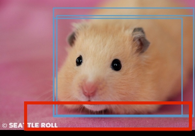
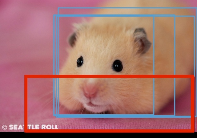
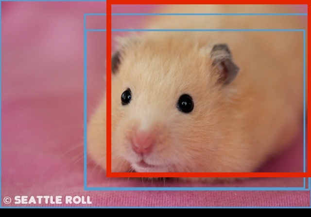
We now study two additional advantages of the Detic max-size variant over prediction-based methods that may contribute to improved performance: 1) the selected max-size proposal can safely cover the target object; 2) the selected max-size proposal is consistent during different training iterations.
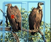
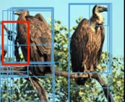
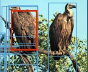
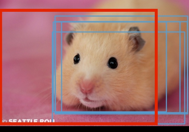
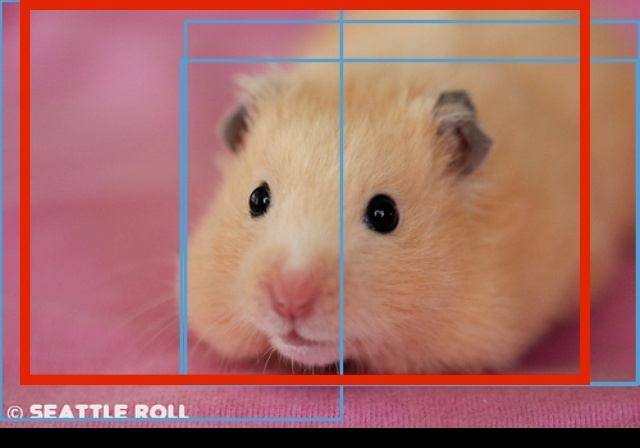
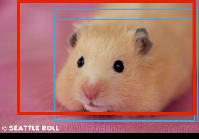
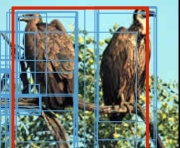
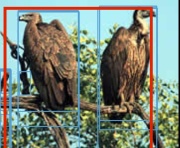
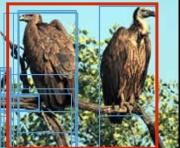
Figure 4 provides typical qualitative examples of the assigned region for the prediction-based method and our max-size variant. On an annotated subset of IN-L, Detic max-size covers target objects, vs. for the prediction-based method. Overall, unlike prediction-based methods, Detic’s simpler assignment yields boxes that are more likely to contain the object. Indeed, Detic may miss certain objects (especially small objects) or supervise to a loose region. However, in order for Detic to yield a good detector, the selected box need not be perfect, it just needs to 1) provide meaningful training signal (cover the objects and be consistent during training); 2) be ‘more correct’ than the box selected by the prediction-based method. We provide details about our metrics, more quantitative evaluation, and more discussions in Appendix 0.F.
| iters | iters | Convergence | iters | iters | Convergence | |
|
Pred.-based |
 |
 |
 |
 |
 |
 |
|
Max-size |
 |
 |
 |
 |
 |
 |
| mAP | mAP | mAP | mAP | |
| ViLD-text [17] | 24.9 | 10.1 | 23.9 | 32.5 |
| ViLD [17] | 22.5 | 16.1 | 20.0 | 28.3 |
| ViLD-ensemble [17] | 25.5 | 16.6 | 24.6 | 30.3 |
| Detic | 26.8 | 17.8 | 26.3 | 31.6 |
5.3 Comparison with a fully-supervised detector
In Table 1, compared with the strong baseline Box-Supervised, Detic improves the detection performance by mAP and mAP. Thus, Detic with image-level labels leads to strong open-vocabulary detection performance and can provide orthogonal gains to existing open-vocabulary detectors [2]. To further understand the open-vocabulary capabilities of Detic, we also report the top-line results trained with box labels for all classes (Table 1 last row). Despite not using box labels for the novel classes, Detic with ImageNet performs favorably compared to the fully-supervised detector. This result also suggests that bounding box annotations may not be required for new classes. Detic combined with large image classification datasets is a simple and effective alternative for increasing detector vocabulary.
5.4 Comparison with the state-of-the-art
We compare Detic’s open-vocabulary object detectors with state-of-the-art methods on the open-vocabulary LVIS and the open-vocabulary COCO benchmarks. In each case, we strictly follow the architecture and setup from prior work to ensure fair comparisons.
Open-vocabulary LVIS. We compare to ViLD [17], which first uses CLIP embeddings [42] for open-vocabulary detection. We strictly follow their training setup and model architecture (Appendix 0.G) and report results in Table 2. Here ViLD-text is exactly our Box-Supervised baseline. Detic provides a gain of points on mAP. Compared to ViLD-text, ViLD, which uses knowledge distillation from the CLIP visual backbone, improves mAP at the cost of hurting overall mAP. Ensembling the two models, ViLD-ens provides improvements for both metrics. On the other hand, Detic uses a single model which improves both novel and overall mAP, and outperforms the ViLD ensemble.
Open-vocabulary COCO. Next, we compare with prior works on the popular open-vocabulary COCO benchmark [2] (see benchmark and implementation details in Appendix 0.H). We strictly follow OVR-CNN [72] to use Faster R-CNN with ResNet50-C4 backbone and do not use any improvements from § 5.1. Following [72], we use COCO captions as the image-supervised data. We extract nouns from the captions and use both the image labels and captions as supervision.
| mAP50 | mAP50 | mAP50 | |
| Base-only† | 39.9 | 0 | 49.9 |
| Base-only (CLIP) | 39.3 | 1.3 | 48.7 |
| WSDDN [3]† | 24.6 | 20.5 | 23.4 |
| Cap2Det [71]† | 20.1 | 20.3 | 20.1 |
| SB [2]‡ | 24.9 | 0.31 | 29.2 |
| DELO [78]‡ | 13.0 | 3.41 | 13.8 |
| PL [43]‡ | 27.9 | 4.12 | 35.9 |
| OVR-CNN [72]† | 39.9 | 22.8 | 46.0 |
| Detic | 45.0 | 27.8 | 47.1 |
Table 3 summarizes our results. As the training set contains only 48 base classes, the base-class only model (second row) yields low mAP on novel classes. Detic improves the baseline and outperforms OVR-CNN [72] by a large margin, using exactly the same model, training recipe, and data.
Additionally, similar to Table 1, we compare to prior prediction-based methods on the open-vocabulary COCO benchmark in Appendix 0.H. In this setting too, Detic improves over prior work providing significant gains on novel class detection and overall detection performance.
5.5 Detecting 21K classes across datasets without finetuning
Next, we train a detector with the full 21K classes of ImageNet. We use our strong recipe with Swin-B [37] backbone. In practice, training a classification layer of 21K classes is computationally involved.222This is more pronounced in detection than classification, as the “batch-size” for the classification layer is image-batch-size, where is #RoIs per image. We adopt a modified Federated Loss [76] that uniformly samples classes from the vocabulary at every iteration. We only compute classification scores and back-propagate on the sampled classes.
| Objects365 [49] | OpenImages [28] | |||
| mAP | mAP | mAP50 | mAP50 | |
| Box-Supervised | 19.1 | 14.0 | 46.2 | 61.7 |
| Detic w. IN-L | 21.2 | 17.8 | 53.0 | 67.1 |
| Detic w. IN-21k | 21.5 | 20.0 | 55.2 | 68.8 |
| Dataset-specific oracles | 31.2 | 22.5 | 69.9 | 81.8 |
 |
 |
 |
 |
 |
 |
 |
 |
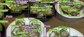
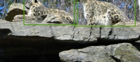
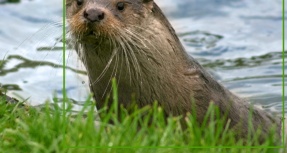
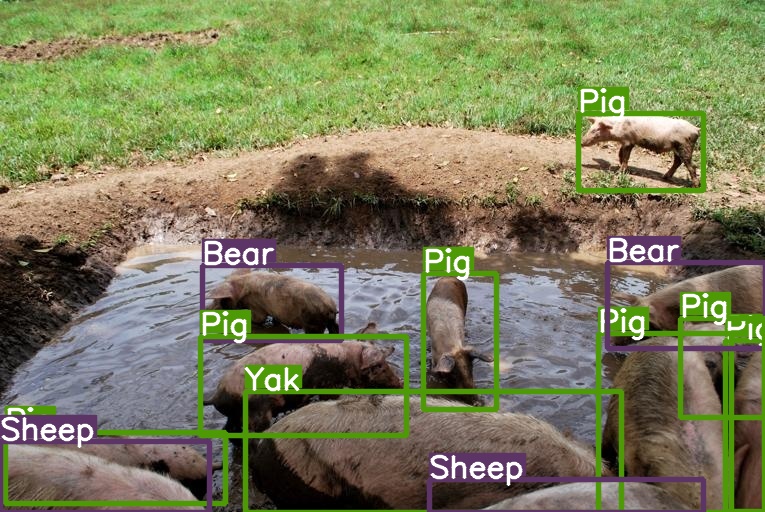
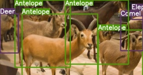
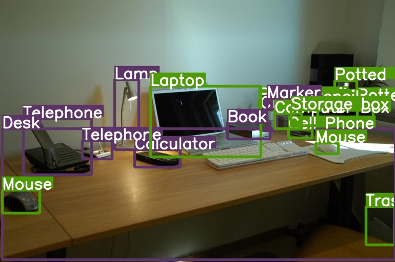
As there are no direct benchmark to evaluate detectors with such large vocabulary, we evaluate our detectors on new datasets without finetuning. We evaluate on two large-scale object detection datasets: Objects365v2 [49] and OpenImages [28], both with around M training images. We follow LVIS to split of classes with the fewest training images as rare classes. Table 4 shows the results. On both datasets, Detic improves the Box-Supervised baseline by a large margin, especially on classes with fewer annotations. Using all the 21k classes further improves performance owing to the large vocabulary. Our single model significantly reduces the gap towards the dataset-specific oracles and reaches - of their performance without using the corresponding M detection annotations. See Figure 5 for qualitative results.
5.6 Ablation studies
We now ablate our key components under the open-vocabulary LVIS setting with IN-L as the image-classification data. We use our strong training recipe as described in § 5.1 for all these experiments.
| Box-Supervised | Detic | |||
| Classifier | mAP | mAP | mAP | mAP |
| *CLIP [42] | 30.2 | 16.4 | 32.4 | 24.9 |
| Trained | 27.4 | 0 | 31.7 | 17.4 |
| FastText [24] | 27.5 | 9.0 | 30.9 | 19.2 |
| OpenCLIP [23] | 27.1 | 8.9 | 30.7 | 19.4 |
Classifier weights. We study the effect of different classifier weights . While our main open-vocabulary experiments use CLIP [42], we show the gain of Detic is independent of CLIP. We train Box-Supervised and Detic with different classifiers, including a standard random initialized and trained classifier, and other fixed language models [24, 23] The results are shown in Table 5. By default, a trained classifier cannot recognize novel classes. However, Detic enables novel class recognition ability even in this setting ( mAP for classes without detection labels). Using language models such as FastText [24] or an open-source version of CLIP [23] leads to better novel class performance. CLIP [42] performs the best among them.
| Pretrain data | mAP | mAP | |
| Box-Supervised | IN-1K | 26.1 | 13.6 |
| Detic | IN-1K | 28.8 (+2.7) | 21.7 (+8.1) |
| Box-Supervised | IN-21K | 30.2 | 16.4 |
| Detic | IN-21K | 32.4 (+2.2) | 24.9 (+8.5) |
Effect of Pretraining. Many existing methods use additional data only for pretraining [73, 72, 11], while we use image-labeled data for co-training. We present results of Detic with different types of pretraining in Table 6. Detic provides similar gains across different types of pretraining, suggesting that our gains are orthogonal to advances in pretraining. We believe that this is because pretraining improves the overall features, while Detic uses co-training which improves both the features and the classifier.
5.7 The standard LVIS benchmark
Finally, we evaluate Detic on the standard LVIS benchmark [18]. In this setting, the baseline (Box-Supervised) is trained with box and mask labels for all classes while Detic uses additional image-level labels from IN-L. We train Detic with the same recipe in § 5.1 and use a strong Swin-B [37] backbone and input size. We report the mask mAP across all classes and also split into rare, common, and frequent classes. Notably, Detic achieves mAP and mAP, closing the gap between the overall mAP and the rare mAP. This suggests Detic effectively uses image-level labels to improve the performance of classes with very few boxes labels. Appendix 0.I provides more comparisons to prior work [73] on LVIS. Appendix 0.J shows Detic generalizes to DETR-based [79] detectors.
| Backbone | mAP | mAP | mAP | mAP | |
| MosaicOS [73] | ResNeXt-101 | 28.3 | 21.7 | 27.3 | 32.4 |
| CenterNet2 [76] | ResNeXt-101 | 34.9 | 24.6 | 34.7 | 42.5 |
| AsyncSLL [19] | ResNeSt-269 | 36.0 | 27.8 | 36.7 | 39.6 |
| SeesawLoss [64] | ResNeSt-200 | 37.3 | 26.4 | 36.3 | 43.1 |
| Copy-paste [15] | EfficientNet-B7 | 38.1 | 32.1 | 37.1 | 41.9 |
| Tan et al. [57] | ResNeSt-269 | 38.8 | 28.5 | 39.5 | 42.7 |
| Baseline | Swin-B | 40.7 | 35.9 | 40.5 | 43.1 |
| Detic | Swin-B | 41.7 | 41.7 | 40.8 | 42.6 |
6 Limitations and Conclusions
We present Detic which is a simple way to use image supervision in large-vocabulary object detection. While Detic is simpler than prior assignment-based weakly-supervised detection methods, it supervises all image labels to the same region and does not consider overall dataset statistics. We leave incorporating such information for future work. Moreover, open vocabulary generalization has no guarantees on extreme domains. Our experiments show Detic improves large-vocabulary detection with various weak data sources, classifiers, detector architectures, and training recipes.
Acknowledgments. We thank Bowen Cheng and Ross Girshick for helpful discussions and feedback. This material is in part based upon work supported by the National Science Foundation under Grant No. IIS-1845485 and IIS-2006820. Xingyi is supported by a Facebook PhD Fellowship.
References
- [1] Arbeláez, P., Pont-Tuset, J., Barron, J.T., Marques, F., Malik, J.: Multiscale combinatorial grouping. In: CVPR (2014)
- [2] Bansal, A., Sikka, K., Sharma, G., Chellappa, R., Divakaran, A.: Zero-shot object detection. In: ECCV (2018)
- [3] Bilen, H., Vedaldi, A.: Weakly supervised deep detection networks. In: CVPR (2016)
- [4] Bochkovskiy, A., Wang, C.Y., Liao, H.Y.M.: Yolov4: Optimal speed and accuracy of object detection. arXiv:2004.10934 (2020)
- [5] Cai, Z., Vasconcelos, N.: Cascade r-cnn: Delving into high quality object detection. In: CVPR (2018)
- [6] Chang, N., Yu, Z., Wang, Y.X., Anandkumar, A., Fidler, S., Alvarez, J.M.: Image-level or object-level? a tale of two resampling strategies for long-tailed detection. ICML (2021)
- [7] Chen, L., Yang, T., Zhang, X., Zhang, W., Sun, J.: Points as queries: Weakly semi-supervised object detection by points. In: CVPR (2021)
- [8] Dave, A., Dollár, P., Ramanan, D., Kirillov, A., Girshick, R.: Evaluating large-vocabulary object detectors: The devil is in the details. arXiv:2102.01066 (2021)
- [9] Dave, A., Tokmakov, P., Ramanan, D.: Towards segmenting anything that moves. In: ICCVW (2019)
- [10] Deng, J., Dong, W., Socher, R., Li, L.J., Li, K., Fei-Fei, L.: Imagenet: A large-scale hierarchical image database. In: CVPR (2009)
- [11] Desai, K., Johnson, J.: VirTex: Learning Visual Representations from Textual Annotations. In: CVPR (2021)
- [12] Dong, B., Huang, Z., Guo, Y., Wang, Q., Niu, Z., Zuo, W.: Boosting weakly supervised object detection via learning bounding box adjusters. In: ICCV (2021)
- [13] Fang, S., Cao, Y., Wang, X., Chen, K., Lin, D., Zhang, W.: Wssod: A new pipeline for weakly-and semi-supervised object detection. arXiv:2105.11293 (2021)
- [14] Feng, C., Zhong, Y., Huang, W.: Exploring classification equilibrium in long-tailed object detection. In: ICCV (2021)
- [15] Ghiasi, G., Cui, Y., Srinivas, A., Qian, R., Lin, T.Y., Cubuk, E.D., Le, Q.V., Zoph, B.: Simple copy-paste is a strong data augmentation method for instance segmentation. In: CVPR (2021)
- [16] Ghiasi, G., Gu, X., Cui, Y., Lin, T.Y.: Open-vocabulary image segmentation. arXiv:2112.12143 (2021)
- [17] Gu, X., Lin, T.Y., Kuo, W., Cui, Y.: Open-vocabulary object detection via vision and language knowledge distillation. ICLR (2022)
- [18] Gupta, A., Dollar, P., Girshick, R.: LVIS: A dataset for large vocabulary instance segmentation. In: CVPR (2019)
- [19] Han, J., Niu, M., Du, Z., Wei, L., Xie, L., Zhang, X., Tian, Q.: Joint coco and lvis workshop at eccv 2020: Lvis challenge track technical report: Asynchronous semi-supervised learning for large vocabulary instance segmentation (2020)
- [20] He, K., Gkioxari, G., Dollar, P., Girshick, R.: Mask r-cnn. In: ICCV (2017)
- [21] He, K., Zhang, X., Ren, S., Sun, J.: Deep residual learning for image recognition. In: CVPR (2016)
- [22] Huang, Z., Zou, Y., Bhagavatula, V., Huang, D.: Comprehensive attention self-distillation for weakly-supervised object detection. NeurIPS (2020)
- [23] Ilharco, G., Wortsman, M., Carlini, N., Taori, R., Dave, A., Shankar, V., Namkoong, H., Miller, J., Hajishirzi, H., Farhadi, A., Schmidt, L.: Openclip (Jul 2021). https://doi.org/10.5281/zenodo.5143773, https://doi.org/10.5281/zenodo.5143773
- [24] Joulin, A., Grave, E., Bojanowski, P., Douze, M., Jégou, H., Mikolov, T.: Fasttext. zip: Compressing text classification models. arXiv:1612.03651 (2016)
- [25] Kim, D., Lin, T.Y., Angelova, A., Kweon, I.S., Kuo, W.: Learning open-world object proposals without learning to classify. arXiv:2108.06753 (2021)
- [26] Kingma, D.P., Ba, J.: Adam: A method for stochastic optimization. ICLR (2015)
- [27] Konan, S., Liang, K.J., Yin, L.: Extending one-stage detection with open-world proposals. arXiv:2201.02302 (2022)
- [28] Kuznetsova, A., Rom, H., Alldrin, N., Uijlings, J., Krasin, I., Pont-Tuset, J., Kamali, S., Popov, S., Malloci, M., Kolesnikov, A., et al.: The open images dataset v4. IJCV (2020)
- [29] Li, B., Weinberger, K.Q., Belongie, S., Koltun, V., Ranftl, R.: Language-driven semantic segmentation. ICLR (2022)
- [30] Li, X., Kan, M., Shan, S., Chen, X.: Weakly supervised object detection with segmentation collaboration. In: ICCV (2019)
- [31] Li, Y., Zhang, J., Huang, K., Zhang, J.: Mixed supervised object detection with robust objectness transfer. TPAMI (2018)
- [32] Li, Y., Wang, T., Kang, B., Tang, S., Wang, C., Li, J., Feng, J.: Overcoming classifier imbalance for long-tail object detection with balanced group softmax. In: CVPR (2020)
- [33] Li, Z., Yao, L., Zhang, X., Wang, X., Kanhere, S., Zhang, H.: Zero-shot object detection with textual descriptions. In: AAAI (2019)
- [34] Lin, T.Y., Maire, M., Belongie, S., Hays, J., Perona, P., Ramanan, D., Dollár, P., Zitnick, C.L.: Microsoft coco: Common objects in context. In: ECCV (2014)
- [35] Liu, Y., Zhang, Z., Niu, L., Chen, J., Zhang, L.: Mixed supervised object detection by transferringmask prior and semantic similarity. In: NeurIPS (2021)
- [36] Liu, Y.C., Ma, C.Y., He, Z., Kuo, C.W., Chen, K., Zhang, P., Wu, B., Kira, Z., Vajda, P.: Unbiased teacher for semi-supervised object detection. ICLR (2021)
- [37] Liu, Z., Lin, Y., Cao, Y., Hu, H., Wei, Y., Zhang, Z., Lin, S., Guo, B.: Swin transformer: Hierarchical vision transformer using shifted windows. ICCV (2021)
- [38] Maaz, M., Rasheed, H., Khan, S., Khan, F.S., Anwer, R.M., Yang, M.H.: Multi-modal transformers excel at class-agnostic object detection. arXiv:2111.11430 (2021)
- [39] Pan, T.Y., Zhang, C., Li, Y., Hu, H., Xuan, D., Changpinyo, S., Gong, B., Chao, W.L.: On model calibration for long-tailed object detection and instance segmentation. NeurIPS (2021)
- [40] Pennington, J., Socher, R., Manning, C.D.: Glove: Global vectors for word representation. In: EMNLP (2014)
- [41] Pinheiro, P.O., Collobert, R.: Weakly supervised semantic segmentation with convolutional networks. In: CVPR (2015)
- [42] Radford, A., Kim, J.W., Hallacy, C., Ramesh, A., Goh, G., Agarwal, S., Sastry, G., Askell, A., Mishkin, P., Clark, J., et al.: Learning transferable visual models from natural language supervision. arXiv:2103.00020 (2021)
- [43] Rahman, S., Khan, S., Barnes, N.: Improved visual-semantic alignment for zero-shot object detection. In: AAAI (2020)
- [44] Ramanathan, V., Wang, R., Mahajan, D.: Dlwl: Improving detection for lowshot classes with weakly labelled data. In: CVPR (2020)
- [45] Redmon, J., Farhadi, A.: Yolo9000: better, faster, stronger. In: CVPR (2017)
- [46] Ren, S., He, K., Girshick, R., Sun, J.: Faster r-cnn: Towards real-time object detection with region proposal networks. NIPS (2015)
- [47] Ren, Z., Yu, Z., Yang, X., Liu, M.Y., Schwing, A.G., Kautz, J.: Ufo2: A unified framework towards omni-supervised object detection. In: ECCV (2020)
- [48] Ridnik, T., Ben-Baruch, E., Noy, A., Zelnik-Manor, L.: Imagenet-21k pretraining for the masses. In: NeurIPS (2021)
- [49] Shao, S., Li, Z., Zhang, T., Peng, C., Yu, G., Zhang, X., Li, J., Sun, J.: Objects365: A large-scale, high-quality dataset for object detection. In: ICCV (2019)
- [50] Sharma, P., Ding, N., Goodman, S., Soricut, R.: Conceptual captions: A cleaned, hypernymed, image alt-text dataset for automatic image captioning. In: ACL (2018)
- [51] Shen, Y., Ji, R., Wang, Y., Chen, Z., Zheng, F., Huang, F., Wu, Y.: Enabling deep residual networks for weakly supervised object detection. In: ECCV (2020)
- [52] Shen, Y., Ji, R., Wang, Y., Wu, Y., Cao, L.: Cyclic guidance for weakly supervised joint detection and segmentation. In: CVPR (2019)
- [53] Singh, B., Li, H., Sharma, A., Davis, L.S.: R-fcn-3000 at 30fps: Decoupling detection and classification. In: CVPR (2018)
- [54] Sohn, K., Zhang, Z., Li, C.L., Zhang, H., Lee, C.Y., Pfister, T.: A simple semi-supervised learning framework for object detection. arXiv:2005.04757 (2020)
- [55] Tan, J., Lu, X., Zhang, G., Yin, C., Li, Q.: Equalization loss v2: A new gradient balance approach for long-tailed object detection. In: CVPR (2021)
- [56] Tan, J., Wang, C., Li, B., Li, Q., Ouyang, W., Yin, C., Yan, J.: Equalization loss for long-tailed object recognition. In: CVPR (2020)
- [57] Tan, J., Zhang, G., Deng, H., Wang, C., Lu, L., Li, Q., Dai, J.: 1st place solution of lvis challenge 2020: A good box is not a guarantee of a good mask. arXiv:2009.01559 (2020)
- [58] Tan, M., Pang, R., Le, Q.V.: Efficientdet: Scalable and efficient object detection. In: CVPR (2020)
- [59] Tang, P., Wang, X., Bai, S., Shen, W., Bai, X., Liu, W., Yuille, A.: Pcl: Proposal cluster learning for weakly supervised object detection. TPAMI (2018)
- [60] Tang, P., Wang, X., Bai, X., Liu, W.: Multiple instance detection network with online instance classifier refinement. In: CVPR (2017)
- [61] Uijlings, J., Popov, S., Ferrari, V.: Revisiting knowledge transfer for training object class detectors. In: CVPR (2018)
- [62] Uijlings, J.R., Van De Sande, K.E., Gevers, T., Smeulders, A.W.: Selective search for object recognition. IJCV (2013)
- [63] Wan, F., Liu, C., Ke, W., Ji, X., Jiao, J., Ye, Q.: C-mil:continuation multiple instance learning for weakly supervised object detection. In: CVPR (2019)
- [64] Wang, J., Zhang, W., Zang, Y., Cao, Y., Pang, J., Gong, T., Chen, K., Liu, Z., Loy, C.C., Lin, D.: Seesaw loss for long-tailed instance segmentation. In: CVPR (2021)
- [65] Wu, J., Song, L., Wang, T., Zhang, Q., Yuan, J.: Forest r-cnn: Large-vocabulary long-tailed object detection and instance segmentation. In: ACM Multimedia (2020)
- [66] Wu, Y., Kirillov, A., Massa, F., Lo, W.Y., Girshick, R.: Detectron2. https://github.com/facebookresearch/detectron2 (2019)
- [67] Xu, M., Zhang, Z., Hu, H., Wang, J., Wang, L., Wei, F., Bai, X., Liu, Z.: End-to-end semi-supervised object detection with soft teacher. ICCV (2021)
- [68] Yan, Z., Liang, J., Pan, W., Li, J., Zhang, C.: Weakly-and semi-supervised object detection with expectation-maximization algorithm. arXiv:1702.08740 (2017)
- [69] Yang, H., Wu, H., Chen, H.: Detecting 11k classes: Large scale object detection without fine-grained bounding boxes. In: ICCV (2019)
- [70] Yang, K., Li, D., Dou, Y.: Towards precise end-to-end weakly supervised object detection network. In: ICCV (2019)
- [71] Ye, K., Zhang, M., Kovashka, A., Li, W., Qin, D., Berent, J.: Cap2det: Learning to amplify weak caption supervision for object detection. In: ICCV (2019)
- [72] Zareian, A., Rosa, K.D., Hu, D.H., Chang, S.F.: Open-vocabulary object detection using captions. In: CVPR (2021)
- [73] Zhang, C., Pan, T.Y., Li, Y., Hu, H., Xuan, D., Changpinyo, S., Gong, B., Chao, W.L.: Mosaicos: A simple and effective use of object-centric images for long-tailed object detection. ICCV (2021)
- [74] Zhang, S., Li, Z., Yan, S., He, X., Sun, J.: Distribution alignment: A unified framework for long-tail visual recognition. In: CVPR (2021)
- [75] Zhong, Y., Wang, J., Peng, J., Zhang, L.: Boosting weakly supervised object detection with progressive knowledge transfer. In: ECCV. Springer (2020)
- [76] Zhou, X., Koltun, V., Krähenbühl, P.: Probabilistic two-stage detection. arXiv:2103.07461 (2021)
- [77] Zhou, X., Koltun, V., Krähenbühl, P.: Simple multi-dataset detection. CVPR (2022)
- [78] Zhu, P., Wang, H., Saligrama, V.: Don’t even look once: Synthesizing features for zero-shot detection. In: CVPR (2020)
- [79] Zhu, X., Su, W., Lu, L., Li, B., Wang, X., Dai, J.: Deformable detr: Deformable transformers for end-to-end object detection. ICLR (2021)
Appendix 0.A Region proposal quality
| ARr50@100 | ARr50@300 | ARr50@1k | AR50@1k | |
| LVIS-all | 63.3 | 76.3 | 79.7 | 80.9 |
| LVIS-base | 62.2 | 76.2 | 78.5 | 81.0 |
| AR50@1k | AR50@1k | |
| LVIS-half-1st | 80.8 | 69.6 |
| LVIS-half-2nd | 62.9 | 82.2 |
In this section, we show the region proposal network trained on LVIS [18] is satisfactory and generalizes well to new classes by default. We experiment under our strong baseline in § 5.1. Table 8(a) shows the proposal recalls with or without rare classes in training. First, we observe the recall gaps between the two models on rare classes are small (79.7 vs. 78.5); second, the gaps between rare classes and all classes are small (79.7 vs. 80.9); third, the absolute recall is relatively high (, note recall at IoU threshold 0.5 can be translated into oracle mAP-pool [8] given perfect classifier and regressor). All observations indicate the proposals have good generalization abilities to new classes even though they are supervised to background during training. We consider the proposal generalization is currently not the performance bottleneck in open-vocabulary detection. This especially the case as modern detectors use an over-sufficient number of proposals in testing (1K proposals for 20 objects per image). Our observations are consistent with ViLD [17].
We in addition evaluate a more strict setting, where we uniformly split LVIS classes into two halves. I.e., we use classes ID as the first half, and the rest as the second half. These two subsets have completely different definitions of “objects”. We then train a proposal network on each of them, and evaluate on both subsets. As shown in Table 8(b), the proposal networks give non-trivial recalls at the complementary other half ( over percent of the full generalizability). This again supports proposal networks trained on a diverse vocabulary learned a general concept of objects.
Appendix 0.B Direct captions supervision
| Supervision | mAP | mAP | |
| Box-Supervised | - | 30.2 | 16.4 |
| Detic w. CC | Image label | 31.0 | 19.8 |
| Detic w. CC | Caption | 30.4 | 17.4 |
| Detic w. CC | Both | 31.0 | 21.3 |
| mAP50 | mAP50 | ||
| Box-Supervised | - | 39.3 | 1.3 |
| Detic w. COCO-cap. | Image label | 44.7 | 24.1 |
| Detic w. COCO-cap. | Caption | 43.8 | 21.0 |
| Detic w. COCO-cap. | Both | 45.0 | 27.8 |
As we are using a language model CLIP [42] as the classifier, our framework can seamlessly incorporate the free-form caption text as image-supervision. Using the notations in § 4, here where is a free-form text. In our open-vocabulary detection formulation, text can natrually be converted to an embedding by the CLIP [42] language encoder : . Given a minibatch of samples , we compose a dynamic classification layer by stacking all caption features within the batch . For the -th image in the minibatch, its “classification” label is the -th text, and other texts are negative samples. We use the injected whole image box to extract RoI feature for image . We use the same binary cross entropy loss as classifying image labels:
We do not back-propagate into the language encoder.
We evaluate the effectiveness of the caption loss in Table 9 on both open-vocabulary LVIS and COCO (see dataset details in Appendix 0.H). We compare individually applying the max-size loss for image labels and the caption loss, and applying both of them. Both image labels and captions can improve both overall mAP and novel class mAP. Combining both losses gives a more significant improvement. Our open-vocabulary COCO results in Table 3 uses both the max-size loss and the caption loss.
Appendix 0.C LVIS baseline details
| mAP | mAP | mAP | mAP | T | |
| D2 baseline [66] | 22.9 | 11.3 | 22.4 | 11.6 | 12h |
| +Class-agnostic box&mask | 22.3 | 10.1 | 21.2 | 10.1 | 12h |
| +Federated loss [76] | 27.0 | 20.2 | 24.6 | 18.2 | 12h |
| +CenterNet2 [76] | 30.7 | 22.9 | 26.8 | 19.4 | 13h |
| +LSJ , sched. [15] | 31.0 | 21.6 | 27.2 | 20.1 | 17h |
| +CLIP classifier [42] | 31.5 | 24.2 | 28 | 22.5 | 17h |
| +Adam optimizer, lr- [26] | 30.4 | 23.6 | 26.9 | 21.4 | 17h |
| +IN-21k pretrain [48]* | 35.3 | 28.2 | 31.5 | 25.6 | 17h |
| +Input size | 37.1 | 29.5 | 33.2 | 26.9 | 25h |
| +Swin-B backbone [37] | 45.4 | 39.9 | 40.7 | 35.9 | 43h |
| *Remove rare class ann.[17] | 33.8 | 17.6 | 30.2 | 16.4 | 17h |
We first describe the standard LVIS baseline from the detectron2 model zoo333https://github.com/facebookresearch/detectron2/blob/main/configs/LVISv1-InstanceSegmentation/mask_rcnn_R_50_FPN_1x.yaml. This baseline uses ResNet-50 FPN backbone and a training schedule ( iterations with batch-size )444We are aware different projects use different notations of a schedule. In this paper we always refer schedule to images. Data augmentation includes horizontal flip and random resize short side [, ], long side . The baseline uses SGD optimizer with a learning rate 0.02 (dropped by at and iteration). The bounding box regression head and the mask head are class-specific.
Table 10 shows the roadmap from the detectron2 baseline to our baseline (§ 5.1). First, we prepare the model for new classes by making the box and mask heads class-agnostic. This slightly hurts performance. We then use Federated loss [76] and upgrade the detector to CenterNet2 [76] (i.e., replacing RPN with CenterNet and multiplying proposal score to classification score). Both modifications improve mAP and mAPsignificantly, and CenterNet2 slightly increases the training time.
Next, we use the EfficientDet [58, 15] style large-scale jittering and train a longer schedule (). To balance the training time, we also reduce the training image size to (the testing size is unchanged at ) and increase batch-size to (with the learning rate scaled up to ). The resulting augmentation and schedule is slightly better than the default multi-scale training, with more training time. A longer schedule is beneficial when using more data, and can be improved by larger resolution.
Next, we switch in the CLIP classifier [42]. We follow ViLD [17] to L2 normalize the embedding and RoI feature before dot-product. Note CenterNet2 uses a cascade classifier [5]. We use CLIP for all of them. Using CLIP classifier improves rare class mAP.
Finally, we use an ImageNet-21k pretrained ResNet-50 model from Ridnik et al. [48]. We remark the ImageNet-21k pretrained model requires using Adam optimizer (with learning rate -). Combing all the improvements results in mAP and mAP, and trains in a favorable time (h on 8 V100 GPUs). We use this model as our baseline in the main paper.
Increasing the training resolution or using a larger backbone [37] can further increase performance significantly, at a cost of longer training time. We use the large models only when compared to the state-of-the-art models.
Appendix 0.D Resolution change for classification data
| Ratio | Size | mAP | mAP | |
| Bos-Supervised | 1: 0 | - | 30.2 | 16.4 |
| Detic w. IN-L | 1: 1 | 640 | 30.9 | 23.3 |
| Detic w. IN-L | 1: 1 | 320 | 32.0 | 24.0 |
| Detic w. IN-L | 1: 4 | 640 | 31.1 | 23.5 |
| Detic w. IN-L | 1: 4 | 320 | 32.4 | 24.9 |
| Detic w. CC | 1: 1 | 640 | 30.8 | 21.6 |
| Detic w. CC | 1: 1 | 320 | 30.8 | 21.5 |
| Detic w. CC | 1: 4 | 640 | 30.7 | 21.0 |
| Detic w. CC | 1: 4 | 320 | 31.1 | 21.8 |
Appendix 0.E Prediction-based losses implementation details
Following the notations in § 4, we implement the prediction-based weakly-supervised detection losses as below:
WSDDN [3] learns a soft weight on the proposals to weight-sum the proposal classification scores into a single image classification score:
where is a learnable network parameter.
Predicted [45] selects the proposal with the max predicted score on class :
DLWL* [44] first runs a clustering algorithm with IoU threshold 0.5. Let be the set of peaks of each cluster (i.e., the proposal within the cluster and has the max predicted score on class ), We then select the top peaks with the highest prediction scores on class .
The original DLWL [44] in addition upgrades using an IoU-based assignment matrix from self-training and bootstrapping (See their Section 3.2). In our implementation, we did not include this part, as our goal is to only compare the training losses.
Appendix 0.F More comparison between prediction-based and non-prediction-based methods
| Dataset | Backbone | mAP | mAP | |
| Box-Supervised | 30.2 | 16.4 | ||
| Predicted | LVIS-base | Res50 | 31.2 | 20.4 |
| Max-size | 32.4 (+1.2) | 24.6 (+4.2) | ||
| Box-Supervised | 38.4 | 21.9 | ||
| Predicted | LVIS-base | SwinB | 40.0 | 31.7 |
| Max-size | 40.7 (+0.7) | 33.8 (+2.1) | ||
| Box-Supervised | 31.5 | 25.6 | ||
| Predicted | LVIS-all | Res50 | 32.5 | 28.4 |
| Max-size | 33.2 (+0.7) | 29.7 (+1.3) | ||
| Box-Supervised | 40.7 | 35.9 | ||
| Predicted | LVIS-all | SwinB | 40.6 | 39.8 |
| Max-size | 41.3 (+0.7) | 40.9 (+1.1) |
| Cover rate | Consistency | ||||
| IN-L | COCO | IN-L | CC | COCO | |
| Predicted | 69.0 | 73.8 | 71.5 | 30.0 | 57.7 |
| Max-size | 92.8 | 80.0 | 87.9 | 73.0 | 62.8 |
Our non-prediction-based losses perform significantly better than prediction-based losses as is shown in Table 1. In this section, we take the max-size loss and the predicted-loss as the representitives and conduct more detailed comparisons between them. A straightforward reason is that the predicted loss requires a good initial prediction to guide the pseudo-label-based training. However in the open-vocabulary detection setting the initial predictions are inherently flawed. To verify this, in Table 12(a), we show both improving the backbone and including rare classes in training can narrow the gap. However in the current performance regime, our max-size loss performs better.
We highlight two additional advantages of the max-size loss that may contribute to the good performance: (1) the max-size loss is a safe approximation of object regions; (2) the max-size loss is consistent during training. Figure 4 provides qualitative examples of the assigned region for the predicted loss and the max-size loss. First, we observe that while being coarse at the boundary, the max-size loss can cover the target object in most cases. Second, the assigned regions of the predicted loss are usually different across training iterations, especially in the early phase where the model predictions are unstable. On the contrary, max-size loss supervises consistent regions across training iterations.
Table 12(b) quantitatively evaluates these two properties. We use the ground truth box annotation in the full COCO detection dataset and a subset of ImageNet with bounding box annotation 555https://image-net.org/download-bboxes.php. 213K of the 1.2M IN-L images have bounding box annotations. to evaluate the cover rate. We define cover rate as the ratio of image labels whose ground-truth box has intersection-over-area with the assigned region. We define the consistency metric as the average assigned-region IoU of the same image between the schedule and the final schedule. Table 12(b) shows max-size loss is more favorable than predicted loss on these two metrics. However we highlight that these two metrics alone do not always correlate to the final performance, as the image-box loss is perfect on both metrics but underperforms max-size loss.
Appendix 0.G ViLD baseline details
The baseline in ViLD [17] is very different from detectron2. They use MaskRCNN detector [20] with Res50-FPN backbone, but trains the network from scratch without ImageNet pretraining. They use large-scale jittering [15] with input resolution and train a schedule. The optimizer is SGD with batch size and learning rate . We first reproduce their baselines (both the oracle detector and ViLD-text) under the same setting. We observe half of their schedule () is sufficient to closely match their numbers. The half training schedule takes days on nodes (each with 8 V100 GPUs). We then finetune another schedule using ImageNet data with our max-size loss.
Appendix 0.H Open-vocabulary COCO benchmark details
Open-vocabulary COCO is proposed by Bansal et al. [2]. They manually select 48 classes from the 80 COCO classes as base classes, and 17 classes as novel classes. The training set is the same as the full COCO, but only images containing at least one base class are used. During testing, we report results under the “generalized zero-shot detection” setting [2], where all COCO validation images are used.
We strictly follow the literatures [2, 43, 72] to use FasterRCNN [46] with ResNet50-C4 backbone and the training schedule ( iterations). We use horizontal flip as the only data augmentation in training and keep the input resolution fixed to in both training and testing. We use SGD optimizer with a learning rate (dropped by at and iteration) and batch size . The evaluation metric on open-vocabulary COCO is box mAP at IoU threshold 0.5. Our reproduced baseline matches OVR-CNN [72]. Our model is finetuned on the baseline model with another schedule. We sample detection data and image-supervised data in a ratio.
Table 13 repeats the experiments in Table 1 on open-vocabulary COCO. The observations are consistent: our proposed non-prediction-based methods outperform existing prediction-based counterparts, and the max-size loss performs the best among our variants.
| mAP50 | mAP50 | |
| Box-Supervised (base cls) | 39.3 | 1.3 |
| Self-training [54] | 39.5 | 1.8 |
| WSDDN [3] | 39.9 | 5.9 |
| DLWL* [44] | 42.9 | 19.6 |
| Predicted [45] | 41.9 | 18.7 |
| Detic (Max-object-score) | 43.3 | 20.4 |
| Detic (Image-box) | 43.4 | 21.0 |
| Detic (Max-size) | 44.7 | 24.1 |
| Box-Supervised (all cls) | 54.9 | 60.0 |
Appendix 0.I Compare to MosaicOS [73]
| mAP | mAP | |
| Box-Supervised [73] | 22.6 | 12.3 |
| MosaicOS [73] | 24.5 (+1.9) | 18.3 (+6.0) |
| Box-Supervised (Reproduced) | 22.6 | 12.3 |
| Detic (default classifier) | 25.1 (+2.5) | 18.6 (+6.3) |
| Box-Supervised (CLIP classifier) | 22.3 | 14.1 |
| Detic (CLIP classifier) | 24.9 (+2.6) | 20.7 (+6.5) |
MosaicOS [73] first uses image-level annotations to improve LVIS detectors. We compare to MosaicOS [73] by strictly following their baseline setup (without any improvements in § 5.1). The detailed hyper-parameters follow the detectron2 baseline as described in Appendix 0.C. We finetune on the Box-supervised model with an additional schedule with Adam optimizer. Table 14 shows our re-trained baseline exactly matches their reported results from the paper. Our method is developed based on the CLIP classifier, and we also report our baseline with CLIP. The baseline has slightly lower mAP and higher mAP. MosaicOS uses IN-L and additional web-search images as image-supervised data. Detic outperforms MosaicOS [73] in mAP and mAP, without using their multi-stage training and mosaic augmentation. Our relative improvements over the baseline are slightly higher than MosiacOS [73]. We highlight our training framework is simpler and we use less additional training data (Google-searched images).
Appendix 0.J Generalization to Deformable-DETR.
| mAP | mAP | mAP | mAP | |
| Box-Supervised | 31.7 | 21.4 | 30.7 | 37.5 |
| Detic | 32.5 | 26.2 | 31.3 | 36.6 |
We apply Detic to the recent Transformer based Deformable-DETR [79] to study its generalization. We use their default training recipe, Federated Loss [76] and train for a schedule ( LVIS epochs). We apply the image supervision to the query from the encoder with the max predicted size. Table 15 shows that Detic improves over the baseline (+ mAP and mAP) and generalizes to Transformer based detectors.
| mAP | mAP | mAP | |
| Box-Supervised | 30.2 | 30.6 | 27.6 |
| Max-size | 32.4 | 33.5 | 28.1 |
| mAP | mAP | mAP | |
| Box-Supervised | 30.2 | 30.1 | 29.5 |
| Max-size | 30.9 | 31.7 | 28.6 |
Appendix 0.K Improvements breakdown to classes
Table 16 shows mAP breakdown into classes with and without image labels for both the Box-Supervised baseline and Detic. As expected, most of the improvements are from classes with image-level labels. On ImageNet, Detic also improves classes without image labels thanks to the CLIP classifier which leverages inter-class relations.
Appendix 0.L mAP evaluation
| Datasets | mAP | mAP | mAP | mAP |
| Box-Supervised | 30.2 | 16.4 | 31.2 | 18.2 |
| Detic | 32.4 (+2.2) | 24.9 (+8.5) | 33.4 (+2.3) | 26.7 (+8.5) |
Appendix 0.M Image Attributions
License for the images from OpenImages in Figure 5:
-
•
“Oyster”: Photo by The Local People Photo Archive (CC BY 2.0)
-
•
“Cheetah”: Photo by Michael Gil (CC BY 2.0)
-
•
“Harbor seal”: Photo by Alden Chadwick (CC BY 2.0)
-
•
“Dinosaur”: Photo by Paxson Woelber (CC BY 2.0)