Hyperparameter Selection Methods for Fitted Q-Evaluation with Error Guarantee

Abstract

We are concerned with the problem of hyperparameter selection for the fitted Q-evaluation (FQE). FQE is one of the state-of-the-art method for offline policy evaluation (OPE), which is essential to the reinforcement learning without environment simulators. However, like other OPE methods, FQE is not hyperparameter-free itself and that undermines the utility in real-life applications. We address this issue by proposing a framework of approximate hyperparameter selection (AHS) for FQE, which defines a notion of optimality (called selection criteria) in a quantitative and interpretable manner without hyperparameters. We then derive four AHS methods each of which has different characteristics such as distribution-mismatch tolerance and time complexity. We also confirm in experiments that the error bound given by the theory matches empirical observations.

Index terms— Fitted Q-evaluation, offline policy evaluation, hyperparameter selection.

1 Introduction

Offline policy evaluation (OPE) is an indispensable component of the offline reinforcement learning (RL), which is a variant of reinforcement learning with special emphasis on cost-sensitive real-life applications (Levine et al.,, 2020), such as autonomous vehicles, finance, healthcare and molecular discovery.

Almost all the offline RL algorithms involve their own hyperparameters. For example, if we employ neural networks in policy learning, we have to at least decide the network topology (e.g., number of neurons and layers, to use the residual connection or not, to use the dense connection or the convolution), the activation functions, regularization weights and the optimizers (e.g., SGD or Adam with their own hyperparameter choices). The choice of the models such as neural network is also considered to be a hyperparameters. OPE allows us to optimize or validate the choices over these hyperparameters based only on offline datasets, i.e., without access to environment simulators. This is especially useful if test run in the target environment is expensive.

However, with the current form of OPE, we end up with another hyperparamter selection problem (Paine et al.,, 2020). Note that one must employ a higher-order hyperparameter selection scheme to resolve it and there is no apparent reason to expect such a higher-order problem to be easier than that of the lower-order problem, i.e., offline RL itself.

In this paper, we seek for the OPE methods that requires no hyperparameter. In particular, we consider a class of OPE algorithms generalizing Fitted Q Evaluation (FQE) (Le et al.,, 2019) and derive four hyperparameter selection methods for it based on a newly introduced framework called approximate hyperparameter selection (AHS). Differences in their characteristics such as error guarantee and computational time are investigated theoretically and empirically.

In Section 2, we formally introduce the notion of OPE, FQE and hyperparameter selection for FQE. Then, in Section 3, we present the main theoretical results, namely the AHS framework and a key error bound useful to solve it. Based on the error bound, in Section 4, we derive four concrete algorithms with different error guarantees, computational complexities and time horizons, corresponding to the first and the second row of Table 1. We empirically demonstrate effectiveness and limitation of the derived methods in Section 5. Finally, we compare our result with previous ones in Section 6 and then present a few concluding remarks in Section 7.

Table 1: Comparison of hyperparameter selection methods for FQE. The best value is shaded yellow for each column. The OPE error of each method is bounded by ${\displaystyle\tilde{\mathcal{O}}\left(CD\left\{\min_{X\in\mathcal{X}}\varepsilon(X)+Cn^{-1/4}\right\}\right)}$, where $C\coloneqq\sum_{h=1}^{H}\gamma^{h-1}$ is the time constant, $\mathcal{X}$ is the set of hyperparameters and $\tilde{\mathcal{O}}(\cdot)$ is hiding the logarithmic factor of $H$, $\left|\mathcal{X}\right|$ and $1/\delta$. See Section 4.5 and 6 for detailed discussion.

Method	Off-policy factor $D$		Error metric $\varepsilon(X)$	Hyperparam.
	$H<\infty$	$H=\infty$
RM / RM-FP	${\displaystyle\max_{1\leq h\leq H}\left\|w_{h}\right\|_{2}}$	$\left\|w\right\|_{2}$	${\left\|\Delta X\right\|_{2}}$	None
KLM / KLM-FP	${\displaystyle\max_{1\leq h\leq H}\left\|w_{h}\right\|_{\mathcal{F}_{\kappa}}}$	$\left\|w\right\|_{\mathcal{F}_{\kappa}}$	$\left\|\Delta X\right\|_{\mathcal{F}_{\kappa}^{*}}$	$\kappa$
Feng et al., (2019)	—	$\left\|w\right\|_{\mathcal{F}_{\kappa}}$	$\left\|Q^{X}-B_{\pi}Q^{X}\right\|_{\mathcal{F}_{\kappa}^{*}}$	$\kappa$
Zhang and Jiang, (2021)	—	$\sqrt{C_{\rm BVFT}}\left\|w\right\|_{2}$	${\left\|Q^{X}-Q^{\pi}\right\|_{\infty}}$	($\epsilon_{\rm dct}$)a

^a A heuristic method for automatic selection of $\epsilon_{\rm dct}$ has been proposed.

2 Preliminary

Let $\mathcal{P}(\mathcal{X})$ denote the space of probability distributions on $\mathcal{X}$, where $\mathcal{X}$ is an arbitrary measure space. The order notation $\mathcal{O}(\cdot)$ is used to hide universal multiplicative constants in the limit of $n\to\infty$, where $n$ is the data size. Let $\left\|\cdot\right\|_{p}$ denotes the $L^{p}(\mu)$-norm of functions defined over ${\mathcal{S}}\times\mathcal{A}$, $p\geq 1$, where $\mu$, ${\mathcal{S}}$ and $\mathcal{A}$ are defined in Section 2.1. We assume ${\mathcal{S}}\times\mathcal{A}$ is a compact measurable space and $\mathop{\rm supp}(\mu)={\mathcal{S}}\times\mathcal{A}$. We also assume functions are suitably measurable.

2.1 Offline Policy Evaluation (OPE)

The goal of OPE is to estimate the value of given policy $\pi$, $J(\pi)$, with respect to the sequential decision making in the environment of interest $\mathcal{M}$.

The policy value $J(\pi)$ quantifies the expected rewards obtained within some time horizon by sequentially taking action according to policy $\pi$. It is formally defined as

$$J(\pi)\coloneqq\mathbb{E}^{\pi}\left[\sum_{h=1}^{H}\gamma^{h-1}r_{h}\right],$$

where $1\leq H<\infty$ and $\gamma\in[0,1]$ respectively denote the time horizon parameter and the discounting factor that determine how far in the future the rewards are taken into account as the value. The sequence $\{r_{h}\}_{h\geq 1}$ denotes the rewards generated with the policy $\pi$ and the environment $\mathcal{M}$. The symbol $\mathbb{E}^{\pi}$ represents the expectation operator, highlighting the dependency on $\pi$. Let ${\mathcal{S}}$ and $\mathcal{A}$ be the suitably-defined state space and action space, respectively. We assume the policy is identified with a state-conditional action distribution ${\mathcal{S}}\ni s\mapsto\pi(s)\in\mathcal{P}(\mathcal{A})$ and the environment is a Markov decision process (MDP) $\mathcal{M}\equiv(S_{1},R,T)$, where $S_{1}\in\mathcal{P}({\mathcal{S}})$, $R(s,a)\in\mathcal{P}([0,1])$ and $T(s,a)\in\mathcal{P}({\mathcal{S}})$ respectively denote the initial state distribution, the conditional reward distribution and the conditional succeeding-state distribution given state-action pair $(s,a)\in{\mathcal{S}}\times\mathcal{A}$. Thus, the rewards are subject to the following chain of distributional equations, $s_{1}\sim S_{1}$, $a_{h}\sim\pi(s_{h})$, $r_{h}\sim R(s_{h},a_{h})$, $s_{h+1}\sim T(s_{h},a_{h})$, $h\geq 1$. For convenience, we denote by $P_{h}$, $1\leq h<\infty$, the marginal distribution of $(s_{h},a_{h})$ induced with $(\mathcal{M},\pi)$ and by $\nu\coloneqq(1-\gamma)\sum_{h=1}^{H}\gamma^{h-1}P_{h}$ its discounted average.

The major constraint of OPE is that the environmental parameters $(T,R)$ are unknown and $J(\pi)$ must be inferred with an offline dataset $\mathcal{D}$. We assume the dataset consists of $n$ transition tuples $\mathcal{D}\coloneqq\{(\tilde{s}_{i},\tilde{a}_{i},\tilde{r}_{i},\tilde{s}^{\prime}_{i})\}_{i=1}^{n}$ sampled with an unknown query distributions $\mu\in\mathcal{P}({\mathcal{S}}\times\mathcal{A})$ such that $(\tilde{s}_{i},\tilde{a}_{i})\sim\mu$, $\tilde{r}_{i}\sim R(\tilde{s}_{i},\tilde{a}_{i})$, $\tilde{s}^{\prime}_{i}\sim T(\tilde{s}_{i},\tilde{a}_{i})$, $1\leq i\leq n$. We sometimes abuse the notation and write $(\tilde{s}_{i},\tilde{a}_{i},\tilde{r}_{i},\tilde{s}^{\prime}_{i})\sim\mu$ and $\mathcal{D}\sim\mu^{n}$.

Finally, we introduce a common assumption of OPE, the condition of sufficient exploration.

Assumption 1 (Sufficient exploration)

For $1\leq h\leq H$, the distribution of $(s_{h},a_{h})$ is absolutely continuous with respect to $\mu$, i.e., the Radon–Nikodym derivative $w_{h}(s,a)\coloneqq\frac{\mathrm{\,d}P_{h}}{\mathrm{\,d}\mu}(s,a)$ and its discounted average $w(s,a)\coloneqq\frac{\mathrm{\,d}\nu}{\mathrm{\,d}\mu}(s,a)$ exist.

In other words, it is guaranteed the data distribution $\mu$ has positive measure on any measurable events $E\subset{\mathcal{S}}\times\mathcal{A}$ that can be happened to the target state-action pairs $(s_{h},a_{h})$ at some time steps $1\leq h\leq H$. Note that this assumption is significantly relaxed if we know a parametric model of MDPs that contains the environment $\mathcal{M}$, such as linear MDPs (e.g., Assumption 1 in Duan et al., (2020)). However, we do not assume we know such models in the present study as our goal is to select the best hyperparameter from data, not from domain knowledge.

2.2 Fitted Q-Evaluation (FQE)

The fitted Q-evaluation is a simple, yet effective OPE algorithm proposed by Le et al., (2019). It solves a slightly more general problem than OPE, the estimation of the action-value function. The action-value function $Q^{\pi}(s,a)$ quantifies the value of taking given action $a\in\mathcal{A}$ at given state $s\in{\mathcal{S}}$ and then following the policy $\pi$ to make all the subsequent decisions. It is formally defined as

$$Q^{\pi}(s,a)\coloneqq\mathbb{E}^{\pi}\left[\sum_{h=1}^{H}\gamma^{h-1}r_{h}\,\middle|\,s_{1}=s,\,a_{1}=a\right].$$

Note that the policy value $J(\pi)$ is computable with $Q^{\pi}$,

$$J(\pi)=J(Q^{\pi})\coloneqq\mathbb{E}[Q^{\pi}(s_{1},\pi(s_{1}))].$$

FQE is derived from the recursive property of $Q^{\pi}$. More specifically, the action-value function $Q^{\pi}$ is known to be satisfying the Bellman equation, $Q^{\pi}_{h}=B_{\pi}Q^{\pi}_{h-1}$, $h\geq 1$, where $Q^{\pi}_{h}$ is the action-value function with the time horizon set to $H=h$ and $B_{\pi}$ is the Bellman operator given by

$$(B_{\pi}f)(s,a) \coloneqq\mathbb{E}\left[R(s,a)+\gamma f(s^{\prime},\pi(s^{\prime}))\,\middle|\,s^{\prime}\sim T(s,a)\right],$$

for $f:{\mathcal{S}}\times\mathcal{A}\to\mathbb{R}$, $s\in{\mathcal{S}}$ and $a\in\mathcal{A}$. This implies by induction

$$Q^{\pi}=Q^{\pi}_{H}=B_{\pi}^{H}0=\underbrace{B_{\pi}(B_{\pi}(\cdots(B_{\pi}}_{\text{$H$ times}}0))).$$

Therefore, a natural idea to estimate $Q^{\pi}$ is to construct an approximate Bellman operator $X\approx B_{\pi}$ and then apply it to the zero function $H$ times to obtain the action-value function estimate $Q^{X}\coloneqq X^{H}0\approx Q^{\pi}$. We refer to this abstract procedure as MetaFQE (Algorithm 1). FQE is derived with one of the most natural implementations of $X$, the least-squares regression operator,

$$X_{\mathrm{FQE}}(\pi,\mathcal{D};\mathcal{Q}):f\mapsto\mathop{\mathrm{argmin}}_{g\in\mathcal{Q}}\sum_{(s,a,r,s^{\prime})\in\mathcal{D}}\left|r+\gamma f(s^{\prime},\pi(s^{\prime}))-g(s,a)\right|^{2}$$ (1)

with $\mathcal{Q}$ being a hypothetical set of action-value functions.

Note that FQE has a hyperparameter $\mathcal{Q}$ that heavily influences the output of the algorithm. It is usually given as a parametric model of functions such as linear functions and neural networks. Moreover, practical implementations of the FQE opeartor often involve a number of hyperparameters other than $\mathcal{Q}$ such as regularization terms and optimizers.

Input: Approximate Bellman operator $X$

Output: Action value function estimate $Q^{X}$

1 $Q^{X}_{0}\leftarrow 0$;

2 for $h=1,2,...,H$ do

3       $Q^{X}_{h}\leftarrow XQ^{X}_{h-1}$;

4      

5return $Q^{X}\leftarrow Q^{X}_{H}$;

Algorithm 1 Meta Fitted Q-Evaluation (MetaFQE)

2.3 Hyperparameter Selection for MetaFQE

Observe that a single hyperparameter configuration of FQE is corresponding to a single operator $X$. Hence, the hyperparameter selection of FQE is equivalent to select the best operator $X_{*}$ from given candidates of operators $\mathcal{X}$. Generalizing this idea, we first introduce the scope of operators $\Omega$ from which the candidate sets $\mathcal{X}$ are taken.

Definition 1 (Range-bounded operators)

Let $C\coloneqq\sum_{h=1}^{H}\gamma^{h-1}$. Let $\Omega$ denote the set of all the operators on $[0,C]$-valued functions over ${\mathcal{S}}\times\mathcal{A}$,

$$\Omega\coloneqq\left\{X:[0,C]^{{\mathcal{S}}\times\mathcal{A}}\to[0,C]^{{\mathcal{S}}\times\mathcal{A}}\right\}.$$

The restriction on the range boundedness is justified since the true action-value functions $Q^{\pi}_{h}$, $1\leq h\leq H$, are all bounded to $[0,C]^{{\mathcal{S}}\times\mathcal{A}}$. Note that one can modify any $X$ to satisfy the boundedness by composing it with a clipping function, $\tilde{X}=\texttt{clip}\circ X$, where $\texttt{clip}(f)(s,a)\coloneqq\max\{0,\min\{C,f(s,a)\}\}$, $s\in{\mathcal{S}}$, $a\in\mathcal{A}$.

Our goal is formally defined as solving the following problem.

Problem 1 (Ideal hyperparameter selection for FQE)

Given $\pi$, $\mathcal{D}$ and $\mathcal{X}\subset\Omega$ with $|\mathcal{X}|<\infty$, find $X_{*}\in\mathcal{X}$ such that

$$\left|\Delta J(Q^{X_{*}})\right|=\min_{X\in\mathcal{X}}\left|\Delta J(Q^{X})\right|,$$ (2)

where $Q^{X}\coloneqq X^{H}Q$ is the Q-function generated by $X$ and $\Delta J(Q)\coloneqq J(Q)-J(Q^{\pi})$ is the OPE error associated with $Q:{\mathcal{S}}\times\mathcal{A}\to[0,C]$.

Without loss of generality, we assume each $X\in\mathcal{X}$ is independent of $\mathcal{D}$. Although the operators are often learned from the dataset as in FQE, the independence is guaranteed with the training-validation split $\mathcal{D}=\mathcal{D}_{\mathrm{train}}+\mathcal{D}_{\mathrm{valid}}$. The subsequent analyses and discussions are also applicable to this setting simply by replacing $\mathcal{D}$ with $\mathcal{D}_{\mathrm{valid}}$.

3 Theoretical Results

Problem 1 cannot be always solved since the OPE error $|\Delta J(Q^{X})|$ is difficult to estimate in general. To address this issue, we first introduce a relaxation of Problem 1, namely the approximate hyperparameter selection (AHS) problem. Then, we present a useful theoretical tool to solve it, which is heavily exploited later (in Section 4) to derive hyperparameter-selection algorithms.

3.1 Approximate Hyperparameter Selection Framework

To define a relaxation of Problem 1, we first introduce the notions of the selection criteria and the optimality of choices.

Definition 2 (Selection criterion)

A function $\mathcal{C}:\Omega\to\mathbb{R}$ is said to be a selection criterion when the following conditions are met.

1. For all $X\in\Omega$, $\left|\Delta J(Q^{X})\right|\leq\mathcal{C}(X)$.

2. $\mathcal{C}(B_{\pi})=0$.

Definition 3 ($\mathcal{C}$-optimality)

Let $\mathcal{X}\subset\Omega$ be a set of candidate operators and $\mathcal{C}$ be any selection criterion. Let $\hat{Q}:{\mathcal{S}}\times\mathcal{A}\to[0,C]$ represent a random function. We say a function $\hat{Q}$ is $(\mathcal{X},\mathcal{C})$-optimal, or $\mathcal{C}$-optimal if there is no ambiguity, if and only if

$$\left|\Delta J(\hat{Q})\right|\leq\min_{X\in\mathcal{X}}\mathcal{C}(X)+o_{P}(1),$$ (3)

where $o_{P}(1)$ denotes a diminishing term, $\mathbb{P}\{|o_{P}(1)|>\epsilon\}\overset{n\to\infty}{\longrightarrow}0$ for all $\epsilon>0$. Equivalently, $\hat{Q}$ is $(\mathcal{X},\mathcal{C})$-optimal if and only if it achieves asymptotically zero $\mathcal{C}$-suboptimality in probability, $\mathrm{Subopt}(\hat{Q};\mathcal{X},\mathcal{C})\overset{P}{\to}0$, where the suboptimality is defined as

$$\mathrm{Subopt}(\hat{Q};\mathcal{X},\mathcal{C})\coloneqq\max\left\{0,\,\left|\Delta J(\hat{Q})\right|-\min_{X\in\mathcal{X}}\mathcal{C}(X)\right\}.$$

Now, we are ready to define a relaxation of Problem 1.

Problem 2 ($\mathcal{C}$-approximate hyperparameter selection ($\mathcal{C}$-AHS))

Let $\mathcal{C}$ be a given selection criterion. For given $\pi$, $\mathcal{D}$ and $\mathcal{X}$ with $|\mathcal{X}|<\infty$, find a $\mathcal{C}$-optimal Q-function $\hat{Q}$.

A few remarks follow in order. Firstly, $\mathcal{C}$-AHS is in fact a relaxation of Problem 1. This is seen from that, in (3), we have weakened the solution condition replacing the RHS of (2) with a probabilistic upper bound, $\min_{X\in\mathcal{X}}|\Delta J(Q^{X})|\leq\min_{X\in\mathcal{X}}\mathcal{C}(X)+o_{P}(1)$. Specifically, all the solutions $X_{*}$ of Problem 1 induce $\hat{Q}=Q^{X_{*}}$ with zero $\mathcal{C}$-suboptimality with any $\mathcal{C}$.

Secondly, the solutions of $\mathcal{C}$-AHS are asymptotically consistent. If the candidate set $\mathcal{X}$ happens to contain the true operator $B_{\pi}$ and $\hat{Q}$ is $\mathcal{C}$-optimal, we have $\Delta J(\hat{Q})\to 0$ in probability. Moreover, the OPE error of $\hat{Q}$ is exactly characterized with the $\mathcal{C}$-suboptimality, $|\Delta J(\hat{Q})|=\mathrm{Subopt}(\hat{Q};\mathcal{X},\mathcal{C})$.

Thirdly, even if $\mathcal{X}$ does not contain the true operator, the OPE error is bounded by $|\Delta J(\hat{Q})|\leq\min_{X\in\mathcal{X}}\mathcal{C}(X)+o_{P}(1)$. Therefore, the asymptotic quality of the selection depends on the tightness of the criterion $\mathcal{C}(X)$.

Finally, the values of criteria $\mathcal{C}(X)$ themselves are not necessarily tractable. The minimum requirement is that we have an algorithm that gives a $\mathcal{C}$-optimal Q-function. In fact, all the algorithms presented in this paper minimize computationally intractable criteria.

3.2 Master Error Bound for AHS

Now, we show upper bounds useful to solve AHS for FQE. To this end, we first introduce the notion of the dual norms of $\mathcal{F}$ and the link functions.

Definition 4 (Dual norm)

Let $\mathcal{F}\subset L^{1}(\mu)$ be a Banach space. The dual norm of $\mathcal{F}$ for functions is given by

$$\left\|g\right\|_{\mathcal{F}^{*}} \coloneqq\sup_{\|f\|_{\mathcal{F}}\leq 1}\mathbb{E}_{(s,a)\sim\mu}[f(s,a)\,g(s,a)],$$

where $g:{\mathcal{S}}\times\mathcal{A}\to\mathbb{R}$. Moreover, abusing the notation, the dual norm for operators is given by

$$\left\|X\right\|_{\mathcal{F}^{*}} \coloneqq\sup_{f:{\mathcal{S}}\times\mathcal{A}\to[0,C]}\left\|Xf\right\|_{\mathcal{F}^{*}},\quad X\in\Omega.$$

Definition 5 (Link function)

We say a function $\varphi:\mathbb{R}_{\geq 0}\to\mathbb{R}$ is a link function if it is nonnegative, nondecreasing, continuous, concave, and satisfying $\varphi(0)=0$.

Proposition 1 (Master error bound)

Let $\mathcal{F}$ be a dense Banach subspace of $L^{1}(\mu)$. Let $\Delta X\coloneqq X-B_{\pi}$ be the Bellman error operator of $X\in\Omega$. Then, under Assumption 1, there exists a link function $\varphi_{\mathcal{F}}:\mathbb{R}_{\geq 0}\to\mathbb{R}_{\geq 0}$ such that $\forall y\geq 0$, $\varphi_{\mathcal{F}}(y)\leq C\max_{1\leq h\leq H}\left\|w_{h}\right\|_{\mathcal{F}}y$ and

$$\left|\Delta J(Q^{X})\right| \leq\varphi_{\mathcal{F}}\left(\frac{1}{C}\sum_{h=1}^{H}\gamma^{H-h}\left\|\Delta XQ^{X}_{h-1}\right\|_{\mathcal{F}^{*}}\right)$$ (4)

for all $X\in\Omega$.

Proof  See Section B.1.1.  

Proposition 1 suggests the RHS of (4) can be used as a selection criterion as long as $\mathcal{F}$ is dense in $L^{1}(\mu)$. We refer to the argument of the link function,

$$\tilde{\mathcal{C}}_{\mathcal{F}}(X)\coloneqq\frac{1}{C}\sum_{h=1}^{H}\gamma^{H-h}\left\|\Delta XQ^{X}_{h-1}\right\|_{\mathcal{F}^{*}},$$

as the precriterion of $X$ with respect to $\mathcal{F}$. Since $\varphi_{\mathcal{F}}$ is a link function, the minimization of the RHS is possible if the minimization of the precriterion is. Thus, to solve $\mathcal{C}$-AHS, we confine our focus to the construction of upper bounds on the precriterion.

4 Algorithms

Proposition 1 suggests a spectrum of OPE error bounds corresponding to different error-measuring Banach spaces $\mathcal{F}$. In general, there is a trade-off in the choice of $\mathcal{F}$. If $\mathcal{F}$ is more expressive, the link function $\varphi_{\mathcal{F}}$ is smaller but the precriterion is larger. To see this, consider two Banach spaces $\mathcal{F}$ and $\mathcal{G}$ such that $\left\|\cdot\right\|_{\mathcal{F}}\geq\left\|\cdot\right\|_{\mathcal{G}}$ (i.e., $\mathcal{G}$ is more expressive than $\mathcal{F}$). Then, we have $\tilde{\mathcal{C}}_{\mathcal{F}}(X)\leq\tilde{\mathcal{C}}_{\mathcal{G}}(X)$ for all $X\in\Omega$ by the definition of the dual norm and $\varphi_{\mathcal{F}}(y)\geq\varphi_{\mathcal{G}}(y)$ for all $y\geq 0$ by definition (see the proof of Proposition 1). Below, we discuss the algorithms induced by typical choices on $\mathcal{F}$.

4.1 A Failed Attempt

The most trivial and most expressive choice of $\mathcal{F}$ is $\mathcal{F}=L^{1}(\mu)$. In this case, the link function is explicitly calculated as $\varphi_{L^{1}(\mu)}(y)=y$ for $y\geq 0$. However, the precriterion $\tilde{\mathcal{C}}_{L^{1}(\mu)}$ is difficult to estimate or minimize since the corresponding dual norm is the essential supremum $\left\|\cdot\right\|_{\infty}$.

4.2 Regret Minimization (RM)

A slightly less expressive space is $\mathcal{F}=L^{2}(\mu)$. Note that $L^{2}(\mu)$ is dense in $L^{1}(\mu)$. In this case, the dual space is itself, $\mathcal{F}^{*}=\mathcal{F}$, and the precriterion is the sum of the $L^{2}(\mu)$-norms $\|\Delta XQ^{X}_{h-1}\|_{2}$. As shown below, the norms are simplified using the squared Bellman loss

$$\mathcal{L}_{\mathcal{D},\pi}(X;f)\coloneqq\frac{1}{n}\sum_{(s,a,r,s^{\prime})\in\mathcal{D},a^{\prime}\sim\pi(s^{\prime})}\left\{r+\gamma f(s^{\prime},a^{\prime})-(Xf)(s,a)\right\}^{2}.$$

Proposition 2 (Squared-loss representation of $L^{2}(\mu)$-norm)

For any $f:{\mathcal{S}}\times\mathcal{A}\to\mathbb{R}$, we have

$$\left\|\Delta Xf\right\|_{2}^{2} =\mathbb{E}\left[\mathcal{L}_{\mathcal{D},\pi}(X;f)-\mathcal{L}_{\mathcal{D},\pi}(B_{\pi};f)\right].$$ (5)

Proof  See Section B.1.2.  
Note that the identity (5) cannot be used directly to evaluate the precriterion $\tilde{\mathcal{C}}_{L^{2}(\mu)}$ since we have the true Bellman operator $B_{\pi}$ on the RHS, which is unknown. Instead, we introduce a proxy loss called the Bellman regret,

$$\mathrm{Regret}_{\mathcal{D},\pi}(X;\mathcal{X},f)\coloneqq\mathcal{L}_{\mathcal{D},\pi}(X;f)-\min_{A\in\mathcal{X}}\mathcal{L}_{\mathcal{D},\pi}(A;f),$$

which substitutes $B_{\pi}$ with the best approximate operator in $\mathcal{X}$. The Bellman regret is then used to compute the total regret,

$$\mathrm{\overline{Regret}}_{\mathcal{D},\pi}(X;\mathcal{X})\coloneqq\frac{1}{C}\sum_{h=1}^{H}\gamma^{H-h}\sqrt{\mathrm{Regret}_{\mathcal{D},\pi}(X;\mathcal{X},Q^{X}_{h-1})},$$ (6)

which approximate the precriterion $\tilde{\mathcal{C}}_{L^{2}(\mu)}(X)$. We refer to the minimization of the total regret as Regret Minimization (RM) (Algorithm 3 in the appendix). In fact, RM is shown to be optimal with respect to a selection criterion $\mathcal{C}_{2}(X)\coloneqq 3\varphi_{L^{2}(\mu)}(\left\|\Delta X\right\|_{2})$.

Proposition 3 (Optimality of RM)

Let ${\hat{X}_{\rm RM}}\coloneqq\mathop{\mathrm{argmin}}_{X\in\mathcal{X}}\mathrm{\overline{Regret}}_{\mathcal{D},\pi}(X;\mathcal{X})$. Then, $Q^{\hat{X}_{\rm RM}}$ is $\mathcal{C}_{2}$-optimal. The suboptimality is bounded by

$$\mathrm{Subopt}(Q^{\hat{X}_{\rm RM}};\mathcal{X},\mathcal{C}_{2}) =\mathcal{O}\left(C^{2}\max_{1\leq h\leq H}\left\|w_{h}\right\|_{2}\left(\frac{\ln(H\left|\mathcal{X}\right|/\delta)}{n}\right)^{1/4}\right)$$

with probability $1-\delta$, where $\delta\in(0,1)$.

Proof  See Section B.1.3.  

4.3 Kernel Loss Minimization (KLM)

As an even less expressive example, we take $\mathcal{F}$ as reproducing kernel Hilbert spaces (RKHS) generated by some kernel function $\kappa:({\mathcal{S}}\times\mathcal{A})^{2}\to\mathbb{R}$. For simplicity, we assume some regularities of the kernel $\kappa$.

Assumption 2

$\kappa(u,u^{\prime})$ is continuous, symmetric and positive definite with respect to $u,u^{\prime}\in{\mathcal{S}}\times\mathcal{A}$. Moreover, it is normalized, i.e., $\sup_{u\in{\mathcal{S}}\times\mathcal{A}}\left|\kappa(u,u)\right|\leq 1$.

A typical example of such kernels inducing dense subspaces of $L^{1}(\mu)$ is the Gaussian kernels, $\kappa(u,u^{\prime})=\exp(-\left|u-u^{\prime}\right|_{2}^{2}/\sigma^{2})$, where $\left|\cdot\right|_{2}$ is the $\ell^{2}$-norm of Euclidean space and $\sigma>0$ is a scale parameter. The following proposition gives a useful identity of the RKHS precriterion based on such kernels.

Proposition 4 (Kernel representation of dual RKHS norms)

Let $\mathcal{F}_{\kappa}$ be the RKHS generated by $\kappa$. Then, for any $f:{\mathcal{S}}\times\mathcal{A}\to\mathbb{R}$, we have

$$\left\|f\right\|_{\mathcal{F}_{\kappa}^{*}}^{2}=\mathop{\mathbb{E}}_{u,\tilde{u}\sim\mu}\left[\kappa(u,\tilde{u})\,f(u)\,f(\tilde{u})\right].$$ (7)

Proof  See Section B.1.4.  

To approximate the dual norm based on the data $\mathcal{D}$, we introduce the kernel Bellman loss,

$$\mathcal{L}_{\kappa,\mathcal{D},\pi}(X;f)\coloneqq\frac{1}{n^{2}}\sum_{\begin{subarray}{c}(u,r,u^{\prime})\in\mathcal{D}_{\pi}\\ (\tilde{u},\tilde{r},\tilde{u}^{\prime})\in\mathcal{D}_{\pi}\end{subarray}}\Big{[}\kappa(u,\tilde{u})\times\left\{r+\gamma f(u^{\prime})-Xf(u)\right\}\left\{\tilde{r}+\gamma f(\tilde{u}^{\prime})-Xf(\tilde{u})\right\}\Big{]},$$

where $(u,r,u^{\prime})\in\mathcal{D}_{\pi}$ indicates $u$ is a state-action pair before transition in $\mathcal{D}$, $r$ is the corresponding reward, and $u^{\prime}$ is the pair of the state after transition and the action drawn from $\pi$. Summing up the kernel Bellman losses, we have the total kernel loss

$$\bar{\mathcal{L}}_{\kappa,\mathcal{D},\pi}(X)\coloneqq\frac{1}{C}\sum_{h=1}^{H}\gamma^{H-h}\sqrt{\mathcal{L}_{\kappa,\mathcal{D},\pi}(X;Q^{X}_{h-1})}$$ (8)

as an approximation of $\tilde{\mathcal{C}}_{\mathcal{F}_{\kappa}}(X)$. We refer to the minimization of the total kernel loss as Kernel Loss Minimization (KLM) (Algorithm 4 in the appendix). In fact, KLM is optimal with respect to $\mathcal{C}_{\kappa}(X)\coloneqq\varphi_{\mathcal{F}_{\kappa}}(\left\|\Delta X\right\|_{\mathcal{F}_{\kappa}^{*}})$, which is a selection criterion if $\mathcal{F}_{\kappa}$ is dense in $L^{1}(\mu)$.

Proposition 5 (Optimality of KLM)

Let $\hat{X}_{\mathrm{KLM}(\kappa)}\coloneqq\mathop{\mathrm{argmin}}_{X\in\mathcal{X}}\bar{\mathcal{L}}_{\kappa,\mathcal{D},\pi}(X)$. Then, $\hat{X}_{\mathrm{KLM}(\kappa)}$ is $\mathcal{C}_{\kappa}$-optimal. The suboptimality is bounded by

$$\mathrm{Subopt}(Q^{\hat{X}_{\mathrm{KLM}(\kappa)}};\mathcal{X},\mathcal{C}_{\kappa}) =\mathcal{O}\left(C^{2}\max_{1\leq h\leq H}\left\|w_{h}\right\|_{\mathcal{F}_{\kappa}}\left(\frac{\ln(H\left|\mathcal{X}\right|/\delta)}{n}\right)^{1/4}\right)$$

with probability $1-\delta$, where $\delta\in(0,1)$.

Proof  See Section B.1.5.  

4.4 Efficient Algorithms for Infinite Time Horizon

Consider the (discounted) infinite time horizon case, where $H=\infty$ and $\gamma<1$. In this setting, the naïve procedure of MetaFQE is infeasible due to the linear time complexity with respect to $H$. A possible workaround is to perform the early stopping exploiting the contraction inequality $\|Q^{\pi}-Q^{B_{\pi}}_{h}\|_{\infty}\leq C\gamma^{h}$, $h\geq 0$, which implies it only takes $H^{*}=C\ln(C/\epsilon)$ iterations to bound the additional error due to the early-stopping below $\epsilon$. With this strategy, the time complexity of both RM and KLM grows at least linearly with respect to the time constant $C=\frac{1}{1-\gamma}$.

In this section, we derive computationally less expensive variants of RM and KLM based on the fixed-point characterization of the Q-function, i.e., $f=B_{\pi}f\Leftrightarrow f=Q^{\pi}$. We first introduce a modified version of MetaFQE to solve the fixed-point problem. Then, we present variants of RM and KLM for the hyperparameter selection of the modified MetaFQE, respectively.

4.4.1 $\overline{\hbox{MetaFQE}}$: FQE for Fixed Point Problem

The modified algorithm, called $\overline{\hbox{MetaFQE}}$, is shown in Algorithm 2. The difference from the original MetaFQE is that the number of the iteration $H^{*}$ is treated as a hyperparameter and the outputs is the average of Q-functions over time horizons up to $H^{*}$ unless a fixed point of $X$ is found during the iteration. $\overline{\hbox{MetaFQE}}$ is guaranteed to produce an approximate fixed point of the Bellman operator if $\Delta X$ is small and $H^{*}$ is large.

Proposition 6 (Fixed-point guarantee of $\overline{\hbox{MetaFQE}}$)

Suppose $H=\infty$ and $\gamma<1$. Fix any Banach subspace $\mathcal{F}\subset L^{1}(\mu)$ and $\bar{Q}^{X}_{H^{*}}$ be the output of $\overline{\hbox{MetaFQE}}$. Then, there exists a constant $M(\mathcal{F})<\infty$ only depending on $\mathcal{F}$ such that

$$\left\|\bar{Q}^{X}_{H^{*}}-B_{\pi}\bar{Q}^{X}_{H^{*}}\right\|_{\mathcal{F}^{*}} \leq\left\|\Delta X\right\|_{\mathcal{F}^{*}}+\frac{C}{H^{*}}M(\mathcal{F})$$ (9)

for all $X\in\Omega$.

Proof  See Section B.2.1  
Note that, if $\mathcal{F}$ is dense in $L^{1}(\mu)$, the LHS of (9) is zero if and only if $\bar{Q}^{X}_{H^{*}}=B_{\pi}\bar{Q}^{X}_{H^{*}}$ almost everywhere, thereby measuring the error of the fixed-point problem.

Input: Approximate Bellman operator $X$, iteration number $H^{*}$

Output: Fixed-point estimate $\bar{Q}^{X}_{H^{*}}$

1 $Q^{X}_{0}\leftarrow 0$; $\bar{Q}^{X}_{0}\leftarrow 0$;

2 for $h=1,2,...,H^{*}$ do

3       $Q^{X}_{h}\leftarrow XQ^{X}_{h-1}$;

4       if $Q^{X}_{h}=Q^{X}_{h-1}$ then return $Q^{X}_{h}$;

5       $\bar{Q}^{X}_{h}\leftarrow(1-\frac{1}{h})\bar{Q}^{X}_{h-1}+\frac{1}{h}Q^{X}_{h}$;

6      

7return $\bar{Q}^{X}_{H^{*}}$;

Algorithm 2 $\overline{\hbox{MetaFQE}}$

4.4.2 Regret Minimization for Fixed Point (RM-FP)

The infinite-horizon variant of RM is given as the minimization of the fixed-point Bellman regret $\mathrm{Regret}^{*}_{\mathcal{D},\pi}(f;\mathcal{X})\coloneqq\mathrm{Regret}_{\mathcal{D},\pi}(\mathop{\rm Id};\mathcal{X},f)$ over $f\in\left\{\bar{Q}^{X}_{H^{*}}\right\}_{X\in\mathcal{X}}$, where $\mathop{\rm Id}$ is the identity operator. We refer to this method as Regret Minimization for Fixed Point (RM-FP), whose optimality is given as follows.

Proposition 7 (Optimality of RM-FP)

Suppose $H=\infty$ and $\gamma<1$. Let $H^{*}\geq n^{1/4}$ and ${\hat{X}_{\text{\rm RM-FP}}}\coloneqq\mathop{\mathrm{argmin}}_{X\in\mathcal{X}}\mathrm{Regret}^{*}_{\mathcal{D},\pi}(\bar{Q}^{X}_{H^{*}};\mathcal{X})$. Then, ${\hat{X}_{\text{\rm RM-FP}}}$ is $\mathcal{C}_{2}$-optimal. The suboptimality of ${\hat{X}_{\text{\rm RM-FP}}}$ is bounded by

$$\mathrm{Subopt}(\bar{Q}^{\hat{X}_{\text{\rm RM-FP}}}_{H^{*}};\mathcal{X},\mathcal{C}_{2}) =\mathcal{O}\left(C^{2}\left\|w\right\|_{2}\left(\frac{\ln(\left|\mathcal{X}\right|/\delta)}{n}\right)^{1/4}\right).$$

with probability $1-\delta$, where $\delta\in(0,1)$.

Proof  See Section B.2.2.  

4.4.3 Kernel Loss Minimization for Fixed Point (KLM-FP)

The infinite-horizon variant of KLM is given as the minimization of the fixed-point kernel Bellman loss $\mathcal{L}_{\kappa,\mathcal{D},\pi}^{*}(f)\coloneqq\mathcal{L}_{\kappa,\mathcal{D},\pi}(\mathop{\rm Id};f)$ over $f\in\left\{\bar{Q}^{X}_{H^{*}}\right\}_{X\in\mathcal{X}}$. The loss is originally proposed by Feng et al., (2019) as the kernel Bellman V-statistic. We refer to this method as Kernel Loss Minimization for Fixed Point (KLM-FP), whose optimality is given as follows.

Proposition 8 (Optimality of KLM-FP)

Suppose $H=\infty$ and $\gamma<1$. Let $H^{*}\geq n^{1/4}$ and $\hat{X}_{\text{\rm KLM-FP}(\kappa)}\coloneqq\mathop{\mathrm{argmin}}_{X\in\mathcal{X}}\mathcal{L}_{\kappa,\mathcal{D},\pi}^{*}(\bar{Q}^{X}_{H^{*}})$. Then, $\hat{X}_{\text{\rm KLM-FP}(\kappa)}$ is $\mathcal{C}_{\kappa}$-optimal. The suboptimality is bounded by

$$\mathrm{Subopt}(\bar{Q}_{H^{*}}^{\hat{X}_{\text{\rm KLM-FP}(\kappa)}};\mathcal{X},\mathcal{C}_{\kappa}) =\mathcal{O}\left(C^{2}\left\|w\right\|_{\mathcal{F}_{\kappa}}\left(\frac{\ln(\left|\mathcal{X}\right|/\delta)}{n}\right)^{1/4}\right)$$

with probability $1-\delta$, where $\delta\in(0,1)$.

Proof  See Section B.2.3.  

4.5 Comparison of Algorithms

We have derived four hyperparameter selection algorithms for FQE, namely, RM, KLM, RM-FP and KLM-FP. In this section, we discuss their properties in a comparative manner with different perspectives. See Table 1 for the summary of the theoretical guarantees given by Proposition 3, 5, 7 and 8.

Distribution-mismatch tolerance.

The tolerance to the mismatch of $P_{h}~{}(1\leq h\leq H)$ from $\mu$ is captured with the link function $\varphi_{\mathcal{F}}$ since it is the only quantity in (4) that depends on $P_{h}$. The RM family has better tolerance than the KLM family since $\varphi_{L^{2}(\mu)}\leq\varphi_{\mathcal{F}_{\kappa}}$. This can be also seen from the off-policy factor $D$ in Table 1. For example, consider $\kappa$ as a Gaussian kernel with ${\mathcal{S}}\times\mathcal{A}$ being a subset of a Euclidean space. Then, if $w$ is bounded but discontinuous, we have $\|w\|_{2}<\infty$ but $\|w\|_{\mathcal{F}_{\kappa}}=\infty$. Note, however, that KLM and KLM-FP are still consistent with suitable $\kappa$ since they are instances of the AHS framework.

Misspecification tolerance.

The KLM family has better dependency on $\Delta X$ than the RM family as $\left\|\cdot\right\|_{\mathcal{F}_{\kappa}^{*}}\leq\left\|\cdot\right\|_{2}$. This implies they are more robust when the hyperparameter candidates $\mathcal{X}$ are poorly specified. However, the advantage maybe less significant than the distribution-mismatch tolerance since its effect is bounded even in the worst case, $\left\|\Delta X\right\|_{2}\leq C<\infty$ for all $X\in\Omega$.

Time complexity.

The time complexities of RM, RM-FP, KLM and KLM-FP are summarized in Table 2 in the appendix. In either of finite or infinite horizon case, the RM family dominates the KLM family in terms of the time complexity if $n\gg K$ and the KLM family dominates if $K\gg n$, where $K\coloneqq\left|\mathcal{X}\right|$ Besides, an advantage of the infinite-horizon methods is that their time complexities are independent of time constant $C$, which is not the case with the finite-horizon methods.

Hyperparameters.

The KLM family requires a hyperparameter, i.e., the kernel $\kappa$. The choice of the kernel is crucial in the sense that it determines the tightness of the overall error bound (4) via $\varphi_{\mathcal{F}_{\kappa}}$. However, $\varphi_{\mathcal{F}_{\kappa}}$ depends on unknown quantities such as the data marginal $\mu$ and episode marginal $\left\{P_{h}\right\}_{h=1}^{H}$. On the other hand, the RM family has no hyperparameter.

5 Experimental Results

We report experimental results on the comparison of RM and KLM. We employ InvManagement-v1 from OR-Gym Hubbs et al., (2020) as the environment. The offline data $\mathcal{D}$ of $n=480$ is sampled with a completely random policy following the uniform distribution over the action space. The evaluation policies $\pi$ are then prepared as $(\epsilon_{\rm eval}:1-\epsilon_{\rm eval})$-mixtures of the random and expert policies with different $\epsilon_{\rm eval}$. In Figure 1, it is shown RM outperforms KLMs with most of the kernel configurations especially with longer horizon $H$ and smaller $\epsilon_{\rm eval}$, both of which indicate the substantial distribution mismatch is expected. This matches the theoretical prediction on the distribution-mismatch tolerance and emphasizes the importance of appropriate kernel selection for KLM. For further details of the experiment, see Section A.

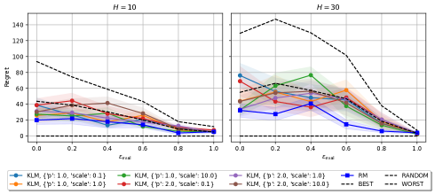
Figure 1: The horizontal axis indicates the exploration parameter $\epsilon_{\rm eval}$ of the evaluation policy and the vertical axis indicates the excess mean absolute error relative to the best possible choice.

6 Related Work

Zhang and Jiang, (2021) proposed BVFT-PE to solve the hyperparameter selection problem for OPE and gave an upper bound on $\|\hat{Q}-Q^{\pi}\|_{2}$, which can be translated to the OPE error bound via Proposition 1. In comparison, the scope of BVFT-PE is broader than any of the four methods as it is applicable to any Q-function-estimating OPE algorithms. Another major difference is in the theoretical assumption; BVFT-PE relies on assumptions much stronger than Assumption 1. Also, BVFT-PE is not completely hyperparameter-free in terms of the error bound (Theorem 4, Zhang and Jiang, (2021)), relying on the oracle choice of $\epsilon_{\rm dct}$. Another closely related line of research is the loss-minimization formulation of OPE (Baird,, 1995; Feng et al.,, 2019; Dai et al.,, 2018), in which OPE is formulated as ordinary optimization problems with objective functions. The objective functions are readily usable as hyperparameter selection criteria, but there have been no study applying them to minimize the OPE error with theoretical guarantee. Moreover, these objective functions are either inconsistent (unable to select the true operator $B_{\pi}$, e.g., Baird, (1995)) or hyperparameter-dependent by themselves (e.g., Feng et al., (2019); Dai et al., (2018)).

At the bottom of Table 1, we translate these results in a comparative form. Note that RM and RM-FP are the most distribution-mismatch tolerant and the only completely hyperparameter-free methods there. In terms of the misspecification tolerance, KLM and KLM-FP (which is equivalent to $\overline{\hbox{MetaFQE}}$ + Feng et al., (2019)) are the best.

7 Conclusion

We have presented hyperparameter selection methods of FQE and discussed their properties. In particular, RM and RM-FP are the first hyperparameter selection algorithms for FQE with hyperparameter-free error guarantee. We have also confirmed in a toy example that empirical results match the theoretical prediction based on the error guarantee. The major limitation of our analysis is that it is only applicable to FQE-like algorithms.

Possible future directions include extensions of the KLM methods: Theoretical justification on a specific kernel choice and more time-efficient algorithms reducing the factor of $n^{2}$.

Table 2: Comparison of time complexity.

RM	KLM	RM-FP	KLM-FP
$\mathcal{O}(HK^{2}n)$	$\mathcal{O}(HKn^{2})$	$\mathcal{O}(Kn^{5/4}+K^{2}n)$	$\mathcal{O}(Kn^{2})$

Input: Data $\mathcal{D}$, policy $\pi$, operators $\mathcal{X}\coloneqq\left\{X_{k}\right\}_{k=1}^{K}$

Output: Action-value estimate $\hat{Q}$

1 for $k=1,...,K$ do

       ${\rm Reg}_{k}\leftarrow\mathrm{\overline{Regret}}_{\mathcal{D},\pi}(X_{k};\mathcal{X})$ ;

        // (6)

2      

3$\hat{k}\leftarrow\mathop{\mathrm{argmin}}_{1\leq k\leq K}{\rm Reg}_{k}$;

4 return $\texttt{MetaFQE}(X_{\hat{k}})$;

Algorithm 3 FQE with Regret Minimization (FQE-RM)

Input: Data $\mathcal{D}$, policy $\pi$, operator candidates $\mathcal{X}=\{X_{k}\}_{k=1}^{K}$, kernel $\kappa$

Output: Action-value estimate $\hat{Q}$

1 for $k=1,...,K$ do

       ${\rm KL}_{k}\leftarrow\bar{\mathcal{L}}_{\kappa,\mathcal{D},\pi}(X_{k})$ ;

        // (8)

2      

3$\hat{k}\leftarrow\mathop{\mathrm{argmin}}_{1\leq k\leq K}{\rm KL}_{k}$;

4 return $\texttt{MetaFQE}(X_{\hat{k}})$;

Algorithm 4 FQE with Kernel Loss Minimization (FQE-KLM)

Appendix A Details on Experiments

In both settings, we set $\gamma=1$. The expert policies are trained via online reinforcement learning with the soft actor-critic algorithm (Haarnoja et al.,, 2018) so that they attain sufficiently large policy values, where the implementation is given by d3rlpy (Seno and Imai,, 2021). The actual reward of the experts are reported in Table 3. The candidate set $\mathcal{X}$ consists of the FQE operators of GBDTRegressor from LightGBM with different number of trees, ${\tt n\_estimators}\in\{2^{0},2^{1},...,2^{7}\}$, where the regressors are fitted on i.i.d. sample of $n=480$ and the other parameters are set to default. KLM is run with the exponential-type kernel

$$\kappa(u,\tilde{u})=\exp\left\{-\left|u-\tilde{u}\right|_{p}/\sigma\right\},$$ (10)

where $\left|\cdot\right|_{p}$ is the $\ell^{p}$-norm of vectors and $\sigma$ is the scale parameter. We employed six different kernels with the combination of $p\in\left\{1,2\right\}$ and $\sigma\in\left\{10^{-1},10^{0},10^{1}\right\}$. Moreover, before fed into the kernels or the regressors, the data $(\tilde{s}_{i},\tilde{a}_{i})$ are normalized so that each feature dimension has zero mean and unit variance.

The lines in Figure 1 indicates the excess absolute error, $|\Delta J(\hat{Q})|-\min_{X\in\mathcal{X}}|\Delta J(Q^{X})|$, averaged over 10 independent runs. The shaded areas show the estimated standard deviation of the average.

Table 3: The true policy values of the experts (standard deviation).

$H$	10	30
$J(\pi_{\rm expert})$	211.187 (1.146)	426.978 (0.849)

Appendix B Proofs

B.1 Proofs for Finite Horizon

B.1.1 Proof of Proposition 1

First, we show a useful lemma that characterizes the relationship of the OPE error $\Delta J(Q^{X})$ and the operator error $\Delta X$. It can be seen as a generalization of the telescoping lemma of model-based RL (Lemma 4.3 of Luo et al., (2019), Lemma 4.1 of Yu et al., (2020)). As opposed to these results, Lemma 9 allows the approximate operator $X$ to be those that admit no model-based interpretation.

Lemma 9 (Error identity)

For all $X\in\Omega$,

$$\Delta J(Q^{X}) =\sum_{h=1}^{H}\gamma^{h-1}\mathbb{E}^{\pi}\left[(\Delta XQ^{X}_{H-h})(s_{h},a_{h})\right].$$

Proof  Let $\bar{r}(s,a)\coloneqq\mathbb{E}[R(s,a)]$ and let $P_{\pi}$ be the state-transition operator such that $(P_{\pi}f)(s,a)=\mathbb{E}[f(s^{\prime},\pi(s^{\prime}))|s^{\prime}\sim T(s,a)]$ for $f:{\mathcal{S}}\times\mathcal{A}\to\mathbb{R}$. Then, we have $B_{\pi}f=\bar{r}+\gamma P_{\pi}f$ for all $f:{\mathcal{S}}\times\mathcal{A}\to\mathbb{R}$ and therefore

$$Q^{\pi} =B_{\pi}^{H}0=\sum_{h=1}^{H}\left(\gamma P_{\pi}\right)^{h-1}\bar{r}$$

by the linearity of $P_{\pi}$. Since $P_{\pi}$ is linear, we can telescope the sum to get

$$Q^{\pi} =Q^{X}_{H}-Q^{X}_{0}+\sum_{h=1}^{H}\left(\gamma P_{\pi}\right)^{h-1}\left\{\bar{r}+\gamma P_{\pi}Q^{X}_{H-h}-Q^{X}_{H-h+1}\right\}.$$

Note that $\bar{r}+\gamma P_{\pi}Q^{X}_{H-h}-Q^{X}_{H-h+1}=-\Delta XQ^{X}_{H-h}$. Since we have $Q^{X}_{0}=0$ and $Q^{X}_{H}=Q^{X}$ by definition, we also get

$$Q^{X}-Q^{\pi} =\sum_{h=1}^{H}\left(\gamma P_{\pi}\right)^{h-1}\Delta XQ^{X}_{H-h}.$$

Taking expectation of both sides as in the definition of $J(Q^{\pi})$, we get

$$\Delta\hat{J}(Q^{X}) =\sum_{h=1}^{H}\gamma^{h-1}\mathbb{E}\left[(P_{\pi}^{h-1}\Delta XQ^{X}_{H-h})(s_{1},a_{1})\right].$$

Since $\mathbb{E}[(P_{\pi}f)(s_{h},a_{h})]=\mathbb{E}[f(s_{h+1},a_{h+1})]$ for $h\geq 1$ and $f:{\mathcal{S}}\times\mathcal{A}\to\mathbb{R}$, we obtain the desired result by induction.  

Now we are ready to prove Proposition 1.

Proof  Let $\varphi_{h}(x)\coloneqq\inf_{\left\|f\right\|_{\mathcal{F}}\leq x}\left\|w_{h}-f\right\|_{1}$. Now, by Lemma 9, we have

$$\left|\Delta J(Q^{X})\right| =\left|\sum_{h=1}^{H}\gamma^{h-1}\mathbb{E}_{(s,a)\sim\mu}\left[w_{h}(s,a)\cdot(\Delta XQ^{X}_{H-h})(s,a)\right]\right|$$

$$=\sum_{h=1}^{H}\gamma^{h-1}\left|\mathbb{E}_{(s,a)\sim\mu}\left[w_{h}(s,a)\cdot(\Delta XQ^{X}_{H-h})(s,a)\right]\right|.$$

Fix any $x>0$ and $f\in\mathcal{F}$ satisfying $\left\|f\right\|_{\mathcal{F}}\leq x$. Each summand is bounded as

$$\left|\mathbb{E}_{(s,a)\sim\mu}\left[w_{h}(s,a)\cdot(\Delta XQ^{X}_{H-h})(s,a)\right]\right|$$

$$=\left|\mathbb{E}_{(s,a)\sim\mu}\left[(w_{h}-f+f)(s,a)\cdot(\Delta XQ^{X}_{H-h})(s,a)\right]\right|$$

$$\leq\left\|\Delta XQ^{X}_{H-h}\right\|_{\infty}\left\|w_{h}-f\right\|_{1}+\left|\mathbb{E}_{(s,a)\sim\mu}\left[f(s,a)\cdot(\Delta XQ^{X}_{H-h})(s,a)\right]\right| (\text{H\"{o}lder's inequality})$$

$$\leq C\left\|w_{h}-f\right\|_{1}+x\left\|\Delta XQ^{X}_{H-h}\right\|_{\mathcal{F}^{*}}.$$

The last inequality is owing to the boundedness of the range of $X\in\Omega$. Taking the infimum over $f$, we get

$$\left|\mathbb{E}_{(s,a)\sim\mu}\left[w_{h}(s,a)\cdot(\Delta XQ^{X}_{H-h})(s,a)\right]\right| \leq C\varphi_{h}(x)+x\left\|\Delta XQ^{X}_{H-h}\right\|_{\mathcal{F}^{*}}$$

for all $x>0$. Putting it back to the summation, we get

$$\left|\Delta J(Q^{X})\right| \leq\sum_{h=1}^{H}\gamma^{h-1}\left\{C\varphi_{h}(x)+x\left\|\Delta XQ^{X}_{H-h}\right\|_{\mathcal{F}^{*}}\right\}$$

$$=C\sum_{h=1}^{H}\gamma^{h-1}\varphi_{h}(x)+x\sum_{h=1}^{H}\gamma^{h-1}\left\|\Delta XQ^{X}_{H-h}\right\|_{\mathcal{F}^{*}}.$$

We get the desired result by taking the infimum over $x>0$ and defining

$$\varphi_{\mathcal{F}}(y) \coloneqq C\inf_{x>0}\left\{\sum_{h=1}^{H}\gamma^{h-1}\varphi_{h}(x)+xy\right\}.$$

The nonnegativity and monotonicity of $\varphi_{\mathcal{F}}(y)$, $y\geq 0$, are trivial from the definition. Note that it is concave also by the definition, which implies the continuity except on the boundary $y=0$. Therefore, it suffices to show the boundary condition $\lim_{y\downarrow 0}\varphi_{\mathcal{F}}(y)=\varphi_{\mathcal{F}}(0)=0$. In fact, it is a direct consequence of $\varphi_{h}(x)\to 0$ as $x\to\infty$, $1\leq h\leq H$, which is the case since $\mathcal{F}$ is dense in $L^{1}(\mu)$ and $w_{h}\in L^{1}(\mu)$ by the assumptions.

 

B.1.2 Proof of Proposition 2

Proof  Let $\tilde{z}_{i}(X,f)\coloneqq\bar{r}_{i}+\gamma f(\tilde{s}^{\prime}_{i},\pi(\tilde{s}^{\prime}_{i}))-(Xf)(\tilde{s}_{i},\tilde{a}_{i})$, $m_{i}(X,f)\coloneqq\mathbb{E}\left[\tilde{z}_{i}(X,f)\middle|\tilde{s}_{i},\tilde{a}_{i}\right]$, and $v_{i}(f)\coloneqq\mathbb{E}\left[\{\bar{r}_{i}+\gamma f(\tilde{s}^{\prime}_{i},\pi(\tilde{s}^{\prime}_{i}))\}^{2}\middle|\tilde{s}_{i},\tilde{a}_{i}\right]$, $1\leq i\leq n$. Observe that $m_{i}^{2}(X,f)=-(\Delta Xf)(\tilde{s}_{i},\tilde{a}_{i})$ and therefore $\mathbb{E}[m_{i}^{2}(X,f)]=\left\|\Delta Xf\right\|_{2}^{2}$ for $1\leq i\leq n$. Thus,

$$\mathbb{E}\left[\mathcal{L}_{\mathcal{D},\pi}(X;f)\right] =\mathbb{E}\left[\frac{1}{n}\sum_{i=1}^{n}\tilde{z}_{i}^{2}(X,f)\right]$$

$$=\mathbb{E}\left[\tilde{z}_{1}^{2}(X,f)\right]$$

$$=\mathbb{E}\left[m_{1}^{2}(X,f)\right]+\mathbb{E}\left\{\tilde{z}_{1}(X,f)-m_{1}(X,f)\right\}^{2}$$

$$=\left\|\Delta Xf\right\|_{2}^{2}+\mathbb{E}\left[v_{1}^{2}(f)\right].$$

In particular, we have

$$\mathbb{E}\left[\mathcal{L}_{\mathcal{D},\pi}(B^{\pi};f)\right] =\mathbb{E}\left[v_{1}^{2}(f)\right]$$

since $\Delta X=0$ if $X=B_{\pi}$. Taking the difference of the above equations, we get the desired result.  

B.1.3 Proof of Proposition 3

First, we show the following lemma showing the regret is a good estimate of $\|\Delta Xf\|_{2}$ if the set $\mathcal{X}$ well approximates the true operator $B_{\pi}$ in a collective sense.

Lemma 10

Let $\delta\in(0,1)$, $f:{\mathcal{S}}\times\mathcal{A}\to[0,C]$, $\mathcal{X}\subset\Omega$ and $X\in\mathcal{X}$. Then, we have

$$\left|\left\|\Delta Xf\right\|_{2}-\sqrt{\mathrm{Regret}_{\mathcal{D},\pi}(X;\mathcal{X},f)}\right| \leq\min_{A\in\mathcal{X}}\left\|\Delta A\right\|_{2}+C\left(\frac{2\ln(2\left|\mathcal{X}\right|/\delta)}{n}\right)^{\frac{1}{4}}$$

with probability $1-\delta$.

Proof  Let $f:{\mathcal{S}}\times\mathcal{A}\to[0,C]$. With Proposition 2, observe

$$\left|\left\|\Delta Xf\right\|_{2}^{2}-\mathrm{Regret}_{\mathcal{D},\pi}(X;\mathcal{X},f)\right| \leq\underbrace{\left|\mathbb{E}\left[\mathcal{L}_{\mathcal{D},\pi}(X;f)\right]-\mathcal{L}_{\mathcal{D},\pi}(X;f)\right|}_{\text{(A)}}+$$

$$\quad\underbrace{\left|\min_{A\in\mathcal{X}}\mathcal{L}_{\mathcal{D},\pi}(X;f)-\min_{A\in\mathcal{X}}\mathbb{E}\left[\mathcal{L}_{\mathcal{D},\pi}(A;f)\right]\right|}_{\text{(B)}}+$$

$$\quad\underbrace{\left|\min_{A\in\mathcal{X}}\mathbb{E}\left[\mathcal{L}_{\mathcal{D},\pi}(A;f)-\mathcal{L}_{\mathcal{D},\pi}(B_{\pi};f)\right]\right|}_{\text{(C)}}.$$

By Hoeffding’s inequality, we have

$$\left|\mathbb{E}\left[\mathcal{L}_{\mathcal{D},\pi}(X;f)\right]-\mathcal{L}_{\mathcal{D},\pi}(X;f)\right|\leq C^{2}\sqrt{\frac{\ln(2/\delta)}{2n}}$$

with probability $1-\delta$ for $X\in\Omega$. Thus, by taking union bound with $X\in\mathcal{X}$,

$$\text{(A)}\leq C^{2}\sqrt{\frac{\ln(2K/\delta)}{2n}}, \text{(B)}\leq C^{2}\sqrt{\frac{\ln(2K/\delta)}{2n}},$$

with probability $1-\delta$, where $K\coloneqq\left|\mathcal{X}\right|$. As for (C), we have

$$\text{(C)}=\min_{A\in\mathcal{X}}\left\|\Delta Af\right\|_{2}^{2}\leq\min_{A\in\mathcal{X}}\left\|\Delta A\right\|_{2}^{2}.$$

by Proposition 2. Combining the upper bounds on (A), (B) and (C), we get

$$\left|\left\|\Delta Xf\right\|_{2}^{2}-\mathrm{Regret}_{\mathcal{D},\pi}(X;\mathcal{X},f)\right| \leq\min_{A\in\mathcal{X}}\left\|\Delta A\right\|_{2}^{2}+2C^{2}\sqrt{\frac{\ln(2\left|\mathcal{X}\right|/\delta)}{2n}}$$

with probability $1-\delta$. The desired result is obtained by the fact $|\sqrt{a}-\sqrt{b}|\leq\sqrt{|a-b|}$, $a,b\geq 0$.  

Lemma 10 immediately yields the following corollary.

Corollary 11

Let $\delta\in(0,1)$ and $\mathcal{X}\subset\Omega$. Then, we have

$$\left|\tilde{\mathcal{C}}_{L^{2}(\mu)}(X)-\mathrm{\overline{Regret}}_{\mathcal{D},\pi}(X;\mathcal{X})\right| \leq\min_{A\in\mathcal{X}}\left\|\Delta A\right\|_{2}+C\left(\frac{2\ln(2H\left|\mathcal{X}\right|^{2}/\delta)}{n}\right)^{1/4}$$

with probability $1-\delta$ for all $X\in\mathcal{X}$ simultaneously.

Proof  Applying Lemma 10 with the union bound over $X\in\mathcal{X}$ and $f\in\{Q^{X}_{h-1}\}_{h=1}^{H}$, we get the desired result, i.e.,

$$\left|\tilde{\mathcal{C}}_{L^{2}(\mu)}(X)-\mathrm{\overline{Regret}}_{\mathcal{D},\pi}(X;\mathcal{X})\right| \leq\frac{1}{C}\sum_{h=1}^{H}\gamma^{H-h}\left|\left\|\Delta XQ^{X}_{h-1}\right\|_{2}-\sqrt{\mathrm{Regret}_{\mathcal{D},\pi}(X;\mathcal{X},Q^{X}_{h-1})}\right|$$

$$\leq\min_{A\in\mathcal{X}}\left\|\Delta A\right\|_{2}+C\left(\frac{2\ln(2K^{2}H/\delta)}{n}\right)^{\frac{1}{4}}$$

for all $X\in\mathcal{X}$ with probability $1-\delta$.  

Now we are ready to prove Proposition 3.

Proof  By Corollary 11,

$$\tilde{\mathcal{C}}_{L^{2}(\mu)}({\hat{X}_{\rm RM}})-\min_{X\in\mathcal{X}}\tilde{\mathcal{C}}_{L^{2}(\mu)}(X)$$

$$\leq\mathrm{\overline{Regret}}_{\mathcal{D},\pi}({\hat{X}_{\rm RM}};\mathcal{X})-\min_{X\in\mathcal{X}}\mathrm{\overline{Regret}}_{\mathcal{D},\pi}(X;\mathcal{X})+2\left\{\min_{X\in\mathcal{X}}\left\|\Delta X\right\|_{2}+C\left(\frac{2\ln(2H\left|\mathcal{X}\right|^{2}/\delta)}{n}\right)^{1/4}\right\}$$

$$=2\left\{\min_{X\in\mathcal{X}}\left\|\Delta X\right\|_{2}+C\left(\frac{2\ln(2H\left|\mathcal{X}\right|^{2}/\delta)}{n}\right)^{1/4}\right\},$$

where the last equality is owing to the definition of ${\hat{X}_{\rm RM}}$. Since $\tilde{\mathcal{C}}_{L^{2}(\mu)}(X)\leq\left\|\Delta X\right\|_{2}$ for $X\in\Omega$, we have

$$\min_{X\in\mathcal{X}}\tilde{\mathcal{C}}_{L^{2}(\mu)}(X)\leq\min_{X\in\mathcal{X}}\left\|\Delta X\right\|_{2}.$$

Combining the above, we get

$$\tilde{\mathcal{C}}_{L^{2}(\mu)}({\hat{X}_{\rm RM}}) \leq 3\min_{X\in\mathcal{X}}\left\|\Delta X\right\|_{2}+2C\left(\frac{2\ln(2H\left|\mathcal{X}\right|^{2}/\delta)}{n}\right)^{1/4}$$

with probability $1-\delta$. Applying $\varphi_{L^{2}(\mu)}(\cdot)$ on both sides, we further get

$$\left|\Delta J(Q^{{\hat{X}_{\rm RM}}})\right|$$

$$\leq\varphi_{L^{2}(\mu)}(\tilde{\mathcal{C}}_{L^{2}(\mu)}({\hat{X}_{\rm RM}}))$$

$$\leq\varphi_{L^{2}(\mu)}\left(3\min_{X\in\mathcal{X}}\left\|\Delta X\right\|_{2}+2C\left(\frac{2\ln(2H\left|\mathcal{X}\right|^{2}/\delta)}{n}\right)^{1/4}\right)$$

$$\leq\min_{X\in\mathcal{X}}\mathcal{C}_{2}(X)+\varphi_{L^{2}(\mu)}\left(2C\left(\frac{2\ln(2H\left|\mathcal{X}\right|^{2}/\delta)}{n}\right)^{1/4}\right)$$

where the last inequality follows from the monotonicity and the concavity of $\varphi_{L^{2}(\mu)}$. The desired result follows from $\varphi_{\mathcal{F}}(y)\leq C\max_{1\leq h\leq H}\left\|w_{h}\right\|_{\mathcal{F}}y$.  

B.1.4 Proof of Proposition 4

Proof  It suffices to show the first identity. By Mercer’s theorem, there exist a orthonormal basis $\{e_{j}\}_{j=1}^{\infty}$ of $L^{2}(\mu)$ and a sequence of positive numbers $\{\sigma_{j}\}_{j=1}^{\infty}$ such that

$$\kappa(u,\tilde{u})=\sum_{j=1}^{\infty}\sigma_{j}e_{j}(u)e_{j}(\tilde{u}),\quad u,\tilde{u}\in{\mathcal{S}}\times\mathcal{A},$$ (11)

where the convergence is uniform. Observe that any $f\in\mathcal{F}_{\kappa}$ is decomposed as

$$f(u) =\sum_{m=1}^{\infty}\alpha_{m}\kappa(u,u_{m}),\quad u\in{\mathcal{S}}\times\mathcal{A},$$

for some $\alpha_{m}\in\mathbb{R}$ and $u_{m}\in{\mathcal{S}}\times\mathcal{A}$ ($m=1,2,...$), which implies by (11)

$$f(u) =\sum_{j=1}^{\infty}\beta_{j}e_{j}(u),$$

where $\beta_{j}\coloneqq\sigma_{j}\sum_{m=1}^{\infty}\alpha_{m}e_{j}(u_{m})$. The RKHS norm is accordingly decomposed

$$\left\|f\right\|_{\mathcal{F}_{\kappa}}^{2} =\left\langle f,\;f\right\rangle_{\mathcal{F}_{\kappa}}$$

$$=\sum_{m=1}^{\infty}\sum_{\tilde{m}=1}^{\infty}\alpha_{m}\alpha_{\tilde{m}}\kappa(u_{m},u_{\tilde{m}})$$

$$=\sum_{m=1}^{\infty}\sum_{\tilde{m}=1}^{\infty}\alpha_{m}\alpha_{\tilde{m}}\sum_{j=1}^{\infty}\sigma_{j}e_{j}(u_{m})e_{j}(u_{\tilde{m}})$$

$$=\sum_{j=1}^{\infty}\sigma_{j}\left(\sum_{m=1}^{\infty}\alpha_{m}e_{j}(u_{m})\right)^{2}$$

$$=\sum_{j=1}^{\infty}\frac{\beta_{j}^{2}}{\sigma_{j}}.$$

Let $\mathcal{B}\coloneqq\{\left\{\beta_{j}\right\}_{j=1}^{\infty}:\sum_{j=1}^{\infty}\beta_{j}^{2}/\sigma_{j}\leq 1\}$ be the unit ball of the coefficients with respect to $\mathcal{F}_{\kappa}$. Thus, the dual norm is written as

$$\left\|g\right\|_{\mathcal{F}_{\kappa}^{*}}^{2} =\left(\sup_{\left\{\beta_{j}\right\}_{j=1}^{\infty}\in\mathcal{B}}\sum_{j=1}^{\infty}\beta_{j}\mathbb{E}\left[e_{j}(u)g(u)\right]\right)^{2}$$

$$=\sum_{j=1}^{\infty}\sigma_{j}\left\{\mathbb{E}_{u\sim\mu}\left[e_{j}(u)g(u)\right]\right\}^{2}$$

$$=\mathop{\mathbb{E}}_{u,\tilde{u}\sim\mu}\left[\sum_{j=1}^{\infty}\sigma_{j}e_{j}(u)e_{j}(\tilde{u})g(u)g(\tilde{u})\right]$$

$$=\mathop{\mathbb{E}}_{u,\tilde{u}\sim\mu}\left[\kappa(u,\tilde{u})g(u)g(\tilde{u})\right].$$

 

B.1.5 Proof of Proposition 5

First, we introduce the concentration result of the kernel Bellman loss, originally shown by Feng et al., (2020).

Lemma 12

For any $f:{\mathcal{S}}\times\mathcal{A}\to[0,C]$,

$$\left|\left\|\Delta Xf\right\|_{\mathcal{F}_{\kappa}^{*}}-\sqrt{\mathcal{L}_{\kappa,\mathcal{D},\pi}(X;f)}\right|\leq C\left(\frac{4(1\vee\ln 2/\delta)}{n}\right)^{\frac{1}{4}},$$

where $a\vee b\coloneqq\max\left\{a,b\right\}$.

Proof  Proposition 3.1 of Feng et al., (2020) shows

$$\left|\mathcal{L}_{\kappa,\mathcal{D},\pi}(X;f)-\left\|\Delta Xf\right\|_{\mathcal{F}_{\kappa}^{*}}^{2}\right|\leq 2C^{2}\sqrt{\frac{1\vee\ln 2/\delta}{n}},$$

which, together with the concavity of $x\mapsto\sqrt{x}$, implies the desired result.  

Now we are ready for the proof.

Proof  Taking the union bound with Lemma 12, we have, with probability $1-\delta$,

$$\left|\bar{\mathcal{L}}_{\kappa,\mathcal{D},\pi}(X)-\tilde{\mathcal{C}}_{\mathcal{F}_{\kappa}}(X)\right|\leq C\left(\frac{4(1\vee\ln(2H\left|\mathcal{X}\right|/\delta))}{n}\right)^{1/4}$$

for simultaneously all $X\in\mathcal{X}$, which implies

$$\tilde{\mathcal{C}}_{\mathcal{F}_{\kappa}}(\hat{X}_{\mathrm{KLM}(\kappa)})-\max_{X\in\mathcal{X}}\tilde{\mathcal{C}}_{\mathcal{F}_{\kappa}}(X) \leq 2C\left(\frac{4(1\vee\ln(2H\left|\mathcal{X}\right|/\delta))}{n}\right)^{1/4}.$$

Therefore, Proposition 1 yields

$$\mathrm{Subopt}(\hat{X}_{\mathrm{KLM}(\kappa)};\mathcal{X},\mathcal{C}_{\kappa}) =\max\left\{0,\,\left|\Delta J(Q^{\hat{X}_{\mathrm{KLM}(\kappa)}})\right|-\min_{X\in\mathcal{X}}\mathcal{C}(X)\right\}$$

$$\leq\max\left\{0,\,\mathcal{C}_{\kappa}(\hat{X}_{\mathrm{KLM}(\kappa)})-\min_{X\in\mathcal{X}}\mathcal{C}_{\kappa}(X)\right\}$$

$$\leq\varphi_{\mathcal{F}_{\kappa}}\left(2C\left(\frac{4\ln(1\vee 2H\left|\mathcal{X}\right|/\delta)}{n}\right)^{1/4}\right),$$

which, together with $\varphi_{\mathcal{F}}(y)\leq C\max_{1\leq h\leq H}\left\|w_{h}\right\|_{\mathcal{F}}y$, implies the desired result.  

B.2 Proofs for Infinite Horizon

Let us first introduce some useful lemmas.

Lemma 13 (Error identity, fixed-point form)

Suppose $H=\infty$ and $\gamma<1$. Then,

$$\Delta J(Q) =C\mathbb{E}_{(s,a)\sim\nu}\left[(Q-B_{\pi}Q)(s,a)\right]$$

for all $Q:{\mathcal{S}}\times\mathcal{A}\to\mathbb{R}$.

Proof  Fix $Q:{\mathcal{S}}\times\mathcal{A}\to\mathbb{R}$. Take $X\in\Omega$ such that $Xf=Q$ for all $f:{\mathcal{S}}\times\mathcal{A}\to[0,C]$. Then, applying Lemma 9 to $X$ and taking the limit of $H\to\infty$ yields the desired result.  

Lemma 14 (Master error bound, fixed-point form)

Suppose $H=\infty$ and $\gamma<1$. Let $\mathcal{F}\subset L^{1}(\mu)$ be a Banach space. Then, under Assumption 1, there exists a function $\varphi_{\mathcal{F}}:\mathbb{R}_{\geq 0}\to\mathbb{R}_{\geq 0}$ such that $\forall y\geq 0$, $\varphi_{\mathcal{F}}(y)\leq C\left\|w\right\|_{\mathcal{F}}y$ and

$$\left|\Delta J(Q)\right| \leq\varphi_{\mathcal{F}}\left(\left\|Q-B_{\pi}Q\right\|_{\mathcal{F}^{*}}\right)$$ (12)

for all $Q:{\mathcal{S}}\times\mathcal{A}\to\mathbb{R}$. Moreover, if $\mathcal{F}$ is dense in $L^{1}(\mu)$, $\varphi_{\mathcal{F}}$ is a link function.

Proof  It is proved similarly as Proposition 1. The difference is to make sure the existence of $\varphi_{\mathcal{F}}$ since the limit of the link functions of the finite horizon case may not exist. Let $\bar{\varphi}(x)\coloneqq C\inf_{\left\|f\right\|_{\mathcal{F}}\leq x}\left\|w-f\right\|_{1}$. Now, by Proposition 13, we have

$$\left|\Delta J(Q)\right| =C\left|\mathbb{E}_{(s,a)\sim\mu}\left[w(s,a)\cdot(Q-B_{\pi}Q)(s,a)\right]\right|$$

$$=C\left|\mathbb{E}_{(s,a)\sim\mu}\left[(w-f+f)(s,a)\cdot(Q-B_{\pi}Q)(s,a)\right]\right|$$

$$\leq C\left\|w-f\right\|_{1}\left\|Q-B_{\pi}Q\right\|_{\infty}+C\left|\mathbb{E}_{(s,a)\sim\mu}\left[f(s,a)\cdot(Q-B_{\pi}Q)(s,a)\right]\right| (\text{H\"{o}lder's inequality})$$

$$\leq C^{2}\left\|w-f\right\|_{1}+Cx\left\|Q-B_{\pi}Q\right\|_{\mathcal{F}^{*}}$$

for all $f\in\mathcal{F}$ satisfying $\left\|f\right\|_{\mathcal{F}}\leq x$. The last inequality is owing to the boundedness of the range of $X\in\Omega$. Taking the infimum over $f$, we get

$$\left|\Delta J(Q)\right| \leq C\left\{\bar{\varphi}(x)+x\left\|Q-B_{\pi}Q\right\|_{\mathcal{F}^{*}}\right\}$$

for all $x>0$. We get the desired result by further taking the infimum over $x>0$ and defining

$$\varphi_{\mathcal{F}}(y) \coloneqq C\inf_{x>0}\left\{\bar{\varphi}(x)+xy\right\}.$$

That $\varphi_{\mathcal{F}}$ is a link function is proved in the same way as Proposition 1.  

B.2.1 Proof of Proposition 6

Proof  First, suppose we found a fixed point of $X$, i.e., there exists $1\leq h\leq H^{*}$ such that $\bar{Q}^{X}_{H^{*}}=Q^{X}_{h}=Q^{X}_{h+1}$. Then,

$$\left\|\bar{Q}^{X}_{H^{*}}-B_{\pi}\bar{Q}^{X}_{H^{*}}\right\|_{\mathcal{F}^{*}} =\left\|Q^{X}_{h+1}-B_{\pi}Q^{X}_{h}\right\|_{\mathcal{F}^{*}}$$

$$=\left\|\Delta XQ^{X}_{h}\right\|_{\mathcal{F}^{*}}$$

$$\leq\left\|\Delta X\right\|_{\mathcal{F}^{*}},$$

which yields the desired inequality. In the other case, we have $\bar{Q}^{X}_{H^{*}}=\frac{1}{H^{*}}\sum_{h=1}^{H^{*}}Q^{X}_{h}$. Therefore,

$$\left\|\bar{Q}^{X}_{H^{*}}-B_{\pi}\bar{Q}^{X}_{H^{*}}\right\|_{\mathcal{F}^{*}} =\left\|\frac{1}{H^{*}}\sum_{h=1}^{H^{*}}Q^{X}_{h}-B_{\pi}\frac{1}{H^{*}}\sum_{h=1}^{H^{*}}Q^{X}_{h}\right\|_{\mathcal{F}^{*}}$$

$$=\frac{1}{H^{*}}\left\|\sum_{h=1}^{H^{*}}\Delta XQ^{X}_{h}+Q^{X}_{1}-Q^{X}_{H^{*}+1}\right\|_{\mathcal{F}^{*}} (\text{$B_{\pi}$ is affine})$$

$$\leq\left\|\Delta X\right\|_{\mathcal{F}^{*}}+\frac{1}{H^{*}}\left\|Q^{X}_{1}-Q^{X}_{H^{*}+1}\right\|_{\mathcal{F}^{*}}.$$

Now, let $M(\mathcal{F})\coloneqq\sup_{\|f\|_{\mathcal{F}}\leq 1}\|f\|_{1}$, which is finite. Then, for all $g\in\mathcal{F}^{*}$,

$$\left\|g\right\|_{\mathcal{F}^{*}} =\sup_{\left\|f\right\|_{\mathcal{F}}\leq 1}\mathbb{E}_{(s,a)\sim\mu}\left[f(s,a)g(s,a)\right]$$

$$\leq\sup_{\left\|f\right\|_{1}\leq M(\mathcal{F})}\mathbb{E}_{(s,a)\sim\mu}\left[f(s,a)g(s,a)\right]$$

$$=M(\mathcal{F})\sup_{\left\|f\right\|_{1}\leq 1}\mathbb{E}_{(s,a)\sim\mu}\left[f(s,a)g(s,a)\right]$$

$$=M(\mathcal{F})\left\|g\right\|_{\infty}.$$

Combining all the above, we get

$$\left\|\bar{Q}^{X}_{H^{*}}-B_{\pi}\bar{Q}^{X}_{H^{*}}\right\|_{\mathcal{F}^{*}} \leq\left\|\Delta X\right\|_{\mathcal{F}^{*}}+\frac{M(\mathcal{F})}{H^{*}}\left\|Q^{X}_{1}-Q^{X}_{H^{*}+1}\right\|_{\infty}$$

$$\leq\left\|\Delta X\right\|_{\mathcal{F}^{*}}+\frac{C}{H^{*}}M(\mathcal{F}).$$

 

B.2.2 Proof of Proposition 7

Proof  The proof is similar to that of Proposition 3. Let $c(X)\coloneqq\left\|\bar{Q}_{H^{*}}^{X}-B_{\pi}\bar{Q}_{H^{*}}^{X}\right\|_{2}$ and $\rho(X)\coloneqq\sqrt{\mathrm{Regret}^{*}_{\mathcal{D},\pi}(\bar{Q}_{H^{*}}^{X};\mathcal{X})}$. Then, by Lemma 10, we have

$$\left|c(X)-\rho(X)\right|\leq\min_{A\in\mathcal{X}}\left\|\Delta A\right\|_{2}+C\left(\frac{2\ln(2\left|\mathcal{X}\right|^{2}/\delta)}{n}\right)^{\frac{1}{4}}$$

with probability $1-\delta$ simultaneously all $X\in\mathcal{X}$, which implies

$$c({\hat{X}_{\text{\rm RM-FP}}})-\min_{X\in\mathcal{X}}c(X) \leq\rho({\hat{X}_{\text{\rm RM-FP}}})-\min_{X\in\mathcal{X}}\rho(X)+2\min_{X\in\mathcal{X}}\left\|\Delta X\right\|_{2}+2C\left(\frac{2\ln(2\left|\mathcal{X}\right|^{2}/\delta)}{n}\right)^{\frac{1}{4}}$$

$$\leq 2\min_{X\in\mathcal{X}}\left\|\Delta X\right\|_{2}+2C\left(\frac{2\ln(2\left|\mathcal{X}\right|^{2}/\delta)}{n}\right)^{\frac{1}{4}},$$

where the last inequality is owing to the definition of ${\hat{X}_{\text{\rm RM-FP}}}$.

Note that $c(X)\leq\left\|\Delta X\right\|_{2}+\frac{C}{H^{*}}M(L^{2}(\mu))$ by Proposition 6. Since $M(L^{2}(\mu))=1$ (see the proof of Proposition 6 for the definition of $M(\mathcal{F})$) and $H^{*}\geq n^{1/4}$, we have

$$\min_{X\in\mathcal{X}}c(X)\leq\min_{X\in\mathcal{X}}\left\|\Delta X\right\|_{2}+\frac{C}{n^{1/4}}.$$

Combining the above, we get

$$c({\hat{X}_{\text{\rm RM-FP}}}) \leq 3\min_{X\in\mathcal{X}}\left\|\Delta X\right\|_{2}+3C\left(\frac{2\ln(2\left|\mathcal{X}\right|/\delta)}{n}\right)^{1/4}$$

with probability $1-\delta$. Invoking Lemma 14, we further get

$$\left|\Delta J(Q^{{\hat{X}_{\text{\rm RM-FP}}}})\right| \leq\varphi_{L^{2}(\mu)}(c({\hat{X}_{\text{\rm RM-FP}}}))$$

$$\leq\varphi_{L^{2}(\mu)}\left(3\min_{X\in\mathcal{X}}\left\|\Delta X\right\|_{2}+3C\left(\frac{2\ln(2\left|\mathcal{X}\right|/\delta)}{n}\right)^{1/4}\right)$$

$$\leq\min_{X\in\mathcal{X}}\mathcal{C}_{2}(X)+\varphi_{L^{2}(\mu)}\left(3C\left(\frac{2\ln(2\left|\mathcal{X}\right|/\delta)}{n}\right)^{1/4}\right)$$

where the last inequality follows from the monotonicity and the concavity of $\varphi_{L^{2}(\mu)}$. The desired result follows from $\varphi_{\mathcal{F}}(y)\leq C\left\|w\right\|_{\mathcal{F}}y$.  

B.2.3 Proof of Proposition 8

Proof  Let $c(X)\coloneqq\left\|\bar{Q}_{H^{*}}^{X}-B_{\pi}\bar{Q}_{H^{*}}^{X}\right\|_{\mathcal{F}_{\kappa}^{*}}$ and $\rho(X)\coloneqq\sqrt{\mathcal{L}_{\kappa,\mathcal{D},\pi}^{*}(X)}$. Then, by Lemma 12, we have

$$\left|c(X)-\rho(X)\right|\leq C\left(\frac{4(1\vee\ln(2\left|\mathcal{X}\right|/\delta))}{n}\right)^{\frac{1}{4}}$$

with probability $1-\delta$ simultaneously all $X\in\mathcal{X}$, which implies

$$c(\hat{X}_{\text{\rm KLM-FP}(\kappa)})-\min_{X\in\mathcal{X}}c(X) \leq\rho(\hat{X}_{\text{\rm KLM-FP}(\kappa)})-\min_{X\in\mathcal{X}}\rho(X)+2C\left(\frac{4(1\vee\ln(2\left|\mathcal{X}\right|/\delta))}{n}\right)^{\frac{1}{4}}$$

$$\leq 2C\left(\frac{4(1\vee\ln(2\left|\mathcal{X}\right|/\delta))}{n}\right)^{\frac{1}{4}},$$

where the last inequality is owing to the definition of $\hat{X}_{\text{\rm KLM-FP}(\kappa)}$.

Note that $c(X)\leq\left\|\Delta X\right\|_{\mathcal{F}_{\kappa}^{*}}+\frac{C}{n^{1/4}}M(\mathcal{F}_{\kappa})$ by Proposition 6. Note also $M(\mathcal{F}_{\kappa})\leq 1$ since $\kappa$ is normalized (see the proof of Proposition 6 for the definition of $M(\mathcal{F})$). Thus, we have

$$\min_{X\in\mathcal{X}}c(X)\leq\min_{X\in\mathcal{X}}\left\|\Delta X\right\|_{\mathcal{F}_{\kappa}^{*}}+\frac{C}{n^{1/4}},$$

which implies

$$c(\hat{X}_{\text{\rm KLM-FP}(\kappa)}) \leq\min_{X\in\mathcal{X}}\left\|\Delta X\right\|_{\mathcal{F}_{\kappa}^{*}}+3C\left(\frac{4(1\vee\ln(2\left|\mathcal{X}\right|/\delta))}{n}\right)^{\frac{1}{4}}.$$

Finally, the desired result is given by applying Lemma 14 to the LHS.

References

• Baird, (1995) Baird, L. (1995). Residual algorithms: Reinforcement learning with function approximation. In Machine Learning Proceedings 1995, pages 30–37. Elsevier.
• Dai et al., (2018) Dai, B., Shaw, A., Li, L., Xiao, L., He, N., Liu, Z., Chen, J., and Song, L. (2018). Sbeed: Convergent reinforcement learning with nonlinear function approximation. In International Conference on Machine Learning, pages 1125–1134. PMLR.
• Duan et al., (2020) Duan, Y., Jia, Z., and Wang, M. (2020). Minimax-optimal off-policy evaluation with linear function approximation. In International Conference on Machine Learning, pages 2701–2709. PMLR.
• Feng et al., (2019) Feng, Y., Li, L., and Liu, Q. (2019). A kernel loss for solving the bellman equation. arXiv preprint arXiv:1905.10506.
• Feng et al., (2020) Feng, Y., Ren, T., Tang, Z., and Liu, Q. (2020). Accountable off-policy evaluation with kernel bellman statistics. In International Conference on Machine Learning, pages 3102–3111. PMLR.
• Haarnoja et al., (2018) Haarnoja, T., Zhou, A., Abbeel, P., and Levine, S. (2018). Soft actor-critic: Off-policy maximum entropy deep reinforcement learning with a stochastic actor. In International conference on machine learning, pages 1861–1870. PMLR.
• Hubbs et al., (2020) Hubbs, C. D., Perez, H. D., Sarwar, O., Sahinidis, N. V., Grossmann, I. E., and Wassick, J. M. (2020). Or-gym: A reinforcement learning library for operations research problems. arXiv preprint arXiv:2008.06319.
• Le et al., (2019) Le, H., Voloshin, C., and Yue, Y. (2019). Batch policy learning under constraints. In International Conference on Machine Learning, pages 3703–3712. PMLR.
• Levine et al., (2020) Levine, S., Kumar, A., Tucker, G., and Fu, J. (2020). Offline reinforcement learning: Tutorial, review, and perspectives on open problems. arXiv preprint arXiv:2005.01643.
• Luo et al., (2019) Luo, Y., Xu, H., Li, Y., Tian, Y., Darrell, T., and Ma, T. (2019). Algorithmic framework for model-based deep reinforcement learning with theoretical guarantees. In International Conference on Learning Representations.
• Paine et al., (2020) Paine, T. L., Paduraru, C., Michi, A., Gulcehre, C., Zolna, K., Novikov, A., Wang, Z., and de Freitas, N. (2020). Hyperparameter selection for offline reinforcement learning. arXiv preprint arXiv:2007.09055.
• Seno and Imai, (2021) Seno, T. and Imai, M. (2021). d3rlpy: An offline deep reinforcement library. In NeurIPS 2021 Offline Reinforcement Learning Workshop.
• Xie and Jiang, (2021) Xie, T. and Jiang, N. (2021). Batch value-function approximation with only realizability. In International Conference on Machine Learning, pages 11404–11413. PMLR.
• Yu et al., (2020) Yu, T., Thomas, G., Yu, L., Ermon, S., Zou, J. Y., Levine, S., Finn, C., and Ma, T. (2020). Mopo: Model-based offline policy optimization. In Larochelle, H., Ranzato, M., Hadsell, R., Balcan, M. F., and Lin, H., editors, Advances in Neural Information Processing Systems, volume 33, pages 14129–14142. Curran Associates, Inc.
• Zhang and Jiang, (2021) Zhang, S. and Jiang, N. (2021). Towards hyperparameter-free policy selection for offline reinforcement learning. Advances in Neural Information Processing Systems, 34.