Local and Global Convergence of General Burer-Monteiro Tensor Optimizations

Abstract

Tensor optimization is crucial to massive machine learning and signal processing tasks. In this paper, we consider tensor optimization with a convex and well-conditioned objective function and reformulate it into a nonconvex optimization using the Burer-Monteiro type parameterization. We analyze the local convergence of applying vanilla gradient descent to the factored formulation and establish a local regularity condition under mild assumptions. We also provide a linear convergence analysis of the gradient descent algorithm started in a neighborhood of the true tensor factors. Complementary to the local analysis, this work also characterizes the global geometry of the best rank-one tensor approximation problem and demonstrates that for orthogonally decomposable tensors the problem has no spurious local minima and all saddle points are strict except for the one at zero which is a third-order saddle point.

1 Introduction

Tensors, a multi-dimensional generalization of vectors and matrices, provide natural representations for multi-way datasets and find numerous applications in machine learning and signal processing, including video processing (Liu et al. 2012), hyperspectral imaging (Li et al. 2015b; Sun et al. 2020), collaborative filtering (Hou and Qian 2017), latent graphical model learning (Anandkumar, Ge, and Janzamin 2017), independent component analysis (ICA) (Cardoso 1989), dictionary learning (Barak, Kelner, and Steurer 2015), neural networks compression  (Phan et al. 2020; Bai et al. 2021), Gaussian mixture estimation (Sedghi, Janzamin, and Anandkumar 2016), and psychometrics (Smilde, Bro, and Geladi 2005). See (Sidiropoulos et al. 2017) for a review. All these applications involve solving certain optimizations over the space of low-rank tensors:

$$\operatorname*{minimize}_{T} ~{}f(T)~{}~{}\operatorname*{subject\ to\ }~{}{\operatorname{rank}}(T)\leq r.$$ (1)

Here $f(\cdot)$ is a problem dependent objective function with tensor argument and ${\operatorname{rank}}(\cdot)$ calculates the tensor rank. The rank of matrices is well-understood and has many equivalent definitions, such as the dimension of the range space, or the size of largest non-vanishing minor, or the number of nonzero singular values. The latter is also equal to the smallest number of rank-one factors that the matrix can be written as a sum of. The tensor rank, however, has several non-equivalent variants, among which the Tucker rank (Kolda and Bader 2009) and the Canonical Polyadic (CP) rank (Grasedyck, Kressner, and Tobler 2013) are most well-known. The CP tensor rank is a more direct generalization from the matrix case and is precisely equal to the minimal number of terms in a rank-one tensor decomposition. It is also the preferred notion of rank in applications. Unfortunately, while the Tucker rank can be found by performing the higher-order singular value decomposition (HOSVD) of the tensor, the CP rank is NP-hard to compute (Hillar and Lim 2013). Even though some recent works (Yuan and Zhang 2016; Barak and Moitra 2016; Li et al. 2016; Li and Tang 2017; Li et al. 2015a; Tang and Shah 2015) study the convex relaxation methods based on the tensor nuclear norm, which is also NP-hard to compute (Hillar and Lim 2013). Therefore, this work seeks alternative ways to solve the CP rank-constrained tensor optimizations.

General Burer-Monteiro Tensor Optimizations

Throughout this paper, we focus on third-order, symmetric tensors and assume that $f:\mathbb{R}^{n\times n\times n}\rightarrow\mathbb{R}$ is a general convex function and has a unique global minimizer $T^{\star}$ that admits the following (symmetric-)rank-revealing decomposition:

$$T^{\star}=\sum_{p=1}^{r}{c_{p}^{\star}}\widehat{{\boldsymbol{u}}}_{p}\otimes\widehat{{\boldsymbol{u}}}_{p}\otimes\widehat{{\boldsymbol{u}}}_{p}\in\mathbb{R}^{n\times n\times n},$$ (2)

where $\widehat{{\boldsymbol{u}}}_{p}$’s are the normalized tensor factors living on the unit spheres $\mathbb{S}^{n-1}$ and $c_{p}^{\star}$’s are the decomposition coefficients. Without loss of generality, we can always assume $c_{p}^{\star}>0$, since otherwise we can absorb its sign into the normalized tensor factors.

Note that the global optimal tensor in (2) can be rewritten as

$$T^{\star} =\sum_{p=1}^{r}({c_{p}^{\star}}^{1/3}\widehat{{\boldsymbol{u}}}_{p})\otimes({c_{p}^{\star}}^{1/3}\widehat{{\boldsymbol{u}}}_{p})\otimes({c_{p}^{\star}}^{1/3}\widehat{{\boldsymbol{u}}}_{p})$$

$$\doteq U^{\star}\circ U^{\star}\circ U^{\star},$$ (3)

where $U^{\star}\doteq\big{[}{c_{1}^{\star}}^{1/3}\widehat{{\boldsymbol{u}}}_{1}~{}{c_{2}^{\star}}^{1/3}\widehat{{\boldsymbol{u}}}_{2}~{}\cdots~{}{c_{r}^{\star}}^{1/3}\widehat{{\boldsymbol{u}}}_{r}\big{]}$ can be viewed as the “cubic root” of $T^{\star}$. Noting that the “cubic-root” representation (3) has permutation ambiguities, that is, different columnwise permutations of $U^{\star}$ would generate the same tensor in (3): $[{\boldsymbol{u}}_{i_{1}}^{\star}~{}{\boldsymbol{u}}_{i_{2}}^{\star}~{}\cdots~{}{\boldsymbol{u}}_{i_{r}}^{\star}]\circ[{\boldsymbol{u}}_{i_{1}}^{\star}~{}{\boldsymbol{u}}_{i_{2}}^{\star}~{}\cdots~{}{\boldsymbol{u}}_{i_{r}}^{\star}]\circ[{\boldsymbol{u}}_{i_{1}}^{\star}~{}{\boldsymbol{u}}_{i_{2}}^{\star}~{}\cdots~{}{\boldsymbol{u}}_{i_{r}}^{\star}]=U^{\star}\circ U^{\star}\circ U^{\star}$ for any permutation $(i_{1},i_{2},\cdots,i_{r})$ of the index $(1,2,\cdots,r).$ This immediately implies that $U^{\star}$ and its columnwise permutations all give rise to global minimizers of the following reformulation of the optimization (1):

$$\operatorname*{minimize}_{U\in\mathbb{R}^{n\times r}}~{}f(U\circ U\circ U).$$ (4)

Note that this new factorized formulation has explicitly encoded the rank constraint ${\operatorname{rank}}(T)\leq r$ into the factorization representation $T=U\circ U\circ U$. As a result, the rank-constrained optimization problem (1) on tensor variables reduces to the above unconstrained optimization of matrix variables, avoiding dealing with the difficult rank constraint at the price of working with a highly non-convex objective function in $U$. Indeed, while the resulting optimization (4) has no rank constraint, a smaller memory footprint, and is more amenable for applying simple iterative algorithms like gradient descent, the permutational invariance of $f(U\circ U\circ U)$ implies that saddle points abound the optimization landscape among the exponentially many equivalent global minimizers. Unlike the original convex objective $f(T)$ that has an algorithm-friendly landscape where all the stationary points correspond to the global minimizers, the landscape for the resulting nonconvex formulation $f(U\circ U\circ U)$ is not well-understood. On the other hand, simple local search algorithms applied to (4) has exhibited superb empirical performance. As a first step towards understanding of the power of using the factorization method to solve tensor inverse problems, this work will focus on characterizing the local convergence of applying vanilla gradient descent to the general problem (4), as well as the global convergence of a simple variant.

Related Work

Burer-Monteiro Parameterization Method

The idea of transforming the rank-constrained problem into an unconstrained problem using explicit factorization like $T=U\circ U\circ U$ is pioneered by Burer and Monteiro (Burer and Monteiro 2003, 2005) in solving matrix optimization problems with a rank constraint

$$\operatorname*{minimize}_{X\in\mathbb{R}^{n\times n}} ~{}~{}f(X)$$ (5)

$$\operatorname*{subject\ to\ } ~{}~{}{\operatorname{rank}}(X)\leq r~{}\mathrm{and}~{}X\succeq 0$$

To deal with the rank constraint as well as the positive semidefinite constraint, the authors there proposed to firstly factorize a low-rank matrix $X=UU^{\top}$ with $U\in\mathbb{R}^{n\times r}$ and $r$ chosen according to the rank constraint. Consequently, instead of minimizing an objective function $f(X)$ over all symmetric, positive semidefinite matrices of rank at most $r$, one can focus on an unconstrained nonconvex optimization:

$$\operatorname*{minimize}_{U\in\mathbb{R}^{n\times r}}f(UU^{\top}).$$

Inspired by (Burer and Monteiro 2003, 2005), an intensive research effort has been devoted to investigating the theoretical properties of this factorization/parametrization method (Ge, Lee, and Ma 2016; Ge, Jin, and Zheng 2017; Park et al. 2017; Chi, Lu, and Chen 2019; Li, Zhu, and Tang 2018; Zhu et al. 2018, 2021; Li, Zhu, and Tang 2017; Zhu et al. 2019; Li et al. 2020). In particular, by analyzing the landscape of the resulting optimization, many authors have found that various low-rank matrix recovery problems in factored form–despite nonconvexity–enjoy a favorable landscape where all second-order stationary points are global minima.

Tensor Decomposition and Completion

Another line of related work is nonconvex tensor factorization/completion. When the convex objective function $f(T)$ in (1) is the squared Euclidean distance between the tensor variable $T$ and the ground-truth tensor $T^{\star}$, i.e., $f(T)=\|T-T^{\star}\|_{F}^{2}$, the resulting factorized problem (4) reduces to a (symmetric) tensor decomposition problem:

$$\operatorname*{minimize}_{U\in\mathbb{R}^{n\times r}}~{}f(U\circ U\circ U)=\|U\circ U\circ U-T^{\star}\|_{F}^{2}.$$ (6)

Tensor decomposition aims to identify the unknown rank-one factors from available tensor data. This problem is the backbone of several tensor-based machine learning methods, such as independent component analysis (Cardoso 1989) and collaborative filtering (Hou and Qian 2017). Unlike the similarly defined matrix decomposition, which has a closed-form solution given by the singular value decomposition, the tensor decomposition solution generally has no analytic expressions and is NP-hard to compute in the worst case (Hillar and Lim 2013). When the true tensor $T^{\star}$ is a fourth-order symmetric orthogonal tensor, i.e., there is an orthogonal matrix $U^{\star}$ such that $T^{\star}=U^{\star}\circ U^{\star}\circ U^{\star}\circ U^{\star}$, Ge et al. (Ge et al. 2015) designed a new objective function

$$\widetilde{f}(U)\doteq\sum_{i\neq j}\langle T^{\star},{\boldsymbol{u}}_{i}\otimes{\boldsymbol{u}}_{i}\otimes{\boldsymbol{u}}_{j}\otimes{\boldsymbol{u}}_{j}\rangle$$

and showed that, despite its non-convexity, the objective function $\widetilde{f}(U)$ has a benign landscape on the sphere where all the local minima are global minima and all the saddle points have a Hessian with at least one negative eigenvalue. Later, (Qu et al. 2019) relax the orthogonal condition to near-orthogonal condition, resulting to landscape analysis to fourth-order overcomplete tensor decomposition. The work (Ge et al. 2015) has spurred many followups that dedicate on the analysis of the nonconvex optimization landscape of many other problems (Ge, Lee, and Ma 2016; Ge, Jin, and Zheng 2017; Bhojanapalli, Neyshabur, and Srebro 2016; Park et al. 2017; Chi, Lu, and Chen 2019). The techniques developed in (Ge et al. 2015), however, are not directly applicable to solve the original rank-constrained tensor optimization problem (6). In addition, (Ge et al. 2015) mainly considered fourth-order tensor decomposition, which cannot be trivially extended to analyze other odd-order tensor decompositions. More recently, Ge and Ma (Ge and Ma 2017) studied the problem of maximizing

$$\widehat{f}({\boldsymbol{u}})=\langle T,{\boldsymbol{u}}\otimes{\boldsymbol{u}}\otimes{\boldsymbol{u}}\otimes{\boldsymbol{u}}\rangle$$

on the unit sphere and presented a local convergence of applying vanilla gradient descent to the problem. Although this formulation together with iterative rank-1 updates lead to algorithms with convergence guarantees for tensor decomposition, it is not flexible enough to deal with general rank-constrained problem (1). Similar rank-1 updating methods for tensor decomposition have also been investigated in (Anandkumar, Ge, and Janzamin 2017; Anandkumar, Ge, and Janzamin 2015, 2014; Anandkumar et al. 2014).

More recently, (Chi, Lu, and Chen 2019; Cai et al. 2021) apply the factorization formulation to the tensor completion problem and focuses on solving

$$\operatorname*{minimize}_{U\in\mathbb{R}^{n\times r}}~{}\left\|P_{\Omega}\left(U\circ U\circ U-T^{\star}\right)\right\|_{F}^{2},$$ (7)

where $P_{\Omega}$ is the the orthogonal projection of any tensor $T$ onto the subspace indexed by the observation set $\Omega$. (Chi, Lu, and Chen 2019; Cai et al. 2021) proposed a vanilla gradient descent following a rough initialization and proved the vanilla gradient descent could faithfully complete the tensor and retrieve all individual tensor factors within nearly linear time when the rank $r$ does not exceed $O(n^{1/6})$. Compared with these prior state of the arts, our convergence analysis improves the order of rank $r$ and extends the focus to general cost functions.

Main Contributions and Organization

To solve the rank-constrained tensor optimization problem (1), we directly work with the Burer-Monteiro factorized formulation (4) with a general convex function $f(\cdot)$ and focus on solving  (4) using (vanilla) gradient descent

$$U^{+}=U-\eta\nabla_{U}f(U\circ U\circ U),$$ (8)

where $U^{+}$ is the updated version of the current variable $U$, $\eta$ is the stepsize that will be carefully tuned to prevent gradient descent from diverging, and $\nabla_{U}f$ is the gradient of $f(U\circ U\circ U)$ with respect to $U$.

In this work, we show that the factorized tensor minimization problem (4) satisfies the local regularity condition under certain mild assumptions. With this local regularity condition, we further prove a linear convergence of the gradient descent algorithm in a neighborhood of true tensor factors. In particular, we have shown that solving the factored tensor minimization problem (4) with gradient descent (8) is guaranteed to identify the target tensor $T^{\star}$ with high probability if $r=O\big{(}n^{1.25}\big{)}$ and $n$ is sufficiently large. This implies that we can even deal with the scenario where the rank of the target tensor $T^{\star}$ is larger than the individual tensor dimensions, the so called overcomplete regime that are considered challenging to tackle in practice.

Finally, as a complement to the local analysis, we study the global landscape of best rank-1 approximation of a third-order orthogonal tensor and we show that this problem has no spurious local minima and all saddle points are strict saddle points except for the one at zero, which is a third-order saddle point.

Organization

The remainder of this work is organized as follows. In Section 2, we first briefly introduce some basic definitions and concepts used in tensor analysis and then present the local convergence of applying vanilla gradient descent to the tensor minimization problem (4) and provide a linear convergence analysis for the gradient descent algorithm (8). In Section 3, we switch to analyze the global landscape of orthogonal tensor decomposition. Numerical simulations are conducted in Section 4 to further support our theory. Finally, we conclude our work in Section 5.

2 Local Convergence

In this section, we first briefly review some fundamental concepts and definitions in tensor analysis. A tensor with order higher than $3$ can be viewed as a high-dimensional extension of vectors and matrices. In this work, we mainly focus on the third-order symmetric tensors. Any such tensor admits symmetric rank-one decompositions of the following form:

$$T=\sum_{p=1}^{r}{c_{p}}{\boldsymbol{u}}_{p}\otimes{\boldsymbol{u}}_{p}\otimes{\boldsymbol{u}}_{p}\in\mathbb{R}^{n\times n\times n}$$

with $\|{\boldsymbol{u}}_{p}\|_{2}=1$ and $c_{p}>0$, $1\leq p\leq r$. The above decomposition is also called the Canonical Polyadic (CP) decomposition of the tensor $T$ (Hong, Kolda, and Duersch 2020). The minimal number of factors $r$ is defined as the (symmetric) rank of the tensor $T$. Denote $T(i_{1},i_{2},i_{3})$ as the $(i_{1},i_{2},i_{3})$-th entry of a tensor $T$. We define the inner product of any two tensors $X,Y\in\mathbb{R}^{n\times n\times n}$ as $\langle X,Y\rangle\doteq\sum_{i_{1},i_{2},i_{3}=1}^{n}X(i_{1},i_{2},i_{3})Y(i_{1},i_{2},i_{3})$. The induced Frobenius norm of a tensor $T$ is then defined as $\|T\|_{F}\doteq\sqrt{\langle T,T\rangle}.$ For a tensor $T\in\mathbb{R}^{n\times n\times n}$, we denote its unfolding/matricization along the first dimension as $T_{(1)}=[T(:,1,1)~{}T(:,2,1)~{}\cdots~{}T(:,n,n)]\in\mathbb{R}^{n\times n^{2}}.$

We proceed to present the local convergence of applying vanilla gradient descent to the factored tensor minimization problem (4). Before that, we introduce several definitions used throughout the work.

Definition 1.

A function $f:\mathbb{R}^{n\times n\times n}\rightarrow\mathbb{R}$ is $(r,m,M)$-restricted strongly convex and smooth if

$$m\|Y-X\|_{F}\leq\|\nabla f(Y)-\nabla f(X)\|_{F}\leq M\|Y-X\|_{F}$$

holds for any symmetric tensors $X,Y\in\mathbb{R}^{n\times n\times n}$ of rank at most $r$ with some positive constants $m$ and $M$.

For example, $f(T)=\frac{1}{2}\|T-T^{\star}\|_{F}^{2}$ is such a $(r,m,M)$-restricted strongly convex and smooth function for arbitrary $r\in\mathbb{N}$ with $M=m=1$, and its global minimizer is $T=T^{\star}$.

Definition 2.

The distance between two factored matrices $U_{1}$ and $U_{2}$ is defined as

$${\operatorname{dist}}(U_{1},U_{2}) =\min_{{\operatorname{Permutation}}P}\|U_{1}-U_{2}P\|_{F}.$$

Denote

$$P_{U_{1}}=\arg\min_{{\operatorname{Permutation}}P}\|U_{1}-U_{2}P\|_{F}.$$ (9)

Then, we can rewrite the distance between $U_{1}$ and $U_{2}$ as

$${\operatorname{dist}}(U_{1},U_{2})=\|U_{1}-U_{2}P_{U_{1}}\|_{F}.$$ (10)

Define $\gamma\doteq{\operatorname{polylog}}(n)$ that may vary from place to place and $\widehat{U}\doteq\big{[}\widehat{{\boldsymbol{u}}}_{1}~{}\widehat{{\boldsymbol{u}}}_{2}~{}\cdots~{}\widehat{{\boldsymbol{u}}}_{r}\big{]}$. Denote $\underline{c}\doteq\min_{p\in[r]}{c_{p}^{\star}}^{1/3}$, $\bar{c}\doteq\max_{p\in[r]}{c_{p}^{\star}}^{1/3}$, and $\omega=\bar{c}/\underline{c}$. We are ready to introduce the assumptions needed to prove our main theorem as follows.

Assumption 1.

(Incoherence condition). The vector factors $\widehat{{\boldsymbol{u}}}$ in the target tensor $T^{\star}$ satisfy

$$\max_{i\neq j}|\langle\widehat{{\boldsymbol{u}}}_{i},\widehat{{\boldsymbol{u}}}_{j}\rangle|\leq\frac{\gamma}{\sqrt{n}}.$$

Assumption 2.

(Bounded spectrum). The spectral norm of $\widehat{U}$ is bounded above as

$$\|\widehat{U}\|\leq 1+c_{1}\sqrt{\frac{r}{n}}.$$

Assumption 3.

(Isometry of Gram-matrix). The Gram matrix satisfies the following isometry property

$$\|(\widehat{U}^{\top}\widehat{U})\odot({\widehat{U}}^{\top}\widehat{U})-\mathbf{I}_{r}\|\leq\frac{\gamma\sqrt{r}}{n}.$$

where $\odot$ is the Hadamard product.

Assumption 4.

(Warm start). The distance between the current variable $U$ and the matrix factor $U^{\star}$ is bounded with

$${\operatorname{dist}}(U,U^{\star})\leq 0.07\frac{m}{M}\frac{\underline{c}}{\omega^{3}}.$$

We remark that Assumptions 1-3 hold with high probability if the factors $\{\widehat{{\boldsymbol{u}}}_{p}\}_{p=1}^{r}$ are generated independently according to the uniform distribution on the unit sphere (Anandkumar, Ge, and Janzamin 2015, Lemmas 25, 31).

Main Results

We now present our main theorem in the following:

Theorem 1.

Suppose that a $(r,m,M)$-restricted strongly convex and smooth function $f:\mathbb{R}^{n\times n\times n}\rightarrow\mathbb{R}$ has a unique global minimizer at $T^{\star}$, which admits a CP decomposition $T^{\star}=U^{\star}\circ U^{\star}\circ U^{\star}\in\mathbb{R}^{n\times n\times n}$ as given in (3). Then, under Assumptions  1-4 and in addition assuming $r=O\big{(}n^{1.25}\big{)}$, the following local regularity condition holds for sufficiently large $n$:

$$\langle\nabla_{U}f(U\circ U\circ U),U-U^{\star}P_{U}\rangle\geq \frac{1}{2}\eta\|\nabla_{U}f(U\circ U\circ U)\|_{F}^{2}$$ (11)

$$+0.13m\underline{c}^{4}{\operatorname{dist}}(U,U^{\star})^{2},$$

as long as

$$\eta\leq\frac{1}{18\|[\nabla f(T)]_{(1)}\|\cdot\|U\|+9M\|U\|^{4}}.$$ (12)

Here $T=U\circ U\circ U$ and $[\nabla f(T)]_{(1)}$ denotes the matricization of $\nabla f(T)$ along the first dimension.

The local regularity condition further implies linear convergence of the gradient descent algorithm (8) in a neighborhood of the true tensor factors $U^{\star}$ with proper choice of the stepsize, as summarized in the following two corollaries.

Corollary 1 (Linear Convergence with adaptive stepsize).

Under the same assumptions as in Theorem 1, we have the following (adaptive) linear convergence

$${\operatorname{dist}}(U^{+},U^{\star})^{2} \leq(1-0.26\eta m\underline{c}^{4}){\operatorname{dist}}(U,U^{\star})^{2}$$ (13)

$$\doteq\alpha(\eta)\cdot{\operatorname{dist}}(U,U^{\star})^{2}$$

when we run the gradient descent algorithm (8) with the stepsize $\eta$ satisfying (12).

Corollary 2 (Linear Convergence with constant stepsize).

Under the same assumptions as in Theorem 1, except that Assumption 4 is replaced by a good initial condition:

$${\operatorname{dist}}(U^{0},U^{\star})\leq 0.07\frac{m}{M}\frac{\underline{c}}{\omega^{3}},$$ (14)

and the stepsize selection requirement (12) is replaced with the constant stepsize satisfying $\eta_{0}=\frac{1}{21.6M\|U^{0}\|^{4}},$ the sequence $\{U^{t}:t=0,1,2,\cdots\}$ generated by

$$U^{t+1}=U^{t}-\eta_{0}\nabla f(U^{t}\circ U^{t}\circ U^{t}),~{}~{}t=0,1,2,\cdots$$

satisfies

$${\operatorname{dist}}(U^{+},U^{\star})^{2} \leq\alpha(\eta_{0})\cdot{\operatorname{dist}}(U,U^{\star})^{2}$$ (15)

with $\alpha(\eta_{0})\doteq 1-0.26\eta_{0}m\underline{c}^{4}$.

As a consequence, we conclude that solving the factored problem (4) using the gradient descent algorithm (8) with a good initialization is guaranteed to recover the tensor factor matrix $U^{\star}$ with high probability if $r=O\big{(}n^{1.25}\big{)}$. The proof of the above theorem and corollaries can be found in supplementary material.

3 Global Convergence

The local convergence analysis of applying vanilla gradient descent to tensor optimization, though developed for a class of sufficiently general problems, is not completely satisfactory as a good initialization might be difficult to find. Therefore, we are also interested in characterizing the global optimization landscape for these problems. Considering the difficulty of this task, we focus on a special case where the ground-truth third-order tensor admits an orthogonal decomposition and we are interested in finding its best rank-one approximation. We aim to characterize all its critical points and classify them into local minima, strict saddle points, and degenerate saddle points if there is any. We also want to exploit the properties of critical points to design a provable and efficient tensor decomposition algorithm.

Main Results

Consider the best rank-one approximation problem of an orthogonally decomposable tensor:

$$g({\boldsymbol{u}})=\|{\boldsymbol{u}}\otimes{\boldsymbol{u}}\otimes{\boldsymbol{u}}-T^{\star}\|_{F}^{2},$$ (16)

where $T^{\star}=\sum_{i=1}^{r}{\boldsymbol{u}}_{i}^{\star}\otimes{\boldsymbol{u}}_{i}^{\star}\otimes{\boldsymbol{u}}_{i}^{\star}$ and these true tensor factors $\{{\boldsymbol{u}}_{i}^{\star}\}$ are orthogonal to each other. This is a special case of (4) (and (6)). We characterize all possible critical points and their geometric properties in the following theorem:

Theorem 2.

Assume $T^{\star}=\sum_{i=1}^{r}{\boldsymbol{u}}_{i}^{\star}\otimes{\boldsymbol{u}}_{i}^{\star}\otimes{\boldsymbol{u}}_{i}^{\star}$, where $\{{\boldsymbol{u}}_{i}^{\star}\}$ are orthogonal to each other. Then any critical point $\widehat{\boldsymbol{u}}$ of $g({\boldsymbol{u}})$ in (16) takes the form $\widehat{\boldsymbol{u}}=\sum_{i=1}^{r}\lambda_{i}{\boldsymbol{u}}_{i}^{\star}$ for ${\boldsymbol{\lambda}}\doteq[\lambda_{1}~{}\cdots~{}\lambda_{r}]^{\top}\in\mathbb{R}^{r}$ and

1. when $\|{\boldsymbol{\lambda}}\|_{0}=0$, $\widehat{\boldsymbol{u}}=\mathbf{0}$ is a third-order saddle point, i.e., $\nabla^{2}g(\widehat{\boldsymbol{u}})=\mathbf{0}$ and $\nabla^{3}g(\widehat{\boldsymbol{u}})\neq\mathbf{0}$;

2. when $\|{\boldsymbol{\lambda}}\|_{0}=1$, $\widehat{\boldsymbol{u}}={\boldsymbol{u}}_{i}^{\star}$ with $i\in\{1,2,\ldots,r\}$ is a strict local minimum;

3. when $\|{\boldsymbol{\lambda}}\|_{0}\geq 2$, $\widehat{\boldsymbol{u}}$ is a strict saddle point, i.e., $\nabla^{2}g({\boldsymbol{u}})$ has a negative eigenvalue.

Here the $\ell_{0}$ “norm” $\|\cdot\|_{0}$ counts the number of non-zero entries in a vector. Analytic expression for ${\boldsymbol{\lambda}}$ is given in the proof.

Theorem 2 implies that all second-order critical points are the true tensor factors except for zero. Based on this, we develop a provable conceptual tensor decomposition algorithm as follows:

Algorithm 1 Iterative Gradient Descent for Tensor Decomposition

Input: $T^{\star}$
Initialization: $T=T^{\star}$, $\widehat{\boldsymbol{u}}=\mathbf{0}$
Output: Estimated factors $\{{\boldsymbol{u}}_{i}^{\star}\}$

1:  Let $i=0$.

2:  while ${T}\neq\mathbf{0}$ do

3:     if $\widehat{\boldsymbol{u}}\neq\mathbf{0}$ then

4:        $i=i+1.$

5:        ${\boldsymbol{u}}_{i}^{\star}=\widehat{\boldsymbol{u}}$

6:        ${T}\leftarrow{T}-\frac{\langle{T},\widehat{\boldsymbol{u}}\otimes\widehat{\boldsymbol{u}}\otimes\widehat{\boldsymbol{u}}\rangle\widehat{\boldsymbol{u}}\otimes\widehat{\boldsymbol{u}}\otimes\widehat{\boldsymbol{u}}}{\|\widehat{\boldsymbol{u}}\|_{2}^{3}}$

7:     end if

8:     Find a second-order stationary point $\widehat{\boldsymbol{u}}$ of $g({\boldsymbol{u}})=\|{\boldsymbol{u}}\otimes{\boldsymbol{u}}\otimes{\boldsymbol{u}}-{T}\|_{F}^{2}$.

9:  end while

10:  return solution

Corollary 3.

Assume $T^{\star}$ is a third-order orthogonal tensor with the tensor factors $\{{\boldsymbol{u}}_{i}^{\star}\}$. Then with the input $T^{\star}$, Algorithm 1 almost surely recovers all the tensor factors $\{{\boldsymbol{u}}_{i}^{\star}\}$.

Proof of 3.

It mainly follows from the many iterative algorithms can find a second-order stationary point (Lee et al. 2016; Li, Zhu, and Tang 2019; Li et al. 2019; Nesterov and Polyak 2006; Jin et al. 2017). Then by Theorem 2, applying these iterative algorithms to $g({\boldsymbol{u}})$, it converges to either a true tensor factor ${\boldsymbol{u}}_{i}^{\star}$ for $i\in[r]$ or the zero point (as a third-order saddle point is essentially a second-order stationary point). If it converges to a nonzero point, it must be a true tensor factor and we record it. Then we can remove this component by projecting the target tensor $T$ into the orthogonal complement of ${\boldsymbol{u}}_{i}^{\star}$. We repeat this process to the new deflated tensor until we get a zero deflated tensor. That means, we have found all the true factors $\{{\boldsymbol{u}}_{i}^{\star}\}$. ∎

Proof of Theorem 2

Recall that

$$T^{\star}=\sum_{i=1}^{r}{\boldsymbol{u}}_{i}^{\star}\otimes{\boldsymbol{u}}_{i}^{\star}\otimes{\boldsymbol{u}}_{i}^{\star}\doteq\sum_{i=1}^{r}\lambda_{i}\widehat{\boldsymbol{u}}_{i}\otimes\widehat{\boldsymbol{u}}_{i}\otimes\widehat{\boldsymbol{u}}_{i}.$$

Without loss of generality, we can extend the orthonormal set $\{\widehat{\boldsymbol{u}}_{i}\}_{i=1}^{r}$ to $\{\widehat{\boldsymbol{u}}_{i}\}_{i=1}^{n}$ as a full orthonormal basis of $\mathbb{R}^{n}$ and define

$$\lambda_{i}\doteq 0,~{}i\in[r]^{c}\doteq\{r+1,\ldots,n\}.$$

Then, we have $T^{\star}=\sum_{i=1}^{n}\lambda_{i}\widehat{\boldsymbol{u}}_{i}\otimes\widehat{\boldsymbol{u}}_{i}\otimes\widehat{\boldsymbol{u}}_{i}.$ Since $\{\widehat{\boldsymbol{u}}_{i}\}_{i=1}^{n}$ is a full orthonormal basis of $\mathbb{R}^{n}$, $\widehat{U}\doteq[\widehat{\boldsymbol{u}}_{1}\cdots~{}\widehat{\boldsymbol{u}}_{n}]$ is an orthonormal matrix, i.e., $\widehat{U}\widehat{U}^{\top}=\mathbf{I}$. Then the best rank-1 tensor approximation problem is equivalent to

$$g({\boldsymbol{u}}) =\|{\boldsymbol{u}}\otimes{\boldsymbol{u}}\otimes{\boldsymbol{u}}-T^{\star}\|_{F}^{2}$$ (17)

$$=\Big{\|}(\widehat{U}\widehat{U}^{\top}{\boldsymbol{u}})\otimes(\widehat{U}\widehat{U}^{\top}{\boldsymbol{u}})\otimes(\widehat{U}\widehat{U}^{\top}{\boldsymbol{u}})$$

$$~{}~{}~{}~{}~{}~{}~{}~{}~{}-\sum_{i=1}^{n}\lambda_{i}\widehat{\boldsymbol{u}}_{i}\otimes\widehat{\boldsymbol{u}}_{i}\otimes\widehat{\boldsymbol{u}}_{i}\Big{\|}_{F}^{2}.$$

Expanding the squared norm and using the fact that $\widehat{U}$ is orthonormal, we get

$$g({\boldsymbol{u}}) =\|(\widehat{U}^{\top}{\boldsymbol{u}})\otimes(\widehat{U}^{\top}{\boldsymbol{u}})\otimes(\widehat{U}^{\top}{\boldsymbol{u}})-{\operatorname{diag}}_{3}({\boldsymbol{\lambda}})\|_{F}^{2}$$ (18)

$$\doteq\widehat{g}(\widehat{U}^{\top}{\boldsymbol{u}})$$

where we denote

$$\widehat{g}({\boldsymbol{u}})\doteq\|{\boldsymbol{u}}\otimes{\boldsymbol{u}}\otimes{\boldsymbol{u}}-{\operatorname{diag}}_{3}({\boldsymbol{\lambda}})\|_{F}^{2},$$

$${\operatorname{diag}}_{3}({\boldsymbol{\lambda}})\doteq\sum_{i=1}^{n}\lambda_{i}{\boldsymbol{e}}_{i}\otimes{\boldsymbol{e}}_{i}\otimes{\boldsymbol{e}}_{i}.$$

Lemma 1.

The landscape of $g({\boldsymbol{u}})$ and $\widehat{g}({\boldsymbol{u}})$ are rotationally equivalent: ${\boldsymbol{u}}$ is a first/second-order stationary point of $g$ if and only if $\widehat{U}^{\top}{\boldsymbol{u}}$ is a first/second-order stationary point of $\widehat{g}$.

Proof of 1.

Since $g({\boldsymbol{u}})=\widehat{g}(\widehat{U}^{\top}{\boldsymbol{u}})$, by chain rule,

$$\nabla g({\boldsymbol{u}})=\widehat{U}\nabla\widehat{g}(\widehat{U}^{\top}{\boldsymbol{u}}),$$ (19)

$$\nabla^{2}g({\boldsymbol{u}})=\widehat{U}\nabla^{2}\widehat{g}(\widehat{U}^{\top}{\boldsymbol{u}})\widehat{U}^{\top}.$$

Then it directly follows from the definitions of first/second stationary points. ∎

Therefore by 1, to understand the landscape of $g({\boldsymbol{u}})$, it suffices to study that of

$$\widehat{g}({\boldsymbol{u}})=\|{\boldsymbol{u}}\otimes{\boldsymbol{u}}\otimes{\boldsymbol{u}}-{\operatorname{diag}}_{3}({\boldsymbol{\lambda}})\|_{F}^{2}.$$

We compute its derivatives up to third-order:

$$\nabla\widehat{g}({\boldsymbol{u}})= 6\|{\boldsymbol{u}}\|_{2}^{4}{\boldsymbol{u}}-6{\boldsymbol{\lambda}}\odot{\boldsymbol{u}}\odot{\boldsymbol{u}},$$

$$\nabla^{2}\widehat{g}({\boldsymbol{u}})= 6\|{\boldsymbol{u}}\|_{2}^{4}\mathbf{I}+24\|{\boldsymbol{u}}\|_{2}^{2}{\boldsymbol{u}}{\boldsymbol{u}}^{\top}-12{\operatorname{diag}}_{3}({\boldsymbol{\lambda}}\odot{\boldsymbol{u}}),$$

$$\nabla^{3}\widehat{g}({\boldsymbol{u}})= 24\|{\boldsymbol{u}}\|_{2}^{2}{\operatorname{Sym}}(\mathbf{I}\otimes{\boldsymbol{u}})+48{\boldsymbol{u}}\otimes{\boldsymbol{u}}\otimes{\boldsymbol{u}}-12{\operatorname{diag}}_{3}({\boldsymbol{\lambda}}),$$

where $\odot$ is the Hadamard product and ${\operatorname{Sym}}(T)$ is the sum of all the three permutations of $T$.

Now define $J$ as the index set of any critical point ${\boldsymbol{u}}$ such that $u_{i}\neq 0$ for $i\in J$, i.e.,

$${\boldsymbol{u}}_{J}\neq\mathbf{0},~{}{\boldsymbol{u}}_{J^{c}}=\mathbf{0},~{}\|{\boldsymbol{u}}\|_{0}=|J|.$$

By the critical point equation

$$\widehat{\boldsymbol{u}}\|_{2}^{4}\widehat{\boldsymbol{u}}-{\boldsymbol{\lambda}}\odot\widehat{\boldsymbol{u}}\odot\widehat{\boldsymbol{u}}=\mathbf{0}$$ (20)

and $\lambda_{i}=0$ for $i\in[r]^{c}$, we conclude that $J\subset[r]$. In the following, we divide the problem into three cases: $|J|=0,|J|=1,~{}\text{and}~{}|J|\geq 2$.

• Case I: $|J|=0$. That is $\widehat{\boldsymbol{u}}=\mathbf{0}$. Then, we have

  $$\nabla\widehat{g}(\widehat{\boldsymbol{u}})=\mathbf{0},~{}~{}{\operatorname{and}}~{}~{}\nabla^{2}\widehat{g}(\widehat{\boldsymbol{u}})=\mathbf{0},$$

  but

  $$\nabla^{3}\widehat{g}(\widehat{\boldsymbol{u}})=-12{\operatorname{diag}}_{3}({\boldsymbol{\lambda}}).$$

  This implies $\widehat{\boldsymbol{u}}=\mathbf{0}$ is a third-order saddle point of $\widehat{g}$.

• Case II: $|J|=1$. Since $J\subset[r]$, let $J=\{k\}$ for some $k\in[r]$. Then,

  $$\widehat{\boldsymbol{u}}=\widehat{u}_{k}{\boldsymbol{e}}_{k}~{}~{}{\operatorname{and}}~{}~{}\nabla\widehat{g}(\widehat{\boldsymbol{u}})=6\widehat{u}_{k}^{5}{\boldsymbol{e}}_{k}-6\lambda_{k}\widehat{u}_{k}^{2}{\boldsymbol{e}}_{k}=\mathbf{0},$$

  which implies that $\widehat{u}_{k}=\sqrt[3]{\lambda_{k}}$. We also have

  $$\nabla^{2}\widehat{g}(\widehat{\boldsymbol{u}}) =6\lambda_{k}^{4/3}\mathbf{I}+24\lambda_{k}^{4/3}{\boldsymbol{e}}_{k}{\boldsymbol{e}}_{k}^{\top}-12\lambda_{k}^{4/3}{\boldsymbol{e}}_{k}{\boldsymbol{e}}_{k}^{\top}$$

  $$=6\lambda_{k}^{4/3}\mathbf{I}+12\lambda_{k}^{4/3}{\boldsymbol{e}}_{k}{\boldsymbol{e}}_{k}^{\top}\succ 0$$

  Therefore, any critical point $\widehat{\boldsymbol{u}}$ with $\|\widehat{\boldsymbol{u}}\|_{0}=1$ has the form $\widehat{\boldsymbol{u}}=\sqrt[3]{\lambda_{k}}{\boldsymbol{e}}_{k}$ for $k\in[r]$, and is a strict local minimum of $\widehat{g}$.

• Case III: $|J|\geq 2$. Also, we know that $J\subset[r]$. With the critical point equation, we get

  $${\boldsymbol{\lambda}}_{J}\odot\widehat{\boldsymbol{u}}_{J}=\|\widehat{\boldsymbol{u}}\|_{2}^{4}\mathbf{1}_{|J|}.$$

  Further notice that

  $${\operatorname{diag}}_{3}({\boldsymbol{\lambda}}_{J}\odot\widehat{\boldsymbol{u}}_{J})=\|\widehat{\boldsymbol{u}}\|_{2}^{4}\mathbf{I}_{|J|}.$$

  Plugging this to the sub-Hessian

  $$[\nabla^{2}\widehat{g}(\widehat{\boldsymbol{u}})]_{J,J}=24\|\widehat{\boldsymbol{u}}\|_{2}^{2}\widehat{\boldsymbol{u}}_{J}\widehat{\boldsymbol{u}}_{J}^{\top}-6\|\widehat{\boldsymbol{u}}\|_{2}^{4}\mathbf{I}_{|J|}.$$

  Now for any ${\boldsymbol{d}}\in\mathbb{R}^{n}$ with ${\boldsymbol{d}}_{J}^{\top}{\boldsymbol{u}}_{J}=0,{\boldsymbol{d}}_{J^{c}}=\mathbf{0}$, we have

  $$[\nabla^{2}\widehat{g}(\widehat{\boldsymbol{u}})]({\boldsymbol{d}},{\boldsymbol{d}})=-6\|\widehat{\boldsymbol{u}}\|_{2}^{4}\|{\boldsymbol{d}}_{J}\|_{2}^{2}=-6\|\widehat{\boldsymbol{u}}\|_{2}^{4}\|{\boldsymbol{d}}\|_{2}^{2},$$

  implying that

  $$\lambda_{\min}(\nabla^{2}\widehat{g}(\widehat{\boldsymbol{u}}))\leq-6\|\widehat{\boldsymbol{u}}\|_{2}^{4}<0.$$

  Therefore, any critical point $\widehat{\boldsymbol{u}}$ with $\|\widehat{\boldsymbol{u}}\|_{0}\geq 2$ has the form $\widehat{\boldsymbol{u}}_{J}=\frac{\|\widehat{\boldsymbol{u}}_{J}\|_{2}^{4}}{{\boldsymbol{\lambda}}_{J}}$ (pointwise), and is a strict saddle point of $\widehat{g}$.

Together with 1, we complete the proof of Theorem 2.

4 Numerical Experiments

Computing Infrastructure

All the numerical experiments are performed on a 2018 MacBook Pro with operating system of macOS version 10.15.7, processor of 2.6 GHz 6-Core Intel Core i7, memory of 32 GB, and MATLAB version of R2020a.

In the first experiment, we illustrate the linear convergence of the gradient descent algorithm within the contraction region ${\operatorname{dist}}(U^{0},U^{\star})\leq 0.07\frac{m}{M}\frac{\underline{c}}{\omega^{3}}$ in solving the tensor decomposition problem (6), where $M=m=1$ in this case. We set $n=64$ and vary $r$ with three different values: $n/2,~{}n,~{}3n/2$ to get an undercomplete, complete, and overcomplete target tensor $T^{\star}$, respectively. We generate the $r$ columns of $U^{\star}$ independently according to the uniform distribution on the unit sphere and form $T^{\star}=U^{\star}\circ U^{\star}\circ U^{\star}$. According to (Anandkumar, Ge, and Janzamin 2015, Lemmas 25, 31) and 2, if ${\operatorname{dist}}(U^{0},U^{\star})\leq 0.07\frac{m}{M}\frac{\underline{c}}{\omega^{3}}=0.07$ (because $\|{\boldsymbol{u}}_{i}^{\star}\|_{2}=1$ implies $\bar{c}=\underline{c}=\omega=1$), the gradient descent with a sufficiently small constant stepsize would converge linearly to the true factor $U^{\star}$. To illustrate this, we initialize the starting point as $U^{\star}+\alpha D$ with $\alpha=0.07$ and set $D$ as a normalized Gaussian matrix with $\|D\|_{F}=1$. We record the three metrics $\|\nabla f(U)\|_{F}$, $\|U\circ U\circ U-T^{\star}\|_{F}$, and ${\operatorname{dist}}(U,U^{\star})$ for total $10^{3}$ iterations with different stepsizes $\eta$ in Figure 1, which is consistent with the linear convergence analysis of gradient descent on general Burer-Monteiro tensor optimizations in 2.

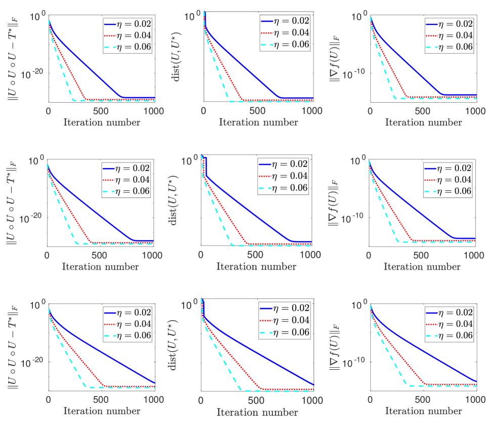
Figure 1: Linear convergence of gradient descent when applied to tensor factorization problem (6). Here, $r=n/2$ (top row), $r=n$ (middle row), and $r=3n/2$ (bottom row) with $n=64$. We initialize the starting point as $U^{\star}+\alpha D$ with $\alpha=0.07$ and set $D$ as a normalized Gaussian matrix with $\|D\|_{F}=1$. We record the three metrics $\|\nabla f(U)\|_{F}$ (left column), $\|U\circ U\circ U-T^{\star}\|_{F}$ (middle column), and ${\operatorname{dist}}(U,U^{\star})$ (right column) for total $10^{3}$ iterations with different stepsize $\eta$, which is consistent with the linear convergence analysis of gradient descent on general Burer-Monteiro tensor optimizations.

In the second experiment, with the same settings as above except varying $\alpha$, we record the success rate by running 100 trials for each fixed $(r,\alpha)$-pair and declare one successful instance if the final iterate $U$ satisfies ${\operatorname{dist}}(U,U^{\star})\leq 10^{-3}$. We repeat these experiments for different $\alpha\in\{0.5,1,2,4,8,16\}$. Table 1 shows that when $\alpha$ is small enough ($\alpha\leq 2$), the success rate is 100% for all the undercomplete ($r=n/2$), complete ($r=n$), and overcomplete ($r=3n/2$) cases; and when $\alpha$ is comparatively large ($\alpha\in[4,8]$), the success rate degrades dramatically when $r$ increases. Finally, when $\alpha$ is larger than certain threshold, the success rate is 0%. This in consistence with Corollaries 1 and 2.

Table 1: Success ratio with $\eta=0.02$ (top), $\eta=0.04$ (middle), and $\eta=0.06$ (bottom).

$\alpha$	0.5	1	2	4	8	16
$r=n/2$	100%	100%	100%	100%	100%	0%
$r=n$	100%	100%	100%	100%	100%	0%
$r=3n/2$	100%	100%	100%	100%	5%	0%

$\alpha$	0.5	1	2	4	8	16
$r=n/2$	100%	100%	100%	100%	100%	0%
$r=n$	100%	100%	100%	100%	0%	0%
$r=3n/2$	100%	100%	100%	100%	0%	0%

$\alpha$	0.5	1	2	4	8	16
$r=n/2$	100%	100%	100%	100%	38%	0%
$r=n$	100%	100%	100%	100%	0%	0%
$r=3n/2$	100%	100%	100%	83%	0%	0%

5 Conclusion

In this work, we investigated the local convergence of third-order tensor optimization with general convex and well-conditioned objective functions. Under certain incoherent conditions, we proved the local regularity condition for the nonconvex factored tensor optimization resulted from the Burer-Monteiro reparameterization. We highlighted that these assumptions are satisfied for randomly generated tensor factors. With this local regularity condition, we further provided a linear convergence analysis for the gradient descent algorithm started in a neighborhood of the true tensor factors. Complimentary to the local analysis, we also presented a complete characterization of the global optimization landscape of the best rank-one tensor approximation problem.

Appendix A Proof of Theorem 1

For convenience, we present all the necessary tensor/matrix notations in Table 2, where we assume $U=[{\boldsymbol{u}}_{1}~{}{\boldsymbol{u}}_{2}~{}\cdots~{}{\boldsymbol{u}}_{r}]\in\mathbb{R}^{n\times r}$, $V=[{\boldsymbol{v}}_{1}~{}{\boldsymbol{v}}_{2}~{}\cdots~{}{\boldsymbol{v}}_{r}]\in\mathbb{R}^{m\times r}$, and $W=[{\boldsymbol{w}}_{1}~{}{\boldsymbol{w}}_{2}~{}\cdots~{}{\boldsymbol{w}}_{r}]\in\mathbb{R}^{l\times r}$.

Table 2: Tensor/matrix notations

Symbols	Meaning	Explanation
$\otimes$	outer/tensor product	${\boldsymbol{u}}\otimes{\boldsymbol{v}}\otimes{\boldsymbol{w}}\doteq T\in\mathbb{R}^{n\times m\times l}$ with $T_{ijk}=u_{i}v_{j}w_{k}$.
$\circ$	group tensor product	$U\circ V=UV^{\top}$; $U\circ V\circ W\doteq\sum_{j=1}^{r}{\boldsymbol{u}}_{j}\otimes{\boldsymbol{v}}_{j}\otimes{\boldsymbol{w}}_{j}$ .
$\bigotimes$	Kronecker products	$U\bigotimes V\doteq\begin{bmatrix}u_{11}V&\cdots&u_{1r}V\\ \vdots&\ddots&\vdots\\ u_{n}V&\cdots&u_{nr}V\end{bmatrix}\in\mathbb{R}^{nm\times r^{2}}$.
$\circledast$	Khatri-Rao product	$U\circledast V\doteq\begin{bmatrix}{\boldsymbol{u}}_{1}\bigotimes{\boldsymbol{v}}_{1}&\cdots&{\boldsymbol{u}}_{m}\bigotimes{\boldsymbol{v}}_{m}\end{bmatrix}\in\mathbb{R}^{nm\times r}$ .
$\odot$	Hadamard product	$U\odot V\doteq M$ with $M_{ij}=u_{ij}v_{ij}$ when $m=n$.

To prove Theorem 1, we need the following key lemmas.

Lemma 2.

Denote $H\doteq U-U^{\star}P_{U}$ and assume $\|H\|_{F}\leq 0.07\frac{\underline{c}}{\omega^{3}}$. Under Assumptions 1-4, if $r=O(n^{1.25})$, we have the following bounds hold for sufficiently large $n$:

$$1.679\underline{c}^{4}\|H\|_{F}^{2}\leq\|T-T^{\star}\|_{F}^{2}\leq 10.336\omega^{4}\underline{c}^{4}\|H\|_{F}^{2}.$$

Lemma 3.

Suppose that a $(r,m,M)$-restricted strongly convex and smooth function $f:\mathbb{R}^{n\times n\times n}\rightarrow\mathbb{R}$ has a unique global minimizer at $T^{\star}$ of rank at most $r$. Then for any $\eta\leq\frac{1}{18\|[\nabla f(T)]_{(1)}\|\|U\|+9M\|U\|^{4}},$ we have

$$\langle\nabla f(U\circ U\circ U),U\circ U\circ U-T^{\star}\rangle\geq\frac{1}{2}\eta\|\nabla_{U}f(U\circ U\circ U)\|_{F}^{2}+\frac{m}{2}\|U\circ U\circ U-T^{\star}\|^{2}_{F}.$$

Lemma 4.

Suppose that a $(r,m,M)$-restricted strongly convex and smooth function $f:\mathbb{R}^{n\times n\times n}\rightarrow\mathbb{R}$ has a unique global minimizer at $T^{\star}$ of rank at most $r$. Then for any $T$ with ${\operatorname{rank}}(T)\leq r$, we have

$$\|\nabla f(T)\|_{F}=\|\nabla f(T)-\nabla f(T^{\star})\|_{F}\leq M\|T-T^{\star}\|_{F}.$$

Lemma 5.

For any two matrices $A=[{\boldsymbol{a}}_{1}~{}\cdots~{}{\boldsymbol{a}}_{r}]\in\mathbb{R}^{n\times r}$, $B=[{\boldsymbol{b}}_{1}~{}\cdots~{}{\boldsymbol{b}}_{r}]\in\mathbb{R}^{n\times r}$ and a tensor $C\in\mathbb{R}^{n\times n\times n}$, we have the following inequality holds

$$|\langle C,A\circ B\circ B\rangle|\leq\|C\|\cdot\max_{j\in[r]}\|{\boldsymbol{a}}_{j}\|_{2}\cdot\|B\|_{F}^{2}.$$

Proof of Theorem 1.

Observe that

$$\langle\nabla_{U}f,U-U^{\star}P_{U}\rangle= \langle 3[\nabla f]_{(1)}(T)U\circledast U,U-U^{\star}P_{U}\rangle$$

$$= 3\langle[\nabla f]_{(1)}(T),U(U\circledast U)^{T}-U^{\star}P_{U}(U\circledast U)^{T}\rangle$$

$$= 3\langle\nabla f(T),T-U^{\star}P_{U}\circ U\circ U\rangle\text{ (Denote new $U^{\star}=U^{\star}P_{U}.$)}$$

$$= \langle\nabla f(T),(T-T^{\star})+2(U-U^{\star})\circ(U-U^{\star})\circ(U-U^{\star})+3U^{\star}\circ(U-U^{\star})\circ(U-U^{\star})\rangle$$

$$= \langle\nabla f(T),(T-T^{\star})+2H\circ H\circ H+3U^{\star}\circ H\circ H\rangle$$

$$= \langle\nabla f(T),T-T^{\star}\rangle+\langle\nabla f(T),2H\circ H\circ H\rangle+\langle\nabla f(T),3U^{\star}\circ H\circ H\rangle.$$

Next, we bound the above three terms in sequence. Using Lemma 3, the first term can be bounded with

$$\langle\nabla f(T),T-T^{\star}\rangle\geq\frac{1}{2}\eta\|\nabla_{U}f\|_{F}^{2}+\frac{m}{2}\|T-T^{\star}\|^{2}_{F}.$$

Combining Lemmas 4 and 5, the absolute value of the last two terms can be bounded with

$$|\langle\nabla f(T),2H\circ H\circ H\rangle|\leq 2\|\nabla f(T)\|\|H\|_{F}^{3}$$

$$\leq 2M\|T-T^{\star}\|_{F}\|H\|_{F}^{3},$$

$$|\langle\nabla f(T),3U^{\star}\circ H\circ H\rangle|\leq 3\bar{c}\|\nabla f(T)\|\|H\|_{F}^{2}$$

$$\leq 3\bar{c}M\|T-T^{\star}\|_{F}\|H\|_{F}^{2}.$$

Then, we have

$$\langle\nabla_{U}f,U-U^{\star}P_{U}\rangle \geq\frac{1}{2}\eta\|\nabla_{U}f\|_{F}^{2}+\bigg{(}\frac{m}{2}\|T-T^{\star}\|_{F}^{2}-2M\|T-T^{\star}\|_{F}\|H\|_{F}^{3}-3M\bar{c}\|T-T^{\star}\|_{F}\|H\|_{F}^{2}\bigg{)}$$

$$\doteq\frac{1}{2}\eta\|\nabla_{U}f\|_{F}^{2}+\Pi.$$

Applying Lemma 2, we obtain

$$\Pi \geq\frac{1}{2}\bigg{(}1.679m\underline{c}^{2}-4\sqrt{10.336}M\omega^{2}\|H\|_{F}^{2}-6\sqrt{10.336}M\omega^{3}\underline{c}\|H\|_{F}\bigg{)}\underline{c}^{2}\|H\|_{F}^{2}$$

$$\geq\bigg{(}1.679-2\sqrt{10.336}\bigg{(}\frac{2(0.07)^{2}}{\omega^{4}}\cdot\frac{m}{M}+3(0.07)\bigg{)}\bigg{)}\frac{1}{2}m\underline{c}^{4}\|H\|_{F}^{2}$$

$$\geq\bigg{(}1.679-2\sqrt{10.336}(2(0.07)^{2}+3(0.07))\bigg{)}\frac{1}{2}m\underline{c}^{4}\|H\|_{F}^{2}$$

$$\geq 0.13m\underline{c}^{4}\|H\|_{F}^{2},$$

where the second inequality follows from $\|H\|_{F}\leq 0.07\frac{\underline{c}}{\omega^{3}}$. Finally, we can get the local regularity condition

$$\langle\nabla_{U}f,U-U^{\star}P_{U}\rangle\geq\frac{1}{2}\eta\|\nabla_{U}f\|_{F}^{2}+0.13m\underline{c}^{4}{\operatorname{dist}}(U,U^{\star})^{2}$$

and complete the proof of Theorem 1. ∎

Appendix B Proof of Corollaries 1 and 2

We first prove 1 by using the results stated in Theorem 1. In particular, we have

$${\operatorname{dist}}(U^{+},U^{\star})^{2}\leq \|U^{+}-U^{\star}P_{U}\|_{F}^{2}$$

$$= \|U^{+}-U+U-U^{\star}P_{U}\|_{F}^{2}$$

$$= \|U^{+}-U\|_{F}^{2}+\|U-U^{\star}P_{U}\|_{F}^{2}+2\langle U^{+}-U,U-U^{\star}P_{U}\rangle$$

$$= \eta^{2}\|\nabla_{U}f(U\circ U\circ U)\|_{F}^{2}+{\operatorname{dist}}(U,U^{\star})^{2}-2\eta\langle\nabla_{U}f(U\circ U\circ U),U-U^{\star}P_{U}\rangle$$

$$\leq \eta^{2}\|\nabla_{U}f(U\circ U\circ U)\|_{F}^{2}+{\operatorname{dist}}(U,U^{\star})^{2}-2\eta\bigg{(}\frac{1}{2}\eta\|\nabla_{U}f(U\circ U\circ U)\|_{F}^{2}+0.13m\underline{c}^{4}{\operatorname{dist}}(U,U^{\star})^{2}\bigg{)}$$

$$\leq (1-0.26\eta m\underline{c}^{4}){\operatorname{dist}}(U,U^{\star})^{2}.$$

Next, we continue to prove 2. With 1, it suffices to show that there is a stepsize $\eta_{0}$ such that

$$\eta_{0}\leq\min\left\{\frac{1}{18\|[\nabla f(U^{t}\circ U^{t}\circ U^{t})]_{(1)}\|\cdot\|U^{t}\|+9M\|U^{t}\|^{4}}\doteq s(U^{t}):~{}\forall t\geq 0\right\}.$$ (21)

For this purpose, we need to find an upper bound for $\|U^{t}\|$ and $\|[\nabla f(U^{t}\circ U^{t}\circ U^{t})]_{(1)}\|$.

We first bound $\|U^{t}\|$. Note that $U^{0}$ lies in the local region if $\eta$ is small enough. Then, for any current variable $U^{t}$, we have

$$\max\{\|U^{0}-U^{\star}\|_{F},\|U^{t}-U^{\star}\|_{F}\}\leq 0.07\frac{m}{M}\frac{\underline{c}}{\omega^{3}}\leq 0.07\underline{c}\leq 0.07\|U^{\star}\|,$$ (22)

which implies that

$$\max\{\|U^{0}-U^{\star}\|,\|U^{t}-U^{\star}\|\}\leq 0.07\|U^{\star}\|,$$

and

$$0.93\|U^{\star}\|\leq\max\{\|U^{t}\|,\|U^{0}\|\}\leq 1.07\|U^{\star}\|.$$

Thus, we can get

$$\|U^{t}\|\leq\frac{1.07}{0.93}\|U^{0}\|\text{ and }\bar{c}\leq\|U^{\star}\|\leq\frac{1}{0.93}\|U^{0}\|,$$ (23)

where the first part follows from $\|U\|\leq 1.07\|U^{\star}\|$ and $\|U^{\star}\|\leq\frac{1}{0.93}\|U^{0}\|$, and the second line follows from $\|U^{\star}\|\leq\frac{1}{0.93}\|U^{0}\|$, $\|U^{\star}\|\geq\max_{i}\|{\boldsymbol{u}}_{i}^{\star}\|_{2}$, and $\bar{c}\doteq\max_{i}\|{\boldsymbol{u}}_{i}^{\star}\|_{2}$.

Next, we bound $\|[\nabla f(U^{t}\circ U^{t}\circ U^{t})]_{(1)}\|$, or equivalently $\|[\nabla f(T)]_{(1)}\|$ with $T=U^{t}\circ U^{t}\circ U^{t}$. Observe that

$$\|[\nabla f(T)]_{(1)}\| \leq\|\nabla f(T)\|_{F}$$ (24)

$$\leq M\|T-T^{\star}\|$$

$$\leq(10.336)^{1/2}M\bar{c}^{2}\|U^{t}-U^{\star}\|_{F}$$

$$\leq(10.336)^{1/2}M\bar{c}^{2}\bigg{(}\frac{0.07}{0.93}\|U^{0}\|\bigg{)}$$

$$\leq 0.242M\bar{c}^{2}\|U^{0}\|,$$ (25)

where the second inequality follows from Lemma 4, the third inequality follows from Lemma 2, and the fourth inequality follows from (22) and (23).

Finally, plugging the upper bound of $\|U^{t}\|$ in (23) and the upper bound of $\|[\nabla f(T)]_{(1)}\|$ in (25) to the definition of $s(U^{t})$, i.e.,

$$s(U^{t})\doteq\frac{1}{18\|[\nabla f(U^{t}\circ U^{t}\circ U^{t})]_{(1)}\|\cdot\|U^{t}\|+9M\|U^{t}\|^{4}},$$

we can bound $s(U^{t})$ as

$$s(U^{t}) \geq\frac{1}{18(0.242M(\frac{1}{0.93}\|U^{0}\|)^{2}\|U^{0}\|)(\frac{1.07}{0.93}\|U^{0}\|)+9M(\frac{1.07}{0.93}\|U^{0}\|)^{4}}\geq\frac{1}{21.6M\|U^{0}\|^{4}}.$$

Therefore, we complete the proof of 2.

Appendix C Proof of Lemmas 2 and 3

To prove Lemmas 2 and 3, we require some additional auxiliary lemmas.

C.1 Auxiliary lemmas

We first introduce the auxiliary lemmas used for proving 2, which are mainly related with Assumptions 1-3. Since Assumptions 1-3 are concerned with the normalized factors $\widehat{U}$, we need transform these assumptions to apply to $U^{\star}$ by using that the dynamic range of the coefficients $\{c_{j}^{\star 1/3}\}$ is small.

Lemma 6.

Under 1 on $\widehat{U}$, the mutual incoherence coefficient of $U^{\star}$ is upper bounded by

$$\mu^{\star}=\max_{i\neq j}|\langle{{\boldsymbol{u}}}_{i}^{\star},{{\boldsymbol{u}}}_{j}^{\star}\rangle|\leq\frac{\bar{c}^{2}\gamma}{\sqrt{n}}.$$ (26)

Proof of 6.

By 1, we have

$$\max_{i\neq j}|\langle\widehat{{\boldsymbol{u}}}_{i},\widehat{{\boldsymbol{u}}}_{j}\rangle|\leq\frac{\gamma}{\sqrt{n}}.$$

Since ${\boldsymbol{u}}^{\star}_{i}={c_{i}^{\star}}^{1/3}\widehat{{\boldsymbol{u}}}_{i}$ for any $i\neq j$, we have

$$|\langle{\boldsymbol{u}}^{\star}_{i},{\boldsymbol{u}}^{\star}_{j}\rangle|= {c_{i}^{\star}}^{1/3}{c_{j}^{\star}}^{1/3}|\langle\widehat{{\boldsymbol{u}}}_{i},\widehat{{\boldsymbol{u}}}_{j}\rangle|$$

$$\leq \big{(}\max_{k\in[r]}{c_{k}^{\star}}^{1/3}\big{)}^{2}\cdot\max_{i\neq j}|\langle\widehat{{\boldsymbol{u}}}_{i},\widehat{{\boldsymbol{u}}}_{j}\rangle|$$

$$= \bar{c}^{2}\cdot\frac{\gamma}{\sqrt{n}}$$

∎

Lemma 7.

Under 2 on $\widehat{U}$, the operator norm of $U^{\star}$ is bounded by

$$\|U^{\star}\|\leq\bar{c}\bigg{(}1+c_{1}\sqrt{\frac{r}{n}}\bigg{)}.$$ (27)

Proof of 7.

By 2 on $\widehat{U}$, we have

$$\|\widehat{U}\|\leq 1+c_{1}\sqrt{\frac{r}{n}}.$$

This along with ${\boldsymbol{u}}^{\star}_{i}=c_{i}^{1/3}\widehat{{\boldsymbol{u}}}_{i}$ implies that

$$U^{\star}=\widehat{U}\underbrace{\begin{bmatrix}{c_{1}^{\star}}^{1/3}&0&\cdots&0\\ 0&{c_{2}^{\star}}^{1/3}&\cdots&0\\ \vdots&\vdots&\vdots&\vdots\\ 0&\cdots&0&{c_{r}^{\star}}^{1/3}\end{bmatrix}}_{C}.$$

Therefore,

$$\|U^{\star}\| \leq\|\widehat{U}\|\cdot\|C\|$$

$$\leq(1+c_{1}\sqrt{\frac{r}{n}})\cdot\max_{k\in[r]}{c_{k}^{\star}}^{1/3}$$

$$=(1+c_{1}\sqrt{\frac{r}{n}})\cdot\bar{c}.$$

The second inequality follows from 2 on $\widehat{U}$, and the fact that the operator norm of a diagonal matrix is the largest absolute value of its diagonal entries. ∎

Further, we claim that the $2\rightarrow 3$ norm and $2\rightarrow 4$ norm of $U^{\star}$ are also upper bounded under 1, where the general $p\to q$ norm is denoted and defined by $\|A\|_{p\to q}\doteq\max_{{\boldsymbol{x}}\neq\mathbf{0}}\frac{\|A{\boldsymbol{x}}\|_{q}}{\|{\boldsymbol{x}}\|_{p}}.$

In particular, we have the following lemma.

Lemma 8.

Under 1 on $\widehat{U}$, the $2\rightarrow 3$ norm and $2\rightarrow 4$ norm of $U^{\star}$ are bounded with

$$\|{U^{\star}}^{\top}\|^{k}_{2\rightarrow 3}\leq\bar{c}^{k}\big{(}1+O(\gamma n^{-\epsilon})\big{)},\quad{\operatorname{if}}~{}r=O(n^{1.25-1.5\epsilon}),$$

$$\|{U^{\star}}^{\top}\|^{k}_{2\rightarrow 4}\leq\bar{c}^{k}\big{(}1+O(\gamma n^{-\epsilon})\big{)},\quad{\operatorname{if}}~{}r=O(n^{1.5-2\epsilon}).$$

Proof of 8.

It suffices to show

$$\|{\widehat{U}}^{\top}\|_{2\rightarrow 3} \leq 1+O(\gamma n^{-\epsilon}),\quad{\operatorname{if}}~{}r=O(n^{1.25-1.5\epsilon}),$$

$$\|{\widehat{U}}^{\top}\|_{2\rightarrow 4} \leq 1+O(\gamma n^{-\epsilon}),\quad{\operatorname{if}}~{}r=O(n^{1.5-2\epsilon}).$$

First of all, identify that

$$\|{U^{\star}}^{\top}\|_{2\rightarrow 3} =\|\widehat{U}C\|_{2\rightarrow 3}$$

$$\leq\|\widehat{U}\|_{2\rightarrow 3}\cdot\|C\|$$

$$\leq\big{(}1+O(\gamma n^{-\epsilon})\big{)}\cdot\bar{c},$$

where the second inequality is because

$$\|AB\|_{2\rightarrow 3} =\max_{\|{\boldsymbol{x}}\|_{2}=1}\|AB{\boldsymbol{x}}\|_{3}$$

$$\leq\|A\|_{2\rightarrow 3}\cdot\max_{\|{\boldsymbol{x}}\|_{2}=1}\|Bx\|_{2}$$

$$=\|A\|_{2\rightarrow 3}\cdot\|B\|.$$

Since

$$\big{(}1+O(\gamma n^{-\epsilon})\big{)}^{k}=1+O(\gamma n^{-\epsilon}),$$

we have

$$\|{U^{\star}}^{\top}\|^{k}_{2\rightarrow 3}\leq\bar{c}^{k}\big{(}1+O(\gamma n^{-\epsilon})\big{)}.$$

A similar argument applies to $\|{U^{\star}}^{\top}\|^{k}_{2\rightarrow 4}\leq\bar{c}^{k}\big{(}1+O(\gamma n^{-\epsilon})\big{)}$.

Therefore, to complete this proof, it suffices to show

$$\|{\widehat{U}}^{\top}\|_{2\rightarrow 3} \leq 1+O(\gamma n^{-\epsilon}),\quad{\operatorname{if}}~{}r=O(n^{1.25-1.5\epsilon}),$$

$$\|{\widehat{U}}^{\top}\|_{2\rightarrow 4} \leq 1+O(\gamma n^{-\epsilon}),\quad{\operatorname{if}}~{}r=O(n^{1.5-2\epsilon}),$$

which are clearly true when $\|{\widehat{U}}^{\top}\|_{2\rightarrow p}\leq 1$ with $p=3,4$.

We continue to consider the case when $\|{\widehat{U}}^{\top}\|_{2\rightarrow p}>1$ with $p=3,4$. Note that

$$\|{\widehat{U}}^{\top}\|_{2\rightarrow p}\leq \|{\widehat{U}}^{\top}\|_{2\rightarrow p}^{p}=\sup_{\|{\boldsymbol{x}}\|_{2}=1}\|{\widehat{U}}^{\top}{\boldsymbol{x}}\|^{p}_{p}.$$

Take arbitrary ${\boldsymbol{x}}\in\mathbb{S}^{n-1}$, the unit sphere in $\mathbb{R}^{n}$. Denoting $S$ as the indices of the largest $L$ entries in ${\widehat{U}}^{\top}{\boldsymbol{x}}$, we have

$$\|{\widehat{U}}^{\top}{\boldsymbol{x}}\|_{p}^{p}=\|{\widehat{U}}_{S}^{\top}{\boldsymbol{x}}\|_{p}^{p}+\|{\widehat{U}}_{S^{c}}^{\top}{\boldsymbol{x}}\|_{p}^{p}.$$

Next, we bound the above two terms sequentially.

• For the first term, we have

  $$\|{\widehat{U}}_{S}^{\top}{\boldsymbol{x}}\|_{p}^{p} \leq\|{\widehat{U}}_{S}^{\top}{\boldsymbol{x}}\|_{2}^{2}$$

  $$\leq\|{\widehat{U}}_{S}\|^{2}\cdot\|{\boldsymbol{x}}\|_{2}^{2}$$

  $$=\|{\widehat{U}}_{S}{\widehat{U}}_{S}^{\top}\|\leq 1+\sum_{i\neq j}|\langle\widehat{{\boldsymbol{u}}}_{i},\widehat{{\boldsymbol{u}}}_{j}\rangle|$$

  $$\leq 1+O\left(\frac{L\gamma}{\sqrt{n}}\right),$$

  where the first inequality holds since $({\widehat{U}}_{S}^{\top}{\boldsymbol{x}})_{i}\leq 1$, the fourth inequality follows from the Disk Theorem for symmetric matrix, and the fifth inequality follows from 1.

• For the second term, note that

  $$\min_{i\in S}|\widehat{{\boldsymbol{u}}}_{i}^{\top}{\boldsymbol{x}}|^{2} \leq\frac{1}{L}\|{\widehat{U}}_{S}{\widehat{U}}^{\top}_{S}\|\|{\boldsymbol{x}}\|^{2}$$

  $$\leq\frac{1}{L}\bigg{(}1+O\left(L\frac{\gamma}{\sqrt{n}}\right)\bigg{)}$$

  $$=O\left(\frac{1}{L}\right),$$

  where we assume

  $$\frac{\gamma}{\sqrt{n}}=o\left(\frac{1}{L}\right)\text{ or }L=o\left(\frac{\sqrt{n}}{\gamma}\right).$$

  Choosing a support $S$ such that $\max_{i\in S^{c}}|\widehat{{\boldsymbol{u}}}_{i}^{\top}{\boldsymbol{x}}|^{2}\leq O(\frac{1}{L}).$ Then, we have

  $$\|{\widehat{U}}_{S^{c}}^{\top}{\boldsymbol{x}}\|_{p}^{p} =\sum_{i\notin S}|\widehat{{\boldsymbol{u}}}_{i}^{\top}{\boldsymbol{x}}|^{p}$$

  $$\leq\big{(}\max_{i\notin S}|\widehat{{\boldsymbol{u}}}_{i}^{\top}{\boldsymbol{x}}|^{p-2}\big{)}\sum_{i\notin S}|\widehat{{\boldsymbol{u}}}_{i}^{\top}{\boldsymbol{x}}|^{2}$$

  $$\leq O(L^{1-0.5p})\|{\widehat{U}}_{S^{c}}^{\top}{\boldsymbol{x}}\|_{2}^{2}$$

  $$\leq O(L^{1-0.5p}rn^{-1}),$$

  where the third inequality holds since $\max_{i\in S^{c}}|\widehat{{\boldsymbol{u}}}_{i}^{\top}{\boldsymbol{x}}|^{2}\leq O(\frac{1}{L})$, and the last inequality follows from

  $$\|{\widehat{U}}_{S^{c}}^{\top}{\boldsymbol{x}}\|_{2}^{2}\leq\|U\|^{2}\leq(1+c\sqrt{\frac{r}{n}})^{2}=O(\frac{r}{n}),$$

  which is a consequence of 2. Therefore, when $p=3$, we get

  $$\|{\widehat{U}}_{S^{c}}^{\top}{\boldsymbol{x}}\|_{3}^{3}\leq O(L^{-0.5}rn^{-1}).$$

Combining these two terms, we have

$$\|{\widehat{U}}^{\top}{\boldsymbol{x}}\|_{3}^{3}\leq 1+O(L{\gamma}/{\sqrt{n}})+O(L^{-0.5}rn^{-1}),$$

which can be further optimized by carefully choosing $L$ and $r$.

In particular, let us consider the following optimization:

$$\min_{r\gg n,L}\max~{}\big{\{}O(L{\gamma}/{\sqrt{n}}),O(L^{-0.5}rn^{-1})\big{\}}.$$

Choosing $L=O({n^{0.5-r_{c}}}/\gamma),$ and $r=O(n^{1+\beta})$, we get

$$\big{\{}O(L\gamma/{\sqrt{n}}),O(L^{-0.5}rn^{-1})\big{\}} =\big{\{}O(n^{-r_{c}}),O(\gamma^{0.5}n^{-1.25+0.5r_{c}}r)\big{\}}$$

$$=\big{\{}O(n^{-r_{c}}),O(\gamma^{0.5}n^{-0.25+0.5r_{c}+\beta})\big{\}}$$

$$=\big{\{}O(n^{-r_{c}}),O(n^{-r_{c}}{\operatorname{polylog}}(n)^{0.5})\big{\}},$$

where the last equality follows by setting $-r_{c}=-0.25+0.5r_{c}+\beta\text{ or }\beta=0.25-1.5r_{c}$. It follows that

$$\|{\widehat{U}}^{\top}{\boldsymbol{x}}\|_{3}^{3}\leq 1+O(\gamma n^{-r_{c}}),$$

when $r=O(n^{1.25-1.5r_{c}})$. Since the above inequality holds for any ${\boldsymbol{x}}\in\mathbb{S}^{n-1}$, we have

$$\max_{{\boldsymbol{x}}\in\mathbb{S}^{n-1}}\|{\widehat{U}}^{\top}{\boldsymbol{x}}\|_{3}^{3} \leq 1+O(\operatorname*{\gamma}n^{-r_{c}})$$

when provided with $r=O(n^{1.25-1.5r_{c}})$. Then, we obtain

$$\|{\widehat{U}}^{\top}\|_{2\rightarrow 3}^{3}\leq 1+O(\operatorname*{\gamma}n^{-r_{c}}),$$

which further implies that

$$\|{\widehat{U}}^{\top}\|_{2\rightarrow 3}\leq 1+O(\operatorname*{\gamma}n^{-r_{c}}),$$

when provided with $r=O(n^{1.25-1.5r_{c}})$.

With a similar argument, we can also show that

$$\|{\widehat{U}}^{\top}\|_{2\rightarrow 4}\leq 1+O({\operatorname{polylog}}(n)n^{-r_{c}})$$

when provided with $r=O(n^{1.5-2r_{c}})$. ∎

Lemma 9.

Under 3 on $\widehat{U}$, we have

$$\lambda_{\min}(({{U^{\star}}^{\top}}{U^{\star}})\odot({{U^{\star}}^{\top}}{U^{\star}})) \geq\underline{c}^{4}(1-\frac{\gamma\sqrt{r}}{n}),$$

$$\lambda_{\max}(({{U^{\star}}^{\top}}{U^{\star}})\odot({{U^{\star}}^{\top}}{U^{\star}})) \leq\bar{c}^{4}(1+\frac{\gamma\sqrt{r}}{n}).$$ (28)

Proof.

From 3, we have

$$\|(\widehat{U}^{\top}\widehat{U})\odot({\widehat{U}}^{\top}\widehat{U})-I_{r}\|\leq\frac{\gamma\sqrt{r}}{n}.$$

Since the operator norm of a symmetric matrix equals the largest absolute eigenvalues and

$$\max_{i\in[r]}|\lambda_{i}((\widehat{U}^{\top}\widehat{U})\odot({\widehat{U}}^{\top}\widehat{U})-I)|=\max_{i\in[r]}|\lambda_{i}((\widehat{U}^{\top}\widehat{U})\odot({\widehat{U}}^{\top}\widehat{U}))-1|,$$

we have

$$\max_{i\in[r]}|\lambda_{i}((\widehat{U}^{\top}\widehat{U})\odot({\widehat{U}}^{\top}\widehat{U}))-1|\leq\frac{\gamma\sqrt{r}}{n},$$

implying

$$|\lambda_{i}((\widehat{U}^{\top}\widehat{U})\odot({\widehat{U}}^{\top}\widehat{U}))-1|\leq\frac{\gamma\sqrt{r}}{n},i\in[r].$$

Hence, we get

$$1-\frac{\gamma\sqrt{r}}{n}\leq\lambda_{i}((\widehat{U}^{\top}\widehat{U})\odot({\widehat{U}}^{\top}\widehat{U}))\leq 1+\frac{\gamma\sqrt{r}}{n}.$$

Next, we derive the lower bound and upper bound for $\lambda_{i}({{U^{\star}}^{\top}}U^{\star}\odot{{U^{\star}}^{\top}}U^{\star})$. Observe that

$$\bigg{[}(\widehat{U}^{\top}\widehat{U})\odot({\widehat{U}}^{\top}\widehat{U})\bigg{]}_{i,j} =(\widehat{{\boldsymbol{u}}}_{i}^{\top}\widehat{{\boldsymbol{u}}}_{j})^{2},$$

$$\bigg{[}({{U^{\star}}^{\top}}{U^{\star}})\odot({{U^{\star}}^{\top}}{U^{\star}})\bigg{]}_{i,j} ={c_{i}^{\star}}^{2/3}{c_{j}^{\star}}^{2/3}(\widehat{{\boldsymbol{u}}}_{i}^{\top}\widehat{{\boldsymbol{u}}}_{j})^{2}.$$

Then, we have

$$\lambda_{\min}(({{U^{\star}}^{\top}}{U^{\star}})\odot({{U^{\star}}^{\top}}{U^{\star}}))= \min_{\|{\boldsymbol{x}}\|_{2}=1}{\boldsymbol{x}}^{\top}(({{U^{\star}}^{\top}}{U^{\star}})\odot({{U^{\star}}^{\top}}{U^{\star}})){\boldsymbol{x}}$$

$$= \min_{\|{\boldsymbol{x}}\|_{2}=1}\sum_{i,j\in[r]}{c_{i}^{\star}}^{2/3}{c_{j}^{\star}}^{2/3}x_{i}x_{j}(\widehat{{\boldsymbol{u}}}_{i}^{\top}\widehat{{\boldsymbol{u}}}_{j})^{2}$$

$$\geq \min_{i\in[r]}{c_{i}^{\star}}^{4/3}\cdot\min_{\|{\boldsymbol{x}}\|_{2}=1}\sum_{i,j\in[r]}x_{i}x_{j}(\widehat{{\boldsymbol{u}}}_{i}^{\top}\widehat{{\boldsymbol{u}}}_{j})^{2}$$

$$= \underline{c}^{4}\cdot\lambda_{\min}((\widehat{U}^{\top}\widehat{U})\odot({\widehat{U}}^{\top}\widehat{U})).$$

Similarly, we can obtain

$$\lambda_{\max}(({{U^{\star}}^{\top}}{U^{\star}})\odot({{U^{\star}}^{\top}}{U^{\star}})) \leq\bar{c}^{4}\cdot\lambda_{\max}((\widehat{U}^{\top}\widehat{U})\odot({\widehat{U}}^{\top}\widehat{U})).$$

This completes the proof of Lemma 9. ∎

Lemma 10.

For any $n\times n$ symmetric semi-definite matrices $A$, $B$, we have

$$\langle A,B\rangle\leq\min\{\|B\|{\operatorname{trace}}(A),\|A\|{\operatorname{trace}}(B)\}.$$ (29)

Proof.

Due to symmetry, we only prove $\langle A,B\rangle\leq\|B\|{\operatorname{trace}}(A)$. Denote the eigenvalues of $A$ as $\lambda_{i}(A),i\in[n]$ and the eigenvalues of $B$ as $\lambda_{i}(B),i\in[n]$. Note that for a symmetric semidefinite matrix, the eigenvalues and the singular values are the same. Then, by Von Neumann’s trace inequality, we obtain

$$\langle A,B\rangle \leq\sum_{i\in[n]}\lambda_{i}(A)\lambda_{i}(B)$$

$$\leq\lambda_{\max}(B)\sum_{i\in[n]}\lambda_{i}(A)$$

$$=\|B\|{\operatorname{trace}}(A).$$

∎

Lemma 11.

For any $k\geq 2$, we have $\|AX\|_{k}\leq\|A\|_{2\rightarrow k}\|X\|_{F}$.

Proof.

Observe that

$$\|AX\|_{k}^{k} \leq\sum_{i}(\|A\|_{2\rightarrow k}\|{\boldsymbol{x}}_{i}\|_{2}^{k})$$

$$=\|A\|_{2\rightarrow k}^{k}\sum_{i}\|{\boldsymbol{x}}_{i}\|_{2}^{k}$$

$$\leq\|A\|^{k}_{2\rightarrow k}\|X\|_{F}^{k},$$

where the first inequality follows from the definition of $2\rightarrow k$ norm, and the last inequality holds since

$$\sum_{i}\|{\boldsymbol{x}}_{i}\|_{2}^{k} =\big{\|}[\|{\boldsymbol{x}}_{1}\|_{2}~{}\cdots~{}\|{\boldsymbol{x}}_{r}\|_{2}]\big{\|}_{k}^{k}$$

$$\leq\big{\|}[\|{\boldsymbol{x}}_{1}\|_{2}~{}\cdots~{}\|{\boldsymbol{x}}_{r}\|_{2}]\big{\|}_{2}^{k}$$

$$=\|X\|_{F}^{k}.$$

Here, the second inequality follows from the Hardy’s inequality that $\|{\boldsymbol{x}}\|_{k}\leq\|{\boldsymbol{x}}\|_{2}$ when $k\geq 2$. Therefore, we have $\|AX\|_{k}^{k}\leq\|A\|^{k}_{2\rightarrow k}\|X\|_{F}^{k}$ or $\|AX\|_{k}\leq\|A\|_{2\rightarrow k}\|X\|_{F}$. ∎

Lemma 12.

For any vectors $\mathbf{f},\mathbf{g},\mathbf{h}$ of the same size, we have

$$\sum_{i}|\mathbf{f}(i)\mathbf{g}(i)\mathbf{h}(i)|\leq\|\mathbf{f}\|_{3}\|\mathbf{g}\|_{3}\|\mathbf{h}\|_{3}.$$

Proof.

Denote ${\boldsymbol{x}}\doteq{\boldsymbol{g}}\odot{\boldsymbol{h}}$. We have

$$\sum_{i}|\mathbf{f}(i)\mathbf{g}(i)\mathbf{h}(i)|= |\langle{\boldsymbol{f}},{\boldsymbol{x}}\rangle|$$

$$\leq \|{\boldsymbol{f}}\|_{3}\|{\boldsymbol{x}}\|_{3/2}$$

$$= \|{\boldsymbol{f}}\|_{3}\left(\sum_{i}|{\boldsymbol{g}}(i)|^{3/2}|{\boldsymbol{h}}(i)|^{3/2}\right)^{2/3}$$

$$\leq \|{\boldsymbol{f}}\|_{3}\left(\sqrt{\sum_{i}|{\boldsymbol{g}}(i)|^{3}}\sqrt{\sum_{i}|{\boldsymbol{h}}(i)|^{3}}\right)^{2/3}$$

$$= \|{\boldsymbol{f}}\|_{3}\left(\sqrt{\|{\boldsymbol{g}}\|_{3}^{3}}\sqrt{\|{\boldsymbol{h}}\|_{3}^{3}}\right)^{2/3}$$

$$= \|{\boldsymbol{f}}\|_{3}\|{\boldsymbol{g}}\|_{3}\|{\boldsymbol{h}}\|_{3},$$

where the both inequalities follow from the Hölder’s inequality that $|\langle{\boldsymbol{a}},{\boldsymbol{b}}\rangle|\leq\|{\boldsymbol{a}}\|_{p}\|{\boldsymbol{b}}\|_{q}$ with $(p,q)=(3,3/2)$ and $(p,q)=(2,2)$, respectively. ∎

Now, we are ready to prove Lemmas 2 and 3.

C.2 Proof of Lemma 2

Upper bound for $\|T-T^{\star}\|_{F}^{2}$

First of all, we expand

$$T=U\circ U\circ U=(U^{\star}+H)\circ(U^{\star}+H)\circ(U^{\star}+H)$$

into 8 terms as

$$T-T^{\star} =(U^{\star}+H)\circ(U^{\star}+H)\circ(U^{\star}+H)-U^{\star}\circ U^{\star}\circ U^{\star}$$

$$=H\circ U^{\star}\circ U^{\star}+U^{\star}\circ H\circ U^{\star}+U^{\star}\circ U^{\star}\circ H+H\circ H\circ U^{\star}+H\circ U^{\star}\circ H+U^{\star}\circ H\circ H+H\circ H\circ H.$$

We then plug it into $\|T-T^{\star}\|_{F}^{2}$ and continue to expand it. With some simplification, we have

$$\|T-T^{\star}\|^{2}_{F}= \|\underbrace{\big{(}H\circ U^{\star}\circ U^{\star}+\cdots\big{)}}_{\#3}+\underbrace{\big{(}H\circ H\circ U^{\star}+\cdots\big{)}}_{\#3}+H\circ H\circ H\|_{F}^{2}$$

$$= 3\langle H^{\top}H,{U^{\star}}^{\top}U^{\star}\odot{U^{\star}}^{\top}U^{\star}\rangle$$ (Term-(1))

$$+6\langle{U^{\star}}^{\top}U^{\star},(H^{\top}U^{\star})\odot({U^{\star}}^{\top}H)$$ (Term-(2))

$$+6\langle H^{\top}{U^{\star}},({U^{\star}}^{\top}H)^{\odot 2}\rangle$$ (Term-(3))

$$+12\langle{U^{\star}}^{\top}H,H^{\top}H\odot{U^{\star}}^{\top}U^{\star}\rangle$$ (Term-(4))

$$+6\langle H^{\top}H,({U^{\star}}^{\top}H)^{\odot 2}\rangle$$ (Term-(5))

$$+3\langle{U^{\star}}^{\top}U^{\star},(H^{\top}H)\odot(H^{\top}H)\rangle$$ (Term-(6))

$$+6\langle H^{\top}H,(H^{\top}U^{\star})\odot({U^{\star}}^{\top}H)\rangle$$ (Term-(7))

$$+6\langle{U^{\star}}^{\top}H,(H^{\top}H)\odot(H^{\top}H)\rangle$$ (Term-(8))

$$+\langle H^{\top}H,(H^{\top}H)\odot(H^{\top}H)\rangle,$$ (Term-(9))

where we use $U^{\odot 2}$ to denote $U\odot U$. Next, we bound the above nine terms sequentially.

• Term-(1): With Lemmas 9 and 10, the first term can be bounded with

  $$\langle H^{\top}H,{U^{\star}}^{\top}U^{\star}\odot{U^{\star}}^{\top}U^{\star}\rangle \leq\lambda_{\max}({U^{\star}}^{\top}U^{\star}\odot{U^{\star}}^{\top}U^{\star})\|H\|_{F}^{2}$$

  $$\leq\bar{c}^{4}\bigg{(}1+\frac{\gamma\sqrt{r}}{n}\bigg{)}\|H\|_{F}^{2}.$$

• Term-(2): Note that

  $$\langle{U^{\star}}^{\top}U^{\star},(H^{\top}U^{\star})\odot({U^{\star}}^{\top}H)= \sum_{i,j\in[r]}\langle{\boldsymbol{u}}^{\star}_{i},{\boldsymbol{u}}^{\star}_{j}\rangle\langle{\boldsymbol{h}}_{i},{\boldsymbol{u}}^{\star}_{j}\rangle\langle{\boldsymbol{u}}^{\star}_{i},{\boldsymbol{h}}_{j}\rangle$$

  $$= \underbrace{\sum_{i\neq j}\langle{\boldsymbol{u}}^{\star}_{i},{\boldsymbol{u}}^{\star}_{j}\rangle\langle{\boldsymbol{h}}_{i},{\boldsymbol{u}}^{\star}_{j}\rangle\langle{\boldsymbol{u}}^{\star}_{i},{\boldsymbol{h}}_{j}\rangle}_{\Pi_{1}}+\underbrace{\sum_{i\in[r]}\langle{\boldsymbol{u}}^{\star}_{i},{\boldsymbol{u}}^{\star}_{i}\rangle\langle{\boldsymbol{h}}_{i},{\boldsymbol{u}}^{\star}_{i}\rangle\langle{\boldsymbol{h}}_{i},{\boldsymbol{u}}^{\star}_{i}\rangle}_{\Pi_{2}}.$$

  We first bound $\Pi_{1}$ with

  $$\Pi_{1} \leq\sum_{i\neq j}\big{|}\langle{\boldsymbol{u}}^{\star}_{i},{\boldsymbol{u}}^{\star}_{j}\rangle\langle{\boldsymbol{h}}_{i},{\boldsymbol{u}}^{\star}_{j}\rangle\langle{\boldsymbol{u}}^{\star}_{i},{\boldsymbol{h}}_{j}\rangle\big{|}$$

  $$\leq\max_{i\neq j}\big{|}\langle{\boldsymbol{u}}^{\star}_{i},{\boldsymbol{u}}^{\star}_{j}\rangle\big{|}\cdot\sum_{i\neq j}\big{|}\langle{\boldsymbol{h}}_{i},{\boldsymbol{u}}^{\star}_{j}\rangle\langle{\boldsymbol{u}}^{\star}_{i},{\boldsymbol{h}}_{j}\rangle\big{|}$$

  $$\leq\mu^{\star}\cdot\langle\big{|}H^{\top}U^{\star}\big{|},\big{|}{U^{\star}}^{\top}H\big{|}\rangle$$

  $$\leq\mu^{\star}\cdot\|H^{\top}U^{\star}\|_{F}\|{U^{\star}}^{\top}H\|_{F}$$

  $$\leq\mu^{\star}\cdot\|U^{\star}\|^{2}\cdot\|H\|_{F}^{2},$$

  where the operation $|\cdot|$ on a matrix means taking the absolute value of all its entries. The last second inequality follows from the Cauchy-Schwarz’s inequality. The last inequality holds due to Lemma 11. We then bound $\Pi_{2}$ with

  $$\Pi_{2} \leq\max_{i\in[r]}\langle{\boldsymbol{u}}^{\star}_{i},{\boldsymbol{u}}^{\star}_{i}\rangle\cdot\sum_{i\in[r]}\langle{\boldsymbol{h}}_{i},{\boldsymbol{u}}^{\star}_{i}\rangle^{2}$$

  $$\leq\max_{i\in[r]}\|{\boldsymbol{u}}^{\star}_{i}\|_{2}^{2}\cdot\sum_{i\in[r]}\|{\boldsymbol{h}}_{i}\|_{2}^{2}\|{\boldsymbol{u}}^{\star}_{i}\|_{2}^{2}$$

  $$\leq\max_{i\in[r]}\|{\boldsymbol{u}}^{\star}_{i}\|_{2}^{4}\cdot\sum_{i\in[r]}\|{\boldsymbol{h}}_{i}\|_{2}^{2}$$

  $$=\bar{c}^{4}\cdot\|H\|_{F}^{2}.$$

  Combining the upper bound for $\Pi_{1}$ and $\Pi_{2}$, we obtain

  $$\langle{U^{\star}}^{\top}U^{\star},(H^{\top}U^{\star})\odot({U^{\star}}^{\top}H)\leq(\mu^{\star}\|U^{\star}\|^{2}+\bar{c}^{4})\cdot\|H\|_{F}^{2}.$$

• Term-(3): With Lemmas 11 and 12, we can bound the third term with

  $$\langle H^{\top}{U^{\star}},({U^{\star}}^{\top}H)\odot({U^{\star}}^{\top}H)\rangle \leq\|{U^{\star}}^{\top}H\|_{3}^{3}$$

  $$\leq\|{U^{\star}}^{\top}\|_{2\rightarrow 3}^{3}\|H\|_{F}^{3}.$$

• Term-(4): Note that

  $$\langle{U^{\star}}^{\top}H,H^{\top}H\odot{U^{\star}}^{\top}U^{\star}\rangle =\sum_{i\neq j}\langle{\boldsymbol{u}}^{\star}_{i},{\boldsymbol{h}}_{j}\rangle\langle{\boldsymbol{h}}_{i},{\boldsymbol{h}}_{j}\rangle\langle{\boldsymbol{u}}^{\star}_{i},{\boldsymbol{u}}^{\star}_{j}\rangle+\sum_{i}\langle{\boldsymbol{u}}^{\star}_{i},{\boldsymbol{h}}_{i}\rangle\langle{\boldsymbol{h}}_{i},{\boldsymbol{h}}_{i}\rangle\langle{\boldsymbol{u}}^{\star}_{i},{\boldsymbol{u}}^{\star}_{i}\rangle$$

  $$\doteq\Pi_{1}+\Pi_{2}.$$

  With a similar technique used in Term-(2), we can bound $\Pi_{1}$ and $\Pi_{2}$ with

  $$\Pi_{1} \leq\sum_{i\neq j}\big{|}\langle{\boldsymbol{u}}^{\star}_{i},{\boldsymbol{h}}_{j}\rangle\langle{\boldsymbol{h}}_{i},{\boldsymbol{h}}_{j}\rangle\langle{\boldsymbol{u}}^{\star}_{i},{\boldsymbol{u}}^{\star}_{j}\rangle\big{|}$$

  $$\leq\max_{i\neq j}\big{|}\langle{\boldsymbol{u}}^{\star}_{i},{\boldsymbol{u}}^{\star}_{j}\rangle\big{|}\cdot\sum_{i\neq j}\big{|}\langle{\boldsymbol{h}}_{i},{\boldsymbol{h}}_{j}\rangle\langle{\boldsymbol{u}}^{\star}_{i},{\boldsymbol{h}}_{j}\rangle\big{|}$$

  $$=\mu^{\star}\cdot\langle\big{|}H^{\top}H\big{|},\big{|}{U^{\star}}^{\top}H\big{|}\rangle$$

  $$\leq\mu^{\star}\cdot\|U^{\star}\|\|H\|_{F}^{3},$$

  and

  $$\Pi_{2} \leq\max_{i\in[r]}\langle{\boldsymbol{u}}^{\star}_{i},{\boldsymbol{u}}^{\star}_{i}\rangle\cdot\sum_{i\in[r]}\langle{\boldsymbol{u}}^{\star}_{i},{\boldsymbol{h}}_{i}\rangle\langle{\boldsymbol{h}}_{i},{\boldsymbol{h}}_{i}\rangle$$

  $$\leq\max_{i\in[r]}\|{\boldsymbol{u}}_{i}\|_{2}^{2}\cdot\sum_{i\in[r]}\|{\boldsymbol{h}}_{i}\|_{2}^{3}\|{\boldsymbol{u}}^{\star}_{i}\|_{2}$$

  $$\leq\max_{i\in[r]}\|{\boldsymbol{u}}_{i}\|_{2}^{3}\cdot\sum_{i\in[r]}\|{\boldsymbol{h}}_{i}\|_{2}^{3}$$

  $$\leq\bar{c}^{3}\cdot\|H\|_{F}^{3},$$

  where the second inequality follows from the Cauchy-Schwarz’s inequality, and the last inequality follows from the Hardy’s inequality, i.e.,

  $$\sum_{i\in[r]}\|{\boldsymbol{h}}_{i}\|_{2}^{3}= \big{\|}[\|{\boldsymbol{h}}_{1}\|_{2}~{}\cdots~{}\|{\boldsymbol{h}}_{r}\|_{2}]\big{\|}_{3}^{3}\leq\big{\|}[\|{\boldsymbol{h}}_{1}\|_{2}~{}\cdots~{}\|{\boldsymbol{h}}_{r}\|_{2}]\big{\|}_{2}^{3}=\|H\|_{F}^{3}$$

  Then, we have

  $$\langle{U^{\star}}^{\top}H,H^{\top}H\odot{U^{\star}}^{\top}U^{\star}\rangle \leq(\mu^{\star}\|U^{\star}\|+\bar{c}^{3})\|H\|_{F}^{3}.$$

• Term-(5): The fifth term can be bounded with

  $$\langle H^{\top}H,({U^{\star}}^{\top}H)^{\odot 2}\rangle\leq \|H^{\top}H\|_{F}\|({U^{\star}}^{\top}H)^{\odot 2}\|_{F}$$

  $$= \|H^{\top}H\|_{F}\bigg{(}\|{U^{\star}}^{\top}H\|_{4}^{4}\bigg{)}^{1/2}$$

  $$\leq \|{U^{\star}}^{\top}\|_{2\rightarrow 4}^{2}\|H\|_{F}^{4},$$

  where the first inequality results from the Cauchy-Schwarz’s inequality, and the last inequality follows from Lemma 11 and the fact that $\|H\|\leq\|H\|_{F}$ holds for any matrix $H$.

• Term-(6): The sixth term can be rewritten as

  $$\langle{U^{\star}}^{\top}U^{\star},(H^{\top}H)\odot(H^{\top}H)\rangle= \sum_{i,j}\langle{\boldsymbol{h}}_{i},{\boldsymbol{h}}_{j}\rangle\langle{\boldsymbol{u}}_{i},{\boldsymbol{u}}_{j}\rangle\langle{\boldsymbol{h}}_{i},{\boldsymbol{h}}_{j}\rangle$$

  $$= \sum_{i\neq j}\langle{\boldsymbol{h}}_{i},{\boldsymbol{h}}_{j}\rangle\langle{\boldsymbol{u}}^{\star}_{i},{\boldsymbol{u}}^{\star}_{j}\rangle\langle{\boldsymbol{h}}_{i},{\boldsymbol{h}}_{j}\rangle+\sum_{i}\langle{\boldsymbol{h}}^{\star}_{i},{\boldsymbol{h}}_{i}\rangle\langle{\boldsymbol{u}}^{\star}_{i},{\boldsymbol{u}}^{\star}_{i}\rangle\langle{\boldsymbol{h}}_{i},{\boldsymbol{h}}_{i}\rangle$$

  $$\doteq \Pi_{1}+\Pi_{2}.$$

  Note that we can bound $\Pi_{1}$ as

  $$\Pi_{1} \leq\sum_{i\neq j}\big{|}\langle{\boldsymbol{h}}_{i},{\boldsymbol{h}}_{j}\rangle\langle{\boldsymbol{u}}^{\star}_{i},{\boldsymbol{u}}^{\star}_{j}\rangle\langle{\boldsymbol{h}}_{i},{\boldsymbol{h}}_{j}\rangle\big{|}$$

  $$\leq\max_{i\neq j}\big{|}\langle{\boldsymbol{u}}^{\star}_{i},{\boldsymbol{u}}^{\star}_{j}\rangle\big{|}\cdot\sum_{i\neq j}\langle{\boldsymbol{h}}_{i},{\boldsymbol{h}}_{j}\rangle^{2}$$

  $$\leq\mu^{\star}\cdot\langle\big{|}H^{\top}H\big{|},\big{|}H^{\top}H\big{|}\rangle$$

  $$\leq\mu^{\star}\|H\|_{F}^{4},$$

  where the third inequality results from the Cauchy-Schwarz’s inequality, and the fifth inequality follows from Lemma 11. We can also bound $\Pi_{2}$ as

  $$\Pi_{2} \leq\max_{i\in[r]}\langle{\boldsymbol{u}}^{\star}_{i},{\boldsymbol{u}}^{\star}_{i}\rangle\cdot\sum_{i\in[r]}\langle{\boldsymbol{h}}_{i},{\boldsymbol{h}}_{i}\rangle\langle{\boldsymbol{h}}_{i},{\boldsymbol{h}}_{i}\rangle$$

  $$\leq\max_{i\in[r]}\|{\boldsymbol{u}}_{i}\|_{2}^{2}\cdot\sum_{i\in[r]}\|{\boldsymbol{h}}_{i}\|_{2}^{4}$$

  $$\leq\bar{c}^{2}\cdot\|H\|_{F}^{4},$$

  where the last inequality is due to the Hardy’s inequality, i.e.,

  $$\sum_{i\in[r]}\|{\boldsymbol{h}}_{i}\|_{2}^{4}= \big{\|}[\|{\boldsymbol{h}}_{1}\|_{2}~{}\cdots~{}\|{\boldsymbol{h}}_{r}\|_{2}]\big{\|}_{4}^{4}$$

  $$\leq \big{\|}[\|{\boldsymbol{h}}_{1}\|_{2}~{}\cdots~{}\|{\boldsymbol{h}}_{r}\|_{2}]\big{\|}_{2}^{4}$$

  $$= \|H\|_{F}^{4}.$$

  Combining the bound of $\Pi_{1}$ and $\Pi_{2}$, we get

  $$\langle{U^{\star}}^{\top}U^{\star},(H^{\top}H)\odot(H^{\top}H)\rangle\leq(\mu^{\star}+\bar{c}^{2})\cdot\|H\|_{F}^{4}.$$

• Term-(7): Note that

  $$\langle H^{\top}H,(H^{\top}U^{\star})\odot({U^{\star}}^{\top}H)\rangle\leq \|H^{\top}H\|_{3}\|H^{\top}U^{\star}\|_{3}\|{U^{\star}}^{\top}H\|_{3}$$

  $$\leq \|H^{\top}H\|_{F}\|{U^{\star}}^{\top}H\|_{3}^{2}$$

  $$\leq \|{U^{\star}}^{\top}\|_{2\rightarrow 3}^{2}\|H\|_{F}^{4},$$

  where the first inequality follows from Lemma 12, the second inequality follows from the Hardy’s inequality, i.e., $|H^{\top}H\|_{3}\leq|H^{\top}H\|_{F}$, and the last inequality follows from Lemma 11 and $\|H\|\leq\|H\|_{F}$.

• Term-(8): With Lemmas Lemma 11 and Lemma 12, we can bound the eighth term as

  $$\langle{U^{\star}}^{\top}H,(H^{\top}H)\odot(H^{\top}H)\rangle \leq\|{U^{\star}}^{\top}H\|_{3}\|H^{\top}H\|_{3}\|H^{\top}H\|_{3}$$

  $$\leq\|{U^{\star}}^{\top}\|_{2\rightarrow 3}\|H\|_{F}^{5},$$

  where the second inequality follows from the Hardy’s inequality.

• Term-(9): Similarly, we can bound the last term with

  $$\langle H^{\top}H,(H^{\top}H)\odot(H^{\top}H)\rangle \leq\|H^{\top}H\|_{3}^{3}\leq\|H^{\top}H\|_{F}^{3}\leq\|H\|_{F}^{6}.$$

Putting together

By combining the above upper bound for the nine terms, we can obtain

$$\|T-T^{\star}\|_{F}^{2}\leq \bigg{(}3\bar{c}^{4}\bigg{(}1+\frac{\gamma\sqrt{r}}{n}\bigg{)}+6(\mu^{\star}\|U^{\star}\|^{2}+\bar{c}^{4})\bigg{)}\|H\|_{F}^{2}$$

$$+\bigg{(}6\|{U^{\star}}^{\top}\|_{2\rightarrow 3}^{3}+12(\mu^{\star}\|U^{\star}\|+\bar{c}^{4})\bigg{)}\|H\|_{F}^{3}$$

$$+\bigg{(}6\|{U^{\star}}^{\top}\|_{2\rightarrow 4}^{2}+6\|{U^{\star}}^{\top}\|_{2\rightarrow 3}^{2}+3(\mu^{\star}+\bar{c}^{2})\bigg{)}\|H\|_{F}^{4}$$

$$+6\|{U^{\star}}^{\top}\|_{2\rightarrow 3}\|H\|_{F}^{5}+\|H\|_{F}^{6}.$$

Note that the objective of this paper is to study the asymptotic performance of the gradient descent algorithm when applied to the tensor decomposition problem, which means that we consider the case when $n$ is sufficiently large. Thus, we will bound $\|T-T^{\star}\|_{F}^{2}$ in the case when $n\rightarrow\infty$. Observe that the upper bound of $\|T-T^{\star}\|_{F}^{2}$ involves the terms $\mu^{\star}\|U^{\star}\|$, $\mu^{\star}\|U^{\star}\|^{2}$, $\|{U^{\star}}^{\top}\|_{2\rightarrow 3}^{k}$ and $\|{U^{\star}}^{\top}\|_{2\rightarrow 4}^{k}$. To bound $\|T-T^{\star}\|_{F}^{2}$ in the asymptotic sense, we next compute the asymptotic upper bound of these involved terms.

Using Lemmas 6 and 7, we get

$$\mu^{\star}\|U^{\star}\| \leq\frac{\bar{c}^{3}\gamma}{\sqrt{n}}\bigg{(}1+c_{1}\sqrt{\frac{r}{n}}\bigg{)}\overset{n\rightarrow\infty}{=}0,$$

where the last equality holds provided that $r\ll n^{2}$.

Similarly, we can also get

$$\mu^{\star}\|U^{\star}\|^{2} \leq\frac{\bar{c}^{4}\gamma}{\sqrt{n}}\bigg{(}1+c_{1}\sqrt{\frac{r}{n}}\bigg{)}^{2}\overset{n\rightarrow\infty}{=}0,$$

when provided with $r\ll n^{1.5}$. Recall that

$$\|{U^{\star}}^{\top}\|^{k}_{2\rightarrow 3}\leq\bar{c}^{k}\big{(}1+O(\gamma n^{-\epsilon})\big{)},\quad{\operatorname{if}}~{}r=O(n^{1.25-1.5\epsilon}),$$

$$\|{U^{\star}}^{\top}\|^{k}_{2\rightarrow 4}\leq\bar{c}^{k}\big{(}1+O(\gamma n^{-\epsilon})\big{)},\quad{\operatorname{if}}~{}r=O(n^{1.5-2\epsilon}),$$

which implies that when $n$ goes to infinity:

$$\|{U^{\star}}^{\top}\|^{k}_{2\rightarrow 3}\leq\bar{c}^{k},\quad{\operatorname{if}}~{}r=O(n^{1.25-1.5\epsilon}),$$

$$\|{U^{\star}}^{\top}\|^{k}_{2\rightarrow 4}\leq\bar{c}^{k},\quad{\operatorname{if}}~{}r=O(n^{1.5-2\epsilon}).$$

Combining these asymptotic bound and letting $r=O(n^{1.25-1.5\epsilon})$, we then have

$$\|T-T^{\star}\|_{F}^{2} \leq\bigg{(}9\bar{c}^{4}+18\bar{c}^{3}\|H\|_{F}+15\bar{c}^{2}\|H\|_{F}^{2}+6\bar{c}\|H\|_{F}^{3}+\|H\|_{F}^{4}\bigg{)}\|H\|_{F}^{2}$$

$$\leq\bigg{(}9\omega^{4}\underline{c}^{4}+18\omega^{3}\underline{c}^{3}\|H\|_{F}+15\omega^{2}\underline{c}^{2}\|H\|_{F}^{2}+6\omega\underline{c}\|H\|_{F}^{3}+\|H\|_{F}^{4}\bigg{)}\|H\|_{F}^{2}$$

holds for sufficiently large $n$. Here, the last inequality follows from the fact that $\omega\geq 1$.

Finally, setting

$$\|H\|_{F}\leq 0.07\frac{\underline{c}}{\omega^{3}},$$

we get

$$\|T-T^{\star}\|_{F}^{2} \leq\bigg{(}9+\frac{1}{\omega^{4}}\bigg{(}18(0.07)+15\frac{(0.07)^{2}}{\omega^{4}}+6\frac{(0.07)^{3}}{\omega^{8}}+\frac{(0.07)^{4}}{\omega^{12}}\bigg{)}\bigg{)}\omega^{4}\underline{c}^{4}\|H\|_{F}^{2}$$

$$\leq 10.336\omega^{4}\underline{c}^{4}\|H\|_{F}^{2}.$$

In conclusion, under Assumptions 1-3 if $r=O(n^{1.25})$ and $\|H\|_{F}\leq 0.07\frac{\underline{c}}{\omega^{3}}$, we have

$$\|T-T^{\star}\|_{F}^{2}\leq 10.336\omega^{4}\underline{c}^{4}\|H\|_{F}^{2}$$

holds for sufficiently large $n$.

Lower bound for $\|T-T^{\star}\|_{F}^{2}$

Similar to computing upper bound of the nine terms, we next compute the lower bound of these nine terms sequentially.

• Term-(1): The first term can be bounded with

  $$\langle H^{\top}H,{U^{\star}}^{\top}U^{\star}\odot{U^{\star}}^{\top}U^{\star}\rangle \geq\lambda_{\min}({U^{\star}}^{\top}U^{\star}\odot{U^{\star}}^{\top}U^{\star})\|H\|_{F}^{2}.$$

• Term-(2): Observe that

  $$\langle{U^{\star}}^{\top}U^{\star},(H^{\top}U^{\star})\odot({U^{\star}}^{\top}H) =\sum_{i,j\in[r]}\langle{\boldsymbol{u}}^{\star}_{i},{\boldsymbol{u}}^{\star}_{j}\rangle\langle{\boldsymbol{h}}_{i},{\boldsymbol{u}}^{\star}_{j}\rangle\langle{\boldsymbol{u}}^{\star}_{i},{\boldsymbol{h}}_{j}\rangle$$

  $$\geq\sum_{i\neq j}\langle{\boldsymbol{u}}^{\star}_{i},{\boldsymbol{u}}^{\star}_{j}\rangle\langle{\boldsymbol{h}}_{i},{\boldsymbol{u}}^{\star}_{j}\rangle\langle{\boldsymbol{u}}^{\star}_{i},{\boldsymbol{h}}_{j}\rangle$$

  $$\geq-\max_{i\neq j}|\langle{\boldsymbol{u}}^{\star}_{i},{\boldsymbol{u}}^{\star}_{j}\rangle|\cdot\sum_{i\neq j}|\langle{\boldsymbol{h}}_{i},{\boldsymbol{u}}^{\star}_{j}\rangle|\cdot|\langle{\boldsymbol{u}}^{\star}_{i},{\boldsymbol{h}}_{j}\rangle|$$

  $$\geq-\mu^{\star}\bigg{(}\sum_{i,j\in[r]}\langle{\boldsymbol{h}}_{i},{\boldsymbol{u}}^{\star}_{j}\rangle^{2}\bigg{)}^{1/2}\bigg{(}\sum_{i,j}\langle{\boldsymbol{h}}_{j},{\boldsymbol{u}}^{\star}_{i}\rangle^{2}\bigg{)}^{1/2}$$

  $$=-\mu^{\star}\|H^{\top}U^{\star}\|_{F}\cdot\|{U^{\star}}^{\top}H\|_{F}$$

  $$\geq-\mu^{\star}\|U^{\star}\|^{2}\cdot\|H\|_{F}^{2},$$

  where the second inequality follows from $\sum_{i\in[r]}\langle{\boldsymbol{u}}^{\star}_{i},{\boldsymbol{u}}^{\star}_{i}\rangle\langle{\boldsymbol{h}}_{i},{\boldsymbol{u}}^{\star}_{i}\rangle\langle{\boldsymbol{u}}^{\star}_{i},{\boldsymbol{h}}_{i}\rangle\geq 0$, the fourth inequality follows from the Cauchy-Schwarz’s inequality, and the last inequality is a consequence of Lemma 11.

• Term-(3): With Lemmas 11 and 12, we can bound the third term as

  $$\langle H^{\top}{U^{\star}},({U^{\star}}^{\top}H)^{\odot 2}\rangle \geq-\|{U^{\star}}^{\top}H\|_{3}^{3}$$

  $$\geq-\|{U^{\star}}^{\top}\|_{2\rightarrow 3}^{3}\|H\|_{F}^{3}.$$

• Term-(4): With a similar technique used in Term-(2), the forth term can be bounded with

  $$\langle{U^{\star}}^{\top}H,H^{\top}H\odot{U^{\star}}^{\top}U^{\star}\rangle =\sum_{i\neq j}\langle{\boldsymbol{u}}^{\star}_{i},{\boldsymbol{h}}_{j}\rangle\langle{\boldsymbol{h}}_{i},{\boldsymbol{h}}_{j}\rangle\langle{\boldsymbol{u}}^{\star}_{i},{\boldsymbol{u}}^{\star}_{j}\rangle+\sum_{i}\langle{\boldsymbol{u}}^{\star}_{i},{\boldsymbol{h}}_{j}\rangle\langle{\boldsymbol{h}}_{i},{\boldsymbol{h}}_{i}\rangle\langle{\boldsymbol{u}}^{\star}_{i},{\boldsymbol{u}}^{\star}_{i}\rangle$$

  $$\geq-\mu^{\star}\sum_{i\neq j}|\langle{\boldsymbol{u}}^{\star}_{i},{\boldsymbol{h}}_{j}\rangle\langle{\boldsymbol{h}}_{i},{\boldsymbol{h}}_{j}\rangle|-\bar{c}^{3}\bigg{(}\sum_{i}\|{\boldsymbol{h}}_{i}\|_{2}^{3}\bigg{)}$$

  $$\geq-\mu^{\star}\|U^{\star}\|\|H\|_{F}^{3}-\bar{c}^{3}\|H\|_{F}^{3}$$

  $$=-(\mu^{\star}\|U^{\star}\|+\bar{c}^{3})\|H\|_{F}^{3}.$$

• Term-(5): Using Cauchy-Schwarz’s inequality and Lemma 11, we have

  $$\langle H^{\top}H,({U^{\star}}^{\top}H)^{\odot 2}\rangle\geq -\|H^{\top}H\|_{F}\|({U^{\star}}^{\top}H)^{\odot 2}\|_{F}$$

  $$= -\|H^{\top}H\|_{F}\bigg{(}\|{U^{\star}}^{\top}H\|_{4}^{4}\bigg{)}^{1/2}$$

  $$\geq -\|{U^{\star}}^{\top}\|_{2\rightarrow 4}^{2}\|H\|_{F}^{4}.$$

• Term-(6): The sixth term can be simply bounded with

  $$\langle{U^{\star}}^{\top}U^{\star},(H^{\top}H)\odot(H^{\top}H)\rangle\geq 0.$$

• Term-(7): Observe that

  $$\langle H^{\top}H,(H^{\top}U^{\star})\odot(U^{\star^{\prime}}H)\rangle \geq-\|H^{\top}H\|_{3}\|H^{\top}U^{\star}\|_{3}\|{U^{\star}}^{\top}H\|_{3}$$

  $$\geq-\|H^{\top}H\|_{F}\|{U^{\star}}^{\top}H\|_{3}^{2}$$

  $$\geq-\|{U^{\star}}^{\top}\|_{2\rightarrow 3}^{2}\|H\|_{F}^{4},$$

  where the first line follows from Lemma 12, the second line holds due to the Hardy’s inequality, i.e., $\|H^{\top}H\|_{F}\geq\|H^{\top}H\|_{3}$, and the last inequality is a consequence of Lemma 11.

• Term-(8): Note that

  $$\langle{U^{\star}}^{\top}H,(H^{\top}H)\odot(H^{\top}H)\rangle \geq-\|{U^{\star}}^{\top}H\|_{3}\|H^{\top}H\|_{3}\|H^{\top}H\|_{3}$$

  $$\geq-\|{U^{\star}}^{\top}H\|_{3}\|H^{\top}H\|_{F}\|H^{\top}H\|_{F}$$

  $$\geq-\|{U^{\star}}^{\top}\|_{2\rightarrow 3}\|H\|_{F}^{5}.$$

  Term-(9): The last term can be simply bounded with

  $$\langle H^{\top}H,(H^{\top}H)\odot(H^{\top}H)\rangle\geq 0.$$

Putting together

Combining the above lower bound for the nine terms, we can obtain

$$\|T-T^{\star}\|_{F}^{2}\geq \bigg{(}3\lambda_{\min}({U^{\star}}^{\top}U^{\star}\odot{U^{\star}}^{\top}U^{\star})-6\mu^{\star}\|U^{\star}\|^{2}\bigg{)}\|H\|_{F}^{2}$$

$$-\bigg{(}6\|{U^{\star}}^{\top}\|_{2\rightarrow 3}^{3}+12(\mu^{\star}\|U^{\star}\|+\bar{c}^{3})\bigg{)}\|H\|_{F}^{3}$$

$$-\bigg{(}6\|{U^{\star}}^{\top}\|_{2\rightarrow 4}^{2}+6\|{U^{\star}}^{\top}\|_{2\rightarrow 3}^{2}\bigg{)}\|H\|_{F}^{4}$$

$$-\bigg{(}6\|{U^{\star}}^{\top}\|_{2\rightarrow 3}\bigg{)}\|H\|_{F}^{5}.$$

Observe that the above lower-bound involves terms $\mu^{\star}\|U^{\star}\|$, $\mu^{\star}\|U^{\star}\|^{2}$, $\|U^{\star}\|_{2\rightarrow 3}^{k}$, $\|U^{\star}\|_{2\rightarrow 4}^{k}$ and $\lambda_{\min}({U^{\star}}^{\top}U^{\star}\odot{U^{\star}}^{\top}U^{\star})$. Since we have studied the asymptotic bound of the first four terms, it remains to give the asymptotic bound of the last term $\lambda_{\min}({U^{\star}}^{\top}U^{\star}\odot{U^{\star}}^{\top}U^{\star})$. With Lemma 9, we have

$$\lambda_{\min}(({U^{\star}}^{\top}{U^{\star}})\odot({U^{\star}}^{\top}{U^{\star}}))\geq\underline{c}^{4}(1-\frac{\gamma\sqrt{r}}{n}).$$

Then, as $n\rightarrow\infty$, we have

$$\lambda_{\min}(({U^{\star}}^{\top}{U^{\star}})\odot({U^{\star}}^{\top}{U^{\star}}))\geq\underline{c}^{4}.$$

Plugging all the asymptotic bound of the five terms, we obtain

$$\|T-T^{\star}\|_{F}^{2} \geq(3\underline{c}^{4}-18\bar{c}^{3}\|H\|_{F}-12\bar{c}^{2}\|H\|_{F}^{2}-6\bar{c}\|H\|_{F}^{3})\|H\|_{F}^{2}$$

$$\geq(3\underline{c}^{4}-18\omega^{3}\underline{c}^{3}\|H\|_{F}-12\omega^{2}\underline{c}^{2}\|H\|_{F}^{2}-6\omega\underline{c}\|H\|_{F}^{3})\|H\|_{F}^{2},$$

where the second line follows from $\omega>1$.

Finally, setting

$$\|H\|_{F}\leq 0.07\frac{\underline{c}}{\omega^{3}},$$

we get

$$\|T-T^{\star}\|_{F}^{2}\geq\bigg{(}3-\bigg{(}18(0.07)+\frac{12(0.07)^{2}}{\omega^{4}}+\frac{6(0.07)^{3}}{\omega^{8}}\bigg{)}\bigg{)}\underline{c}^{4}\|H\|_{F}^{2}\geq 1.679\underline{c}^{4}\|H\|_{F}^{2}.$$

Appendix D Proof of Lemma 3

We need the following lemmas to prove Lemma 3.

Lemma 13.

For any matrix $U$, we have $\|U\circledast U\|\leq\|U\|^{2}.$

Proof.

Note that

$$\|U\circledast U\| =\max_{\|{\boldsymbol{\xi}}\|_{2}=1}\|\sum_{l}\xi_{l}{\boldsymbol{u}}_{l}\circledast{\boldsymbol{u}}_{l}\|_{2}$$

$$=\max_{\|{\boldsymbol{\xi}}\|_{2}=1}\|\sum_{l}\xi_{l}{\boldsymbol{u}}_{l}{\boldsymbol{u}}_{l}^{\top}\|_{F}$$

$$=\max_{\|{\boldsymbol{\xi}}\|_{2}=1}\|U{\operatorname{diag}}(\boldsymbol{{\boldsymbol{\xi}}})U^{\top}\|_{F}$$

$$\leq\|U\|^{2}\cdot\max_{\|{\boldsymbol{\xi}}\|_{2}=1}\|{\operatorname{diag}}(\boldsymbol{{\boldsymbol{\xi}}})\|_{F}$$

$$=\|U\|^{2},$$

where the first inequality follows from Lemma 11, and the last equality holds since $\|{\operatorname{diag}}(\boldsymbol{{\boldsymbol{\xi}}})\|_{F}=\|{\boldsymbol{\xi}}\|_{2}=1$. ∎

Lemma 14.

For any symmetric tensor $Q\in\mathbb{R}^{n\times n\times n}$, we have $\|Q\|\leq\|Q_{(1)}\|.$

Proof.

This is due to their different degrees of freedom in optimizing variable. To be more precise, with the definition of tensor operator norm, we have

$$\|Q\| =\max_{{\boldsymbol{\xi}}\in\mathbb{S}^{n-1}}Q\bar{\times}_{1}{\boldsymbol{\xi}}\bar{\times}_{2}{\boldsymbol{\xi}}\bar{\times}_{3}{\boldsymbol{\xi}}$$

$$=\max_{{\boldsymbol{\xi}}\in\mathbb{S}^{n-1}}{\boldsymbol{\xi}}^{\top}Q_{(1)}({\boldsymbol{\xi}}\circledast{\boldsymbol{\xi}})$$

$$\leq\max_{{\boldsymbol{\xi}}\in\mathbb{S}^{n-1},{\boldsymbol{y}}\in\mathbb{S}^{n^{2}-1}}{\boldsymbol{\xi}}^{\top}Q_{(1)}{\boldsymbol{y}}$$

$$=\|Q_{(1)}\|,$$

where the inequality follows from the feasible set of the optimization problem defining $\|Q_{(1)}\|$ covers that of the optimization problem defining $\|Q\|$, and the objective functions of the both optimization problems are of the same form. ∎

Lemma 15.

For a differentiable scalar function $f$ defined on symmetric tensors, we have

$$\|\nabla_{U}f(U\circ U\circ U)\|\leq 3\|[\nabla f(U\circ U\circ U)]_{(1)}\|\cdot\|U\|^{2},$$

or simply write $\|\nabla_{U}f\|\leq 3\|[\nabla f]_{(1)}\|\cdot\|U\|^{2}$.

Proof.

Note that

$$\|\nabla_{U}f(U\circ U\circ U)\| =\|3[\nabla f(U\circ U\circ U)]_{(1)}(U\circledast U)\|$$

$$\leq 3\|[\nabla f(U\circ U\circ U)]_{(1)}\|\cdot\|U\circledast U\|$$

$$\leq 3\|[\nabla f(U\circ U\circ U)]_{(1)}\|\cdot\|U\|^{2},$$

where the first equality comes from $\nabla_{U}f(U\circ U\circ U)=3[\nabla f(U\circ U\circ U)]_{(1)}(U\circledast U)$, the first inequality follows from the definition of operator norm, and the last inequality from Lemma 13. ∎

Lemma 16.

For a differentiable scalar function $f$ defined on symmetric tensors. Assume $U=[{\boldsymbol{u}}_{1}~{}\cdots~{}{\boldsymbol{u}}_{r}]$. Then we have

$$\max_{l}\|(\nabla_{U}f)_{l}\|_{2}\leq 3\|\nabla f\|\cdot\max_{l}\|{\boldsymbol{u}}_{l}\|_{2}^{2}.$$

Proof.

Direct computation gives

$$(\nabla_{U}f)_{l}=3\nabla f\times_{1}{\boldsymbol{u}}_{l}\times_{2}{\boldsymbol{u}}_{l}.$$

Then,

$$\max_{l}\|(\nabla_{U}f)_{l}\|_{2} =3\max_{l}\nabla f\times_{1}{\boldsymbol{u}}_{l}\times_{2}{\boldsymbol{u}}_{l}\leq\|\nabla f\|\cdot\max_{l}\|{\boldsymbol{u}}_{l}\|_{2}^{2}.$$

The last follows from the definition of tensor operator norm. ∎

Proof of Lemma 3.

We denote $\triangle=\nabla_{U}f(U\circ U\circ U)$ through all the proof. Define $T^{+}=U^{+}\circ U^{+}\circ U^{+}$ and assume that $T$ is an arbitrary symmetric tensor with rank $r$. Since $f$ is $(r,m,M)$-restricted strongly convex and smooth, we have

$$f(T) \geq f(T^{+})-\langle\nabla f(T),T^{+}-T\rangle-\frac{M}{2}\|T^{+}-T\|_{F}^{2}$$

$$\geq f(T^{\star})-\langle\nabla f(T),T^{+}-T\rangle-\frac{M}{2}\|T^{+}-T\|_{F}^{2},$$

$$f(T^{\star}) \geq f(T)+\langle\nabla f(T),T^{\star}-T\rangle+\frac{m}{2}\|T^{\star}-T\|_{F}^{2},$$

where the second line holds since $f(T^{\star})$ is the global minimum of $f$ hence $f(T^{\star})\leq f(T^{+})$. Combining the above two inequalities, we get

$$\langle\nabla f(T),T-T^{\star}\rangle\geq\langle\nabla f(T),T-T^{+}\rangle-\frac{M}{2}\|T-T^{+}\|_{F}^{2}+\frac{m}{2}\|T^{\star}-T\|_{F}^{2}.$$ (30)

Therefore, to bound $\langle\nabla f(T),T-T^{\star}\rangle$, it suffices to compute a lower bound of $\langle\nabla f(T),T-T^{\star}\rangle$ and an upper bound of $M\|T-T^{+}\|_{F}^{2}$.

Intuitively, as long as the step size is sufficiently small, $\langle\nabla f(T),T-T^{\star}\rangle$ would be well-bounded. Hence, it is critical to choose a stepsize to bound $\langle\nabla f(T),T-T^{\star}\rangle$. We use the following three rules to choose the stepsize:

Rule I $$3\eta\|\nabla f\|\max_{l\in[r]}\|{\boldsymbol{u}}_{l}\|_{2}\leq\frac{1}{L_{1}},$$

Rule II $$\eta\|U\|^{2}\max_{l\in[r]}\|{\boldsymbol{u}}_{l}\|_{2}^{2}\leq\frac{1}{ML^{2}_{2}},$$

Rule III $$3\eta\|[\nabla f]_{(1)}\|\cdot\|U\|\leq\frac{1}{L_{3}},$$

where $U$ is the current iteration variable, $M$ is the smoothness coefficient of $f$ and the constant $L_{1},L_{2},L_{3}$ will be carefully determined later.

Next, we bound $\langle\nabla f(T),T-T^{\star}\rangle$ and $M\|T-T^{+}\|_{F}^{2}$ in sequence. Note that

$$T^{+}=(U-\eta\triangle)\circ(U-\eta\triangle)\circ(U-\eta\triangle),$$

and

$$T-T^{+}= \eta(U\circ U\circ\triangle+U\circ\triangle\circ U+\triangle\circ U\circ U)-\eta^{2}(U\circ\triangle\circ\triangle+\triangle\circ U\circ\triangle+\triangle\circ\triangle\circ U)+\eta^{3}\triangle\circ\triangle\circ\triangle,$$

which implies that $\langle\nabla f(T),T-T^{+}\rangle$ includes seven terms. Since $\nabla f(T)$ is a symmetric tensor, these seven terms can be classified into three classes:

$$\textbf{(1) }~{}~{}~{}\langle\nabla f(T),U\circ U\circ\triangle\rangle=\langle\nabla f(T),U\circ\triangle\circ U\rangle=\langle\nabla f(T),\triangle\circ U\circ U\rangle,$$

$$\textbf{(2) }~{}~{}~{}\langle\nabla f(T),U\circ\triangle\circ\triangle\rangle=\langle\nabla f(T),\triangle\circ U\circ\triangle\rangle=\langle\nabla f(T),\triangle\circ\triangle\circ U\rangle,$$

$$\textbf{(3) }~{}~{}~{}\langle\nabla f(T),\triangle\circ\triangle\circ\triangle\rangle.$$

For the first class (1), note that

$$\langle\nabla f(T),\eta(U\circ U\circ\triangle+\cdots)\rangle= 3\eta\langle\nabla f,U\circ U\circ\triangle\rangle$$

$$= \eta\langle 3[\nabla f]_{(1)}~{}U\circledast U,\triangle\rangle$$

$$= \eta\langle\triangle,\triangle\rangle$$

$$= \eta\|\triangle\|_{F}^{2},$$

where the first equality holds since $\nabla f(T)$ is symmetric, and the second equality follows from $\big{(}U\circ U\circ\triangle\big{)}_{(1)}=\triangle(U\circledast U)^{\top}$.

For the second class (2), we have

$$\langle\nabla f(T),-\eta^{2}(U\circ\triangle\circ\triangle+\cdots)\rangle= -3\eta^{2}\langle\nabla f(T),U\circ\triangle\circ\triangle\rangle$$

$$\geq -3\eta^{2}\|\nabla f\|\cdot\max_{l\in[r]}\|{\boldsymbol{u}}_{l}\|_{2}\cdot\|\triangle\|_{F}^{2}$$

$$= -\bigg{(}\underbrace{3\eta\cdot\|\nabla f\|\cdot\max_{l\in[r]}\|{\boldsymbol{u}}_{l}\|_{2}}_{\leq\frac{1}{L_{1}}\textbf{(Rule~{}I)}}\bigg{)}\bigg{(}\eta\|\triangle\|_{F}^{2}\bigg{)}$$

$$\geq -\frac{1}{L_{1}}\cdot\eta\|\triangle\|_{F}^{2},$$

where the first inequity follows by using Lemma 5.

For the third class (3), we have

$$\eta^{3}\langle\nabla f(T),\triangle\circ\triangle\circ\triangle\rangle\geq -\eta^{3}\|\nabla f\|\max_{l}\|\triangle_{l}\|_{2}\cdot\|\triangle\|_{F}^{2}$$

$$\geq -\eta^{3}\|\nabla f\|\bigg{(}3\|\nabla f\|\max_{l}\|{\boldsymbol{u}}_{l}\|_{2}^{2}\bigg{)}\|\triangle\|_{F}^{2}$$

$$= -\bigg{(}\underbrace{3\eta\cdot\|\nabla f\|\cdot\max_{l}\|{\boldsymbol{u}}_{l}\|_{2}}_{\leq\frac{1}{L_{1}}\textbf{(Rule~{}I)}}\bigg{)}^{2}\bigg{(}\frac{1}{3}\eta\cdot\|\triangle\|_{F}^{2}\bigg{)}$$

$$\geq -\frac{1}{3L_{1}^{2}}\cdot\eta\|\triangle\|_{F}^{2},$$

where the first inequality follows from Lemma 5, and the second inequality follows from Lemma 16.

Combining the above three bounds, we get

$$\langle\nabla f(T),T-T^{+}\rangle\geq\bigg{(}1-\frac{1}{L_{1}}-\frac{1}{3L_{1}^{2}}\bigg{)}\cdot\eta\|\triangle\|_{F}^{2}.$$

To bound $M\|T-T^{+}\|_{F}^{2}$, recall that there are three kinds of terms contained in $T-T^{+}$. Therefore, $\|T-T^{+}\|_{F}^{2}$ has nine terms in total, which can be categorized into two classes. The first class has three terms:

$$\textbf{(1)}~{}~{}~{}\|\eta\cdot\triangle\circ U\circ U\|_{F}^{2},$$

$$\textbf{(2)}~{}~{}~{}\|\eta^{2}\cdot\triangle\circ\triangle\circ U\|_{F}^{2},$$

$$\textbf{(3)}~{}~{}~{}\|\eta^{3}\cdot\triangle\circ\triangle\circ\triangle\|_{F}^{2}.$$

The second class consists of cross terms, i.e., the inner products of any two terms from $\eta\cdot\triangle\circ U\circ U$, $\eta^{2}\cdot\triangle\circ\triangle\circ U$ and $\eta^{3}\cdot\triangle\circ\triangle\circ\triangle$. Then, we can bound these cross terms using Cauchy-Schwarz’s inequality. Next, we bound the three terms in the first class in sequence.

First of all, we introduce a lemma that will be frequently used in the remaining part of the proof.

Lemma 17.

(Horn and Johnson 1991, Theorem 5.3.4) For any semidefinite matrix $A$ and $B$, we have

$$\|A\odot B\|\leq\|A\|\cdot\max_{l}({\operatorname{diag}}(B))_{l}.$$

For the first term (1), we have

$$\|\eta\cdot\triangle\circ U\circ U\|_{F}^{2} =\eta^{2}\langle U^{\top}U\odot U^{\top}U,\triangle^{\top}\triangle\rangle$$

$$\leq\eta^{2}\|U^{\top}U\odot U^{\top}U\|\cdot tr(\triangle^{\top}\triangle)$$

$$\leq\eta^{2}\|U^{\top}U\|\cdot\max_{l\in[r]}({\operatorname{diag}}(U^{\top}U))_{l}\cdot\|\triangle\|_{F}^{2}$$

$$=\eta^{2}\|U\|^{2}\cdot\max_{l\in[r]}\|{\boldsymbol{u}}_{l}\|_{2}^{2}\|\triangle\|_{F}^{2}$$

$$=\bigg{(}\underbrace{\eta\|U\|^{2}\cdot\max_{l\in[r]}\|{\boldsymbol{u}}_{l}\|_{2}^{2}}_{\leq\frac{1}{ML_{2}^{2}}\textbf{(Rule~{}II)}}\bigg{)}\bigg{(}\eta\|\triangle\|_{F}^{2}\bigg{)}$$

$$\leq\frac{1}{ML^{2}_{2}}\cdot\eta\|\triangle\|_{F}^{2},$$

where the first inequality follows from Lemma 10, and the second inequality follows from Lemma 17.

For the second term (2), we have

$$\|\eta^{2}\cdot\triangle\circ\triangle\circ U\|_{F}^{2}= \eta^{4}\langle\triangle^{T}\triangle\odot U^{T}U,\triangle^{T}\triangle\rangle$$

$$\leq \eta^{4}\|\triangle\|_{F}^{2}\cdot\|U\|^{2}\bigg{(}3\|\nabla f\|\cdot\max_{l}\|{\boldsymbol{u}}_{l}\|_{2}^{2}\bigg{)}^{2}$$

$$= \bigg{(}\eta\|\triangle\|_{F}^{2}\bigg{)}\bigg{(}\underbrace{3\eta\|\nabla f\|\cdot\max_{l}\|{\boldsymbol{u}}_{l}\|_{2}}_{\leq\frac{1}{L_{1}}~{}\textbf{(Rule~{}I)}}\bigg{)}^{2}\bigg{(}\underbrace{\eta\|U\|^{2}\cdot\max_{l}\|{\boldsymbol{u}}_{l}\|_{2}^{2}}_{\leq\frac{1}{ML^{2}_{2}}~{}\textbf{(Rule~{}II)}}\bigg{)}$$

$$\leq \frac{1}{ML_{1}^{2}L^{2}_{2}}\cdot\eta\|\triangle\|_{F}^{2},$$

where the first inequality follows from Lemmas 16 and17, and the fact that $\|U^{\top}U\|=\|U\|^{2}$.

For the third term (3), we have

$$\|\eta^{3}\cdot\triangle\circ\triangle\circ\triangle\|_{F}^{2}= \eta^{6}\langle\triangle^{\top}\triangle\odot\triangle^{\top}\triangle,\triangle^{\top}\triangle\rangle$$

$$\leq \eta^{6}\cdot\|\triangle\|_{2}^{2}\cdot\max_{l}\|\triangle_{l}\|_{2}^{2}\cdot{\operatorname{tr}}(\triangle^{\top}\triangle)$$

$$\leq \eta^{6}\cdot\big{(}3\|[\nabla f]_{(1)}\|\cdot\|U\|^{2}\big{)}^{2}\cdot\big{(}3\|\nabla f\|\max_{l}\|{\boldsymbol{u}}_{l}\|_{2}^{2}\big{)}^{2}\cdot\|\triangle\|_{F}^{2}$$

$$= \bigg{(}\underbrace{3\eta\|\nabla f\|\max_{l}\|{\boldsymbol{u}}_{l}\|_{2}}_{\leq\frac{1}{L_{1}}~{}\textbf{(Rule~{}I)}}\bigg{)}^{2}\bigg{(}\underbrace{\eta\|U\|^{2}\cdot\max_{l}\|{\boldsymbol{u}}_{l}\|_{2}^{2}}_{\leq\frac{1}{ML^{2}_{2}}~{}\textbf{(Rule~{}II)}}\bigg{)}\bigg{(}\underbrace{3\|\eta\|[\nabla f]_{(1)}\|\|U\|}_{\leq\frac{1}{L_{3}}~{}\textbf{(Rule~{}III)}}\bigg{)}^{2}\big{(}\eta\|\triangle\|_{F}^{2}\big{)}$$

$$\leq \frac{1}{ML_{1}^{2}L^{2}_{2}L_{3}^{2}}\cdot\eta\|\triangle\|_{F}^{2},$$

where the second line follows from Lemma 17, and the third line follows from Lemmas 15 and 16.

Recall, we have

$$T-T^{+} =\eta\left(U\circ U\circ\triangle+\cdots\right)-\eta^{2}\left(U\circ\triangle\circ\triangle+\cdots\right)+\eta^{3}\triangle\circ\triangle\circ\triangle$$

$$\doteq(A_{1}+A_{2}+A_{3})-(B_{1}+B_{2}+B_{3})+C.$$

From the bound of the first class terms in $M\|T-T^{+}\|_{F}^{2}$, we can get

$$\|A_{i}\|_{F}^{2} \leq\frac{1}{M}\cdot\frac{1}{L_{2}^{2}}\cdot\eta\|\triangle\|_{F}^{2},~{}~{}i=1,2,3,$$

$$\|B_{i}\|_{F}^{2} \leq\frac{1}{M}\cdot\frac{1}{L_{1}^{2}L^{2}_{2}}\cdot\eta\|\triangle\|_{F}^{2}~{}~{}i=1,2,3,$$

$$\|C\|_{F}^{2} \leq\frac{1}{M}\cdot\frac{1}{L_{1}^{2}L^{2}_{2}L_{3}^{2}}\cdot\eta\|\triangle\|_{F}^{2}.$$ (31)

Now, we are ready to complete the proof by combining the above arguments. In particular, we have

$$\|T-T^{+}\|_{F}^{2}= \sum_{i}\|A_{i}\|_{F}^{2}+\sum_{i}\|B_{i}\|_{F}^{2}+\|C\|_{F}^{2}-\sum_{i,j}\langle A_{i},B_{j}\rangle+\sum_{i}\langle A_{i},C\rangle-\sum_{i}\langle B_{i},C\rangle$$

$$\leq \sum_{i}\|A_{i}\|_{F}^{2}+\sum_{i}\|B_{i}\|_{F}^{2}+\|C\|_{F}^{2}+\sum_{i}\|A_{i}\|_{F}\cdot\|C\|_{F}+\sum_{i}\|B_{i}\|_{F}\cdot\|C\|_{F}+\sum_{i,j}\|A_{i}\|_{F}\cdot\|B_{j}\|_{F}$$

$$\leq \left(\frac{3}{L_{2}^{2}}+\frac{3}{L_{1}^{2}L_{2}^{2}}+\frac{1}{L_{1}^{2}L_{2}^{2}L_{3}^{2}}+\frac{3}{L_{1}L_{2}^{2}L_{3}}+\frac{3}{L_{1}^{2}L_{2}^{2}L_{3}}+\frac{9}{L_{1}L_{2}^{2}}\right)\cdot\frac{1}{M}\cdot\eta\|\triangle\|_{F}^{2},$$

where the second line follows from the Cauchy-Schwarz’s inequality, and the third inequality follows from (D). Then, we have

$$-\frac{M}{2}\|T-T^{+}\|_{F}^{2} \geq-\frac{M}{2L_{2}^{2}}\frac{1}{M}\bigg{(}3+\frac{3}{L_{1}^{2}}+\frac{1}{L_{1}^{2}L_{3}^{2}}+\frac{3}{L_{1}L_{3}}+\frac{3}{L_{1}^{2}L_{3}}+\frac{9}{L_{1}}\bigg{)}\eta\|\triangle\|_{F}^{2}$$

$$=-\frac{1}{2L_{2}^{2}}\bigg{(}3+\frac{3}{L_{1}^{2}}+\frac{1}{L_{1}^{2}L_{3}^{2}}+\frac{3}{L_{1}L_{3}}+\frac{3}{L_{1}^{2}L_{3}}+\frac{9}{L_{1}}\bigg{)}\eta\|\triangle\|_{F}^{2}.$$ (32)

Combining (30) and (D), we get

$$\langle\nabla f(T),T-T^{\star}\rangle\geq \langle\nabla f(T),T-T^{+}\rangle-\frac{M}{2}\|T-T^{+}\|_{F}^{2}+\frac{m}{2}\|T^{\star}-T\|_{F}^{2}$$

$$\geq \bigg{(}1-\frac{1}{L_{1}}-\frac{1}{3L_{1}^{2}}-\frac{1}{2L_{2}^{2}}\bigg{(}3+\frac{3}{L_{1}^{2}}+\frac{1}{L_{1}^{2}L_{3}^{2}}+\frac{3}{L_{1}L_{3}}+\frac{3}{L_{1}^{2}L_{3}}+\frac{9}{L_{1}}\bigg{)}\bigg{)}\eta\|\triangle\|_{F}^{2}+\frac{m}{2}\|T^{\star}-T\|_{F}^{2}.$$

It remains to determine $L_{1},L_{2},L_{3}$ precisely such that

$$1-\frac{1}{L_{1}}-\frac{1}{3L_{1}^{2}}-\frac{1}{2L_{2}^{2}}\bigg{(}3+\frac{3}{L_{1}^{2}}+\frac{1}{L_{1}^{2}L_{3}^{2}}+\frac{3}{L_{1}L_{3}}+\frac{3}{L_{1}^{2}L_{3}}+\frac{9}{L_{1}}\bigg{)}\geq\frac{1}{2},$$ (33)

where $L_{1},L_{2},L_{3}$ are related with the three stepsize rules.

Next, we simplify Rule I, Rule II and Rule III to two new rules Rule A and Rule B. Note that Rule III implies Rule I when $L_{3}=L_{1}$. This is due to $\|\nabla f\|\leq\|[\nabla f]_{(1)}\|$. Moreover, since $\max_{l}\|{\boldsymbol{u}}_{l}\|_{2}\leq\|U\|$, Rule II can be implied by $\eta M\|U\|^{4}\leq\frac{1}{L_{2}^{2}}$. Thus, by setting $L_{3}=L_{1}$, we have the following two new stepsize rules which can imply the original three rules:

Rule A $$~{}~{}~{}3L_{1}\eta\|[\nabla f]_{(1)}\|\|U\|\leq 1,$$

Rule B $$~{}~{}~{}\eta L^{2}_{2}M\|U\|^{4}\leq 1.$$

Note that the requirement (33) now becomes

$$1-\frac{1}{L_{1}}-\frac{1}{3L_{1}^{2}}-\frac{1}{2L_{2}^{2}}\bigg{(}3+\frac{9}{L_{1}}+\frac{6}{L_{1}^{2}}+\frac{3}{L_{1}^{3}}+\frac{1}{L_{1}^{4}}\bigg{)}\geq\frac{1}{2}.$$

Setting $L1=6$ and $L2=3$, we have $\text{LHS}=0.564>\frac{1}{2}.$ Therefore, we set the new stepsize rules as

Rule A $$~{}~{}~{}18\eta\|[\nabla f]_{(1)}\|\|U\|\leq 1,$$

Rule B $$~{}~{}~{}9\eta M\|U\|^{4}\leq 1,$$

which can be achieved when the stepsize is chosen as $\eta\leq\frac{1}{18\|[\nabla f]_{(1)}\|\|U\|+9M\|U\|^{4}}.$

∎

References

- Anandkumar et al. (2014) Anandkumar, A.; Ge, R.; Hsu, D.; Kakade, S. M.; and Telgarsky, M. 2014. Tensor decompositions for learning latent variable models. The Journal of Machine Learning Research, 15(1): 2773–2832.
- Anandkumar, Ge, and Janzamin (2014) Anandkumar, A.; Ge, R.; and Janzamin, M. 2014. Guaranteed Non-Orthogonal Tensor Decomposition via Alternating Rank- Updates. arXiv preprint arXiv:1402.5180.
- Anandkumar, Ge, and Janzamin (2015) Anandkumar, A.; Ge, R.; and Janzamin, M. 2015. Learning overcomplete latent variable models through tensor methods. In Conference on Learning Theory, 36–112.
- Anandkumar, Ge, and Janzamin (2017) Anandkumar, A.; Ge, R.; and Janzamin, M. 2017. Analyzing tensor power method dynamics in overcomplete regime. Journal of Machine Learning Research, 18(22): 1–40.
- Bai et al. (2021) Bai, Z.; Li, Y.; Woźniak, M.; Zhou, M.; and Li, D. 2021. Decomvqanet: Decomposing visual question answering deep network via tensor decomposition and regression. Pattern Recognition, 110: 107538.
- Barak, Kelner, and Steurer (2015) Barak, B.; Kelner, J. A.; and Steurer, D. 2015. Dictionary learning and tensor decomposition via the sum-of-squares method. In Proceedings of the Forty-seventh Annual ACM Symposium on Theory of Computing, 143–151. ACM.
- Barak and Moitra (2016) Barak, B.; and Moitra, A. 2016. Noisy tensor completion via the sum-of-squares hierarchy. In Conference on Learning Theory, 417–445. PMLR.
- Bhojanapalli, Neyshabur, and Srebro (2016) Bhojanapalli, S.; Neyshabur, B.; and Srebro, N. 2016. Global optimality of local search for low rank matrix recovery. In Advances in Neural Information Processing Systems, 3873–3881.
- Burer and Monteiro (2003) Burer, S.; and Monteiro, R. D. 2003. A nonlinear programming algorithm for solving semidefinite programs via low-rank factorization. Mathematical Programming, 95(2): 329–357.
- Burer and Monteiro (2005) Burer, S.; and Monteiro, R. D. 2005. Local minima and convergence in low-rank semidefinite programming. Mathematical Programming, 103(3): 427–444.
- Cai et al. (2021) Cai, C.; Li, G.; Poor, H. V.; and Chen, Y. 2021. Nonconvex low-rank tensor completion from noisy data. Operations Research.
- Cardoso (1989) Cardoso, J.-F. 1989. Source separation using higher order moments. International Conference on Acoustics, Speech, and Signal Processing, 2109–2112 vol.4.
- Chi, Lu, and Chen (2019) Chi, Y.; Lu, Y. M.; and Chen, Y. 2019. Nonconvex optimization meets low-rank matrix factorization: An overview. IEEE Transactions on Signal Processing, 67(20): 5239–5269.
- Ge et al. (2015) Ge, R.; Huang, F.; Jin, C.; and Yuan, Y. 2015. Escaping from saddle points—online stochastic gradient for tensor decomposition. In Conference on learning theory, 797–842. PMLR.
- Ge, Jin, and Zheng (2017) Ge, R.; Jin, C.; and Zheng, Y. 2017. No Spurious Local Minima in Nonconvex Low Rank Problems: A Unified Geometric Analysis. In Proceedings of the 34th International Conference on Machine Learning, 1233–1242. PMLR.
- Ge, Lee, and Ma (2016) Ge, R.; Lee, J. D.; and Ma, T. 2016. Matrix completion has no spurious local minimum. In Advances in Neural Information Processing Systems, 2973–2981.
- Ge and Ma (2017) Ge, R.; and Ma, T. 2017. On the optimization landscape of tensor decompositions. In Advances in Neural Information Processing Systems, 3653–3663.
- Grasedyck, Kressner, and Tobler (2013) Grasedyck, L.; Kressner, D.; and Tobler, C. 2013. A literature survey of low-rank tensor approximation techniques. GAMM-Mitteilungen, 36(1): 53–78.
- Hillar and Lim (2013) Hillar, C. J.; and Lim, L.-H. 2013. Most tensor problems are NP-Hard. Journal of the ACM (JACM), 60(6): 45–39.
- Hong, Kolda, and Duersch (2020) Hong, D.; Kolda, T. G.; and Duersch, J. A. 2020. Generalized canonical polyadic tensor decomposition. SIAM Review, 62(1): 133–163.
- Horn and Johnson (1991) Horn, R. A.; and Johnson, C. R. 1991. Topics in Matrix Analysis. Cambridge University Press.
- Hou and Qian (2017) Hou, J.; and Qian, H. 2017. Collaboratively filtering malware infections: a tensor decomposition approach. In Proceedings of the ACM Turing 50th Celebration Conference-China, 28. ACM.
- Jin et al. (2017) Jin, C.; Ge, R.; Netrapalli, P.; Kakade, S. M.; and Jordan, M. I. 2017. How to escape saddle points efficiently. In International Conference on Machine Learning, 1724–1732. PMLR.
- Kolda and Bader (2009) Kolda, T. G.; and Bader, B. W. 2009. Tensor decompositions and applications. SIAM Review, 51(3): 455–500.
- Lee et al. (2016) Lee, J. D.; Simchowitz, M.; Jordan, M. I.; and Recht, B. 2016. Gradient descent only converges to minimizers. In Conference on Learning Theory, 1246–1257.
- Li et al. (2015a) Li, Q.; Prater, A.; Shen, L.; and Tang, G. 2015a. Overcomplete tensor decomposition via convex optimization. In 2015 IEEE 6th International Workshop on Computational Advances in Multi-Sensor Adaptive Processing (CAMSAP), 53–56. IEEE.
- Li et al. (2016) Li, Q.; Prater, A.; Shen, L.; and Tang, G. 2016. A super-resolution framework for tensor decomposition. arXiv preprint arXiv:1602.08614.
- Li and Tang (2017) Li, Q.; and Tang, G. 2017. Convex and nonconvex geometries of symmetric tensor factorization. In Asilomar Conference on Signals, Systems, and Computers.
- Li, Zhu, and Tang (2017) Li, Q.; Zhu, Z.; and Tang, G. 2017. Geometry of factored nuclear norm regularization. arXiv preprint arXiv:1704.01265.
- Li, Zhu, and Tang (2018) Li, Q.; Zhu, Z.; and Tang, G. 2018. The non-convex geometry of low-rank matrix optimization. Information and Inference: A Journal of the IMA, 8(1): 51–96.
- Li, Zhu, and Tang (2019) Li, Q.; Zhu, Z.; and Tang, G. 2019. Alternating minimizations converge to second-order optimal solutions. In International Conference on Machine Learning, 3935–3943. PMLR.
- Li et al. (2019) Li, Q.; Zhu, Z.; Tang, G.; and Wakin, M. B. 2019. Provable bregman-divergence based methods for nonconvex and non-lipschitz problems. arXiv preprint arXiv:1904.09712.
- Li et al. (2020) Li, S.; Li, Q.; Zhu, Z.; Tang, G.; and Wakin, M. B. 2020. The global geometry of centralized and distributed low-rank matrix recovery without regularization. IEEE Signal Processing Letters, 27: 1400–1404.
- Li et al. (2015b) Li, S.; Wang, W.; Qi, H.; Ayhan, B.; Kwan, C.; and Vance, S. 2015b. Low-rank tensor decomposition based anomaly detection for hyperspectral imagery. In 2015 IEEE International Conference on Image Processing (ICIP), 4525–4529. IEEE.
- Liu et al. (2012) Liu, J.; Musialski, P.; Wonka, P.; and Ye, J. 2012. Tensor completion for estimating missing values in visual data. IEEE Transactions on Pattern Analysis and Machine Intelligence, 35(1): 208–220.
- Nesterov and Polyak (2006) Nesterov, Y.; and Polyak, B. T. 2006. Cubic regularization of Newton method and its global performance. Mathematical Programming, 108(1): 177–205.
- Park et al. (2017) Park, D.; Kyrillidis, A.; Carmanis, C.; and Sanghavi, S. 2017. Non-square matrix sensing without spurious local minima via the Burer-Monteiro approach. In Artificial Intelligence and Statistics, 65–74.
- Phan et al. (2020) Phan, A.-H.; Sobolev, K.; Sozykin, K.; Ermilov, D.; Gusak, J.; Tichavskỳ, P.; Glukhov, V.; Oseledets, I.; and Cichocki, A. 2020. Stable low-rank tensor decomposition for compression of convolutional neural network. In European Conference on Computer Vision, 522–539. Springer.
- Qu et al. (2019) Qu, Q.; Zhai, Y.; Li, X.; Zhang, Y.; and Zhu, Z. 2019. Geometric analysis of nonconvex optimization landscapes for overcomplete learning. In International Conference on Learning Representations.
- Sedghi, Janzamin, and Anandkumar (2016) Sedghi, H.; Janzamin, M.; and Anandkumar, A. 2016. Provable tensor methods for learning mixtures of generalized linear models. In Artificial Intelligence and Statistics, 1223–1231.
- Sidiropoulos et al. (2017) Sidiropoulos, N. D.; De Lathauwer, L.; Fu, X.; Huang, K.; Papalexakis, E. E.; and Faloutsos, C. 2017. Tensor decomposition for signal processing and machine learning. IEEE Transactions on Signal Processing, 65(13): 3551–3582.
- Smilde, Bro, and Geladi (2005) Smilde, A.; Bro, R.; and Geladi, P. 2005. Multi-Way Analysis: Applications in the Chemical Sciences. John Wiley & Sons.
- Sun et al. (2020) Sun, L.; Wu, F.; Zhan, T.; Liu, W.; Wang, J.; and Jeon, B. 2020. Weighted nonlocal low-rank tensor decomposition method for sparse unmixing of hyperspectral images. IEEE Journal of Selected Topics in Applied Earth Observations and Remote Sensing, 13: 1174–1188.
- Tang and Shah (2015) Tang, G.; and Shah, P. 2015. Guaranteed tensor decomposition: A moment approach. In International Conference on Machine Learning, 1491–1500. PMLR.
- Yuan and Zhang (2016) Yuan, M.; and Zhang, C.-H. 2016. On tensor completion via nuclear norm minimization. Foundations of Computational Mathematics, 16(4): 1031–1068.
- Zhu et al. (2018) Zhu, Z.; Li, Q.; Tang, G.; and Wakin, M. B. 2018. Global optimality in low-rank matrix optimization. IEEE Transactions on Signal Processing, 66(13): 3614–3628.
- Zhu et al. (2021) Zhu, Z.; Li, Q.; Tang, G.; and Wakin, M. B. 2021. The global optimization geometry of low-rank matrix optimization. IEEE Transactions on Information Theory, 67(2): 1308–1331.
- Zhu et al. (2019) Zhu, Z.; Li, Q.; Yang, X.; Tang, G.; and Wakin, M. B. 2019. Distributed Low-rank Matrix Factorization With Exact Consensus. Advances in Neural Information Processing Systems, 32: 8422–8432.