An inequality concerning Radon transform and non-radiative linear waves via a geometric method
Abstract
In this work we consider the operator
This is the adjoint operator of the Radon transform. We manage to give an optimal decay estimate of near the infinity by a geometric method, if the function is compactly supported. As an application we give decay estimate of non-radiative solutions to the 3D linear wave equation in the exterior region . This kind of decay estimate is a key element of the channel of energy method for wave equations.
1 Introduction
1.1 Background and topics
In this article we consider an operator
| (1) |
This operator is exactly the adjoint of the Radon transform defined by (Here is the usual measure of the plane .)
Namely we always have for suitable functions and . The angled brackets here are the corresponding pairing in the spaces and , respectively. The application of the Radon transform includes partial differential equations, X-ray technology and radio astronomy. More details about the Radon transforms can be found in in Helgason [13, 14] and Ludwig [17]. In this work we are mainly interested in the application of the operator on the wave equations. This operator helps solve the free waves, i.e. the solutions to homogenous linear wave equation , from their corresponding radiation fields.
Radiation field
Let us first give a brief introduction of the radiation fields. The conception of radiation field dates back to 1960’s, see Friedlander [9, 11]. Generally speaking, radiation fields discuss the asymptotic behaviours of free waves as time goes to infinity. The following version of statement can be found in Duyckaerts-Kenig-Merle [6].
Theorem 1.1 (Radiation field).
Assume that and let be a solution to the free wave equation with initial data . Then ( is the derivative in the radial direction)
and there exist two functions so that
In addition, the maps are bijective isometries from to .
Explicit formula
We call the functions radiation profiles in this work. They can be viewed as the “initial data” of free waves at the time . We may give an explicit formula for the one-to-one map from radiation fields back to the initial data in dimension :
A similar formula has been known for many years, see Friedlander [10]. One may also refer to Li-Shen-Wei [16] for an explicit formula for all dimensions . This map between initial data and radiation profiles can also be given in term of their Fourier transforms, as given in a recent work Côte-Laurent [1]. A formula of free waves in term of the radiation fields immediately follows by a time translation
| (2) |
We recall that the map from the radiation fields to initial data is an isometry from to . Thus the formula implies that the operator is a bounded linear operator from to . We may combine this with the Sobolev embedding and obtain that is also a bounded operator from to .
Non-radiative solutions
In this work we are particularly interested in the case when is compactly supported ()
These radiation profiles correspond to the non-radiative solutions of the linear wave equation. More precisely, is a radiation profile with compact support as above, if and only if the corresponding free wave given by (2) satisfies (see Li-Shen-Wei [16], for example)
| (3) |
These solutions are usually called non-radiative solutions, or more precisely, -weakly non-radiative solutions. They play an important role in the channel of energy method, which becomes a powerful tool in the study of asymptotic behaviour of solutions in the past decade. Generally speaking, channel of energy method discusses the energy of solutions to the linear and/or non-linear wave equation in the exterior region for a constant as . The basic theory of this method can be found in Côte-Kenig-Schlag [2], Duyckaerts-Kenig-Merle [3, 7] and Kenig-Lawrie-Schlag [15], for example. The application of channel of energy method includes proof of the soliton resolution conjecture for radial solutions to focusing, energy critical wave equation in all odd dimensions by Duyckaerts-Kenig-Merle [4, 8] and the non-existence of soliton-like minimal blow-up solution in the energy super-critical or sub-critical case by Duyckaerts-Kenig-Merle [5] and Shen [18], for instance.
Decay estimate
One important part of channel of energy theory is to show that if is a non-radiative solution to a suitable non-linear wave equation, then the asymptotic behaviour of its initial data as is similar to that of non-radiative free waves. (see Duyckaerts-Kenig-Merle [7], for example) The idea is to show that the nonlinear term gradually becomes negligible in the exterior region as . As a result, this argument depends on suitable decay estimates of linear non-radiative free waves in the exterior region . Most previously known results of this kind depends on the radial assumption on the solutions. This work is an attempt to give a decay estimate as mentioned above in the non-radial case. This decay estimate is used in an accompanying paper to give the asymptotic behaviour of weakly non-radiative solutions to a wide range of non-linear wave equations, without the radial assumption.
Topics
The main topic of this work is to find a good upper bound of the integral
when the radiation profile is compactly supported. This immediately gives a decay estimate of non-radiative linear waves.
Remark 1.2.
Strictly speaking, Li-Shen-Wei [16] only gives proof of (2) for smooth and compactly supported radiation fields . But the same formula holds for any radiation profiles . More precisely, given any time , the integral
is defined for almost everywhere so that is a linear free wave with radiation field . In order to prove this we only need to use the result for smooth and compactly supported radiation fields and apply the classic approximation techniques of real analysis.
1.2 Main results
Now we give the statement of our main results.
Proposition 1.3.
The linear operator defined in (1) satisfies
-
(a)
Assume with . If is supported in , then we have
-
(b)
Assume . If is supported in , then
We may utilize Proposition 1.3 and conduct a detailed discussion of various choices of parameters to obtain the following decay estimate
Corollary 1.4.
If is supported in , then
Remark 1.5.
The decay rate given above is optimal. We define ()
A basic calculation shows that . In addition, we have if , and . Therefore
Therefore we have .
The decay estimates of given above can be used to give decay estimate of non-radiative solutions in the exterior region
Proposition 1.6.
Let be a solution to the 3-dimensional linear wave equation with a finite energy so that
Then the following inequalities hold
In addition, we have the decay of Strichartz norm in the exterior region
as long as the constants and satisfy and .
1.3 The idea
The proof of our main result, Proposition 1.3, consists of four steps.
Step 1
We temporarily assume with and . Other cases are direct consequences. We recall
Thus we may rewrite
and consider the upper bound of
A careful calculation gives an upper bound
| (4) |
Here , and
Step 2
In order to prove Proposition 1.3, we need to show and determine the best constant . The right hand side can be rewritten in the form
Here , . A comparison of this identity with (4) indicates that a Cauchy-Schwartz inequality might do the job. One could try to write (we define and )
with
Here we put the weights for the purpose of balance, because without the weights the coefficient would become
which seems to be proportional to . Now we need to find an upper bound of
A reasonable upper bound can be found
Here . We use the following facts in the inequality above
-
•
;
-
•
;
-
•
Given and , then is an interval whose length is no more than .
Finally we need to find an upper bound of
Unfortunately we have
for any open region . As a result, the argument above has to be improved in some way. The key observation here is that we have many different ways to split the product of into two triples when we apply the Cauchy-Schwartz. In order to avoid too small value of , which appears in the denominator in the integral given above, given , we split them into two group of three, i.e. and , so that the product
gets its maximum value among all possible grouping method. In this work we call these kind of triples reciprocal triples. Following a similar argument as above but using reciprocal triples instead in the Cauchy Schwartz
we reduce the problem to find an upper bound of
| (5) |
Here and consists of all reciprocal triples of . The reciprocal condition above significantly restricts the location, size and/or shape of the surface triangles thus leads to a finite least upper bound. The remaining work is to figure out this least upper bound.
Step 3
We then apply a central projection defined by and rewrite the least upper bound (5) in the form of an integral in Euclidean space :
Here is an annulus region (depending on ) in and is the subset of consisting of all reciprocal triples (or triangles) in . Here reciprocal triangles in are defined in a similar way to reciprocal triples in .
Step 4
In the final step we utilize the geometric properties of reciprocal triangles and give an upper bound
| (6) |
Here is the radius of outer boundary and is the width of the annulus region . Finally we may plug this upper bound in and conplete the proof of Proposition 1.3.
1.4 Notations and Structure of this work
Notations
In this work the notation means that there exists a constant so that . In this work these explicit constants are absolute constants, i.e. depends on nothing, unless stated otherwise. The notation is similar. The meaning of is similar to , i.e. there exists a constant , so that . But in this case we additionally assume is very small. The meaning of is similar. We may add subscripts to these notations to indicate that the explicit constants depend on these subscripts but nothing else. Throughout this work we use the notation for characteristic functions and for the Lebesgue measure of a subset of the Euclidean spaces or the sphere .
Structure of this work
In Section 2 we first reduce the proof of Proposition 1.3 to a geometric inequality. Section 3 is devoted to the proof of some basic geometric properties regarding reciprocal triangles and circular annulus regions, which are the preparation work for the proof of the geometric inequality (6). Next in Section 4 we prove the geometric inequality by considering reciprocal triangles with different sizes and angles separately. In Section 5 we combine all results from previous sections to finish the proof of Proposition 1.3 and then give an application on the decay estimate of non-radiative solutions. Finally we give an estimate of Radon transform in the two or three dimensional space, as another application of our main result.
2 Transformation to a Geometric Inequality
In this section we reduce the proof of Proposition 1.3 to a geometric inequality. Let us temporarily assume is supported in . Here so that . We recall that the function defined by
is a finite-energy free wave, thus we have
This immediately gives the following convergence in
Thus it suffices to find an upper bound of
We may rewrite
Here and we use the compact-supported assumption of . Given , we may interpret as the characteristic function of the set
The set is a thin slice of the space , which is orthogonal to and a distance of about away from the origin. For convenience we introduce the notation . Thus we may rewrite
Now we consider the integral
We plug the explicit expression of in and obtain
Here we slightly abuse the notation
Now we introduce reciprocal triples. If triples satisfy
we call these triples reciprocal to each other. Here the maximum is taken for all possible permutation of . By rotating the variables we only need to consider the integral in the region where the triples are reciprocal. More precisely we have
Here
For convenience we use the notations , and below. We may rewrite
We then apply Cauchy-Schwartz inequality
Next we use notations , and rewrite the integral
| (7) |
Here
We may further find an upper bound of .
Given , we define
The least upper bound of satisfies
We observe
and obtain
Next we recall
Thus we have
for all . Here is a constant independent of
| (8) |
Plugging this upper bound in (7), we obtain
We make and conclude that the following inequality holds for any small constant .
The remaining work is to find an upper bound of . Let us first fix an and determine the upper bound of
| (9) |
Without loss of generality we assume . Then
We next apply a geometric transformation so that we may work in Euclidean space for convenience. Let be the origin in . We consider the central projection (with center ) from the upper half of the sphere
to the plane : (Please see figure 1)
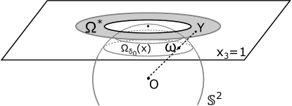
We have
is an annulus (or a disk) and
We define and use notation for the vector . If , then
| (10) |
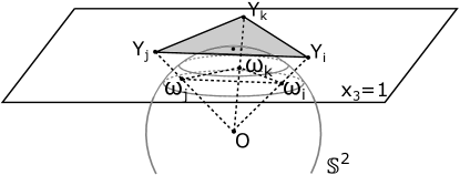
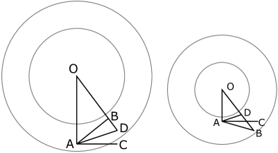
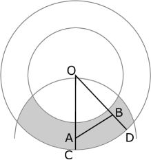
Since the distance of to the plane is , the volume of tetrahedron is one third of the area of triangle . Thus (please see figure 2)
We may combine this with (10) and obtain
| (11) |
Therefore we may use the reciprocal assumption on triples and , as well as the assumption to deduce (as long as is sufficiently small)
Here again the maximum is taken for all possible permutations of . We still call these two triangles and (weakly) reciprocal to each other and use the notation
We apply change of variables on the integral in (9), utilize (11) and obtain
In summary we have
Lemma 2.1.
Assume that with . Let be supported in the region . Then the function
satisfies the following inequality for all sufficiently small :
The constant is defined by
Here is an annulus (or disk) region in defined by
And consists of all (weakly) reciprocal triples of in :
Here the maximum is taken for all possible permutations of .
3 Geometric Observations
In this section we make some geometric observations. We first give a few geometric characteristics of (weakly) reciprocal triangles in and then a few properties an annulus region satisfies. Many of the following results are simple geometric observations and might have been previously known. Here we still give their proof for the reason of completeness. In this section we say that a triangle is of size if and only if .
3.1 Reciprocal triangles
In this subsection, we consider (weakly) reciprocal triangles in , as defined in the previous section.
Lemma 3.1.
Let be of size and satisfy . Then either or .
Proof.
We always have . Thus
∎
This immediately gives
Corollary 3.2.
Let be of size and satisfy . Then at least two of the following inequalities holds
Proposition 3.3.
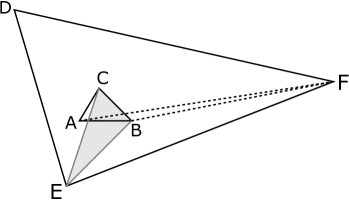
Let be reciprocal and of sizes , respectively. Then there exists a vertex of (say ) so that .
Proof.
Let us prove Proposition 3.3 by contradiction. We assume
Without loss of generality we also assume . Thus . We consider two cases: case 1, is close to the vertex ; case 2, is far away from the vertex .
Case 1
If . We apply Corollary 3.2 on and , at least two of the following holds
Similarly at least two of the following inequalities holds
Thus we may find two vertices from , say , so that we have
Next we show that either or holds. This immediately gives a contradiction to our reciprocal assumption. In fact, if the first inequality fails, i.e. , then we have
Our assumption guarantees that , thus we have
It immediately follows that . Thus
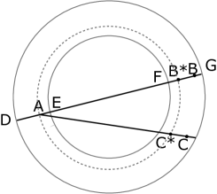
This finishes the argument in case one. Please see figure 3 for an illustration of the proof.

Case 2
In this case . Given any vertex , we have either or . As a result, we may find one vertex from (say ) and two vertices from (say ) so that
Combining these angles with our assumptions and , we obtain
| (12) |
Finally we apply Lemma 3.1 on and to conclude that either or holds. A combination of this with (12) immediately gives a contradiction. Please see figure 4 for an illustration of this case. Combining case 1 and 2, we finish the proof of Proposition 3.3. ∎
Corollary 3.4.
Let be reciprocal of sizes , respectively. Then they can not be too far away from each other. Namely we always have
Proof.
This corollary clearly holds if the size of one triangle is much larger than that of the other, thanks to Proposition 3.3. Thus we only need to consider the case . If the corollary failed, we would have
We may apply Corollary 3.2 on the triangle and the point , then on the same triangle and the point . This enable us to find two vertices from (say ) so that
We then apply Lemma 3.1 on the triangle and the point , then conclude that at least one of the following holds
Either of these contradicts our reciprocal assumption. ∎
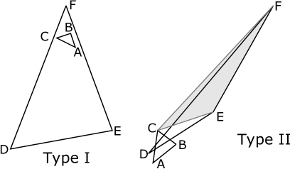
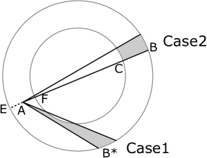
Proposition 3.5 (Classification).
Let and be two reciprocal triangles of sizes , respectively. Without loss of generality we also assume and are the shortest edge in the corresponding triangles. Then the location of smaller triangle satisfies either of the following
-
(I)
;
-
(IIa)
so that ;
-
(IIb)
so that .
We call these triangles Type I reciprocal if they satisfies (I) and call them Type II reciprocal if they satisfies either (IIa) or (IIb). Please see figure 5.
Proof.
Proposition 3.3 guarantees that if (I) fails, then we have either or . Without loss of generality, we assume and show that either (IIa) or (IIb) holds. Because , we may conclude that either or holds by considering the angles and . If the latter holds, satisfies (IIa). Thus we only need to consider the first case. Similarly we may assume . Now we claim that thus (IIb) holds. Otherwise we may apply Lemma 3.1 and conclude that either or . This means
thus contradicts the reciprocal assumption. ∎
3.2 About annulus
In this subsection we give a few geometric properties of a circular annulus region. We consider a circular annulus region , whose outer radius is , inner radius is and width is . We will also use the notation for the center of .
Lemma 3.6.
Assume and . Then
Proof.
First of all, if or , then the right hand side is greater or equal to , thus the inequality holds. We now assume thus . Let be the point on the ray so that . We have
We also have
Finally we have
∎
Corollary 3.7.
Assume and . Then
-
(a)
. Here is the terminal point of the vector in with starting point , length and direction .
-
(b)
If so that , then we have
Proof.
Let and , . By Lemma 3.6, we have
We observe ()
Thus the subset of consisting all possible directions of has a measure smaller or equal to . This proves part (a). For part (b), a similar argument shows
Thus
∎
Lemma 3.8.
Let so that . Then we have
Proof.
First of all, we claim that the line must intersect the inner boundary of at two different points, otherwise the length can never exceed . Let be the intersection points of the line with the boundary of , as shown in figure 7, so that is on the line segment . We have . In addition
This immediately gives . As a result, must be on the line segment . Let be the point on the line segment so that . We always have . We may define in a similar way, as shown in figure 7. Again we have . Since is on the same circle of radius , we have
Therefore
∎
Corollary 3.9.
Let so that . Then
-
(a)
;
-
(b)
.
Proof.
We may rewrite the conclusion of Lemma 3.8 in the form of
We then combine this inequality with the assumption
This proves part (a). Part (b) immediately follows part (a) and the basic formula
∎
Corollary 3.10.
Let so that . Then
Proof.
Lemma 3.11 (Area by angle).
Let and be measurable. Then
Proof.
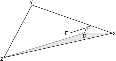
It suffices to consider the case . Here we slightly abuse the notation, the angle actually represent the direction . Let (or ) be the point where the ray meets the outer boundary of the annulus . We consider two cases. Case 1, if is relatively short, then we have
Case 2, if is long, then we claim that the segment must intersect with the inner boundary of at two different points. Otherwise the length can never exceed . Let be the intersection points of line with the boundary circles of , as shown in figure 8. We have
Thus we have ()
∎
Corollary 3.12.
Let , and . Then
Proof.
If , then the inequality is trivial since . If , then
We then utilize the inequality and apply Lemma 3.11 to complete the proof. ∎
Remark 3.13.
The following will also be used in the subsequent section: Assume , . Let be measurable. Then we have
Lemma 3.14 (Area by distance).
Let and . Then
Here is the disk of radius centered at .
Proof.
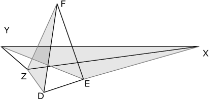
This is trivial if because in this case . Let us assume . Given any point , let be the intersection points of the rays , with the outer boundary of , as shown in figure 9. We have
Thus . This immediately gives
∎
4 Proof of Geometric Inequality
In this section we prove
Proposition 4.1.
Let be a circular annulus region with outer radius and width . Here . Then
Here is the set of all reciprocal triples of in , as defined in Lemma 2.1.
Remark 4.2.
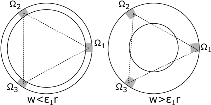
The upper bound given above is optimal. We choose three angles , , , and three regions accordingly by polar coordinates ( is a small constant)
as show in figure 10. If we choose triples , then and are reciprocal to each other, as long as the constant is sufficiently small. It is because these triangles are among the biggest triangles in the disk of radius . This implies if we fix , then
Sizes and angles
In order to take advantage of the geometric properties of reciprocal triangles, we sort all reciprocal triangles by their sizes and angles. We choose dyadic sequences of sizes:
We say that is of size if and only if . Without loss of generality we also assume that is the smallest among the three angles of . Thus we have . If is of size , then . As a result, we define (the upper bound of can be determined by Lemma 3.7)
and
We always have
| (13) |
We then sort all reciprocal triangles of a given triangle by their sizes and angles. We define
We immediately have for a fixed triangle
| (14) |
For convenience we also assume that the size of is and the smallest angle of is . We split the big sum in the right hand side into three parts: large sizes , small sizes and comparable sizes .
4.1 Large sizes
We first consider the case that the size of is much larger than that of . According to our classification of reciprocal triangles, we consider two cases, i.e. Type I reciprocal triangles and Type II reciprocal triangles. We write
Here
Type I
In this case we have . According to Lemma 3.1, we have either or . Without loss of generality let us assume the latter one.111Strictly speaking, we need to consider both two cases. The argument here only takes care of one case. The other case can be dealt with in exactly the same way. A combination of this and the reciprocal assumption implies
Thus we have
This means that if , then at least one of the following holds (see figure 11)
-
•
;
-
•
.
We may write as a union of two parts accordingly. Here we define
Now we are ready to find the upper bounds of the integrals ()
Let us first consider the case and . It is clear that
Next we give an upper bound of the measure of . First of all, we observe
Thus we may find an upper bound of the measure of instead. According to Lemma 3.14, the area of region is dominated by (up to a constant multiple). Furthermore, given such a point , we may apply Lemma 3.14 again and obtain that the area of the region is dominated by . Finally, given a pair as above, the area of the region is dominated by , thanks to Corollary 3.12. A product of the three upper bounds above gives the upper bound of . In summary we always have
Thus we have (In this case )
If , the case can be dealt with in the same way. We observe
We first choose an with , then determine the region containing all possible ’s by the angle , and finally determine the region of by the angle . This gives an upper bound
We may deal with the case in exactly the same way by using Remark 3.13, Lemma 3.14 and . The upper bounds are given by
We may combine all the upper bounds above and conclude
Type II
We may further write with
These two cases can be dealt with in exactly the same way. Let us consider the Type IIa reciprocal triangles, for instance. In this case
By our reciprocal assumption, we have (see figure 12)
That is
Canceling , and plugging , in, we have
Following the same argument as in the Type I case, we may write . Here we define
We then give upper bounds of the integrals below as in the Type I case: If , then
On the other hand, if , then
Finally we recall if and if , then take a sum for all and .
A similar inequality holds for Type IIb reciprocal triangles.
Summary
We may combine Type I and II cases and obtain that for any given , we have
Please note that the implicit constant in the inequality is an absolute constant, i.e. independent of .
4.2 Small sizes
We assume the size of is much smaller than that of , i.e. . Again we consider Type I and II reciprocal triangles separately. We define
Type I
By our reciprocal assumption we always have (please see figure 13)
Thus
Our assumption implies . Thus if , we have
Thus we have with

If , then we have (please note that , and )
If , then we have ()
Finally, if , then we have (; and )
Collecting the upper bounds above and taking a sum, we always have
Type II
Now we consider small, type II reciprocal triangles of a given triangle . This is the most difficult case. Let of size be a Type II reciprocal triangle of . Let us first give an upper bound of the integral
for given , . Without loss of generality, let us assume 222Strictly speaking, we need to consider four different cases. The argument given here only takes care of one from the four parts of . However, all these four cases can be dealt with in exactly the same way.
Thus by reciprocal assumption we immediately have
Since and , at least one of the following holds (see figure 14)
-
•
. By comparing the area of with that of we have
-
•
. By considering the area of we have .

Thus the region is the union of two parts:
If , we may find an upper bound of the integrals (, )
| (15) |
Similarly if , then we have ()
| (16) |
We may collect the upper bounds above and obtain
and
Thus it suffices to consider with and . We apply Lemma 3.8 and obtain
| (17) | ||||
| (18) |
Next we first prove
Lemma 4.3.
Let with . In addition, we assume . Then there exists an ansolute constant so that at least one of the following holds
-
(a)
;
-
(b)
and ;
-
(c)
and
Proof.
The proof consists of three steps.
Step 1
We first show that . Without loss of generality we assume and . If , then we would have
Since , we have either or . We consider these two cases separately. If , then our reciprocal assumption implies
According to Corollary 3.9, the inequality above implies
We cancel , recall the facts
and obtain . This is a contradiction. On the other hand, if , then we may follow a similar argument as above by considering , and obtain
This gives . Again this is a contradiction. As a result we obtain . It immediately follows that
Please refer to figure 15 for an illustration of the proof. Our remaining task is to show that if , then either (b) or (c) holds.

Step 2
Now we assume , there are two cases: are either both close to the point or both far away from . In this step we assume . Since we also have
We consider the triangles and . The reciprocal assumption immediately gives
Thus we may apply Corollary 3.10 and obtain
In other words, (b) holds. Please see the upper half of figure 16.

Step 3
Finally we assume and . This implies that . If we have
then our assumption on automatically guarantees (c) holds. Therefore we may additionally assume
Without loss of generality, we assume
We have
Thus , . We next apply Corollary 3.9 and obtain
The reciprocal assumption then gives
We then apply Corollary 3.9 again and conclude (please refer to lower half of figure 16)
Thus (c) holds. ∎
Completion of type II case
First of all, we recall that it suffices to consider with and . According to Lemma 4.3, the set of this kind is empty unless . Thus we may further assume . We recall the upper bounds given in (15), (16) and obtain
Therefore we only need to deal with with and . For convenience we use the notation . We recall (17), (18) and obtain that must satisfy and
According to Lemma 4.3, we may write
Here we define
We then apply Lemma 3.14, Corollary 3.12 and obtain ()
Thus
In summary we have
Summary
We may combine Type I and II cases and obtain that
4.3 Comparable Sizes
Finally let us the consider the case when and are about of the same size, i.e. . This eliminate the need to take a sum in . In this subsection we prove that if , then
The argument is similar to the case , Type II. Now we have less information on the relative location of two triangles available. Nevertheless, Corollary 3.4 guarantees that . By reciprocal assumption, we have (please refer to figure 17)
That is
Canceling , and plugging in, we have
Here the notation represents

Therefore we may write . Here
This immediately gives the upper bounds: if , then
If , then
In either case we may take a sum and obtain that if , then
4.4 Summary
Collecting all cases discussed above, we prove that the inequality
holds for all . The implicit constant here is an absolute constant. Thus we finish the proof of Proposition 4.1.
5 Applications of Geometric Inequalities
In this section we prove the main results given in Section 1.
5.1 Proof of Proposition 1.3
Part (a)
Let us temporally assume is supported in . We apply Proposition 4.1 and obtain an upper bound of defined in Proposition 2.1. (A disk of radius can be viewed as an annulus of outer radius and width )
Here
We plug and obtain that if , then (recall that and is small)
And if , then (in this case )
This upper bound of is an increasing function of in the interval and a decreasing function of in the interval . Thus we have
We plug this upper bound in Proposition 2.1, make and obtain
for all functions supported in and . Similarly we may choose , recall and obtain
By the identity
The same inequalities as above also hold for supported in . We then use the linearity of to finish the proof.
Part (b)
Now let us assume is supported in . We may break into pieces
so that
It immediately gives a convergence in :
We then apply the conclusion of part (a) on the radiation profiles and obtain
Therefore
This finishes the proof of part (b).
5.2 Proof of Corollary 1.4
Since we always have , we may assume , without loss of generality. Let thus we have . There are two cases
5.3 Proof of Proposition 1.6
The estimates
Let be the radiation profile associated to the linear free wave . By isometric property we have . The non-radiative assumption implies that is supported in . We may define and rewrite
We have
We then apply Corollary 1.4 and obtain
Therefore we have
The decay immediately follows Proposition 1.3, part (a), as long as
The case is trivial.
The estimates
We recall the Strichartz estimates given in Ginibre-Velo [12]: if satisfies and , then any finite-energy linear free wave satisfies
| (19) |
As a result, the decay of the norm follows an interpolation between the decay estimate
and the regular Strichartz estimate (19) with and in the whole space. Please note that the choice is forbidden in the Strichartz estimates.
6 Two dimensional case and application on Radon transform
Since is the adjoint operator of Radon transform , a corollary immediately follows Proposition 1.3: If is supported in the region , then
We are also interested in its 2-dimensional analogue, since 2-dimensional Radon transform is more frequently used in some applications, for example, X-ray technology. Our 2-dimensional result is
Proposition 6.1.
We consider the 2-dimensional Radon transform ( is the line measure of a straight line on )
and its adjoint
Then we have
-
(a)
Assume that with . If is supported in , then
-
(b)
Assume that . If is supported in , then
-
(c)
If for all , then we have
Proof.
The general idea is exactly the same as in the 3-dimensional case. Part (b) follows part (a) and a decomposition of . Part (c) follows a basic property of adjoint operators. Let us stretch the proof of part (a) only. Following the same argument as in Section 2, we obtain ( is sufficiently small)
Here the constant is defined by
Here is defined by
and is the set consisting of reciprocal pairs of . We call and are reciprocal pairs if and only if
We claim that if with , then
| (20) |
We then plug this upper bound in the expression of , take the least upper bound, then make to finish the proof of part (a). Finally we need to verify (20). First of all, if and are reciprocal pairs, then we claim
| (21) |
In fact, we may assume without loss of generality. The triangle inequality implies that we have either or . By our reciprocal assumption we have either or . This verifies (21). Now we are ready to prove (20). Let us fix . We define to be the set of all reciprocal pairs of size :
We also assume that the size of is , i.e. so that . There are two cases: Case 1, if , then we must have either or . In addition (21) implies that if , then either or holds, thus . This implies
Case 2, if , then we have either or by (21), thus . (Please note that ) Therefore we have
In summary
This finishes the proof. ∎
Acknowledgement
The authors are financially supported by National Natural Science Foundation of China Project 12071339.
References
- [1] R. Côte, and C. Laurent. “Concentration close to the cone for linear waves.” arXiv preprint 2109.08434.
- [2] R. Côte, C.E. Kenig and W. Schlag. “Energy partition for linear radial wave equation.” Mathematische Annalen 358, 3-4(2014): 573-607.
- [3] T. Duyckaerts, C.E. Kenig, and F. Merle. “Universality of blow-up profile for small radial type II blow-up solutions of the energy-critical wave equation.” The Journal of the European Mathematical Society 13, Issue 3(2011): 533-599.
- [4] T. Duyckaerts, C.E. Kenig, and F. Merle. “Classification of radial solutions of the focusing, energy-critical wave equation.” Cambridge Journal of Mathematics 1(2013): 75-144.
- [5] T. Duyckaerts, C.E. Kenig, and F. Merle. “Scattering for radial, bounded solutions of focusing supercritical wave equations.” International Mathematics Research Notices 2014: 224-258.
- [6] T. Duyckaerts, C.E. Kenig, and F. Merle. “Scattering profile for global solutions of the energy-critical wave equation.” Journal of European Mathematical Society 21 (2019): 2117-2162.
- [7] T. Duyckaerts, C. E. Kenig, and F. Merle. “Decay estimates for nonradiative solutions of the energy-critical focusing wave equation.” arXiv preprint 1912.07655.
- [8] T. Duyckaerts, C. E. Kenig, and F. Merle. “Soliton resolution for the critical wave equation with radial data in odd space dimensions.” arXiv preprint 1912.07664.
- [9] F. G. Friedlander. “On the radiation field of pulse solutions of the wave equation.” Proceeding of the Royal Society Series A 269 (1962): 53-65.
- [10] F. G. Friedlander. “An inverse problem for radiation fields.” Proceeding of the London Mathematical Society 27, no 3(1973): 551-576.
- [11] F. G. Friedlander. “Radiation fields and hyperbolic scattering theory.” Mathematical Proceedings of Cambridge Philosophical Society 88(1980): 483-515.
- [12] J. Ginibre, and G. Velo. “Generalized Strichartz inequality for the wave equation.” Journal of Functional Analysis 133(1995): 50-68.
- [13] S. Helgason. “The Radon transform on Euclidean spaces, compact two-point homogeneous spaces and Grassmann Manifolds.” Acta Mathematica 113(1965): 153-180.
- [14] S. Helgason. The Radon Transform, second edition, Birkhäuser 1999, Boston, Massachusetts, USA.
- [15] C. E. Kenig, A. Lawrie, B. Liu and W. Schlag. “Relaxation of wave maps exterior to a ball to harmonic maps for all data” Geometric and Functional Analysis 24(2014): 610-647.
- [16] L. Li, R. Shen and L. Wei. “Explicit formula of radiation fields of free waves with applications on channel of energy”, arXiv preprint 2106.13396.
- [17] D. Ludwig. “The Radon transform on Euclidean space.” Communications on Pure and Applied Mathematics 19, no. 1(1966): 49-81.
- [18] R. Shen. “On the energy subcritical, nonlinear wave equation in with radial data” Analysis and PDE 6(2013): 1929-1987.