Swiss-cheese cosmologies with variable $G$ and $\Lambda$ from the renormalization group

Abstract

A convincing explanation for the nature of the dark energy and dark matter is still missing. In recent works a RG-improved swiss-cheese cosmology with an evolving cosmological constant dependent on the Schücking radius has been proven to be a promising model to explain the observed cosmic acceleration. In this work we extend this model to consider the combined scaling of the Newton constant $G$ and the cosmological constant $\Lambda$ according to the IR-fixed point hypothesis. We shall show that our model easily generates the observed recent passage from deceleration to acceleration without need of extra energy scales, exotic fields or fine tuning. In order to check the generality of the concept, two different scaling relations have been analysed and we proved that both are in very good agreement with $\Lambda$CDM cosmology. We also show that our model satisfies the observational local constraints on $\dot{G}/G$.

I Introduction

Although the $\Lambda$CDM scenario reproduces rather well a large amount of observational data, it is important to stress that its two main ingredients, Dark Matter (DM) Rubin and Ford (1970) and Dark Energy (DE) Spergel et al. (2007), do not have a direct physical explanation. In particular, the observed accelerated expansion of the Universe is caused by the DE component a mechanism which introduces new difficulties in terms of fine-tuning or cosmic coincidences Straumann (1999) for the presence of a significant vacuum energy (cosmological constant).

For this reason the possibility that the cosmological constant is dynamically generated as a low-energy quantum effect has been recently investigated by various authors Wang et al. (2017); Carlip (2019). In particular in Bonanno and Reuter (2002) a cosmology with a time dependent cosmological constant and Newton constant whose dynamics arises from an underlying renormalization group flow near an infrared attractive fixed point has been proposed for the first time. Its phenomenological implications have been discussed in Bentivegna et al. (2004) and further developed in Bonanno and Carloni (2012).

The IR-fixed point hypothesis originates from the asymptotically safe (AS) scenario for quantum gravity Weinberg (1979); Reuter (1998). According to AS a consistent quantum theory of gravity can be realized nonperturbatively by defining the theory around a non-gaussian fixed point for the dimensionless Newton’s constant Litim (2011); Nagy (2014); Bonanno and Saueressig (2017); Percacci (2017); Eichhorn (2019); Pereira (2019); Reuter and Saueressig (2019); Reichert (2020); Platania (2020). In fact this mechanism is not qualitatively different from what occurs in the non-linear $\sigma$-model in $d=3$: here too, although the theory is not perturbatively renormalizable, a continuum limit at non-vanishing value of the coupling constant can be defined beyond perturbation theory Polyakov (1993); Codello and Percacci (2009).

Assuming that the relevant scale of energy or momentum scales with the distance as the coarse-graining, “resolution” scale of the renormalization group, the spatial or temporal evolution of the Newton’s constant and cosmological constant is dictated by the renomalization group flow Platania (2020). The possibility of explaining DM in spiral galaxies as an infrared effect of the running of $G$ has been discussed in Reuter and Weyer (2004a, b), while complete cosmological histories based on RG-trajectories emanating from the UV fixed point up to the IR regime have been discussed in Reuter and Saueressig (2005); Bonanno and Reuter (2007). Non-singular cosmological models have appeared in Kofinas and Zarikas (2016); Bonanno et al. (2018) and a mathematical formalism to couple the RG evolution to the Einstein equations have been discussed in Reuter and Weyer (2004) and Bonanno et al. (2021).

In Kofinas and Zarikas (2018) a further step in the direction of explaining the DE content in the Universe with a running cosmological constant has been proposed. The basic idea is to consider the contribution of an homogeneous distribution of antigravity sources associated with the matter content at galactic and cluster scale. A swiss-cheese cosmology represents an elegant mathematical framework to implement this idea which has been elaborated also in Mitra et al. (2021); Anagnostopoulos et al. (2019a, b). In this work we would like to extend the original RG-improved swiss-cheese model to include the running of the Newton’s constant according to the IR-fixed point mechanism. In this case, the scaling behavior of $G$ and $\Lambda$ is determined by the simple law

$$G_{k}\equiv G(k)\sim g_{\ast}/k^{2},\quad\quad\Lambda_{k}\equiv\Lambda(k)\sim\lambda_{\ast}k^{2}$$ (1)

in the $k\rightarrow 0$ limit. This behavior could be the result of a “tree-level” renormalization induced by a non-zero positive cosmological constant in the IR, according to the singular behavior of the $\beta$-functions in the IR Nagy et al. (2012); Christiansen et al. (2014); Biemans et al. (2017). The aim of this study is to further elaborate the IR-fixed point scaling within the swiss-cheese cosmology. In particular it will be shown that it is possible to consistently describe a phase of accelerated expansion of the universe without the introduction of a DE component.

The structure of this paper is the following: in section II the mathematical the swiss-cheese idea and the basic equations will be discussed. In Section III the IR fixed point hypothesis and the RG evolution will be presented as a function of the Schücking Radius and of the matter density. In section IV the numerical results are discussed and section V is devoted to the conclusions.

II Swiss cheese cosmological model

The original Einstein-Strauss model or otherwise called swiss-cheese model, Einstein and Straus (1946), describes many homogeneously distributed black holes smoothly matched within a cosmological metric. The key idea is to match a Schwarzshild spherical vacuole in a homogeneous isotropic cosmological spacetime. The analysis finally generates a dust Friedman-Robertson-Walker (FRW) cosmology assuming many Schwarzschild black holes as the matter content.

It is also possible to show that respecting the Israel-Darmois matching conditions, Eisenhart (2016), a homogeneous and isotropic cosmological metric with a de Sitter - Schwarzschild like metric can be successfully matched across a spherical 3-surface $\Sigma$ which is at fixed coordinate radius of the cosmology metric frame (see also Balbinot et al. (1988)). However, the radius of the surface in the Black Hole (BH) frame is time evolving. The matching requires the first fundamental form, intrinsic metric, and second fundamental form (extrinsic curvature), calculated in terms of the coordinates on $\Sigma$, to be equal (opposite for the second fundamental form) on both sides of the surface Darmois (1927), Dyer and Oliwa (2000).

A homogeneous isotropic cosmological metric can be written in spherical coordinates as

$$ds^{2}=-dt^{2}+a^{2}(t)\left[r^{2}\left(d\theta^{2}+\sin^{2}\theta\,d\phi^{2}\right)+(1-\kappa\,r^{2})^{-1}\,dr^{2}\right]\,,$$ (2)

where $a(t)$ is the scale factor and $\kappa=0,\pm 1$ is the spatial curvature constant.

The junction conditions Eisenhart (2016) allow us to use different coordinate systems on both sides of the hypersurface. Thus, the cosmology exterior metric (2) can be joined smoothly to the following quantum-modified Schwarzschild metric,Koch and Saueressig (2014),

$$ds^{2}=-F(R)\,dT^{2}+R^{2}\left(d\theta^{2}+\sin^{2}\theta d\phi^{2}\right)+F(R)^{-1}\,dR^{2}\,$$ (3)

where F(R) is defined by

$$F\left(R\right)=1-\frac{2\,G_{k}\,M}{R}-\frac{\Lambda_{k}\,R^{2}}{3}.$$ (4)

Note, that now the Newton constant and the cosmological constants are not constants but functions of one characteristic length scale $\sim 1/k$. Both will be functions of $R$ as we shall explain later. The first fundamental form is the metric on $\Sigma$ induced by the spacetime in which it is embedded. This may be written as

$$\gamma_{\alpha\beta}=g_{ij}\frac{\partial}{\partial u^{\alpha}}x^{i}\frac{\partial}{\partial u^{\beta}}x^{i}\,,$$ (5)

where $u^{\alpha}=(u^{1}\equiv u,\,u^{2}\equiv v,\,u^{3}\equiv w)$ is the coordinate system on the hypersurface. Greek indices run over $1,\ldots,3,$ while Latin indices over $1,\ldots,4.$
The second fundamental form Eisenhart (2016) is defined by

$$K_{\alpha\beta}=n_{i;j}\,\frac{\partial}{\partial u^{\alpha}}x^{i}\frac{\partial}{\partial u^{\beta}}x^{i}=(\Gamma^{p}{}_{ij}n_{p}-n_{i,j})\frac{\gamma_{\alpha\beta}}{g_{ij}}\,,$$ (6)

where $n_{a}$ is a unit normal to $\Sigma$ and $\Gamma^{p}{}_{ij}$ are the Christoffel symbols. We use subscripts $F$ and $S$ to denote quantities associated with the FLRW and modified Schwarzschild metrics, respectively Dyer and Oliwa (2000).

Let us consider a spherical hypersurface $\Sigma$ given by the function $f_{F}(x_{F}^{i})=r-r_{\Sigma}=0,$ where $r_{\Sigma}$ is a constant. This hypersurface in the FLRW frame can be parametrized by $x_{F}^{i}\,=\,(t=u,\,\theta=v,\,\phi=w,\,r=r_{\Sigma})$, while the parametrization in the BH frame is $x_{S}^{i}=\left(T=T_{S}(u),\,\theta=v,\,\phi=w,\,R=R_{S}(u)\right)$. The fact that we model $R=R_{S}(u)$ implies that the hypersurface $\Sigma$ may not remain in constant BH radial distance as the universe expands. This radial distance is also called Schücking radius. The successful matching will prove that this choice of the matching surface was the appropriate thing to do for successful modeling of the junction. From now on wherever in this section we write $T$ and $R$ we mean $T_{S}$ and $R_{S}$ respectively. The first Darmois condition $\gamma_{F\alpha\beta}=\gamma_{S\alpha\beta}$ gives

$$-1=-F(R)\,\left(\frac{dT}{du}\right)^{2}+F(R)^{-1}\left(\frac{dR}{du}\right)^{2}\,,$$ (7)

and

$$a^{2}\,r_{\Sigma}^{2}=R^{2}\,.$$ (8)

where as we have explained, $R=R_{S}$. The last equation 8 is an important one and describes that the matching takes place in the hypersurface $\Sigma$ where the BH radial distance is the time dependent Schücking radius $R_{S}$ and the cosmological coordinate distance is the constant $r=r_{\Sigma}$.

The second Darmois condition requires to estimate the two second fundamental forms. First the normal vector ,$n_{i}$, to the spherical hypersurface $\Sigma$ has to be evaluated. If $\Sigma$ is given by the function $f[x^{a}(u^{\alpha})]=0$, then $n_{i}$ can be calculated from

$$n_{i}=-\frac{f_{,i}}{\sqrt{|g^{ab}f_{,a}f_{,b}|}}\,,$$ (9)

where $,i$ denotes $\frac{\partial}{\partial x^{i}}$ .

The (outward pointing) unit normal in the FLRW frame can be calculated from Eq. (9) and $f_{F}(x_{F}^{i})=r-r_{\Sigma}=0.$ The result is

$$n_{Fi}=(0,0,0,-(\frac{a^{2}}{1-k\,r_{\Sigma}})^{1/2}).$$ (10)

Note, that the unit normal is spacelike, i.e. $n_{F}^{i}n_{Fi}=+1$. Since the equation of the matching surface $f_{F}(x_{S}^{i})$ is uknown in the Schwarzschild frame the normal vector $n_{S}^{i}$ cannot be calculated directly from Eq. (9). A condition for $n_{S}^{i}$ can be derived from the partial differentiation of $x_{S}^{i}(u^{\alpha})$ with respect to $u^{\alpha}$ which generates a tangential vector to the hypersurface $\Sigma$.

$$n_{Si}\frac{\partial x_{S}^{i}}{\partial u^{\alpha}}=0\,,$$ (11)

From (11) one obtains $n_{S2}=n_{S3}=0$ and

$$n_{S1}\frac{dT}{du}+n_{S4}\frac{dR}{du}=0.$$ (12)

Furthermore, $n_{S}^{i}$ must satisfy the identity

$$n_{S}^{i}n_{Si}\equiv n_{F}^{i}n_{Fi}=1\;\;$$ (13)

Then (13) gives

$$-\left(F(R)\right)^{-1}{n_{S1}}^{2}+F(R){n_{S4}}^{2}=1.$$ (14)

Now using equation (7) and equations (14), (12) it is possible to evaluate $n_{Si}$ as a function of $u^{\alpha}:$

$$n_{Si}=\left(\mp\frac{dR}{du},\;0,\;0,\;\pm\frac{dT}{du}\right)\,.$$ (15)

The second fundamental form can be easily calculated in the FLRW frame due to the simple form of $n_{Fi},$ Eq. (10). Thus from (6) we get

$$K_{F\alpha\beta} = \Gamma^{4}_{Fij}n_{F4}\frac{\partial x^{i}_{F}}{\partial u^{\alpha}}\frac{\partial x^{j}_{F}}{\partial u^{\beta}}-n_{F4,j}\frac{\partial x^{4}_{F}}{\partial u^{\alpha}}\frac{\partial x^{j}_{F}}{\partial u^{\beta}}$$ (16)

However, $\frac{\partial x^{4}_{F}}{\partial u^{\alpha}}=\frac{\partial r_{\Sigma}}{\partial u^{\alpha}}=0$, and

$$\frac{\partial x^{i}_{F}}{\partial u^{\alpha}}\frac{\partial x^{j}_{F}}{\partial u^{\beta}}=\frac{\partial x^{\mu}_{F}}{\partial u^{\alpha}}\frac{\partial x^{\nu}_{F}}{\partial u^{\beta}}=\delta^{\mu}_{\alpha}\delta^{\nu}_{\beta}$$ (17)

so the second fundamental form becomes

$$K_{F\alpha\beta} = n_{F4}\Gamma^{4}_{F\alpha\beta}$$ (18)

$$= -\frac{1}{2}|g_{F44}|^{1/2}g_{F}^{4i}(g_{F\alpha i,\beta}+g_{F\beta i,\alpha}-g_{F\alpha\beta,i})$$

$$= \frac{1}{2}|g_{F44}|^{1/2}g_{F}^{44}g_{F\alpha\beta,4}\,,$$

and finally

$$K_{F\alpha\beta}=\frac{1}{2}\left(\frac{a^{2}}{1-\kappa\,r^{2}}\right)^{-{1/2}}g_{F\alpha\beta,4}\,.$$ (19)

From equation (19) it is obvious that the only non zero components of $K_{F\alpha\beta}$ are $K_{F22}$ and $K_{F33}$

The estimation of the second fundamental form of $\Sigma$ in the Schwarzschild frame is more complicated. First we have to calculate $n_{Si}$ as a function of $x_{S}^{i}.$ If we once more differentiate Eq. (11) with respect to $u^{\alpha}$ it follows that

$$n_{Si,j}\frac{\partial x_{S}^{i}}{\partial u^{\alpha}}\frac{\partial x_{S}^{j}}{\partial u^{\beta}}=-n_{Si}\frac{\partial^{2}x_{S}^{i}}{\partial u^{\alpha}\partial u^{\beta}}\,,$$ (20)

which with the help of the definition equation 6, gives

$$K_{S\alpha\beta}=\Gamma^{p}_{Sij}n_{Sp}\frac{\partial x_{S}^{i}}{\partial u^{\alpha}}\frac{\partial x_{S}^{j}}{\partial u^{\beta}}+n_{Si}\frac{\partial^{2}x_{S}^{i}}{\partial u^{\alpha}\partial u^{\beta}}\,.$$ (21)

Using equation (21), we find that $K_{S\alpha\beta}=0,\,\forall\,\alpha\neq\beta.$ This is true since the second derivative is zero for $\alpha\neq\beta$ and the first term of equation (21) also is zero for $\alpha\neq\beta$ due to the specific Christoffel symbols.

The second Darmois matching condition $K_{S\alpha\beta}=K_{F\alpha\beta}$ on $\Sigma,$ provides the following differential equations

$$K_{S11} \equiv \Gamma^{4}_{S11}n_{S4}\left(\frac{dT}{du}\right)^{2}+\Gamma^{4}_{S44}n_{S4}\left(\frac{dR}{du}\right)^{2}+2\Gamma^{1}_{S14}n_{S1}\frac{dT}{du}\frac{dR}{du}$$ (22)

$$\ +n_{S1}\frac{d^{2}T}{du^{2}}+n_{S4}\frac{d^{2}R}{du^{2}}=0\equiv K_{F11}\,,$$

since $p$ can be either 1 or 4 for non zero $n_{Sp}$ and the only relevant non zero Christofell symbols $\Gamma^{1}_{Sij}$, $\Gamma^{4}_{Sij}$ are only $\Gamma^{1}_{S14},\,\Gamma^{1}_{S41}$ and all $\Gamma^{4}_{Sii}$. It is also

$$K_{S22}=K_{F22}\Leftrightarrow\Gamma^{4}_{S22}n_{S4}=a\,r_{\Sigma}\sqrt{1-\kappa\,r_{\Sigma}^{2}}$$ (23)

and

$$K_{S33}=K_{F33}\Leftrightarrow\Gamma^{4}_{S33}n_{S4}=a\,r_{\Sigma}\sin^{2}\theta\,\sqrt{1-\kappa\,r_{\Sigma}^{2}}\,.$$ (24)

Now the relevant Christoffel symbols are $\Gamma^{1}_{S14}=\frac{F^{\prime}}{2F},\,\,\Gamma^{4}_{S44}=-\frac{F^{\prime}}{2F},\,\,\Gamma^{4}_{S11}=\frac{1}{2}F\left(F^{\prime}\right),\,\,\Gamma^{4}_{S22}=-R\,F,\,\,\Gamma^{4}_{S33}=-\sin^{2}\theta\,R\,F,\,$ where notation ”^′” is understood as derivative with respect to $R$.

Equations (23) and (24) being equivalent, we can use either of them and Eq. (8) to obtain

$$\frac{dT}{du}=\mp\frac{\sqrt{1-\kappa\,r_{\Sigma}^{2}}}{1-\frac{2\,G_{k}\,M}{R}-\frac{\Lambda_{k}\,R^{2}}{3}}\,.$$ (25)

It then follows from Eq. (7) that

$$\left(\frac{dR}{du}\right)^{2}=\frac{2\,G_{k}\,M}{R}+\frac{\Lambda_{k}\,R^{2}}{3}-\kappa\,r_{\Sigma}^{2}\,.$$ (26)

Now differentiating eqs. (25) and (26) w.r.t. to $u$, we get the following expressions

$$\frac{d^{2}T}{du^{2}}=\pm\sqrt{1-\kappa\,r_{\Sigma}^{2}}\,\frac{d\Big{(}+\frac{2G_{k}M}{R}+\frac{1}{3}\Lambda_{k}R^{2}\Big{)}}{dR}\,\Big{(}1-\frac{2G_{k}M}{R}-\frac{1}{3}\Lambda_{k}R^{2}\Big{)}^{-2}\,\frac{dR}{du}\,.$$ (27)

and

$$\frac{d^{2}R}{du^{2}}=\frac{1}{2}\,\frac{d\Big{(}\frac{2G_{k}M}{R}+\frac{1}{3}\Lambda_{k}R^{2}\Big{)}}{dR}$$ (28)

With equations (25)-(28), Eq. (22) is now identically satisfied. Thus, both the first and second fundamental forms are continuous on $\Sigma$.

Note that the cosmic evolution through the swiss-cheese is determined by the cosmic evolution of the matching surface that is happening at spherical radius, in the black hole frame, $R_{S}$ (and constant $r_{\Sigma}$ for cosmic frame). This quantity enters the differential equations.

Finally, the matching requirements provide the following equations that are relevant for the cosmological evolution. From this point and to the rest of the paper we use again separately the symbol $R$ for the BH radial distance and the symbol $R_{S}$ for the Shucking radius,

$$R_{S} = ar_{\Sigma}$$ (29)

$$\Big{(}\frac{dR_{S}}{dt}\Big{)}^{2} = 1\!-\!\kappa r_{\Sigma}^{2}-\Big{(}1-\frac{2G_{k}(R_{S})\,M}{R_{S}}-\frac{1}{3}\Lambda_{k}(R_{S})\,R_{S}^{2}\Big{)}$$ (30)

$$2\frac{d^{2}R_{S}}{dt^{2}} = \frac{d\Big{(}\frac{2G_{k}(R)\,M}{R}+\frac{1}{3}\Lambda_{k}(R)\,R^{2}\Big{)}}{dR}|_{R_{S}}$$ (31)

The matching radius $r_{\Sigma}$ can be also understood as the boundary of the volume of the interior solid with energy density equal to the cosmic matter density $\rho$. Thus, the interior energy content should equal the mass $M$ of the astrophysical object, i.e.

$$r_{\Sigma}=\frac{1}{a_{0}}\Big{(}\frac{2G_{\!N}M}{\Omega_{m0}H_{0}^{2}}\Big{)}^{\!\frac{1}{3}}\,,$$ (32)

with density parameter $\Omega_{m}=\frac{8\pi G_{\!N}\rho}{3H^{2}}=\frac{2G_{\!N}M}{r_{\Sigma}^{3}a^{3}H^{2}}$ and $a_{0}$ set to be 1 for the rest of the analysis.

A rather important information in the context of the aforementioned approach is the exact physical element of our model, galaxies, clusters of galaxies or even super-clusters. In order to answer this, we should look at the physical interpretation of the Schücking radius, $r_{\Sigma}$, and its relation with measurable scales of the above astrophysical objects. For Milky Way ($M_{MW}\sim 4\cdot 10^{11}\ M_{\odot}$) with typical values of cosmological parameters ($\Omega_{m0}\sim 0.3,\ H_{0}\sim 67$ km/Mpc/s, Planck Collaboration et al. (2020)) using Eq.((32)) we have $r_{\Sigma}\sim 1.4$ Mpc where the astrophysical radius is $R_{as}\sim 0.15$ Mpc. Similarly, for the Local Group $M_{LG}\sim(7-20)\cdot 10^{11}$ we find $r_{\Sigma}\sim 2.34$Mpc and the astrophysical radius is $R_{as}\sim 1.53$ Mpc. Lastly, for the case of our local super-cluster, VIRGO ($M_{VSC}\sim 10^{15}\ M_{\odot}$) it is $R_{as}\sim 30.67$ Mpc and $r_{\Sigma}\sim 4$ Mpc. We observe that only in the scale of galaxy clusters it is $r_{\Sigma}/R_{as}$ of order $\mathcal{O}(1)$, thus thereafter we will consider galaxy clusters as the elementary entities of the model.

Eqs. (29, 30, 31) for constant $G_{k}$ and $\Lambda_{k}$ reduce to the conventional Friedman-Lemaitre-Robertson-Walker (FLRW) expansion equations. However, although these equations generate the standard cosmological equations of the $\Lambda\text{CDM}$ model, even in this simple case the interpretation is different since the $\Lambda$ term appearing in the black hole metric, Koch and Saueressig (2014), is like an average of all anti-gravity sources inside the Schücking radius of a galaxy or cluster of galaxies. These anti-gravity sources one can claim that may arise inside astrophysical black holes in the centers of which the presence of a quantum repulsive pressure could balance the attraction of gravity to avoid the not desired singularity, or they arise due to IR quantum corrections of a concrete quantum gravity theory. Furthermore, even for constant $G_{k}$ and $\Lambda_{k}$ the coincidence problem can be removed if the anti-gravity sources, due to the local effective positive cosmological constant, are related with the large scale structure that appears recently. In our analysis, we allow the running of $G_{k}$ and $\Lambda_{k}$ which is the most natural thing if there are IR quantum gravity corrections.

III IR fixed point and cosmic acceleration

In this section the basic idea of the IR fixed point RG scaling will be introduced and the cosmic evolution of this model will be discussed.

III.1 The IR fixed point scaling

The presence of an IR instability in the RG flow for $G$ and $\Lambda$ is deeply rooted in the structure of the fluctuations determinant associated to the Einstein-Hilbert action

$$S_{k}=\frac{1}{16\pi G_{k}}\int dx^{4}\sqrt{g}(-\mathcal{R}+2\Lambda_{k}).$$ (33)

Let us consider a family of off-shell spherically symmetric contributions labelled by the radius $\phi$ in order to distinguish the contributions from the two operators $\sqrt{g}\propto\phi^{4}$ and $\sqrt{g}\mathcal{R}\propto\phi^{2}$ to the Einstein-Hilbert flow Reuter and Weyer (2004b). It is possible to decompose the fluctuating metric $h_{\mu\nu}$ to the sphere into its irreducible pieces in terms of the corresponding spherical harmonics. In particular, in the transverse-traceless sector the operator $S^{(2)}_{k}$ is given by

$$-g^{\mu\nu}\nabla_{\mu}\nabla_{n}u+8\phi^{-2}+k^{2}-2\Lambda_{k}$$ (34)

up to a positive constant. If the spectrum of the covariant laplacian $-g^{\mu\nu}\nabla_{\mu}\nabla_{n}u$ is non-negative, a singularity develops at a finite $k$ in the case of a positive cosmological constant.

In a scalar field theory an identical mechanism is present when the hessian of the action vanishes in the broken phase. In this case perturbation theory fails and the path-integral is dominated by non-homogeneous configurations Ringwald and Wetterich (1990) that produces a “tree-level” instability renormalization already at level of the bare action Alexandre et al. (1999). In spite of the complexity of the vacuum structure, the approach based on functional flow equation is able to sum an infinite tower of (irrelevant UV) operator and it reproduces the correct flattening of the effective potential $U(\phi)$ in the broken phase Bonanno and Lacagnina (2004). In this case, below the coexistence line, the potential behaves as $U(\phi)\propto-k^{2}\phi^{2}$ and approaches a flat bottom as $k\rightarrow 0$ Berges et al. (2002).

In gravity the situation is more difficult because of the technical difficulties in solving the RG flow equation beyond the Einstein-Hilbert truncation in the $k\rightarrow 0$ limit Benedetti and Caravelli (2012); Demmel et al. (2014); Dietz and Morris (2013). Based on the analogy with the scalar theory one can imagine that a RG trajectory which realizes a tree-level renormalization exists Ohta and Yamada (2021). In particular one can write that in the $k\rightarrow 0$ limit the dimensionless Newton constant and cosmological constant are attracted toward an IR fixed point $(g_{*},\lambda_{*}$) according to the following trajectory

$$g\left(k\right)=g_{*}+h_{1}k^{\theta_{1}},\quad\quad\lambda\left(k\right)=\ \lambda_{*}+h_{2}k^{\theta_{2}},$$ (35)

where $(\theta_{1},\theta_{2}\geq 0)$ are two unknown critical exponents. In terms of dimensionful quantities, we thus have

$${G(k)}_{{IR}}=\frac{g_{*}}{k^{2}}+h_{1}k^{\theta_{1}-2}\quad\quad\Lambda\left(k\right)_{{IR}}=\ \lambda_{*}k^{2}+h_{2}k^{\theta_{2}+2}$$ (36)

Here, $k$ should be considered not as a momentum flowing into a loop, but as an inverse of a characteristic distance, of the physical system under consideration, over which the averaging of the field variables is performed. It can then be associated to the radial proper distance or the matter density. F

For the rest of the paper in order to study the late cosmic evolution, we assume that the values of Newton constant and cosmological constant at the astrophysical scales will be those suggested in Eq. (36) i.e. $G_{k}={G(k)}_{{IR}}$ and $\Lambda_{k}=\Lambda\left(k\right)_{{IR}}$ .

In the first case we need to calculate the radial proper distance and in particular the Schücking proper radial distance, $D_{p}(R_{S})$, which can be found from

$$D_{p}\left(R_{S}\right)=\ \int_{R_{min}}^{R_{S}}\frac{R}{\sqrt{F(R)}}$$ (37)

where $R_{min}$ is zero in our case or a very small value if AS provides a non singular black hole center, see Aliferis and Zarikas (2021). Then, the derivative with respect to $R$ is

$$D_{p}^{{}^{\prime}}\left(R_{S}\right)=\ \frac{1}{\sqrt{F(R_{S})}}$$ (38)

Next, from matching equations equations (29,30,31) we get

$${\left(\frac{dR_{S}}{dt}\right)}^{2}=1-\kappa\,r_{\Sigma}^{2}-F(R_{S})$$ (39)

which gives

$$r_{\Sigma}^{2}{\dot{a}}^{2}=1-\kappa\,r_{\Sigma}^{2}-1+\frac{2\,G_{k}(R_{S})\,M}{R_{S}}+\frac{1}{3}\Lambda_{k}(R_{S})\,R_{S}^{2}$$ (40)

and

$$\frac{{\dot{a}}^{2}}{a^{2}}=-\frac{\kappa}{a^{2}}+\frac{2G_{k}(R_{S})M}{a^{3}\,r_{\Sigma}^{3}}+\frac{1}{3}\Lambda(R_{S})$$ (41)

III.2 Scaling using the Cluster Radial proper distance

Here the scaling we assume uses the proper distance

$$k=\frac{\xi}{D_{p}(z)}$$ (42)

Using Eq.(41) we get

$$\frac{{\dot{a}}^{2}}{a^{2}}+k\frac{1}{a^{2}}=\chi+\psi$$ (43)

where

$$\chi=2\left[\frac{g_{*}}{\xi^{2}}D_{p}^{2}+h_{1}\xi^{\theta_{1}-2}D_{p}^{2-\theta_{1}}\right]M\frac{1}{r_{\Sigma}^{3}a^{3}}$$ (44)

and

$$\psi=\frac{1}{3}\left[\lambda_{*}\xi^{2}D_{p}^{-2}+h_{2}\xi^{\theta_{2}+2}D_{p}^{-2-\theta_{2}}\right].$$ (45)

One useful quantity for evaluating the dark energy is the rate of change of the proper Shucking distance $D_{p}$. We have $\frac{dD_{p}}{\text{dR}}=\frac{dD_{p}}{\text{dt}}\frac{\text{dt}}{\text{dR}}=\frac{1}{\sqrt{F(R_{S})}}$ and thus,

$$\frac{dD_{p}}{dz}=\frac{-r_{\Sigma}}{{(1+z)}^{2}}\frac{1}{\sqrt{F}}$$ (46)

where $z$ is the redshift $z=-1+\frac{1}{a}$ while the time derivative is

$${\dot{D}}_{p}=\frac{r_{\Sigma}\,a\,H}{\sqrt{1-\frac{\text{2M}}{a\,r_{\Sigma}}\left(\frac{g_{*}}{\xi^{2}}D_{p}^{2}+h_{1}\xi^{\theta_{1}-2}D_{p}^{2-\theta_{1}}\right)-\frac{1}{3}\left(a\,r_{\Sigma}\right)^{2}(\lambda_{*}\,\xi^{2}D_{p}^{-2}+h_{2}\xi^{2+\theta_{2}}D_{p}^{-2-\theta_{2}})}}.$$ (47)

The dark energy and dark matter part into the expansion equations is

$$H^{2}+\frac{k}{a^{2}}=\frac{8\,\pi\,G_{N}\,\rho_{DM}}{3}+\frac{8\,\pi\,G_{N}\,\rho_{DE}}{3},$$ (48)

where the dark energy and dark matter density are given by

$$\rho_{DE}=\frac{3}{8\pi\,G_{N}}\left[-\frac{2G_{N}\,M}{a^{3}\,r_{\Sigma}^{3}}+\psi+\chi\right],\,\,\,\,\rho_{DM}=\frac{3}{8\pi\,G_{N}}\frac{2G_{N}M}{a^{3}\,r_{\Sigma}^{3}}$$ (49)

. The cosmological definition of the dust matter refers to a quality that evolves as $\sim a^{-3}$. In order to use the standard cosmological parameter $\Omega_{m0}$ so to easily compare our models with the concordance one, we extract from the ”dark bulk” a portion that evolves as matter. Thus, the remaining one is correctly labeled as Dark Energy. Following the common parametrization the expansion can be written as

$$E^{2}=\frac{H^{2}}{H_{0}^{2}}=\Omega_{DM}+\Omega_{DE}+\Omega_{\kappa}$$ (50)

where

$$\Omega_{DM}=\frac{\rho_{DM}}{\rho_{cr}}\,\,\ \text{and}\,\,\,\ \Omega_{DE}=\frac{\rho_{DE}}{\rho_{cr}}\,\,\text{and}\,\,\,\ \Omega_{k}=\frac{-\kappa}{a^{2}H_{0}^{2}}$$ (51)

with $\rho_{cr}=\frac{3H_{0}^{2}}{8\pi\,GN}$.

The cosmic acceleration, using Eq.(31), is then expressed as follows

$$2\frac{\ddot{a}}{a}+\frac{{\dot{a}}^{2}}{a^{2}}+\frac{\kappa}{a^{2}}=-8\pi\,G_{N}\,P$$ (52)

where the total pressure is the sum of cosmic fluid pressure plus dark energy pressure $P=p+p_{DE}$. In the case of dust Universe $p=0$, which is valid for small redshifts and since $H^{2}+\kappa/a^{2}=\chi+\psi$ we have

$$2\frac{\ddot{a}}{a}+\chi+\psi=-8\pi\,G_{N}\,p_{DE}$$ (53)

Finally, the dark energy coefficient of equation or state is given by

$$w_{DE}=\frac{p_{DE}}{\rho_{DE}}$$ (54)

In order to calculate the expansion of the Universe and the time evolution of the $\Omega_{DM},\,\Omega_{DE},$ the equation of state parameter $w_{DE}$ and the deceleration parameter $q=-\frac{a\ddot{a}}{\dot{a}^{2}}$ we must solve numerically ODEs for the scale factor and the proper distance. The relavant quantities as functions of the redshift are give n below.

The derivative with respect to the redshift of the proper distance is

$$\frac{D_{p}}{dz}=-\frac{r_{\Sigma}}{(z+1)^{2}\sqrt{-\frac{2M(z+1)\left(\frac{g_{*}D_{p}(z)^{2}}{\xi^{2}}+h_{1}\left(\frac{\xi}{D_{p}(z)}\right)^{\theta_{1}-2}\right)}{r_{\Sigma}}-\frac{r_{\Sigma}^{2}\left(h_{2}\left(\frac{\xi}{D_{p}(z)}\right)^{\theta_{2}+2}+\frac{\lambda_{*}\xi^{2}}{D_{p}(z)^{2}}\right)}{3(z+1)^{2}}+1}}$$ (55)

This is one of the differential equations we have to solve together with the expansion rate ODE for the scale factor Eq.(50)

$$\begin{split}q(z)=&V^{-1}\biggl{[}6JMD_{p}(z)^{5}\left(h_{1}\left(\frac{\xi}{D_{p}(z)}\right)^{\theta_{1}}+g_{*}\right)+\frac{6\sqrt{3}Mr_{\Sigma}D_{p}(z)^{4}\left(h_{1}(\theta_{1}-2)\left(\frac{\xi}{D_{p}(z)}\right)^{\theta_{1}}-2g_{*}\right)}{z+1}\\ &-\frac{2J\xi^{4}r_{\Sigma}^{3}D_{p}(z)\left(h_{2}\left(\frac{\xi}{D_{p}(z)}\right)^{\theta_{2}}+\lambda_{*}\right)}{(z+1)^{3}}+\frac{\sqrt{3}\xi^{4}r_{\Sigma}^{4}\left(h_{2}(\theta_{2}+2)\left(\frac{\xi}{D_{p}(z)}\right)^{\theta_{2}}+2\lambda_{*}\right)}{(z+1)^{4}}\biggr{]}\end{split}$$

where

$$V={2J\left(6MD_{p}(z)^{5}\left(h_{1}\left(\frac{\xi}{D_{p}(z)}\right)^{\theta_{1}}+g_{*}\right)+\frac{\xi^{4}r_{\Sigma}^{3}D_{p}(z)\left(h_{2}\left(\frac{\xi}{D_{p}(z)}\right)^{\theta_{2}}+\lambda_{*}\right)}{(z+1)^{3}}\right)}$$ (56)

and

$$J=\sqrt{-\frac{6M(z+1)D_{p}(z)^{2}\left(h_{1}\left(\frac{\xi}{D_{p}(z)}\right)^{\theta_{1}}+g_{*}\right)}{\xi^{2}r_{\Sigma}}-\frac{\xi^{2}r_{\Sigma}^{2}\left(h_{2}\left(\frac{\xi}{D_{p}(z)}\right)^{\theta_{2}}+\lambda_{*}\right)}{(z+1)^{2}D_{p}(z)^{2}}+3}$$ (57)

where the Sucking radius for a cluster of galaxies with mass $M$ is

$$r_{\Sigma}=\sqrt[3]{\frac{2G_{N}M}{H_{0}^{2}\Omega_{DM\,0}}}$$ (58)

the dark energy and dark matter part evolution is :

$$\Omega_{DE}(z)=\frac{\Omega_{m0}(z+1)^{3}\left(\frac{g_{*}{Dp}(z)^{2}}{\xi^{2}}+h1\left(\frac{\xi}{{D_{p}}(z)}\right)^{\theta_{1}-2}\right)}{G_{N}}+\frac{{h2}\left(\frac{\xi}{Dp(z)}\right)^{\theta_{2}+2}+\frac{\lambda_{*}\xi^{2}}{Dp(z)^{2}}}{3\,H_{0}^{2}}-\Omega_{m0}(z+1)^{3}$$ (59)

$$\Omega_{DM}(z)=\Omega_{m0}(z+1)^{3}$$ (60)

The evolution of the dark energy coefficient is

$$\begin{split}w_{DE}(z)=&\tilde{V}^{-1}\,r_{\Sigma}\biggl{[}\sqrt{3}\,r_{\Sigma}^{3}\,\xi^{4}\big{(}2\lambda_{*}+h_{2}(2+\theta_{2})(\frac{\xi}{D_{p}(z)})^{\theta_{2}}\big{)}-3\tilde{J}r_{\Sigma}^{2}(1+z)\xi^{4}\big{[}\lambda_{*}+h_{2}(\frac{\xi}{D_{p}(z)})^{\theta_{2}}\big{]}D_{p}(z)\\ &-6\sqrt{3}M(1+z)^{3}\big{(}2g_{*}-h_{1}(-2+\theta_{1})\left(\frac{\xi}{D_{p}(z)}\big{)}^{\theta_{1}}\right)D_{p}(z)^{4}\biggr{]}\end{split}$$

where

$$\tilde{V}=3\tilde{J}(1+z)^{4}\biggr{[}r_{\Sigma}^{3}\xi^{4}\big{(}\lambda_{*}+h_{2}\big{(}\frac{\xi}{D_{p}(z)}\big{)}^{\theta_{2}}\big{)}D_{p}(z)/(1+z)^{3}-6G_{N}M\xi^{2}D_{p}(z)^{3}+6M\big{(}g_{*}+h_{1}\big{(}\frac{\xi}{D_{p}(z)}\big{)}^{\theta_{1}}\big{)}D_{p}(z)^{5}\biggl{]}$$ (61)

and

$$\tilde{J}=\left\{3-\frac{r_{\Sigma}^{2}\xi^{2}[\lambda_{*}+h_{2}(\frac{\xi}{D_{p}(z)})^{\theta_{2}}]}{(1+z)^{2}D_{p}(z)^{2}}-\frac{6M(1+z)[g_{*}+h_{1}(\frac{\xi}{D_{p}(z)})^{\theta_{1}}]D_{p}(z)^{2}}{r_{\Sigma}\xi^{2}}\right\}^{1/2}$$ (62)

III.3 Scaling using the Cluster Density Profile

Here, in this subsection we use another scaling,

$$k=\tilde{\xi}\,\rho_{cl}^{1/4}$$ (63)

where the density of the cluster $\rho_{cl}$ is

$$\rho_{cl}=\frac{\rho_{c}}{\left(\frac{\tilde{R}}{\alpha}\right)^{\beta}\left(\frac{\tilde{R}}{\alpha}+1\right)^{3-\beta}}$$ (64)

where $\beta=1/2$ and $\alpha=226\,kpc$, and $\rho_{c}=5.37\times 10^{6}\,\,M_{\odot}\,kpc^{-3}$ .

The above density profile contains the standard Navarro - Frenk - White profile explicitly at $\beta=1$ and asymptotically at $\tilde{R}_{core}\rightarrow 0$. The parameter $\beta$ describes the central cusp (i.e. $\rho_{cusp}\sim\tilde{R}^{-\beta}$) and it holds $0<\beta<3$, Zhao (1996). Following Newman et al. (2013), where the aforementioned density profile was fitted at observational data, we take their ensemble mean value of $\beta$, that is $\beta=0.5$. The parameter $\alpha$, is the radius of the central cusp and we take $\alpha=226\,kpc$ Lastly, we assume $\rho_{c}=5.37\times 10^{6}\,\,M_{\odot}\,kpc^{-3}$. This profile was used as a typical example.

To proceed further we set $\tilde{R}=D_{p}$ and using the matching equations we find that the derivative of the proper distance is given now by

$$D_{p}(z)/dz=-\frac{r_{\Sigma}}{(z+1)^{2}\sqrt{-\frac{2M(z+1)A}{r_{\Sigma}}-\frac{r_{\Sigma}^{2}B}{3(z+1)^{2}}+1}}$$ (65)

The $\Omega_{DM}$ remains the same but the $\Omega_{DE}$ is given by

$$\Omega_{DE}=\frac{2AM(z+1)^{3}}{H_{0}^{2}r_{\Sigma}^{3}}+\frac{B}{3H_{0}^{2}}-\Omega_{m0}(z+1)^{3}$$ (66)

where

$$A=\left(\frac{g_{*}}{\tilde{\xi}^{2}\sqrt{\frac{\rho_{c}}{\sqrt{\frac{D_{p}(z)}{\alpha}}\left(\frac{D_{p}(z)}{\alpha}+1\right)^{5/2}}}}+h_{1}\left(\tilde{\xi}\sqrt[4]{\frac{\rho_{c}}{\sqrt{\frac{D_{p}(z)}{\alpha}}\left(\frac{D_{p}(z)}{\alpha}+1\right)^{5/2}}}\right)^{\theta_{1}-2}\right)$$ (67)

and

$$B=h_{2}\left(\tilde{\xi}\sqrt[4]{\frac{\rho_{c}}{\sqrt{\frac{D_{p}(z)}{\alpha}}\left(\frac{D_{p}(z)}{\alpha}+1\right)^{5/2}}}\right)^{\theta_{2}+2}+\lambda_{*}\tilde{\xi}^{2}\sqrt{\frac{\rho_{c}}{\sqrt{\frac{D_{p}(z)}{\alpha}}\left(\frac{D_{p}(z)}{\alpha}+1\right)^{5/2}}}$$ (68)

Unfortunately, expressions for $q(z)$ and a $w_{DE}(z)$ are quite long and thus are not presented here for economy of space.

IV Numerical Results

In the following, we discuss the ability of our models to reproduce known observable quantities. Specifically, we check if there exist sets of free parameters that are able to reproduce the observed Hubble evolution within the acceptable range variation of the gravitational constant over time and the recent passage to cosmic acceleration. The existence of allowed range of parameters at the parameter space does not guarantees the fitting quality of our models, however the non-existence implies the non-viability of our models. The full assessment of viability for our models ought to be performed using likelihood analysis and model selection methods on cosmological data-sets, such as Supernovae Ia Mitra and Linder (2021); Linder and Mitra (2019); Riess et al. (1998); Perlmutter et al. (1999), Baryonic Accoustic Oscillations Alam et al. (2021) and direct measurements of the Hubble rate, in the same fashion with Anagnostopoulos et al. (2019b), will be resented in a forthcoming paper. This analysis is beyond the scope of the current work.

In what follows, we explicitly assume $\kappa=0$, based upon observational results, i.e CMB analysis Planck Collaboration et al. (2020). In any case, even if the Universe is not exactly flat, the contribution of $\Omega_{k}$ to the expansion is negligible for recent red-shifts like the ones that are relevant in our context.

We have decided to explore the free parameters space working with some simplified but reasonable assumptions. One should take into account that the evolution of $G_{k}$, must be smooth enough to comply with observational tests, i.e. solar system constraints, Fienga et al. (2014); Hofmann and Müller (2018) and astroseismology, Bellinger and Christensen-Dalsgaard (2019). A particular way to achieve this is to consider the first term in Eq.(36) to be subdominant to the second, thus allowing $G(k)$ to remain almost constant and have little dependence of $k$. In the same lines of reasoning, $h_{1}$ must be very close to $G_{N}$. Therefore in our numerical assessments we set $h_{1}=G_{N}$ and assume that $\theta_{1}$ must be close to $2$. On the other hand, as it has already been proven that a term proportional to $k^{2}$, generates successful phenomenology Mitra et al. (2021); Anagnostopoulos et al. (2019a, b) we also assume that $\theta_{2}$ must be close to $0$, and since both terms are practically proportional to $k^{2}$, we can choose $\lambda_{*}\ll 1$. We further simplify our search for a viable cosmological model assuming

$$g_{*}\ll h_{1}k_{IR}^{\theta_{1}},\quad\lambda_{*}\ll h_{2}k_{IR}^{\theta_{2}}$$ (69)

where $k_{IR}$ is the astrophysical scale. There are still many combinations of the remaining free parameters that can provide the correct phenomenology. A particularly simple way to find a subset of the parameter space that gives reasonable behavior from the phenomenological viewpoint, is to ensure that

$$\chi(z\simeq 0)\sim\psi(z\simeq 0),$$ (70)

which happens if we use as initial condition for the differential equation that provides the evolution of the proper distance $D_{P}(z)$, the value from the requirement to have as $H(z=0)$ the current measured value of the Hubble rate. In general, the initial value that one gets for the proper distance in order to achieve the current value for $H(0)$ or $\Omega_{DE}$ to be the same as in the concordance model, could possibly give an unnatural value for the proper distance. In contrast, we obtain reasonable values that are of the same order and little bit larger than the Schücking radius of real astrophysical objects (clusters of galaxies) which is the correct thing. Furthermore, in order not to have new scales or fine tuning we always give values close to order of one O(1) for $\xi$ and the dimensionless $\tilde{\gamma}$ which is related to $h_{2}$ from the definition $\tilde{\gamma}=\gamma\,G_{N}^{1-b/2}$. Note, that in general the values of $\xi$ an $\tilde{\xi}$ can be different as Eq.(63) entails a different scaling length. However, in the case of the first scaling using the proper distance and not the density, the natural length that appears in the calculations is the cluster length scale. It worths emphasizing at this point, that using this naturally emerging astrophysical cluster length scale (which means also setting $\xi$ of O(1)), we get the correct amount of dark energy today after a recent passage from deceleration to acceleration and at the same time interestingly, this length scale makes the swiss-cheese model an acceptable approximation, since the Schücking matching radius is close to the cluster length.

In order to compare the Hubble rate in the context of AS models with the observations, we have to normalize accordingly the Hubble rate, i.e to demand $H(0)=100h$, where $h$ is dimensionless parameter and $h\in(0,1)$. From this requirement, we can eliminate $\tilde{\gamma}$ from the Hubble rate demanding the matching to happen in $2r_{\Sigma}$, or we can have an initial condition for the $D_{p}(0)$ equal a value close to $r_{\Sigma}$ and fix $\tilde{\gamma}$. Thus, we can further manage to lower the number of free parameters for our models, which is beneficial from both conceptual and numerical viewpoints. In fact, we can also check if a particular instance of the model could describe the accelerated expansion of the universe, while also satisfying the available observational constraints on $\dot{G}/G$. In Fig. (3) we illustrate the Hubble rate for both scaling relations, with the total of 3 parameters, that are ($\xi,\theta_{1},\theta_{2}$) for the first scaling relation and ($\tilde{\xi},\theta_{1},\theta_{2}$) for the second scaling relation. An indicative set of parameters that can give the desired phenomenology are listed in Table (1).

We aslo plot the most recent data compilation, that have obtained via the Cosmic Chronometers (CC) method, thus being approximately model-independent, compiled at Yu et al. (2018). In addition we depict the Hubble rate of the concordance model (dashed black line) corresponding to the parameters set $\{\Omega_{m0},h\}=\{0.3,0.68\}$, to allow for qualitative comparison between the two models. The Hubble rate for each scaling relation is depicted with the solid line. Examination of Fig. (3) shows that both scenarios can give Hubble rate in close agreement with the observations.

Regarding the value of the normalized derivative of the coupling constant, $\dot{G}/G$ today, we calculate $\dot{G}/G=-0.001\cdot 10^{-13}yrs^{-1}$ and $\dot{G}/G=0.0083\cdot 10^{-13}yrs^{-1}$ for the first and the second scaling relations, respectively. From Fig. (1), is easy to observe that both models are within $1\sigma$, that is in full agreement with the observational values from Fienga et al. (2014); Hofmann and Müller (2018). The same with the result from Bellinger and Christensen-Dalsgaard (2019) which is one order of magnitude larger from the other two and is not depicted at Fig. (1).

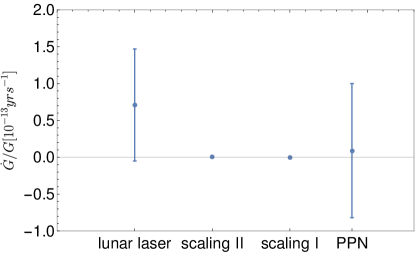
Figure 1: Values of the normalized derivative of the Newton constant G around z = 0, for both scaling relations labeled ”scaling-I” which is the proper distance scaling and ”scaling-II” the scaling using density. We include also the most recent observational values along with their error bars ($1\sigma$). These are: (a) from Fienga et al. (2014) via calculating possible impact of varying G on planetary orbits (labelled ’solar system orbits’) (b) from Hofmann and Müller (2018) using lunar laser ranging data (labelled ’lunar laser’).

Fig. (1) shows the comparison of these results with corresponding observations. As it is apparent from the latter figure, the evolution of G is within 1$\sigma$ of the observed values, for both scaling relations.

Scaling Model	$\xi\,\text{or}\,\tilde{\xi}$	$\tilde{\gamma}$	$\theta_{1}$	$\theta_{2}$
Cluster Radial Proper Distance ($\xi,\theta_{1},\theta_{2}$)	3.0	3.0	2.001	0.06
$>>$	1.0	0.1	2.005	0.05
Cluster Density Profile ($\tilde{\xi},\theta_{1},\theta_{2}$)	1e-28	10	2.001	0.06
$>>$	1e-28	15	2.005	0.05

Table 1: Indicative points on the parameter space for each of the two scaling relations (§42,63) that correspond to efficient phenomenology.

As another viability test for our models, we use the transition redshift, defined via the requirement $q(z_{tr})\equiv 0$. The latter corresponds to the moment of the transition between matter era and Dark Energy era in the cosmic history. In particular, using the plot of the deceleration parameter, q, (second column of Fig.(3) ) for these particular instances of the two different scaling expressions, we find the transition redshift. For the case of scaling with proper distance, we have $z_{tr}^{I}\simeq 0.8$ which lies within $\sim 3\sigma$ of both Jesus et al. (2020) results, obtained via a model independent method. For the case of scaling using density, we obtain $z_{tr}^{II}\simeq 1$ which again is statistically compatible with Jesus et al. (2020) results. From the latter fact we deduce that both models seem to be viable.

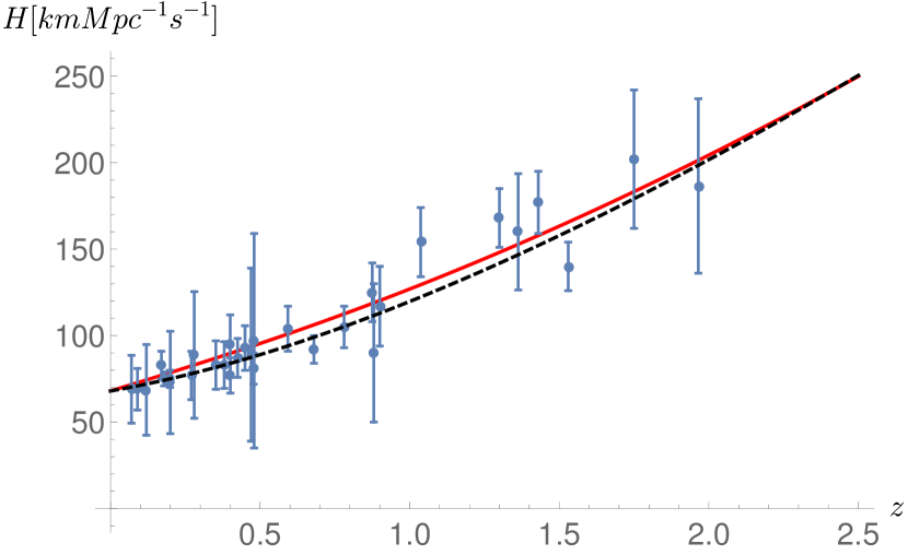
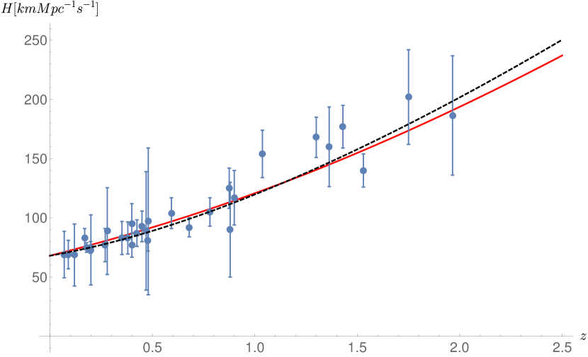
Figure 2: Plot of the Hubble rate along with a subset of the observational dataset, containing only data points obtained via the Cosmic Chronometers (CC) method, compiled at Yu et al. (2018). To allow direct comparison, we depict the Hubble rate of the concordance model (dashed black line) corresponding to the parameters set $\{\Omega_{m0},h\}=\{0.3,0.68\}$. The Hubble rate for each scaling relation is depicted with the solid line. In all cases the initial condition for the solution of proper distance was set to be $2r_{s}$, for reasons explained in the text. Left: Scaling using proper distance, for the parameter set $\{\Omega_{m0},\xi,h,\theta_{1},\theta_{2}\}=\{0.3,0.68,1,2.001,0.06\}$ Right: Scaling using density, for the parameter set $\{\Omega_{m0},h,\tilde{\xi},\theta_{1},\theta_{2}\}=\{0.3,0.68,10^{-28},2.005,0.05\}$

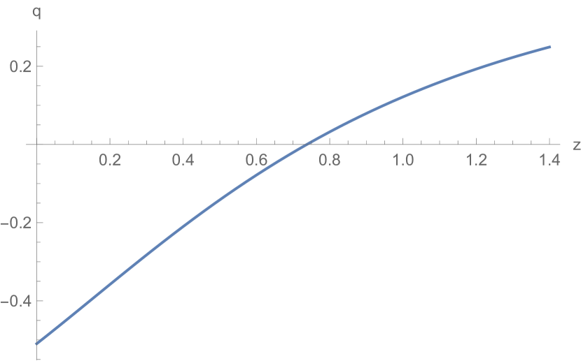
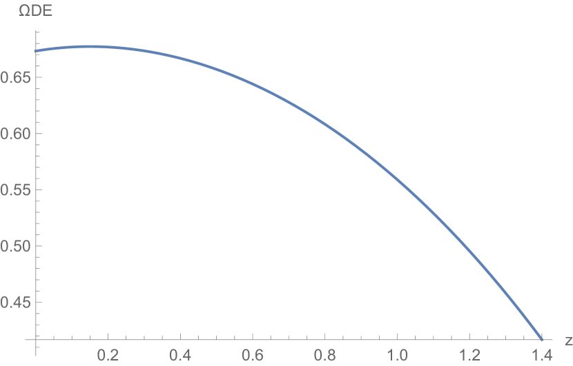
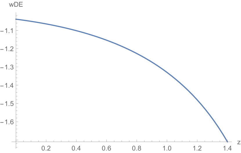
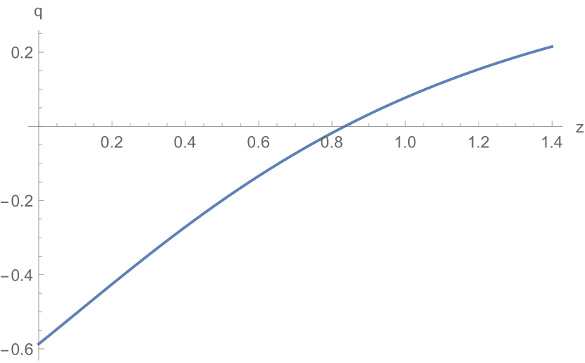
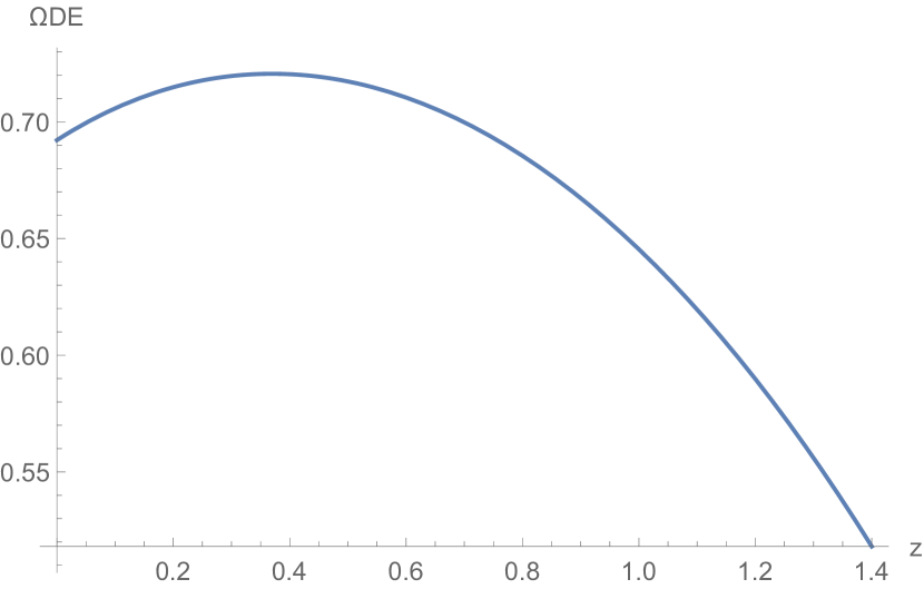
Figure 3: Plots of some representative cosmological parameters. From left to right: equation of state parameter for the effective Dark Energy fluid, $w_{DE}$, deceleration parameter, $q$ and normalized Dark Energy Density, $\Omega_{DE}$ as a function of the redshift $z$, for the two different scaling relations (top and bottom panel), see text. The parameters used for these plots are (top panel) $\Omega_{m0}=0.3,\ \xi=1,\ \theta_{1}=2.001,\ \theta_{2}=0.04$, (bottom panel) $\Omega_{m0}=0.3,\ \tilde{\xi}=10^{-28},\ \theta_{1}=2.005,\ \theta_{2}=0.06$.

V Conclusions

In this work we have extended the swiss-cheese models presented in Kofinas and Zarikas (2018); Anagnostopoulos et al. (2019b) to include an explicit running of $G$ according to the IR fixed point hypothesis. The presented analysis generalizes the original Einstein-Strauss model by considering an interior vacuole spacetime described by a RG-improved Schwarzschild spacetime in the presence of a cosmological constant and Newton’s constant that depend either on the proper distance $D_{s}$ , or on the matter density according to a RG trajectory for which both the dimensionless Newton constant and cosmological constant approach a fixed point at large distances.

The Darmois matching conditions determine the evolution of the FLRW spacetime outside the Schücking Radius. The RG trajectories emanating from the IR fixed point have been parametrized by two critical exponents $\theta_{1}$ and $\theta_{2}$ and by the scaling parameter $\xi$ which relates the RG cutoff $k$ with a characteristic distance scale. It turns out that the present phase of accelerated expansion is the result of the cumulative antigravity sources contribution within the Schücking radius. In particular no fine-tuning emerges at late times. Our formalism allows us also to take into account of the constraints on $\dot{G}/G$. Albeit the parameter space is large and a full numerical analysis is beyond the scope of the present work, it was possible to find many set parameters which reproduce the current $\Lambda CDM$ standard model. The results are very encouraging, as for both scaling expressions we do obtain reasonable behavior for the cosmological quantities $H(z),q,\,\,w_{DE},$ and $\Omega_{DE}$.

Interesting enough for the interesting cases both $\theta_{1}$ and $\theta_{2}$ can be taken as positive and this is consistent with the idea that the IR fixed point must be attractive in the $k\rightarrow 0$ limit. It would therefore be interesting to further test this cosmological model against the current observational data.

VI Acknowledgments

The authors acknowledge the support of the Faculty Development Competitive Research Grant Program (FDCRGP) Grant No. 110119FD4534. We are grateful to Alessia Platania for important remarks and comments on the manuscript.

References

- Rubin and Ford (1970) V. C. Rubin and J. Ford, W. Kent, LABEL:@jnlApJ 159, 379 (1970).
- Spergel et al. (2007) D. N. Spergel, R. Bean, O. Doré, M. R. Nolta, C. L. Bennett, J. Dunkley, G. Hinshaw, N. Jarosik, E. Komatsu, L. Page, et al., Astrophys. J., Suppl. Ser. 170, 377 (2007), eprint astro-ph/0603449.
- Straumann (1999) N. Straumann, Eur. J. Phys. 20, 419 (1999), eprint astro-ph/9908342.
- Wang et al. (2017) Q. Wang, Z. Zhu, and W. G. Unruh, Phys. Rev. D 95, 103504 (2017), eprint 1703.00543.
- Carlip (2019) S. Carlip, Phys. Rev. Lett. 123, 131302 (2019), eprint 1809.08277.
- Bonanno and Reuter (2002) A. Bonanno and M. Reuter, Phys. Lett. B 527, 9 (2002), eprint astro-ph/0106468.
- Bentivegna et al. (2004) E. Bentivegna, A. Bonanno, and M. Reuter, JCAP 01, 001 (2004), eprint astro-ph/0303150.
- Bonanno and Carloni (2012) A. Bonanno and S. Carloni, New Journal of Physics 14, 025008 (2012), eprint 1112.4613.
- Weinberg (1979) S. Weinberg, in General Relativity: An Einstein centenary survey, edited by S. W. Hawking and W. Israel (1979), pp. 790–831.
- Reuter (1998) M. Reuter, Phys. Rev. D 57, 971 (1998), eprint hep-th/9605030.
- Litim (2011) D. F. Litim, Phil. Trans. Roy. Soc. Lond. A 369, 2759 (2011), eprint 1102.4624.
- Nagy (2014) S. Nagy, Annals Phys. 350, 310 (2014), eprint 1211.4151.
- Bonanno and Saueressig (2017) A. Bonanno and F. Saueressig, Comptes Rendus Physique 18, 254 (2017), eprint 1702.04137.
- Percacci (2017) R. Percacci, An Introduction to Covariant Quantum Gravity and Asymptotic Safety, vol. 3 of 100 Years of General Relativity (World Scientific, 2017), ISBN 978-981-320-717-2, 978-981-320-719-6.
- Eichhorn (2019) A. Eichhorn, Front. Astron. Space Sci. 5, 47 (2019), eprint 1810.07615.
- Pereira (2019) A. D. Pereira, in Progress and Visions in Quantum Theory in View of Gravity: Bridging foundations of physics and mathematics (2019), eprint 1904.07042.
- Reuter and Saueressig (2019) M. Reuter and F. Saueressig, Quantum Gravity and the Functional Renormalization Group: The Road towards Asymptotic Safety (Cambridge University Press, 2019), ISBN 978-1-107-10732-8, 978-1-108-67074-6.
- Reichert (2020) M. Reichert, PoS 384, 005 (2020).
- Platania (2020) A. Platania, Front. in Phys. 8, 188 (2020), eprint 2003.13656.
- Polyakov (1993) A. M. Polyakov, in Les Houches Summer School on Gravitation and Quantizations, Session 57 (1993), pp. 0783–804, eprint hep-th/9304146.
- Codello and Percacci (2009) A. Codello and R. Percacci, Phys. Lett. B 672, 280 (2009), eprint 0810.0715.
- Reuter and Weyer (2004a) M. Reuter and H. Weyer, Phys. Rev. D 70, 124028 (2004a), eprint hep-th/0410117.
- Reuter and Weyer (2004b) M. Reuter and H. Weyer, J. Cosmol. Astropart. Phys. 2004, 001 (2004b), eprint hep-th/0410119.
- Reuter and Saueressig (2005) M. Reuter and F. Saueressig, JCAP 09, 012 (2005), eprint hep-th/0507167.
- Bonanno and Reuter (2007) A. Bonanno and M. Reuter, JCAP 08, 024 (2007), eprint 0706.0174.
- Kofinas and Zarikas (2016) G. Kofinas and V. Zarikas, Phys. Rev. D 94, 103514 (2016), eprint 1605.02241.
- Bonanno et al. (2018) A. Bonanno, G. Gionti, S. J., and A. Platania, Class. Quant. Grav. 35, 065004 (2018), eprint 1710.06317.
- Reuter and Weyer (2004) M. Reuter and H. Weyer, Phys. Rev. D 69, 104022 (2004), eprint hep-th/0311196.
- Bonanno et al. (2021) A. Bonanno, G. Kofinas, and V. Zarikas, Phys. Rev. D 103, 104025 (2021), eprint 2012.05338.
- Kofinas and Zarikas (2018) G. Kofinas and V. Zarikas, Phys. Rev. D 97, 123542 (2018), eprint 1706.08779.
- Mitra et al. (2021) A. Mitra, V. Zarikas, A. Bonanno, M. Good, and E. Güdekli, Universe 7, 263 (2021), eprint 2107.08519.
- Anagnostopoulos et al. (2019a) F. K. Anagnostopoulos, G. Kofinas, and V. Zarikas, Int. J. Mod. Phys. D 28, 14 (2019a), eprint 2102.07578.
- Anagnostopoulos et al. (2019b) F. K. Anagnostopoulos, S. Basilakos, G. Kofinas, and V. Zarikas, JCAP 02, 053 (2019b), eprint 1806.10580.
- Nagy et al. (2012) S. Nagy, J. Krizsan, and K. Sailer, JHEP 07, 102 (2012), eprint 1203.6564.
- Christiansen et al. (2014) N. Christiansen, D. F. Litim, J. M. Pawlowski, and A. Rodigast, Phys. Lett. B 728, 114 (2014), eprint 1209.4038.
- Biemans et al. (2017) J. Biemans, A. Platania, and F. Saueressig, Phys. Rev. D 95, 086013 (2017), eprint 1609.04813.
- Einstein and Straus (1946) A. Einstein and E. G. Straus, Annals of Mathematics pp. 731–741 (1946).
- Eisenhart (2016) L. P. Eisenhart, Riemannian geometry (Princeton university press, 2016).
- Balbinot et al. (1988) R. Balbinot, R. Bergamini, and A. Comastri, Phys. Rev. D 38, 2415 (1988).
- Darmois (1927) G. Darmois, Les équations de la gravitation einsteinienne (Gauthier-Villars Paris, 1927).
- Dyer and Oliwa (2000) C. C. Dyer and C. Oliwa (2000), eprint astro-ph/0004090.
- Koch and Saueressig (2014) B. Koch and F. Saueressig, Int. J. Mod. Phys. A 29, 1430011 (2014), eprint 1401.4452.
- Planck Collaboration et al. (2020) Planck Collaboration, N. Aghanim, Y. Akrami, M. Ashdown, J. Aumont, C. Baccigalupi, M. Ballardini, A. J. Banday, R. B. Barreiro, N. Bartolo, et al., Astron. Astrophys. 641, A6 (2020), eprint 1807.06209.
- Ringwald and Wetterich (1990) A. Ringwald and C. Wetterich, Nucl. Phys. B 334, 506 (1990).
- Alexandre et al. (1999) J. Alexandre, V. Branchina, and J. Polonyi, Phys. Lett. B 445, 351 (1999), eprint cond-mat/9803007.
- Bonanno and Lacagnina (2004) A. Bonanno and G. Lacagnina, Nucl. Phys. B 693, 36 (2004), eprint hep-th/0403176.
- Berges et al. (2002) J. Berges, N. Tetradis, and C. Wetterich, Phys. Rept. 363, 223 (2002), eprint hep-ph/0005122.
- Benedetti and Caravelli (2012) D. Benedetti and F. Caravelli, JHEP 06, 017 (2012), [Erratum: JHEP 10, 157 (2012)], eprint 1204.3541.
- Demmel et al. (2014) M. Demmel, F. Saueressig, and O. Zanusso, JHEP 06, 026 (2014), eprint 1401.5495.
- Dietz and Morris (2013) J. A. Dietz and T. R. Morris, JHEP 01, 108 (2013), eprint 1211.0955.
- Ohta and Yamada (2021) N. Ohta and M. Yamada (2021), eprint 2110.08594.
- Aliferis and Zarikas (2021) G. Aliferis and V. Zarikas, Phys. Rev. D 103, 023509 (2021), eprint 2006.13621.
- Zhao (1996) H. Zhao, Mon. Not. Roy. Astron. Soc. 278, 488 (1996), eprint astro-ph/9509122.
- Newman et al. (2013) A. B. Newman, T. Treu, R. S. Ellis, and D. J. Sand, Astrophys. J. 765, 25 (2013), eprint 1209.1392.
- Mitra and Linder (2021) A. Mitra and E. V. Linder, Phys. Rev. D 103, 023524 (2021), eprint 2011.08206.
- Linder and Mitra (2019) E. V. Linder and A. Mitra, Phys. Rev. D 100, 043542 (2019), eprint 1907.00985.
- Riess et al. (1998) A. G. Riess, A. V. Filippenko, P. Challis, A. Clocchiatti, A. Diercks, P. M. Garnavich, R. L. Gilliland, C. J. Hogan, S. Jha, R. P. Kirshner, et al., LABEL:@jnlAJ 116, 1009 (1998), eprint astro-ph/9805201.
- Perlmutter et al. (1999) S. Perlmutter et al. (Supernova Cosmology Project), Astrophys. J. 517, 565 (1999), eprint astro-ph/9812133.
- Alam et al. (2021) S. Alam et al. (eBOSS), Phys. Rev. D 103, 083533 (2021), eprint 2007.08991.
- Fienga et al. (2014) A. Fienga, J. Laskar, P. Exertier, H. Manche, and M. Gastineau (2014), eprint 1409.4932.
- Hofmann and Müller (2018) F. Hofmann and J. Müller, Class. Quant. Grav. 35, 035015 (2018).
- Bellinger and Christensen-Dalsgaard (2019) E. P. Bellinger and J. Christensen-Dalsgaard, Astrophys. J. Lett. 887, L1 (2019), eprint 1909.06378.
- Yu et al. (2018) H. Yu, B. Ratra, and F.-Y. Wang, Astrophys. J. 856, 3 (2018), eprint 1711.03437.
- Jesus et al. (2020) J. F. Jesus, R. Valentim, A. A. Escobal, and S. H. Pereira, JCAP 04, 053 (2020), eprint 1909.00090.