Tackling critical slowing down using global correction steps with equivariant flows: the case of the Schwinger model

Abstract

We propose a new method for simulating lattice gauge theories in the presence of fermions. The method combines flow-based generative models for local gauge field updates and hierarchical updates of the factorized fermion determinant. The flow-based generative models are restricted to proposing updates to gauge-fields within subdomains, thus keeping training times moderate while increasing the global volume. We apply our method performs to the 2-dimensional (2D) Schwinger model with $N_{f}=2$ Wilson Dirac fermions and show that no critical slowing down is observed in the sampling of topological sectors up to $\beta=8.45$. Furthermore, we show that fluctuations can be suppressed exponentially with the distance between active subdomains, allowing us to achieve acceptance rates of up to $99\%$ for the outer-most accept/reject step on lattices volumes of up to $V=128\times 128$.

Introduction. – Gauge field theories are solved non-perturbatively by defining them on a discrete spacetime lattice and carrying out a numerical evaluation, provided their infinite volume and zero lattice spacing limits are taken. These limits require simulation at fine lattice spacing, in order to access logarithmic corrections to discretization effects Husung et al. (2021). For example, in Quantum Chromodynamics (QCD), accessing quantities that can connect to experiments in the precision frontier requires sub-percent accuracy after combining statistical and systematic errors. Estimating reliably systematic errors includes extrapolation to the continuum limit. This systematic error is reduced by having lattice spacings smaller than 0.05 fm that is typically the smallest lattices spacing accessible to current simulations.

The Hybrid Monte Carlo (HMC) algorithm Duane et al. (1987); Gottlieb et al. (1987) has played an essential role in allowing for large scale simulations of lattice gauge theories. However, a major drawback is the so-called critical slowing down observed in simulations as the lattice spacing decreases. Critical slowing down is referred to as the exponential increase of the computational cost required for HMC to explore topological sectors of the theory as the lattice spacing is reduced Schaefer et al. (2011), thus resulting in a Markov Chain with long trajectories effectively that remain (frozen) in the same topological sector.

In Ref. Luscher (2010), it was shown how constructing a map that can trivialize a gauge-theory can be employed to solve topological freezing. A recent development Kanwar et al. (2020) was the application of a flow-based generative model built of machine trainable affine coupling layers that can be used to construct such a map showing how topological freezing is overcome as criticality is approached. A major obstacle in such machine learning approaches, however, is their scalability with the volume. Namely, while the number of degrees of freedom of the theory increases linearly with the volume, the trainable parameters and therefore the training time and memory requirements of the coupling layers scale polynomially. Indeed, as the volume is increased and more trainable parameters are introduced, convergence of the optimizer becomes non-trivial and requires extensive fine-tuning or pre-training techniques Del Debbio et al. (2021).

In this work, we introduce a novel approach that exploits locality so that the flow-based model proposes updates to subdomains of the lattice. Such approaches have traditionally been key drivers in the simulation of lattice gauge theories and lattice QCD in particular, allowing simulations at physical quark masses. Recent examples are multi-grid approaches Frommer et al. (2014); Lüscher (2004); Luscher (2007), efficient computation of the trace of the inverse Dirac operator using hierarchical probing Stathopoulos et al. (2013), and multi-level algorithms Cè et al. (2017, 2016), The new approach proposed here combines flow-based generative models for proposing gauge-filed configurations Kanwar et al. (2020) and hierarchical updating of the gauge-fields for including the fermion determinant Finkenrath et al. (2013). We illustrate that applicability of this method in the case of the 2D Schwinger model with two flavors of degenerate Wilson fermions ($N_{f}=2$). We show that this approach mitigates critical slowing down but also keeps high acceptance rates for volumes as large as 128$\times$128. In Fig. 1, we demonstrate that our method, denoted as “flowGC”, crucially increases the rate at which topological sectors of the theory are explored at very fine lattice spacings ($\beta=8.45$) where HMC is effectively frozen.

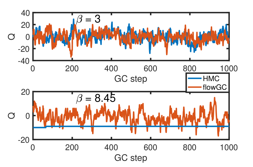
Figure 1: Monte Carlo history of the topological charge at a coarse lattice with $\beta=3$ (upper panel) and a fine lattice with $\beta=8.45$ (lower panel) at a volume of $V=128\times 128$ generated using the HMC algorithm and the flowGC method proposed.

Schwinger model – The Boltzmann factor of the discrete 2D Schwinger model can be written as

$$\rho(U)=\frac{1}{Z}\textrm{exp}\{-\beta S_{g}(U)+2\cdot\textrm{ln}\,\textrm{det}D(U)\}~{}.$$ (1)

For the ultra local pure gauge action, we employ the plaquette action $\beta S_{g}=\beta\sum_{i=1}^{V}\textrm{Re}[P(x)]$, where $V=L\cdot L$ is the lattice volume with lattice extent $L$ in each direction and $\beta$ is the gauge coupling. The plaquette at point $x$ is given by $P(x)=U^{\dagger}_{2}(x)U^{\dagger}_{1}(x+\hat{2})U_{2}(x+\hat{1})U^{\dagger}_{1}(x)$ with gauge links $U_{\nu}(x)\in U(1)$, which connects the point $x+\hat{\nu}$ with $x$. The plaquette is gauge invariant under an arbitrary gauge transformation $U_{\nu}(x)\rightarrow g(x+\hat{\nu})U_{\nu}(x)g(x)$ with $g(x)\in U(1)$. The topological charge takes integer values in the Schwinger model and can be defined by $Q=1/(2\pi)\sum_{i=1}^{V}(\arg(P(x))$, where $\arg(e^{i\theta})=\theta$. The fermion action is given by the determinant of the Wilson Dirac operator $D(U)\in\mathbb{C}^{2V\times 2V}$, which can be represented as a complex sparse matrix with a real determinant, see e.g. Ref. Christian et al. (2006).

Corrections via Metropolis accept/reject steps – Given a process $T_{0}(U\to U^{\prime})$, which allows proposing a new sample $U^{\prime}$ starting from a previous sample $U$ with known distribution $\tilde{\rho}(U^{\prime})$ and for which detailed balance is satisfied, a set of configurations $\{U\}$ weighted with a fixed point distribution $\rho(U)$ can be generated via a Markov chain. This is given by a combination of a proposal with a subsequent Metropolis accept/reject step

$$\begin{split}0)&\quad\text{Propose $U^{\prime}$ according to $T_{0}(U\to U^{\prime})$}\\ 1)&\quad P_{acc}(U\to U^{\prime})=\text{min}\left[1,{\frac{\tilde{\rho}(U)\rho(U^{\prime})}{\rho(U)\tilde{\rho}(U^{\prime})}}\,\right].\end{split}$$ (2)

Most Markov Chain Monte Carlo algorithms used for large scale simulations of lattice gauge theories, such as the HMC algorithm, are based on this approach, where the Metropolis accept/reject step works as a global correction (GC). In general, the Boltzmann factor $\rho$ depends on extensive quantities, i.e. the actions are extensive quantities, such as the corresponding variances scale with the physical volume. Assuming that the ratio of distributions $(\tilde{\rho}(U)\rho(U^{\prime}))/(\rho(U)\tilde{\rho}(U^{\prime}))$ is log-normal distributed, then for the acceptance rate $P_{acc}$ of Eq. (2), it follows that

$$P_{acc}=\textrm{erfc}\{\sqrt{\sigma^{2}(\Delta S)/8}\}$$ (3)

with the variance $\sigma^{2}(\Delta S)$, where $\Delta S=\textrm{ln}\{\rho(U^{\prime})\}-\textrm{ln}\{\rho(U)\}+\textrm{ln}\{\tilde{\rho}(U)\}-\textrm{ln}\{\tilde{\rho}(U^{\prime})\}$ Knechtli and Wolff (2003). The extensive character of $\Delta S$ implies that the acceptance rate drops exponentially as the volume increases. In order to achieve high acceptance rates, it is necessary to minimize the variance $\sigma^{2}(\Delta S)$, which can be done

• by using correlations between $\rho$ and $\tilde{\rho}$

• by reduction of the degrees of freedom of $\rho$ and $\tilde{\rho}$.

For HMC, case 1 above applies, namely the distance of $\rho$ and $\tilde{\rho}$ of the distribution of the Shadow Hamiltonian Clark and Kennedy (2007); Kennedy et al. (2013), is minimized. A combination of both cases leads to a generalization of the GC step of Eq. (2), which is achieved by introducing a hierarchy of filter steps. If we factorize the target fixed point distribution $\rho(U)$ into $n+1$ parts $P_{i}$ with

$$\rho_{j}(U)=P_{0}(U,\{\alpha^{(0)}\})\,P_{1}(U,\{\alpha^{(1)}\})\,\dots P_{j}(U,\{\alpha^{(j)}\})\,,$$ (4)

where $j\leq n$, $\rho_{n}(U)\equiv\rho(U)$ and $\{\alpha^{(j)}\}$ are arbitrary sets of parameters, then the GC step in Eq. (2) splits into $n$ successive steps, with the $j$^th given by

$$P^{j}_{acc}(U\to U^{\prime})= \text{min}\left[1,\frac{\rho_{j-1}(U)\rho_{j}(U^{\prime})}{\rho_{j}(U)\rho_{j-1}(U^{\prime})}\right]$$

$$= \text{min}\left[1,\frac{P_{j}(U^{\prime},\{\alpha^{(j)}\})}{P_{j}(U,\{\alpha^{(j)}\})}\right].$$ (5)

Now we can introduce a hierarchy of nested accept/reject steps which can be iterated to filter out local fluctuations effectively.

Flow-based generative models and trivializing maps – We employ gauge equivariant maps ($m(U)$) as in Ref. Kanwar et al. (2020), constructed by combining coupling layers $m=\prod_{j}g_{j}$. The map is required to transform gauge-fields from a trivialized phase of our gauge model with distribution $\rho_{trivial}$ into a non-trivial distribution $\tilde{\rho}$, i.e. $m(U):\,\rho_{trival}(U)\to\tilde{\rho}(U)$. Each coupling layer $g_{j}$ transforms a set of active gauge links using a set of gauge-invariant objects, such as plaquettes. The maps can be represented by tunable convolutional networks with few hidden layers Albergo et al. (2019); Dinh et al. (2017); Rezende and Mohamed (2016). Keeping track of the phase space deformation, this transformation can be computationally simplified using active, passive, and static masks, such that the Jacobian of the transformation becomes triangular. This yields a tractable determinant of the Jacobian of the transformation, which is needed to train the parameters of the coupling layers.

Now, we can write the distribution of the generative model as Albergo et al. (2019); Kanwar et al. (2020)

$$\tilde{\rho}(U)=\rho_{trival}(m^{-1}(U))\prod_{j}\textrm{det}J(g_{j}^{-1}(\{\alpha_{j}^{(0)}\}))$$ (6)

with the trivial distribution $\rho_{trivial}$ and the Jacobian $J(g_{j}^{-1}(\{\alpha_{j}^{(0)}\}))$ of each coupling layer. The parameters $\{\alpha_{j}^{(0)}\}$ are tunable weights in the coupling layers.

Minimizing directly the variance of the accept/reject step in (2) requires pairs of configuration $U,\,U^{\prime}$, with $U$ distributed via $\rho(U)$, which are apriory not available. It turns out that minimizing the difference between $\tilde{\rho}$ and ${\rho}$ is sufficient and leads to the definition of the loss-function as the Kullback-Leibler divergence

$$\textrm{loss}(U)=\textrm{ln}(\tilde{\rho}(U))-\textrm{ln}({\rho(U)}),$$ (7)

which can be now minimized by training through iteratively drawing random samples with $\rho_{trivial}$ and adjusting the weights $\alpha_{i,j}^{(0)}$ in the coupling layers.

Domain decomposition of gauge equivariant flows in the 2D Schwinger model. – In Refs. Kanwar et al. (2020); Albergo et al. (2021a), equivariant flows were introduced for generating field configurations of the 2D pure-gauge Schwinger model, demonstrating improved sampling of topological sectors at large values of the coupling, namely $\beta$=7, where HMC fails. Suppressing volume fluctuations within $\sigma^{2}(\textrm{loss})$, however, proved challenging for lattices with $L>16$, which is the interesting case. We will show that this can be addressed by splitting the accept/reject step in Eq. ((2)) using domain decomposition and, thus, limiting the dimension of $\tilde{\rho}$ to the size of the domains. Because the pure gauge action is ultra local, updates of links within domains can be carried out independently of other domains if links that lie in or at the boundary of the domains are kept constant. We employ equivariant flows that are trained to generate link variables within the domain, given a fixed set of links connecting the domains. To ensure ergoticity, we periodically shift the lattice by a random translations $T_{\vec{x}}:\vec{x_{0}}\to\vec{x_{0}}+\vec{x}$, similar to Ref. Luscher (2005). While the lattice action $\langle\rho(U)\rangle=\langle\rho(T_{\vec{x}}(U))\rangle$ is invariant under translation, the trained gauge equivariant map is apriori not $\langle\tilde{\rho}(U)\rangle\neq\langle\tilde{\rho}(T_{\vec{x}}(U))\rangle$. This means that after each shift, to calculate $\tilde{\rho}(U)$ we need to apply the reverse map $m^{-1}:U\to U_{trivial}$ to obtain the prior distribution. As an empirical check, we measure $\langle\tilde{\rho}(U)\rangle$ as we vary the frequency by which we shift the lattice, as shown in Fig. 2. We see that translations result in small fluctuations of the resulting distribution, indicating that no violation in translational invariance with statistical significance is observed.

To train the flow with fixed boundary conditions, we start from the software and workflow that implements the periodic boundary conditions followed in Ref. Albergo et al. (2021a). Namely, we train a flow using periodic boundary conditions for a lattice with dimensions $l\times l$, with $l$ being the lattice extent of the domains, i.e. the global lattice is constructed from $n\times n$ domains with $n=L/l$. The flow is then re-trained allowing only the links which do not enter the plaquettes and span boundaries to be updated. While training, the configurations in each batch use different boundary links but are kept constant between training iterations or epochs of one era. For each era, we re-generate boundary links using a flow trained with periodic boundary conditions. We use a batch size of 4096 and 1000 epochs per era. Indicatively, for $\beta=8.45$, training took about 14 hours on an NVIDIA V100 GPU, reaching an acceptance rate of 28% using $l=8$. With such a flow, trained for local updates and to which we can add random translations with minor effect on the resulting density, it is straightforward to generate ensembles of larger lattices, as demonstrated in Fig. 1 for $L$=128. Note that in order to change topological sectors, there is a lower bound on the physical domain size, which for this case ($l/\sqrt{\beta}=8/\sqrt{8.45}$) is satisfied.

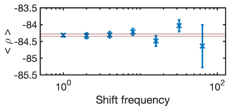
Figure 2: The flow distribution $\tilde{\rho}$ as a function of the number of iterations between random shifts of the lattice. For comparison the result for 1 shift per iteration is drawn with the horizontal band.

Global correction steps using fermions. – Integration of the fermions in the path integral yields the determinant of the Wilson Dirac operator as in Eq. 1, a non-local operator. Nonetheless, the fermion action can be splitted in a way that allows using Eq. (4) via a recursive Schur decomposition,

$$\textrm{det}D(U)=\textrm{det}\,\mathcal{S}(U)\cdot\prod_{i}\textrm{det}\,D(U^{(1)}_{i})$$ (8)

with the Schur complement that is defined on the even blocks, $\mathcal{S}(U)=1-D^{-1}(U^{(1)}_{e,e})D(U^{(1)}_{e,o})D^{-1}(U^{(1)}_{o,o})D(U^{(1)}_{o,e})$ and the block Dirac operators $D(U^{(1)}_{i})$ defined on a block. The superscript $(1)$ denotes the first level decomposition since the Schur decomposition can be applied recursively to multiple levels. Here we only use a single level. The decomposition effectively factorizes the long range modes, which are captured by the Schur complement, from the short range modes, captured by the block operators. Note that as in the gauge-field domain decomposition, the block operators only depend on links within a domain, that means they decouple exactly from each other. The procedure is perfectly suited to be used in a hierarchy of accept/reject filtering steps because it introduces additionally a computational cost ordering. The accept/reject steps of the block operators can be done in parallel and can be iterated to filter out larger local fluctuations of the determinant. In this work, the problem sizes are sufficiently small for LU-decomposition to be used for the determinant calculation. For systems with more degrees of freedom however, such as in lattice QCD, the determinant ratio can be estimated stochastic, as discussed in Ref. Finkenrath et al. (2013).

The Schur complement $\mathcal{S}(U)$ contains the interactions between the domains and, therefore, scales with the volume as an extensive quantity. The acceptance rate of the global correction step, thus, decreases exponentially with the volume. We mitigate this by introducing parameters to exploit correlations between the different factors of the action. Namely, a shift in the gauge coupling can be introduced between the pure-gauge action and the determinant

$$S(\beta,\Delta\beta)=(\beta+\Delta\beta)S_{g}+S_{f}$$ (9)

with $S_{f}=-2\cdot\textrm{ln}\,\textrm{det}D(U)$. The variance of the action is minimized when $\Delta\beta$ fulfills the relation

$$\Delta\beta=-\textrm{cov}(S_{g},S_{f})/\sigma^{2}(S_{f}),$$ (10)

with $\textrm{cov}(x,y)$ the covariance of $x$ and $y$. One way to use this feature is, for example, to generate flow based updates of the domains using $\beta+\Delta\beta$ as the coupling and reweighting back to the target coupling $\beta$ during the accept/reject step of the global correction. In our algorithm, which as will be explained includes four accept/reject steps, we generalize this approach by allowing for a different $\Delta\beta$ at each step Finkenrath et al. (2013). Details of the steps and the values of $\Delta\beta$ used are given in the Supplemental Material.

To further improve the global acceptance rate we note that domains decouple effectively exponentially with their distance via $\propto\textrm{exp}(-c_{0}\;m_{PS}\cdot|x-y|)$ and the effective decoupling length, therefore, depends on the lowest physical mode, i.e. the pseudoscalar mass $m_{PS}$ Luscher (2003); Cè et al. (2017). We, thus, increase the distance between domains being updated by generalizing the checkerboard coloring of the blocks to four colors and only update domains of same color, while all others are kept constant. In two dimensions this is possible if the decomposition is such that it yields an even number of domains in each direction. The global acceptance rate can now be further increased by introducing an additional intermediate step, which includes corrections from the eight blocks surrounding the block being updated, i.e. a $3L_{b}\times 3L_{b}$ operator, with the active $L_{b}\times L_{b}$ block located in the center. We model the variance of the global GC step as

$$\sigma^{2}(V,\beta,d,m_{PS})=\frac{A\cdot V}{m_{PS}\beta^{3/2}}\cdot\textrm{exp}\{-B\cdot d\;m_{PS}\},$$ (11)

where $d$ is the distance between active domains and find $A=0.0030(1)$ and $B=2.4062(59)$. From now on, the method described will be referred to as a 5-level flowGC algorithm, which includes the following steps:

• Flow proposal to generate 100 samples within each active block with $l=8$

• Accept/reject step over the 100 samples using the pure gauge action of the active blocks as target probability and keeping the final accepted configuration. The acceptance rate is $P^{(1)}_{acc}\sim 0.25$.

• Calculation of the determinant of the block operator $D(U_{j})$ with $L_{b}=n\cdot l$ with $n\in 1,2,\ldots$ and accept/reject. Repeat, starting from step 0. and repeat two to four times. The acceptance rate with $n=2$ is $P_{acc}^{(2)}\sim 0.7$.

• Calculation of the extended $3L_{b}\times 3L_{b}$ Dirac operator and performance of an accept/reject step. Repeat, starting from step 0. twice. The acceptance rate is $P_{acc}^{(3)}\sim 0.75$.

• Calculation of Schur complement term performing a global accept/reject step correcting to the target probability $\propto\textrm{exp}\{-\beta S_{g}+S_{f}\}$.

The significance of including steps 2. and 3. should be stressed here, since not including them results in an acceptance rate that quickly decreases with increasing volume, as shown in Fig. 3. Note that for the 5-level flowGC algorithm studied here, 15.6% of the gauge links are updated in each global iteration step. When varying the block sizes of the fermion determinant domains, $L_{b}$, the total ratio does not change since we keep the flow based proposal fixed to $l=8$ blocks for the flow update in step 1. Therefore, the improvement of the acceptance rate observed as we increase the domain block sizes ($L_{b}=8$, $L_{b}=16$, and $L_{b}=32$ in Fig. 3) is due to the increased distance between active domains and the effectiveness of the filtering applied in step 3. From this analysis, we conclude that for a lattice of size $L=128$ we can achieve $P_{acc}>0.97$ for distances $d\gtrsim 16$.

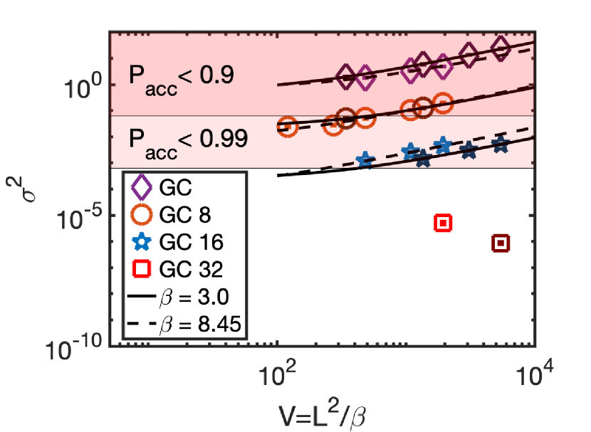
Figure 3: The variance of the global correction step as a function of the global volume ($V/\beta$) for $\beta=3$ (darker points) and $\beta=8.45$ (lighter points). We show the naive global correction step GC without hierarchical filtering of the block and extended block operator (diamonds), as well as for the 5-level flowGC algorithm with block distance $L_{b}=8$ (circles), with $L_{b}=16$ (stars), and with $L_{b}=32$ (square).

Table 1: The coupling $\beta$ and bare fermion mass $m_{0}$ used for three representative $N_{f}=2$ ensembles of the total generated. We also show the measured plaquette ($P$) and topological charge ($Q^{2}$). For the ensembles with gauge couplings $\beta\in[1,\,6]$ we set the parameters as in Ref. Christian et al. (2006), while for the finer lattice $\beta=8.45$ we refer to Ref. Albandea et al. (2021).

$\beta$	$m_{0}$	$am_{PS}$	$P$	$Q^{2}$
3.0	-0.082626	0.2241(38)	0.82705(12)	67.6(112)
6.0	-0.034249	0.1649(23)	0.91659(10)	24.3(  24)
8.45	0.0	0.1951(17)	0.94084(  7)	21.9(  25)

Markov Chain Monte Carlo simulations with dynamical fermions. – We generate Markov chains with $\beta\in[1.0,\,8.45]$ and lattice sizes of $L/\beta\in[22,\,74]$. The gauge coupling range spans from values where topological sampling is possible using HMC ($\beta\in[1,\,4]$) to values where with HMC we observe the onset of critical slowing down ($\beta\in[4,\,6]$) as well as values of $\beta>6.00$, where the HMC algorithm effectively freezes. In Table 1, we list the parameters and observables measured for three values of $\beta$ that are representative of these three regions. To compare how well the topological charge is sampled, we measured the so-called tunneling rate per global acceptance step via

$$T(Q)=\langle|Q_{i}-Q_{i+1}|\rangle.$$ (12)

We choose this quantity rather than the auto-correlation time to compare the topological sampling behavior of the different algorithms, since it increases with the lattice extent $L/\sqrt{\beta}$. It is also easier to estimate for cases with few changes in the topological charge, namely for HMC when $\beta=8.45$. For the HMC, $Q_{i}$ are separated by one molecular dynamics update with the acceptance rate tuned to $P_{acc}>90\%$, while for the 5-level flowGC we separate with one global correction step and use a gauge flow with $l=8$ domains, meaning at most 15.6% of the links are updated per step. As shown in Fig. 4, the tunneling rate for the 5-level flowGC algorithm remains constant over the $\beta$ values simulated, and is consistent with the rate achieved by HMC at $\beta=3.0$. HMC appears to be more favorable for the cases $\beta<2$, however only by a factor of at most two, while the 5-level flowGC achieves over two orders of magnitude better tunneling rate for $\beta>6$.

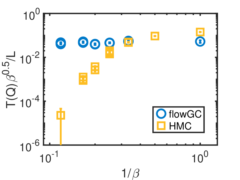
Figure 4: Tunneling rate of the topological charge per update versus the inverse coupling for the 5-level flowGC algorithm (circles) with $l=8$ flow proposals and $L_{b}=16$ and the HMC algorithm (squares). We normalize the tunneling rate with the volume and scale with $\sqrt{\beta}$ to derive a dimensionless quantity.

Conclusion. – We present a novel algorithm for effectively simulating lattice gauge theories with fermions. The algorithm comprises of gauge equivariant flows for updating sub-domains of the global lattice combined with hierarchical blocking of the fermion determinant followed by a global correction step. We derive a 5-level flowGC algorithm, which is shown to overcome critical slowing down in the Schwinger model with two degenerate flavors of fermions. In addition, domain decomposition allows scaling to large lattice sizes illustrating the effectiveness of the algorithm by simulating up to $128\times 128$ lattices. The variance of the global correction step is found to decrease exponentially with the distance $d$ between active blocks, i.e. $\sigma^{2}\propto V/(m_{PS}\beta^{3/2})\cdot\textrm{exp}(-2d\cdot m_{PS})$, with $m_{PS}$ the pseudoscalar mass. Such a dependence with $d$ enables us to tune the block sizes $L_{b}$ for a given minimum distance $d$. We demonstrate the approach by comparing the tunneling rate of the topological charge achieved by our method and HMC and show that the 5-level flowGC algorithms achieves orders of magnitude higher tunneling rate at $\beta=8.45$ where HMC freezes.

The 5-level flowCG algorithm can be extended to 4D and gauge theories of larger gauge groups, such as lattice QCD. However, a number of additional challenges may need to be addressed, such as a possible deterioration of the acceptance rate due to the larger block sizes Finkenrath et al. (2013) that may be needed for decoupling domains in simulations with physical quark masses. Including the block determinant into the training, as in Ref. Albergo et al. (2021b) could address this issue. Furthermore, the algorithm can be made more efficient when combined with HMC, similar what is discussed in Ref. Albandea et al. (2021). It may be possible, if topological freezing is resolved, to restore the sampling rate as expected from the Langevin class of algorithms, which might increases with the inverse lattice spacing squared $a^{-2}$ Baulieu and Zwanziger (2000); Luscher and Schaefer (2011).

Supplemental Material: Details on runs with global fermionic correction steps

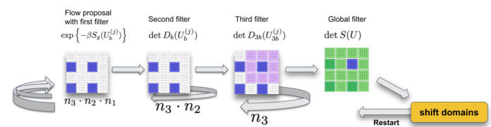
Figure 5: The schema illustrates the different levels of the 5 level flowGC algorithm.

Details on runs with 5 level flowGC algorithm. – For the global correction step algorithm driven by the gauge equivariant flow the target Boltzmann weight is given by

$$P(U)=Z^{-1}\left(\prod_{j}^{N_{f}}\textrm{det}D_{j}(U)\right)e^{-\beta S_{g}(U)}$$ (13)

with the partition sum $Z$, which we will drop from now on. Now, using domain decomposition we can split the action into

$$\begin{split}\rho(U)=&\quad P^{(4)}\cdot\prod_{j=1}^{N_{b}}\left(P^{(3)}_{j}P^{(2)}_{j}\prod_{k=1}^{N_{l}}P^{(1)}_{k,j}\right)\\ =&\quad\textrm{det}\,D^{2}(U)\cdot\textrm{exp}\{-\beta S_{g}(U)\}\end{split}$$ (14)

where the parts $P^{(3)}_{j},P^{(2)}_{j},P^{(1)}_{k,j}$ does not include links of other active domains $i$ with $i\neq j$.

Now, we can introduce a 5 level hierarchical filter step with the distributions

$$\begin{split}0)&\quad\tilde{\rho}=\rho_{trival}(m^{-1}(U_{l}^{(k,j)}))\prod_{i=0}^{N_{coupling}}\textrm{det}J(g_{i}^{-1}(\{\alpha_{i}^{(0)}\}))\\ 1)&\quad P^{(1)}_{k,j}=\textrm{exp}\left\{-\left(\beta-\sum_{i=2}^{N_{lvl}}\delta\beta_{i}^{(1)}\right)S_{g}(U_{l}^{(k,j)})\right\}\\ 2)&\quad P^{(2)}_{j}=\textrm{exp}\left\{2\left(1-\sum_{i=3}^{N_{lvl}}\delta\beta_{i}^{(2)}\right)\cdot\textrm{ln}\,\textrm{det}\,D_{b}(U_{L_{b}}^{(j)})-\delta\beta_{2}^{(1)}\sum_{k=1}^{N_{l}}S_{g}(U_{l}^{(k,j)})\right\}\\ 3)&\quad P^{(3)}_{j}=\textrm{exp}\left\{-\delta\beta_{4}^{(3)}\cdot\textrm{ln}\,\textrm{det}\,D_{3b}(U_{3L_{b}}^{(j)})+\delta\beta_{3}^{(2)}\cdot\textrm{ln}\,\textrm{det}\,D_{b}(U_{L_{b}}^{(j)})-\delta\beta_{3}^{(1)}\sum_{k=1}^{N_{l}}S_{g}(U_{L_{b}}^{(k,j)})\right\}\\ 4)&\quad P^{(4)}=\textrm{exp}\left\{2\cdot\textrm{ln}\,\textrm{det}\,S(U)+\sum_{j=1}^{N_{b}}\left[\delta\beta_{4}^{(3)}\textrm{ln}\,\textrm{det}\,D_{3b}(U_{3L_{b}}^{(j)})+\delta\beta_{4}^{(2)}\textrm{ln}\,\textrm{det}\,D_{b}(U_{L_{b}}^{(j)})-\delta\beta_{4}^{(1)}\sum_{k=1}^{N_{l}}S_{g}(U_{L_{b}}^{(k,j)})\right]\right\}\end{split}$$ (15)

with $N_{lvl}$ the number of levels, $N_{l}$ the number of subdomains within a block of length $L_{b}$ and $N_{b}$ the number of active blocks. Step 0) to 3) can be performed for each block $j$ or $k$ independently while only step 4) includes global correlations. Note that if $L_{b}>8$ the domain $L_{b}\times L_{b}$ is further decomposed into $l\times l$ subdomains with $l=8$. Step 0) and 1) is then performed on each subdomain $k$ individual. Each step can be iterated as illustrated in Fig. 5.

Parameter tuning. – Now, the parameters $\delta\beta_{i}^{(j)}$ can be tuned by minimizing the variance of the higher level accept/reject steps utilizing the co-variance between the different action parts, see also Ref. Finkenrath et al. (2013). We can write the action of the $i$th level step as

$$S_{i}(U)=\sum_{j=0}^{i}\beta_{i}^{(j)}S^{(j)}(U),\qquad\quad i=1,2,\ldots,n$$ (16)

with the difference of the actions

$$\Delta_{i}=S_{i}(U^{\prime})-S_{i}(U).$$ (17)

Now, we can introduce a cost-ordered hierarchy, where the more expensive, larger term, such as the Schur complements do not enter the low level accept–reject steps. This implies $\beta_{i}^{(j)}=0$ for $i<j$. Moreover, the additional parameters have to sum up to the target parameters, namely $\sum_{i=1}^{n}\beta_{i}^{(j)}=\beta^{(j)}$.

Now, minimizing the variance starting from the top level leads to a coupled linear systems which can be exactly solved. The system of linear equations is given in the order $i=n,n-1,\ldots,1$ by

$$2C^{(jj)}\beta_{i}^{(j)}+\sum_{\underset{k\neq j}{k=0}}^{i}C^{(jk)}\beta_{i}^{(k)}=-C^{(ji)}\beta_{i}^{(i)},\quad j=0,\cdots,i-1$$ (18)

with the co-variance $C^{jk}=\langle\Delta^{(j)}\Delta^{(k)}\rangle-\langle\Delta^{(j)}\rangle\langle\Delta^{(k)}\rangle$ of the difference $\Delta^{(j)}=S^{(j)}(U^{\prime})-S^{(j)}(U)$. Implying the constrain $\beta_{i}^{(i)}=\beta^{(i)}-\sum_{j=i+1}^{n}\beta_{j}^{(i)}$ the linear equation system eq. (18) can be solved, resulting into $\beta_{i}^{(0)},\ldots,\beta_{i}^{i-1}$. We present in table 2 the optimal parameters for the runs with $d=16$ and $L=128$ at the three different gauge couplings $\beta=3.0,6.0,8.45$ with Wilson mass parameters $m_{0}=-0.082626,-0.034249,0.0$, respectively. The parameters nicely illustrate the correlations between the different parts of the fermion action, i.e. roughly the full contribution of $\textrm{log}\,P^{(2)}_{j}$ is compensated within $\textrm{log}\,P^{(3)}_{j}$ and similar for $\sum_{j}\textrm{log}\,P^{(3)}_{j}$ within $\textrm{log}\,P^{(4)}$. In general, by including fermions the gauge coupling of the pure gauge proposal shifts towards larger values. That is expected, i.e. first contribution of the so-called hopping parameter expansion of the determinant of $D$ comes with a positive contribution of $S_{g}$.

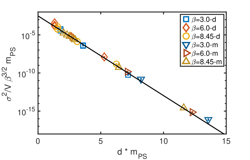
Figure 6: The fit shows the dependence of the variance of the global correction steps, within the 5 level flowGC algorithm on the distance between active blocks $d/\sqrt{\beta}$, on the pseudoscalar meson mass $m_{PS}\sqrt{\beta}$ and the volume $V/\beta$. The runs with different distances, denoted as -d are performed at parameters listed in Tab. 1 while runs with different pseudoscalar masses are denoted by -m and performed at constant $d=16$ and lattice extend $L=64$ at the three different $\beta$ values.

Dependencies of the variance. – To estimate dependencies of the variance in the final global correction step of the 5 level flowGC we generated a set of 35 simulations at different gauge couplings $\beta=3.0,6.0,8.45$, different volumes with $L=64,96,128$, different distances $d=8,16,32$ and various pseudoscalar masses between $am_{PS}\in[0.12,\;0.73]$ using $l=8$ gauge flow updates. We found

$$\sigma^{2}=A\cdot\frac{V}{m_{PS}\beta^{3/2}}\;\cdot\textrm{exp}\{-B\cdot d\,m_{PS}\}$$ (19)

with $A=0.0030(1)$ and $B=2.4062(59)$. The dependence is depict in Fig. 6 for the distance $d$ and the pseudoscalar mass $m_{PS}$, while the dependence on the volume $V$ and gauge coupling $\beta$ is shown in Fig. 3. The fit in $d\cdot m_{PS}$ with $\chi^{2}/dof=21$ captures the overall dependence quite well. Note that, although we employ flow updates of domain with $l=8$, for smaller pseudoscalar masses as well as for smaller $\beta$ the acceptance rate of the lower filter might drop such that the overall updated fraction of the gauge links can drop under 15.6%. This leads to a smaller variance $\sigma^{2}$, which is the case for most of the $\beta=3.0$ runs. This makes it difficult to estimate the direct pseudoscalar mass dependence, i.e. if we optimize the leading $am_{PS}$ dependence of $\sigma^{2}$ via the minimal $\chi^{2}$, we find $\sigma^{2}\propto 1/(m_{PS}\sqrt{\beta})^{x}$ with $x=1.2$.

Note that the exponential suppression with the distance of the global filter step, lead to an exponential increase of the fourth filter step. However, because the corresponding term only contains contribution from a single active domain, this can be mitigated via additional iterations on the last filter level.

$\beta$	3.0	6.0	8.45
5 level flowGC with $d=16$:
Level 4
with $\sigma^{2}$	0.0052	0.0369	0.0046
and $P_{acc}$	0.9713	0.9235	0.9727
$\delta\beta_{4}^{(3)}$	-2.0037	-2.0182	-2.0087
$\delta\beta_{4}^{(2)}$	1.0027	1.0061	1.0083
$\delta\beta_{4}^{(1)}$	-0.0003	0.0008	0.0004
Level 3	$n_{1}=2$
with $\sigma^{2}$	0.6688	0.6190	0.1546
and $P_{acc}$	0.6826	0.6940	0.8441
$\delta\beta_{3}^{(2)}$	-1.1730	-1.3635	-1.3534
$\delta\beta_{3}^{(1)}$	-0.0006	0.0149	0.0125
Level 2	$n_{2}=4$
with $\sigma^{2}$	1.4384	0.8325	0.1857
and $P_{acc}$	0.5487	0.6482	0.8294
$\delta\beta_{2}^{(1)}$	-0.2482	-0.3082	-0.2863
Level 1	$n_{1}=100$
with $P_{acc}$	0.5669	0.2501	0.2794
2 level GC:
with $\sigma^{2}$	12.3774	9.7119	3.7260
and $P_{acc}$	0.0786	0.1192	0.3345

Table 2: The table shows the parameter which minimize the variance of each filter step. The parameter used for the runs with coupling constant $\beta=3.0,\,6.0,\,8.45$ using a lattice extend of $L=128$ with a distance $d=16$ between active domains, by keeping the domain size at a similar size $L_{b}=16$. For comparison numbers of a two level global correction step are included, which is driven by an HMC update and a global correction step without hierarchical filter steps.

Remarks on cost scaling. – The computational cost of the flowGC algorithm during the Monte Carlo sampling depends mainly on the acceptance rate and the calculation of the determinant ratios. Towards larger lattices, higher dimensions and gauge theories of larger gauge groups, such as lattice QCD, the calculation of the determinants ratios requires alternative methods. A possible way out is based on stochastic estimation which can be used within the hierarchical filter steps, as discussed in Ref. Finkenrath et al. (2013). The stochastic noise scales, similar to the exact weight, with the volume.

Thus the computational cost for a gauge theory in $D$ dimensions is given by

$$\begin{split}\textrm{cost}\propto&\left(c_{3d}\frac{N_{b}\cdot n_{3}\cdot V_{3d}}{a^{D}}+c_{gl}\frac{V_{gl}}{a^{D}}\right)\,\cdot\\ &\quad 1/\textrm{erfc}\left\{\left[\frac{A^{\prime}\cdot V}{8m_{PS}a^{D+1}}e^{-B^{\prime}\cdot d\,m_{PS}}\right]^{1/2}\right\}\end{split}$$ (20)

with $N_{b}$ the number of active domains, $n_{3}$ the number of update iteration of filter step at level 3, with $V_{3d}/a^{D}$ the volume of the extended block operator, which filter out the long range fluctuations of the active blocks and $V_{gl}/a^{D}$ the global volume. The coefficients $A^{\prime}$ and $B^{\prime}$ are model dependent and the factors $c_{3d}$ and $c_{gl}$ are relative cost factors, e.g. includes the total number of inversions needed for the stochastic determinant estimation. For high acceptance the computational cost is likely to be dominated by the extended block operator with $V_{3d}/a^{D}$ if large distances $d$ are neccessary to compensate small pseudoscalar masses. Note that it is possible to introduce additional filter levels via recursive Schur decomposition, if the corresponding acceptance rate drops.

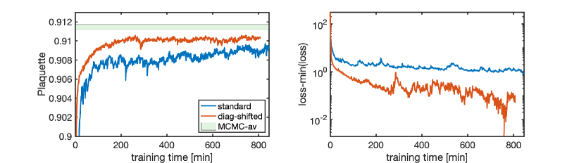
Figure 7: The figure shows the comparison of the training effectiveness using the standard masks compared to the optimised version, with diagonal shifted masks. Left panel shows the plaquette average of each batch after one epoch, while the right panel depict the minimization of the loss function in dependence of the training time in case of periodic boundary condition.

Remarks on masks in gauge invariant flows. – The flow maps are constructed of coupling layers, which maps the links towards the target distribution. For simplified computation of the Jacobian, only a couple of links are updated in each transformation. Here, we use plaquettes as the gauge invariant objects Kanwar et al. (2020); Albergo et al. (2021a); Boyda et al. (2021). Using gauge invariant objects results then into three different subsets or masks within the coupling layers, namely

• frozen, which are used for updating

• active, which are getting updated

• passive, which are updated passively.

Within the original proposal Albergo et al. (2021a), the lattice were divided vertical into columns, starting with a passive column, followed by an active and two frozen columns, as illustrated within the left panel of Fig. 8. Now, the links laying between the passive and active columns can be updated based on the trainable coupling layers with input from the frozen links.

After an update step, the maps are rotated and the links in opposite direction are updated. This is iterated until all links are updated, which need an application of 8 coupling layers in two dimensions.

We increased convergence by shifting the masks diagonal, as illustrated on right panel in Fig. 8. This increases overlap with frozen plaquettes in case of a kernel size of 3 for the employed convolutional networks within the coupling layers and results into faster convergence at similar training time, as shown in Fig. 7. For the training, we increased the number of layers to 64 while keeping other parameter, such as the hidden layers $(8,8)$ or the convolutional kernels size $3$ similar to the original default values, see Ref. Albergo et al. (2021a).

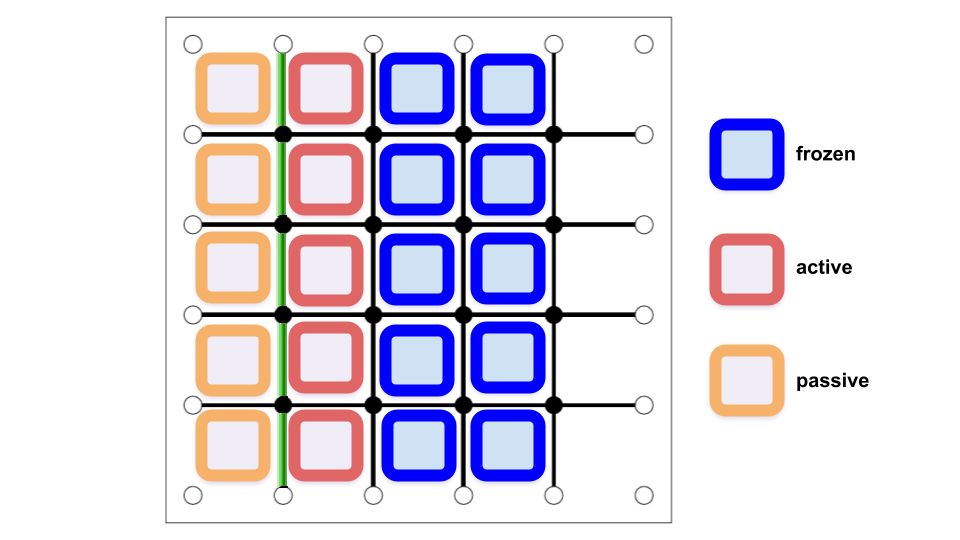
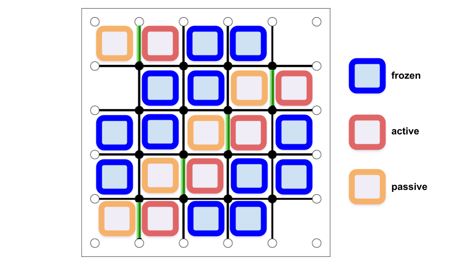
Figure 8: The figure shows the mask setup used in the gauge equivariant flows. The original approachAlbergo et al. (2021a) is shown in the left panel, while faster convergence can be achieved with the diagonal shifted approach (right panel).