Eclipse Mapping of EXO 0748$-$676: Evidence for a Massive Neutron Star

Abstract

Determining the maximum possible neutron star (NS) mass places limits on the equation of state (EoS) of ultra-dense matter. The mass of NSs in low mass X-ray binaries can be determined from the binary mass function, providing independent constraints are placed on both the binary inclination and mass ratio. In eclipsing systems, they relate via the totality duration. EXO 0748$-$676 is an eclipsing NS low mass X-ray binary with a binary mass function estimated using stellar emission lines from the irradiated face of the companion. The NS mass is thus known as a function of mass ratio. Here we model the X-ray eclipses in several energy bands, utilising archival XMM-Newton data. We find a narrow region of absorbing material surrounding the companion star is required to explain the energy-dependent eclipses. Therefore, we suggest the companion may be experiencing ablation of its outer layers and that the system could transition into a redback millisecond pulsar. Our fit returns a mass ratio of $q=0.222^{+0.07}_{-0.08}$ and an inclination $i=76.5\pm^{1.4}_{1.1}$. Combining these with the previously measured radial velocity of $410\pm 5$ km/s, derived from Doppler mapping analysis of H_α emission during quiescence, returns a NS mass of $\sim 2~{}M_{\odot}$ even if the line originates as far from the NS as physically possible, favouring hard EoS. The inferred mass increases for a more realistic emission point. However, a $\sim 1.4~{}M_{\odot}$ canonical NS mass is possible when considering radial velocity values derived from other emission lines observed both during outburst and quiescence.

1 Introduction

Observing neutron star (NS) low-mass X-ray binaries (LMXBs) provides an opportunity to constrain the equation of state (EoS) of matter at extreme densities and develop binary evolution models (Steiner et al., 2010; Providência, 2019; Podsiadlowski, 2009; Postnov & Yungelson, 2014). Since the EoS (the pressure-density relation) uniquely predicts the NS mass-radius relation (Lindblom 1992; see Fig 10 of Voisin et al. 2020 for some up-to-date examples), it can be constrained from measurements of the mass and radius of astrophysical NSs. Mass alone can be highly constraining since each EoS predicts a maximum possible NS mass. Observationally determining the maximum NS mass also informs stellar evolution models (Antoniadis et al., 2016; Sukhbold et al., 2018; Raithel et al., 2018) and the interpretation of gravitational wave observations (Yang et al., 2018; Essick & Landry, 2020; Chen & Chatziioannou, 2020), both of which typically assume that compact objects with mass $<3~{}M_{\odot}$ are NSs, with the remainder being black holes (BHs). For example, GW190425 (Abbott et al., 2020a) was classified as the coalescence of two NSs because the mass of the primary was $\sim 2.5M_{\odot}$, but no electromagnetic signatures were detected to confirm a NS was present. To date, the most massive confirmed NS is PSR J0740+6620 at $M_{\rm ns}\sim 2.1M_{\odot}$ (Cromartie et al., 2019; Fonseca et al., 2021; Coleman Miller et al., 2021). The recent detection of GW190814 (Abbott et al., 2020b), classified as the merger of a $\sim 2.6M_{\odot}$ NS and $\sim 5M_{\odot}$ BH contests this, suggesting that NSs can exist within the so-called mass-gap and impacting the inferred nucleonic EoS (Fattoyev et al., 2020).

There are many methods used to estimate the mass and/or radius of a NS (see Coleman Miller 2013 or Özel & Freire 2016 for a summary). Waveform modelling of X-ray pulsations (or thermonuclear burst oscillations), from either isolated or accreting NSs, provides constraints on both mass and radius because the waveform is distorted by Doppler shifts from NS rotation and gravitational redshift (Van Paradijs, 1979; Fujimoto & Taam, 1986; Sztajno et al., 1987; Poutanen & Gierliński, 2003; Riley et al., 2019). Alternatively, the NS radius can be estimated by combining the temperature and observed flux of thermal emission from the NS’s surface with a distance estimate. Photospheric radius expansion (PRE) bursts from LMXBs enable a mass estimate by assuming that the burst occurs when the NS is accreting at the Eddington luminosity (Damen et al., 1990; Lewin et al., 1993; Özel, 2006; Güver et al., 2010). The mass of NSs in binary systems can be constrained dynamically by measuring Doppler shifts caused by the orbital motion of one of the binary components. This is the most direct method of measuring NS mass as it assumes only Kepler’s laws. For pulsating NSs the Doppler shifts can be measured from orbital phase-dependent shifts to the pulse frequency (Chakrabarty & Morgan, 1998), and for quiescent systems, they can be measured from orbital phase-dependent shifts to the wavelength of lines in the spectrum of the companion star (the radial velocity curve; e.g. Casares et al. 2014). In both cases the actual observable is the binary mass function, which depends on NS mass, $M_{\rm ns}$, mass ratio, $q=M_{\rm cs}/M_{\rm ns}$ where $M_{\rm cs}$ is the companion star mass, and binary inclination angle, $i$. In the latter case, the binary mass function is given by

$$f=\frac{PK^{3}}{2\pi G}=\frac{M_{\rm ns}\sin^{3}i}{(1+q)^{2}},$$ (1)

where $P$ is the orbital period, $G$ is Newton’s gravitational constant and $K$ is the semi-amplitude of the radial velocity curve. The degeneracy between mass, mass ratio and inclination is partially broken in eclipsing systems, in which $q$ and $i$ are related via the duration of totality, $t_{e}$, if the companion star is filling its Roche-Lobe (Horne, 1985). The NS’s mass in an eclipsing system with a measured binary mass function is therefore known as a function of $q$.

Here we consider the LMXB EXO 0748$-$676, which underwent a $>20$ yr outburst (Parmar et al., 1986) during which many eclipses with $t_{e}\approx 500$ s were observed by EXOSAT, RXTE and XMM-Newton, recurring on the orbital period of $P=3.824$ hrs (Parmar et al., 1986; Wolff et al., 2009). Pulsations have never been detected from the source, but the NS spin frequency is likely within a few Hz of the measured $\sim 552$ Hz burst oscillation frequency (Galloway et al., 2010). Özel (2006) used PRE bursts to estimate the mass and radius of the NS to be $M_{\rm ns}=2.10\pm 0.28~{}M_{\odot}$ and $r_{\rm ns}=13.8\pm 1.8$ km respectively, and showed that such values rule out soft equations of state . EXO 0748$-$676 entered quiescence in late 2008 (see Degenaar et al. 2011 for a summary), providing the opportunity to confirm this high mass value dynamically. Absorption lines have never been detected from the companion star, but irradiation-driven emission lines have been observed to be modulated on the orbital period (Pearson et al., 2006; Muñoz-Darias et al., 2009; Bassa et al., 2009). The radial velocity curve of such emission lines can only provide a lower limit on the mass function because they originate from somewhere between the companion and binary system centres of mass (Munoz-Darias et al., 2005). The resulting lower limit on the mass is $M_{\rm ns}>1.27~{}M_{\odot}$ (Bassa et al., 2009). Thus, further constraints on $q$ are required to verify the mass value presented by Özel (2006).

Ratti et al. (2012) attempted to constrain $q$ by measuring the width of the phase-resolved companion star emission lines. Under the assumptions that the star is tidally locked, fills its Roche-Lobe and that the width results entirely from rotational broadening, $q$ can be derived from the line width and radial velocity (Wade & Horne, 1988). However, they found that the lines were broader than expected, requiring a $>3.5~{}M_{\odot}$ NS if rotational broadening dominates. They instead concluded that extra broadening was likely contributed by a stellar outflow, driven by a pulsar wind and/or X-ray heating. The same scenario can also explain the lack of observed emission lines from an accretion disk one year into quiescence, since the evaporation of material during the extended periods of outburst would result in the lack of disk material and indeed emission lines (Ratti et al., 2012). Note that such a non-detection of disk emission lines is incredibly unusual for LMXBs (Marsh et al., 1994). A similar X-ray induced evaporative wind was considered for EXO 0748$-$676 by Parmar et al. (1991) in order to explain the heavily extended ingress and egress durations and their drastic variability. The authors suggested that the evaporative wind was required to sufficiently extend the ingress and egress durations since the atmospheric scale height of the companion should otherwise be $\sim 100$ km. Additionally, the pulsar wind hypothesis is supported by the detection of a broad C IV emission line by Parikh et al. (2021), who draw similarities between their quiescent observations of EXO 0748$-$676 and the known transitional redback pulsar, PSR J1023+0038 in its rotation powered state. These scenarios are reminiscent of so-called spider pulsars, which are millisecond radio pulsars with an under-massive companion star that is in the process of being ablated by an ionising pulsar wind. They are further subdivided into redbacks where $0.1M_{\odot}<M_{\rm{cs}}\leq 0.5M_{\odot}$ and black widows (Fruchter et al., 1988) where $M_{\rm{cs}}\leq 0.1M_{\odot}$. Spider pulsars represent a key stage of pulsar evolution under the paradigm that isolated millisecond radio pulsars were spun-up by accretion before completely consuming their donor star (Radhakrishnan & Srinivasan, 1982; Alpar et al., 1982). Transitional millisecond pulsars (tMSP), many of which are classified as redback pulsars (Linares, 2014), switch between accretion powered X-ray pulsations and rotation-powered radio pulsations (Archibald et al., 2009; Papitto et al., 2013; Tendulkar et al., 2014), providing a link between LMXBs and spider pulsars. Therefore, it is possible that the ablation of the companion star already begins in the accreting LMXB phase, in which case EXO 0748$-$676 may be described as a transitional redback pulsar.

Here we model X-ray eclipse profiles of EXO 0748$-$676 in multiple energy bands, using archival XMM-Newton data. The ingress and egress durations are influenced by the size of the X-ray source and any atmosphere or structure surrounding the companion star. In one limiting case whereby the companion star is an optically thick sphere with a sharp boundary, the eclipse profiles constrain the energy-dependent radius of the X-ray emitting region and therefore can be used to place limits on the NS radius. In the opposite limiting case of an X-ray point source, the eclipse profiles instead probe the structure of the companion star’s surroundings. We find that the energy-dependent eclipse profiles require a narrow, asymmetric layer of absorbing material to surround the companion star, consistent with the transitional redback pulsar scenario. Absorption and scattering in this material layer dominate the ingress and egress duration meaning that we cannot constrain the NS radius. Our model does, however, constrain $q$, and therefore $M_{\rm ns}$. In Section 2, we detail our data reduction procedure before presenting stacked energy-resolved eclipse profiles and a fit to the time-averaged spectrum. In Section 3, we model the orbital phase-resolved spectra of the eclipse ingress and egress. In Section 4, we model the energy-resolved eclipse profiles and use our results to derive a posterior probability distribution for the NS mass. We discuss our results in Section 5 and conclude in Section 6.

2 Data Reduction and Analysis

We consider the archival XMM-Newton observation of EXO 0748$-$676 taken in April 2005 (Obs-ID 0212480501) when the source was in the soft spectral state (Ponti et al., 2014). The soft X-ray coverage offered by XMM-Newton enables us to test models of absorption in any structure surrounding the companion star. During the observation, the EPIC-pn (European Photon Imaging Camera) was in timing mode and captured four full X-ray eclipses (with a total exposure of $42.48$ ks). Here we describe the data reduction procedure followed and our initial spectral and timing analysis.

2.1 Data Reduction

We used the XMM–Newton Science Analysis Software (SAS) version 18.0 to reduce data from the EPIC-pn in timing mode. We generated calibrated and concatenated event lists using epproc with the default settings for timing mode as of SAS v18.0 (runepreject=yes withxrlcorrection=yes runepfast=no withrdpha=yes). We filtered the event list for flaring particle background using the SAS routine espfilt, and barycentered using barycen. The ingress of the first eclipse is heavily interrupted by the flaring particle background and is therefore filtered out. Two egresses are also impacted by this flaring, although this does not result in the total loss of either egress. We applied further standard filters to ignore bad pixels (FLAG==0), housekeeping events (#XMMEA_EP) and keep only single and double events (PATTERN $\leq$ 4). For all products, we used a source region of $31\leq$ RAWX $\leq 45$, all RAWY; and a background region of $3\leq$ RAWX $\leq 5$, all RAWY. We extracted spectra and light curves using evselect and generated response and ancillary files using rmfgen and arfgen. We re-binned all spectra to have at least 25 counts per channel using specgroup. We find that the source contributes 99.4 per cent of the total counts. We extracted light curves with 1 second time binning for a range of different energy bands: $0.2-10.0$ keV, $0.4-1.0$ keV, $1.0-2.0$ keV, $2.0-4.0$ keV, $4.0-6.0$ keV and $6.0-8.0$ keV. Since the source dominates over the background, we do not perform a background subtraction for the light curves. We consider the calibration accuracy of the instrument in timing mode, concluding that our time-domain analysis in broad energy ranges will be robust to any effects.

2.2 Eclipse profiles

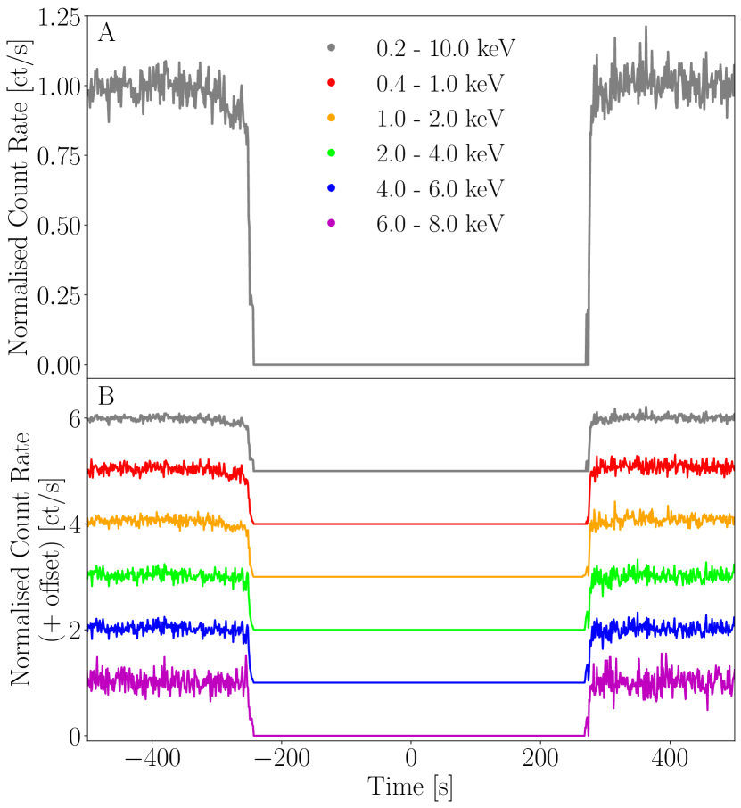
Figure 1: The folded eclipse profile of EXO 0748$-$676 in the soft-state, seen for the full energy range of XMM-Netwon ($0.2-10.0$ keV, grey) in Panels A and B, and for narrower energy ranges $0.4-1.0$ keV (red), $1.0-2.0$ keV (orange), $2.0-4.0$ keV (green), $4.0-6.0$ keV (blue) and $6.0-8.0$ keV (magenta) in Panel B. For all eclipse profiles the count rate is normalised by dividing through by the mean out-of-eclipse count rate such that the out-of-eclipse level is $1.0$ and the totality level is $0.0$. In Panel B, eclipse profiles are displayed with a vertical offset for visual clarity. These are $+0.0$ (magenta), $+1.0$ (blue), $+2.0$ (green), $+3.0$ (orange), $+4.0$ (red) and $+5.0$ (grey).

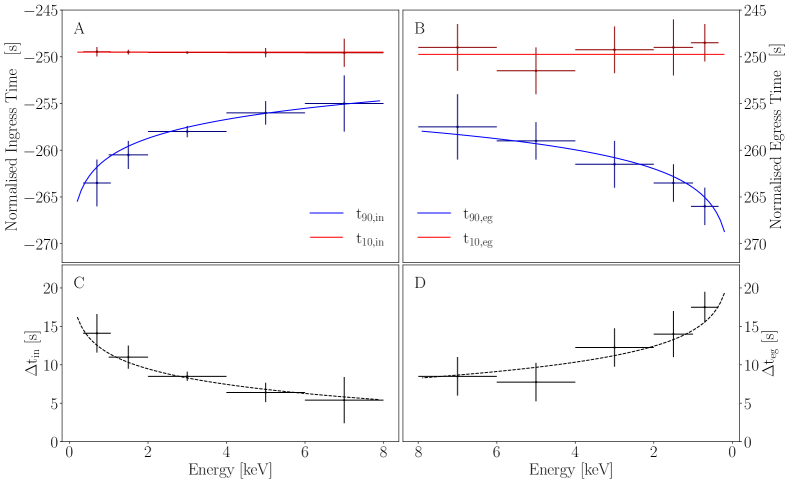
Figure 2: Measured eclipse times, $\rm{t}_{90}$ and $\rm{t}_{10}$, as functions of energy for the ingress and egress; panels A and B respectively. We define the times $\rm{t}_{90}$ and $\rm{t}_{10}$ as, respectively, the time at which the count rate is first at 90 and 10 per cent of its mean out-of-eclipse level. Times are measured from each of the eclipse profiles in Figure 1 B. Panel A: Ingress start times ($\rm{t}_{90,\rm{in}}$) increase with energy indicating that eclipses start later for higher photon energies. Ingress end times ($\rm{t}_{10,\rm{in}}$), which mark the start of totality are independent of energy. Panel B: The end of totality that marks the start of the egress ($\rm{t}_{10,\rm{eg}}$) is approximately independent of energy, but the egress ends later for softer X-rays ($\rm{t}_{90,\rm{eg}}$). Note that both axes have been reversed to aid the comparison of the egress with the ingress. Panels C and D respectively show that the ingress and egress duration increases with photon energy.

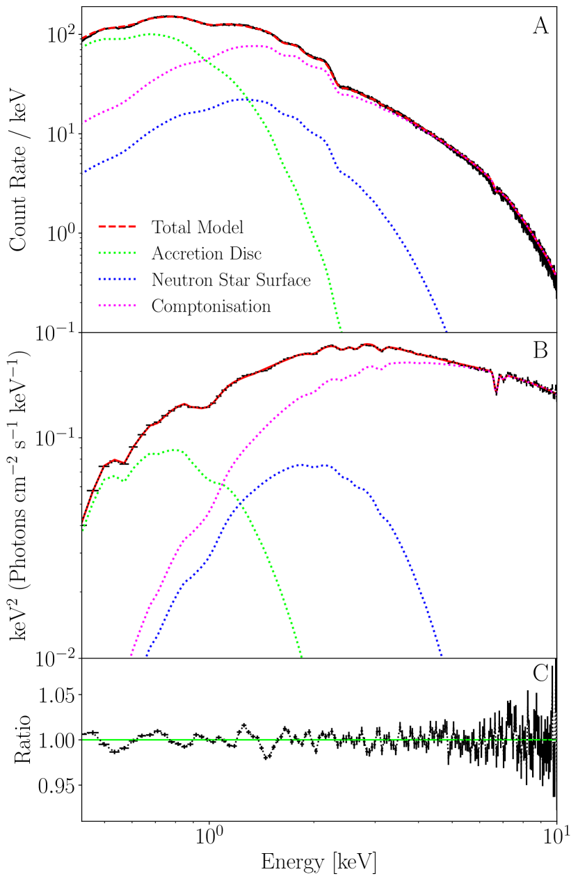
Figure 3: A fit to the time-averaged spectrum of EXO 0748$-$676 (black) using the multi-component model (red) described in Section 2.4. Also shown are the model components originating from the NS’s surface (blue), the accretion disk (green) and the thermal Comptonisation component (magenta). Model parameters are summarised in table 1 Panel A shows the best-fitting folded spectrum, panel B shows the best-fitting unfolded spectrum and panel C shows the ratio: data/folded model.

We fold the extracted light curves on the orbital period of 3.824 hours and divided through by the mean out-of-eclipse count rate. Figure 1 shows the resulting eclipse profiles that are normalised to have an out-of-eclipse count rate of $1.0$ and a totality level of $0.0$. The full $0.2-10.0$ keV band eclipse profile (Figure 1A) shows an initially gradual decline towards totality between the normalised count rate $0.8-1.0$ ct/s. This behaviour is mirrored in the egress, which shows a gradual rise out of totality between the normalised count rate $0.8-1.0$ ct/s. Figure 1B shows the eclipse profile for five energy bands, with the full band profile reproduced for comparison. To investigate the energy dependence of the eclipse profiles, we define the times $\rm{t}_{90}$ and $\rm{t}_{10}$ as those at which the count rate is first at 90 and 10 per cent of the mean out-of-eclipse level, respectively. Therefore, for the ingress, $\rm{t}_{90}$ marks the start and $\rm{t}_{10}$ the end, whereas for the egress, $\rm{t}_{10}$ marks the start and $\rm{t}_{90}$ the end. To account for stochastic variability, we define these times as the time when the average count rate first passes the desired percentage and stays past it for at least five seconds. The measured $\rm{t}_{90}$ and $\rm{t}_{10}$ values for the ingress and egress are shown in Figure 2, panels A and B respectively. For the ingress, we see that $\rm{t}_{90}$ increases with energy whereas $\rm{t}_{10}$ is approximately constant, indicating that the ingress begins later for higher photon energies, but totality starts at approximately the same time for all energies. This behaviour is mirrored in the egress: the end of totality is approximately independent of energy, but the egress ends later for softer X-rays. The ingress and egress durations, therefore, decrease with increasing photon energy. This is shown explicitly in Figures 2C and 2D. We see from these plots that the egress is longer in duration than the ingress. In the full band, the ingress duration is approximately $\rm{t_{10,in,0.2-10.0keV}-t_{90,in,0.2-10.0keV}}=15.2$ s and the egress duration is approximately $\rm{t_{90,eg,0.2-10.0keV}-t_{10,eg0.2-10.0keV}}=17.5$ s.

2.3 Interpretation

The eclipses result from the companion star passing in front of the X-ray emitting region close to the NS. To explain the extended ingress and egress duration, we consider two limiting cases: 1) an extended X-ray emitting region eclipsed by an optically thick companion star with a sharp outer boundary. 2) a point-like X-ray source eclipsed by a companion star surrounded by a layer of absorbing material with some radial density profile.

2.3.1 Extended Source with an Optically Thick Companion

In this case, the ingress duration is the time it takes for the companion to move across our view of an extended X-ray emitting region. For an edge-on, circular binary system, we can relate the radius of the assumed spherical X-ray emitting region, $r_{\rm x}$, to the ingress duration, $\Delta t_{\rm in}$, as $r_{\rm{x}}=\pi r_{\rm a}\Delta t_{\rm in}/P$, where $P$ is the orbital period and $r_{\rm a}$ is the binary separatiosn. Calculating $r_{\rm a}$ from Kepler’s law and assuming a mass ratio of $q=0.2$, we find that the observed ingress duration of $\Delta t_{\rm in}=15.2$ s requires an X-ray emitting region radius of $r_{\rm x}\approx 3500~{}{\rm km}~{}\approx 1700~{}r_{\rm g}$ for $M_{\rm ns}=1.4~{}M_{\odot}$ and $r_{\rm x}\approx 4200~{}{\rm km}~{}\approx 1200~{}r_{\rm g}$ for $M_{\rm ns}=2.4~{}M_{\odot}$; where $r_{\rm g}=GM_{\rm ns}/c^{2}$ is a gravitational radius.

In Appendix A, we show that $r_{x}$ and $q$ can be inferred as a function of binary inclination angle from the ingress duration and totality duration, under the assumption that the companion is filling its Roche-Lobe (Figure 10). The minimum inclination for which there is a solution is $i\approx 69^{\circ}$, corresponding to a mass ratio of $q=1$. For a more realistic mass ratio of $q\lesssim 0.4$, we find $i\gtrsim 73^{\circ}$. From the minimum possible inclination, we find a minimum X-ray emitting region size of $r_{x}\approx 1100~{}{\rm km}\approx 550~{}r_{g}$ for $M_{\rm ns}=1.4~{}M_{\odot}$ and $r_{x}\approx 1400~{}{\rm km}\approx 400~{}r_{g}$ for $M_{\rm ns}=2.4~{}M_{\odot}$. This large minimum source size is incompatible with, e.g., the high blackbody temperature that we measure ($kT\approx 0.5$ keV, $T\approx 5.7\times 10^{6}$ K; see Table 1), which would require a luminosity of $\sim 50$ times the Eddington limit, and for the system to be located outside of the Galaxy.

We observe the ingress and egress duration to decrease with increasing photon energy. This can be explained by the extended source model if the inner region of the source emits a harder spectrum than the outer region. In this case, the companion star starts to block the soft X-ray emitting region before it starts to cover the hard X-ray emitting region such that the hard X-ray ingress would begin after the soft X-ray ingress. However, this simple scenario predicts the hard X-ray ingress would end before the soft X-ray ingress. In contrast, we observe the start and end of totality to be roughly independent of energy, therefore this scenario cannot reproduce the energy dependence of the eclipse profiles. It also cannot reproduce the egress being longer in duration than the ingress, as we observe it to be.

2.3.2 Point Source with a Material Layer Surrounding the Companion

In the opposite limiting case, the ingress and egress occur when our view of a point-like X-ray source is blocked by a layer of absorbing material surrounding the companion star. In this picture, the surrounding material absorbs soft X-rays more efficiently than hard X-rays at the start of the ingress until the column density becomes very large at the end of the ingress, therefore, reproducing the observed energy dependence of the ingress and egress. If the absorbing material trails somewhat behind the companion star, this can explain why we observe the egress to be consistently longer than the ingress (as seen for many more eclipses: Wolff et al. 2009; Parmar et al. 1991). This is the model we adopt in this paper. We assume an X-ray point source throughout, because in this model a point source is indistinguishable from an extended source unless the source is hundreds of km across or larger.

2.4 Fit to the Time-Averaged Spectrum

Model Component	Parameter	Value	1$\sigma$  Interval
TBabs	$\rm{N}_{H}$ [1 $\times$ 1022 cm-2]	0.149	$\pm^{0.006}_{0.006}$
diskbb	T${}_{\text{in}}$ [keV]	0.218	$\pm^{0.006}_{0.006}$
bbody	$kT$ [keV]	0.491	$\pm^{0.010}_{0.012}$
NthComp	$\Gamma$	2.091	$\pm^{0.026}_{0.053}$
	$kT_{e}$ [keV]	3.469	$\pm^{0.418}_{0.310}$
Absorption lines	$E_{1}$ [keV]	6.687	$\pm^{0.009}_{0.008}$
	$E_{2}$ [keV]	7.021	$\pm^{0.030}_{0.021}$
	$E_{3}$ [keV]	2.639	$\pm^{0.021}_{0.020}$
	$E_{4}$ [keV]	3.111	$\pm^{0.018}_{0.018}$
	$E_{5}$ [keV]	3.979	$\pm^{0.229}_{0.127}$
	$\sigma_{1-5}[keV]$	0.007	$\pm^{0.005}_{0.005}$
Calibration lines	$E_{6}$ [keV]	0.990	$\pm^{0.004}_{0.004}$
	$\sigma_{6}[keV]$	0.070	$\pm^{0.002}_{0.002}$
	$E_{7}$ [keV]	2.002	$\pm^{0.016}_{0.016}$
	$\sigma_{7}$ [keV]	0.002	$\pm^{0.001}_{0.001}$
	$E_{8}$ [keV]	2.419	$\pm^{0.018}_{0.019}$
	$\sigma_{8}$ [keV]	0.016	$\pm^{0.002}_{0.001}$

Table 1: Best-fitting parameters from our fit to the time-averaged spectrum. Line energies quoted are centroid energies. Following (Ponti et al., 2014), the first 5 lines correspond to 1) a Fe XXIII-XXV K$\alpha$ blend, 2) Fe XXVI K$\alpha$, 3) S XVI K$\alpha$, 4) a S XVI K$\beta$ and Ar XVII K$\alpha$ blend, 5) A Ca XIX-XX K$\alpha$ blend. The final 3 lines account for calibration issues (see e.g. De Marco & Ponti 2016). Reduced $\chi^{2}$ is $\chi^{2}/\nu=161.57/151$. Since the duration of the ingress and egress are only$\sim 0.01\%$ of the orbital period each, and no counts are contributed during totality, the time-averaged spectrum is approximately the out-of-eclipse spectrum.

We fit the time-averaged spectrum using xspec V12.11.1 (Arnaud et al., 1996) and the model

$$\mathtt{TBabs*(diskbb+bbody+NthComp)*G}.$$ (2)

Here, TBabs accounts for absorption by the interstellar medium (we use the abundances of Wilms et al. 2000), and diskbb is a multi-temperature accretion disk spectrum. We model the spectrum from the NS surface as a blackbody (bbody) plus Comptonisation by a thermal population of electrons with temperature $kT_{\rm e}$ (NthComp; Zdziarski et al. 1996). We tie the seed photon temperature to the blackbody temperature, physically corresponding to some fraction of the NS surface blackbody photons being Compton up-scattered. Finally, G represents eight Gaussian absorption lines (gabs). The first five of these correspond to astrophysical absorption lines, originally discovered in this observation by Ponti et al. (2014). We tie the widths of these five lines but leave their centroids and strengths as free parameters. Several calibration features are evident in the $E<2.5$ keV region of the spectrum, as is common for the EPIC-pn (see e.g. De Marco & Ponti 2016). These features motivated Ponti et al. (2014) to ignore energies below $2.5$ keV. However, we wish to model the eclipse profile in soft X-rays, for which we need to extend our model for the out-of-eclipse spectrum to lower energies. We, therefore, account for the calibration features with three additional gabs components.

Figure 3 shows the total model (red) and its constituent components: the blackbody from the NS’s surface (blue), the multi-temperature blackbody from the accretion disk (green) and the thermal Comptonisation component (magenta). We achieve an acceptable fit with a reduced $\chi^{2}$ value of $\chi^{2}/\nu=161.57/151$ and a null hypothesis probability, $p=0.426$. The best-fitting parameters are reported in Table 1. Since the duration of the ingress and egress are only $\sim 0.01\%$ of the orbital period each, and no counts are contributed during totality, the time-averaged spectrum is approximately the out-of-eclipse spectrum and is subsequently used in our eclipse profile modelling.

3 Phase-Resolved Spectroscopy

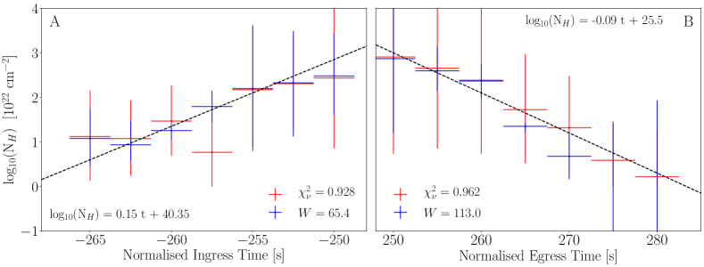
Figure 4: Hydrogen column densities as functions of time for the ingress (Panel A) and egress (Panel B), obtained by fitting our local absorption and scattering model abssca to 7 phase-resolved ingress spectra and 7 phase-resolved egress spectra. We present results obtained using two fit statistics - $\chi^{2}$ (red), quantified by $\chi^{2}/\nu$ and C-Stat (blue), quantified by the $W$ statistic. As shown, the measured Hydrogen column densities are found to be independent of the chosen fit statistic but note that C-Stat is more appropriate here because of the low count rate in several of the spectra. The eclipse times are normalised such that the centre of the eclipse occurs at $t=0$ s. In both A and B, the black dashed line shows the log-linear trend of the data. The corresponding equations for each line are given in their respective panels.

Parameter	Ingress		Egress
	$\frac{\chi^{2}}{\nu}$ = $\frac{40.8}{44}$	$W$ = 65.4	$\frac{\chi^{2}}{\nu}$ = $\frac{42.3}{44}$	$W$ = 113.0
	$p=0.77$	$p=0.67$	$p=0.54$	$p=0.47$
$\rm{f_{cov}}$	0.99  $\pm^{0.01}_{0.01}$	1.00  $\pm^{0.00}_{0.01}$	0.99  $\pm^{6\times 10^{-3}}_{0.01}$	1.00  $\pm^{0.00}_{0.01}$
$\rm{log(\xi)}$	2.81  $\pm^{0.15}_{0.55}$	3.21  $\pm^{0.08}_{0.08}$	2.57  $\pm^{0.83}_{0.19}$	2.80  $\pm^{0.42}_{0.65}$
${\rm{N}_{H}}$	13.2  $\pm^{10.8}_{9.93}$	12.0  $\pm^{0.24}_{0.21}$	808  $\pm^{80.8}_{151}$	739  $\pm^{42.6}_{46.7}$
$[10^{22}\rm{cm}^{-{2}}]$	11.9  $\pm^{7.16}_{6.84}$	8.62  $\pm^{0.42}_{0.30}$	453  $\pm^{145}_{63.4}$	394  $\pm^{3.45}_{2.83}$
	29.4  $\pm^{6.25}_{6.00}$	18.0  $\pm^{1.37}_{1.63}$	231  $\pm^{41.7}_{42.8}$	242  $\pm^{2.29}_{2.57}$
	5.85  $\pm^{6.35}_{5.85}$	62.1  $\pm^{2.25}_{2.27}$	52.8  $\pm^{17.8}_{15.8}$	22.4  $\pm^{1.20}_{1.38}$
	148  $\pm^{28.6}_{24.1}$	158  $\pm^{24.6}_{21.6}$	20.8  $\pm^{14.4}_{12.9}$	4.75  $\pm^{0.30}_{0.32}$
	203  $\pm^{10.6}_{10.4}$	212  $\pm^{14.7}_{16.0}$	3.86  $\pm^{7.58}_{3.86}$	$10^{-9}$  $\pm{10^{-10}}$
	272  $\pm^{54.7}_{37.8}$	303  $\pm^{8.87}_{7.37}$	1.66  $\pm^{10.6}_{1.66}$	$10^{-8}$  $\pm{10^{-10}}$
$n_{\rm{H}}$		0.56 $\pm^{0.08}_{0.07}$		0.56 $\pm^{0.08}_{0.07}$
$[10^{22}\rm{cm}^{-{2}}]$
$\alpha$		2.68 $\pm^{0.14}_{0.15}$		2.68 $\pm^{0.14}_{0.15}$

Table 2: Best fitting parameters obtained from fitting our local absorption and scattering model abbsca to the phase-resolved spectra of the ingress and egress. We present results obtained using two fit statistics - $\chi^{2}$, quantified by $\chi^{2}/\nu$ and C-Stat, quantified by the $W$ statistic. Their values are given in the first and second columns respectively for both the ingress and egress, with corresponding null hypothesis probabilities below. The model parameters are found to be consistent between the two fit statistics, but C-Stat is more appropriate because of the low count rate in several of the spectra. Here, $\chi^{2}_{\nu}$ provides a simple way to understand the goodness of fit. The rows are covering fraction, $\rm{f_{cov}}$, ionisation parameter, $\rm{log(\xi)}$, and column density for each time bin, $\rm{N_{H}}$. The column densities are listed chronologically. The bottom two rows detail the best-fitting parameters for the background spectral model, TBabs*po, which are the equivalent hydrogen column, $n_{\rm{H}}$ and the power-law index, $\alpha$. All errors are $1\sigma$ and the same background spectral fit was applied to both the ingress and egress.

To diagnose the nature of the absorbing material around the companion star, we fit the phase-resolved spectra of the ingress and egress with a model that accounts for the absorption and scattering of X-ray photons by the material.

3.1 Spectral Model

We define a local xspec model called abssca in which the total transmitted specific intensity $I_{\rm E}$ relates to the out-of-eclipse specific intensity $I^{0}_{\rm E}$ as

$$I_{\rm E}=I^{0}_{\rm E}\bigg{\{}\rm{f}_{\rm cov}\exp\{-N_{\rm H}[\sigma(\textit{E})+(n_{\rm e}/n_{\rm H})\sigma_{\rm T}]\}+1-\rm{f}_{\rm cov}\bigg{\}},$$ (3)

where $\rm{f}_{\rm cov}$ is the covering fraction of the absorbing material around the companion star (a fraction $\rm{f}_{\rm cov}$ of the incident photons have interactions and the rest pass straight through), $\rm{N}_{H}$ is the hydrogen column density, $\sigma(E)$ is the absorption cross-section, $\sigma_{\rm T}$ is the Thomson electron scattering cross-section, and the density ratio $\rm{n_{e}/n_{H}}$ is the ratio of free electrons to hydrogen nuclei in the medium (i.e. the electron column density is $\rm{N}_{e}=\rm{N}_{H}~{}n_{e}/n_{H}$). We use the xspec model zxipcf (Miller et al., 2006) to calculate the absorption cross-section, which depends on the ionisation parameter $\xi$.

In addition to being absorbed by the material surrounding the companion, photons can be scattered by the material layer out of the line of sight. Also, photons can be scattered into the line of sight, but this effect is negligible in our case because the stellar absorber subtends a small solid angle according to the X-ray source. This is in contrast to a commonly considered scenario of a spherical shell of absorbing material surrounding a central source, in which case photons scattered into the line of sight will exactly cancel those scattered out of the line of sight. For $\xi\lesssim 100~{}{\rm erg}~{}{\rm cm}~{}{\rm s}^{-1}$, the absorption cross-section dominates over the scattering cross-section except for $E\gtrsim 10$ keV. For $\xi\gtrsim 100~{}{\rm erg}~{}{\rm cm}~{}{\rm s}^{-1}$, $\sigma(E)$ additionally dips below $\sigma_{\rm T}$ for $E\lesssim 0.5$ keV and $E\sim 7$ keV (see e.g. Figure 1.21 of Done 2010). The density ratio $\rm{n_{e}/n_{H}}$ can, in principle, be calculated from the ionisation state and relative elemental abundances of the gas, such that $\rm{n_{e}/n_{H}}$ increases with $\xi$. For instance, a pure hydrogen gas would have $\rm{n_{e}/n_{H}}$ in the range zero to unity, whereas the presence of heavier elements makes $\rm{n_{e}/n_{H}}>1$ possible. Here we simply fix $\rm{n_{e}/n_{H}}=1$ throughout. This is appropriate for larger values of $\xi$, but not for smaller values. However, for smaller values of $\xi$, $\sigma(E)\gg\sigma_{\rm T}$ for the entire XMM-Newton band pass and therefore scattering is negligible, rendering the model insensitive to $\rm{n_{e}/n_{H}}$. We additionally fix the redshift to $z=0$.

3.2 Results

We extract phase-resolved spectra for the ingress and egress from the folded eclipse profiles in 6 energy bands: $0.2-0.5$ keV , $0.5-1.0$ keV, $1.0-2.0$ keV, $2.0-4.0$ keV, $4.0-6.0$ keV and $6.0-8.0$ keV (which were calculated following the procedure described in Section 2.2). Spectra are extracted using 2.5 second and 5.0 second time bins, respectively, for the ingress and egress, covering time ranges of t $=-267.5$s to t $=-250.0$s and t $=247.5$s to t $=282.5$s, producing a total of 14 spectra (seven for the ingress and seven for the egress). The time ranges are defined to ensure we fully encapsulate the times in which the absorbing material is influencing the eclipses, and to account for the observed asymmetry in the eclipse profiles.

Because of the asymmetry in the eclipses, we allow the ingress and egress to have different values of covering fraction ($\rm{f}_{\rm cov}$), ionisation parameter ($\xi$) and column density ($\rm{N}_{H}$). We initially allow the covering fractions and ionisation parameters to be free for each spectrum, finding their values to be approximately constant across the sets of ingress and egress spectra. We, therefore, tie the covering fractions and ionisation parameters for the sets of ingress and egress spectra (such that it is constant in both sets), but the column density remains a free parameter for each spectrum. The xspec fit results are shown in Table 2, where the column densities are listed chronologically. We find that $\log(\rm{N}_{H})$ increases linearly with time during the ingress and decreases linearly with time in the egress, as shown by the dashed black lines in Figure 4. The column density is found to change by several orders of magnitude over a short time, suggesting the absorbing material possesses a steep density profile.

Note that two fit statistics are considered here. Due to the low count rate in several of the spectra, C-Stat is more appropriate than $\chi^{2}$. Within xspec, this requires a background spectrum and model to be defined because the difference between two Poisson variables is not another Poisson variable. Therefore, instead of subtracting the background from the source, the combined likelihood for the source and background are found and quantified with the W-Statistic (see Arnaud, Dorman & Gordon 1996 Appendix B for further details). The background spectrum is simply the totality spectrum and is well-modelled by an ISM absorption and power-law model: TBabs*po. We present best-fitting model parameters for the ingress and egress spectra using both fit statistics (C-Stat and $\chi^{2}$) in Table 2, to show that the best-fitting parameters are independent of the chosen fit-statistic. Table 2 also details the best-fitting parameters for the background spectral fit which was used in both the ingress and egress spectral fits.

3.3 Inferring the Density Profile

We model the companion star as spherically symmetric with radial hydrogen number density profile $n_{\star}(r)$. The photospheric radius of the star is $R_{\rm cs}$, such that $n_{\star}(r)$ in the region $r<R_{\rm cs}$ is large enough for the optical depth to be effectively infinite. Totality therefore occurs whenever the projected separation on the image plane between the centre of the companion star and the X-ray point source is less than $R_{\rm cs}$. Defining the impact parameter, $b(t)$ as this projected separation in units of $R_{\rm cs}$ means that totality occurs for all times when $b(t)\leq 1$. For $b(t)>1$, the hydrogen column density for a sight-line through the surrounding material is:

$$\rm{N}_{H}(t)=\int_{-\infty}^{+\infty}n_{\star}(r)ds,$$ (4)

where $s$ is the distance a ray has travelled along a given sight line. Here $s=0$ is defined as when the ray passes closest to the centre of the companion star. Therefore, a ray travelling along a sight line that starts behind the star and points towards the observer extends from $s=-\infty$ to $s=+\infty$. Defining $x\equiv r/R_{\rm cs}$ as distance in units of the companion star radius, it can be shown that $(s/R_{\rm cs})^{2}=x^{2}-b^{2}$, and we can therefore re-write the above integral as

$$\rm{N}_{H}(t)=2N_{H,0}\int_{b(t)}^{x_{\rm out}}n(x)\frac{x}{\sqrt{x^{2}-b^{2}(t)}}dx,$$ (5)

where $n(x)\equiv n_{\star}(r)/n_{0}$ such that $n_{0}=n_{\star}(r=R_{\rm cs})$ and $N_{H,0}=R_{\rm cs}n_{0}$ is the column density of a sight-line of length $R_{\rm cs}$ through material with constant density $n_{0}$. Here, $x_{\rm out}$ is the outermost radius of the absorbing medium with non-negligible density.

For a perfectly circular binary system with orbital period, $P$, separation, $r_{\rm a}$, and inclination angle to the observer, $i$, we can write the impact parameter as:

$$b(\phi)=\frac{r_{a}}{R_{\rm cs}}\sqrt{1-\sin^{2}i~{}\cos^{2}\phi},$$ (6)

and the orbital phase as $\phi=(2\pi/P)(t-t_{0})$, where $t_{0}$ is the time at the centre of totality. From this, we can show that the duration of totality, $t_{e}$, obeys

$$\left(\frac{R_{\rm cs}}{r_{\rm a}}\right)^{2}=1-\cos^{2}\left(\frac{\pi\ t_{e}}{P}\right)~{}\sin^{2}i.$$ (7)

Assuming the companion star is filling its Roche Lobe, the ratio $R_{\rm cs}/r_{\rm a}$ is (Horne, 1985; Ratti et al., 2012):

$$\frac{R_{\rm cs}}{r_{a}}=h(q)=\frac{0.49q^{2/3}}{0.6q^{2/3}+\ln(1+q^{1/3})},$$ (8)

where $q=M_{\rm cs}/M_{\rm ns}$. We can then calculate the inclination angle from Equations 7 and 8 as:

$$\sin i=\frac{\sqrt{1-h^{2}(q)}}{\cos(\pi t_{e}/P)}.$$ (9)

Therefore, for known $t_{\rm e}$, $P$ and $t_{0}$, the only model parameter required to calculate $b(t)$ is $q$. The column density $\rm{N}_{H}(t)$ can be calculated from an assumed radial density function, $n(x)$, with $q$ as the only other model parameter.

We trial a number of density profiles, the first is a power law:

$$\centering n(x)=x^{-m}.\@add@centering$$ (10)

Setting $m=2$ corresponds to a stellar wind with constant velocity. The companion star in EXO 0748$-$676 is a low mass M-dwarf star (Parmar et al., 1986) that would typically be expected to only drive a weak solar-like wind with a mass-loss rate of the order of $10^{-13}M_{\odot}$ yr^-1 or less (e.g., Wargelin & Drake, 2002). Such a wind is too low-density to yield significant absorption at X-ray wavelengths: a wind velocity of 500 km s^-1, for example, corresponds to a particle density at the base of the wind of $6\times 10^{6}$ cm^-3 for the typical M-dwarf radius of $R_{cs}=0.43R_{\odot}$, and a column density through the wind of $2\times 10^{17}$ cm^-2. In this case, however, a much denser wind could be driven by irradiation from the NS and accretion flow.

We trial power-law indices of $m=-2,\ m=0,\ m=2\ \rm{and}\ m=10$. For each index, we also explore mass ratios of $q=0.05,\ q=0.2\ \rm{and}\ q=0.4$, corresponding to inclination angles of $i=82.8,\ i=76.9\ \rm{and}\ i=73.6$ degrees respectively. Here, $q=0.05$ translates roughly to the canonical NS mass, $1.4M_{\odot}$. As seen in the top row of Figure 5, the power-law density profile results in an $\rm{N}_{H}(t)$ that overwhelmingly disagrees with observations, for both the ingress and egress. We find higher values of $m$ and $q$ to be the most consistent with $m=10$ and $q=0.4$ providing $\chi^{2}/\nu=464.2/44$ for the ingress and $\chi^{2}/\nu=332.4/44$ for the egress. The null hypothesis probabilities for both are of the order $10^{-30}$. We conclude that the asymptotic nature of the power-law function trialled will not easily reproduce the observed, steep $N_{\rm{H}}(t)$.

The data require a density profile that drops off more steeply with radius rather than a constant velocity wind. We therefore consider a density profile corresponding to an accelerating wind (Puls et al., 2008):

$$n(x)=x^{-2}~{}(1-x^{-1})^{-\beta},$$ (11)

where $\beta$ is a parameter that describes the acceleration. In this case, the constant $N_{\rm H,0}$ from Equation (5) is related to the mass loss rate of the wind, $\dot{M}_{\rm out}$, as:

$$N_{H,0}=\frac{\dot{M}_{\rm out}}{4\pi\bar{m}\sqrt{GM_{\rm cs}R_{\rm cs}}},$$ (12)

where $\bar{m}$ is the mean molecular weight of the wind material. Equation (11) is typically applied to massive stars for which the wind is driven by the radiation of the star itself. Puls et al. (2008) quote $\beta\leq 1.0$ for an OB star, however, we require much higher values to obtain consistency with the data. With a parameter combination of $\beta=3.0$ and $q=0.2$, $\chi^{2}/\nu=85.1/44$, while a parameter combination of $\beta=5.0$ and $q=0.4$ gives $\chi^{2}/\nu=64.9/44$ for the ingress. For the egress these are, respectively, $\chi^{2}/\nu=140.1/44$ and $\chi^{2}/\nu=74.9/44$. Panels C and D of Figure 5 show this consistency for parameter combinations of $\beta=2.0,\ q=0.05,\ \beta=3.0,\ q=0.2,\ \rm{and}\ \beta=5.0,\ q=0.4$, with the latter providing the best overall agreement. This could indicate that there is very fast-moving material surrounding the companion, or that this, an M-dwarf star within an X-ray binary, is an inappropriate context for this functional form (Equation 11), especially since it is usually applied to hot, massive stars.

We consider the possibility that the absorbing material may behave less like a stellar wind and more like an extended atmosphere. Therefore we trial a Gaussian density profile characterised by the fractional width of the material layer, $\Delta$, which is a steeper function of distance, and therefore should be more consistent with the observed $\rm{N}_{H}(t)$. We express this form of density profile as:

$$n(x)=\exp\left[-\frac{(x-1)^{2}}{2\Delta^{2}}\right],$$ (13)

and try values of $\Delta=0.008,\ \Delta=0.005\ \rm{and}\ \Delta=0.003$ for the set of mass ratios detailed above. As seen in Panels E and F of Figure 5, we achieve better agreement with the observed $\rm{N}_{H}(t)$, particularly for the ingress, where the parameter combination $\Delta=0.003$ and $q=0.4$ gives the most consistent result $\chi^{2}/\nu=64.3/44$. The eclipse timings (see Section 2.2) suggested that there might be material trailing behind the companion star as it orbits, therefore, it is unsurprising that a larger fractional width, $\Delta=0.008$, is most consistent with the egress data ($\chi^{2}/\nu=64.4/44$, with $q=0.05$), further supporting the presence of an asymmetric eclipse.

We additionally trial an exponential density profile for the material:

$$n(x)=\exp\left[\frac{1-x}{h}\right],$$ (14)

where $h$ is the scale height of the material in units of $R_{\rm cs}$. For the ingress we consider $h=0.004$, $h=0.002$ and $h=0.001$, and for the egress $h=0.009$, $h=0.004$ and $h=0.003$. It is clear that the $\rm{N}_{H}(t)$ functions predicted from this density profile provide the best description of the data, as seen in Panels G and H of Figure 5. For the ingress, the most consistent parameter combination is $h=0.002,q=0.2$ giving $\chi^{2}/\nu=52.0/44$, and for the egress the most consistent parameter combination is $h=0.004,q=0.2$ giving $\chi^{2}/\nu=44.6/44$.

Overall, the exponential radial density profile (Equation 14) is most consistent with the observed $\rm{N}_{H}(t)$, but using the results from all density profiles, we can infer some properties of the absorbing material. The Gaussian density profile requires small fractional widths ($\Delta$), the exponential profile requires small scale heights ($h$), and the accelerating profile requires high values for $\beta$, indicating that the density of material must drop off quickly with distance from the companion star’s surface in all three cases. The Gaussian and exponential profiles also highlight the asymmetry of the eclipse profiles. When using the Gaussian density profile, the parameter combination $\Delta=0.003$ and $q=0.4$ yields $\chi^{2}/\nu=64.3/44$ for the ingress, but yields a notably worse fit of $\chi^{2}/\nu=277/44$ for the egress. Similarly, when using the exponential density profile with $q=0.2$, a scale height of $h=0.004$ is needed for the egress to produce $\chi^{2}/\nu=44.6/44$, while $h=0.002$ for the ingress is required to give the comparable $\chi^{2}/\nu=52.0/44$. These results imply that more material is present in our line-of-sight during the egress than the ingress thus we consider a scenario in which the absorbing material trails behind the companion as it orbits, perhaps similar to a comet-tail. This could explain the 2.3 s asymmetry we observed in the folded eclipse profiles (Section 2.2). The phase-resolved spectral fits also provide useful insights. The ingress and egress both require high ionisation parameters, with the ingress being slightly more ionised than the egress. Such levels of ionisation could be driven by irradiation from the NS itself, perhaps being collisionally ionised by a pulsar wind. The difference in ionisation and covering fraction are likely due to the orbital motion of the binary.

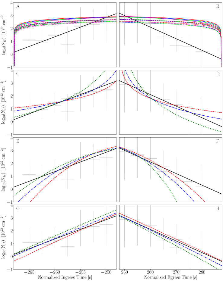
Figure 5: Panels A-H: Hydrogen column density of the absorbing material as a function of time during the ingress and egress. Measured $N_{\rm H}$ values are shown in grey with a log-linear best-fit function in black. Panels A and B assume the power law density profile (Equation 10). We use mass ratio q = 0.05 (solid), q = 0.2 (dashed) and q = 0.4 (dot-dashed); which correspond to $i$ = 82.8 , $i$ = 76.9 and $i$ = 73.6 degrees respectively. We explore a power-law index of m = –2 (red), m = 0 (blue), m = 2 (green) and m = 10 (magenta). Panels C and D assume the accelerating wind profile (Equation 11) with parameter combinations of $q=0.05,\beta=2.0$ (red), $q=0.2,\beta=3.0$(blue) and $q=0.4,\beta=5.0$ (green). Panels E and F assume the Gaussian density profile (Equation 13). We use mass ratio and fractional width parameter combinations of $q=0.05,\Delta=0.008$ (red), $q=0.2,\Delta=0.004$ (blue) and $q=0.4,\Delta=0.003$ (green) for the ingress and combinations of $q=0.05,\Delta=0.008$ (red), $q=0.2,\Delta=0.004$ (blue) and $q=0.4,\Delta=0.003$ (green) for the egress. Panels G and H assume the exponential density profile (Equation 14). We use mass ratio and scale height parameter combinations of $q=0.05,h=0.004$ (red), $q=0.2,h=0.002$ (blue) and $q=0.4,h=0.001$ (green) for the ingress and combinations of $q=0.05,h=0.009$ (red), $q=0.2,h=0.004$ (blue) and $q=0.4,h=0.003$ (green) for the egress. Panels C-H: We trial $q=0.05,q=0.2$ and $q=0.4$ for each value of $\beta$, $\Delta$ and $h$ but only plot three in each panel for visual clarity.

4 Eclipse Mapping

4.1 Eclipse profile model

We represent the out-of-eclipse spectrum with the spectral model described in Section 2.4 with the parameters fixed to their best fitting values (Table 1). We then calculate the time-dependent specific photon flux, $S(E,t)$, by multiplying the out-of-eclipse spectrum, $S_{0}(E)$, by an energy dependent transmission factor given by our absorption and scattering model abssca, which depends on ionisation parameter, covering fraction and hydrogen column density. The ionisation parameter and covering fraction are left as free model parameters, with the values for the ingress ($t<t_{0}$), $\xi_{\rm in}$ and $\rm{f}_{\rm cov,in}$, allowed to be different from the corresponding egress ($t>t_{0}$) values, $\xi_{\rm eg}$ and $\rm{f}_{\rm cov,eg}$. We calculate the column density as a function of time, $\rm{N}_{H}(t)$, from Equation (5), which depends on mass ratio, $q$, the surface column density, $N_{H,0}$, and an assumed parameterisation of the stellar radial density profile, $n(x)$. We trial all four forms of $n(x)$ considered in Section 3.3: 1) a power law with index $m$ (Equation 10), 2) an accelerating wind with acceleration parameter $\beta$ (Equation 11), 3) a Gaussian with fractional width $\Delta$ (Equation 13), and 4) an exponential form with scale height $h$. We allow $N_{H,0}$ and each of the $n(x)$ parameters ($m$, $\beta$, $\Delta$ or $h$, depending on the model being used) to take different values for ingress and egress. We only compute the integral in Equation (5) for orbital phases with $1\leq b(\phi)\geq x_{\rm out}$, whereas $b(\phi)<1$ corresponds to totality and $b(\phi)>x_{\rm out}$ to out-of-eclipse. In order to demonstrate the need for a layer of material around the companion star, we additionally trial a model that transitions sharply from out-of-eclipse for $b(\phi)>1$ to totality for $b(\phi)<1$. We fix the orbital period to $P=3.824$ hrs and leave the totality duration $t_{e}$ as a free model parameter.

The time-dependent count rate in the XMM-Newton energy range consisting of channels $I_{1}$ to $I_{2}$ is

$$C(I_{1},I_{2},t)=\int_{0}^{\infty}~{}A_{\rm eff}(E,I_{,}I_{2})~{}S(E,t)~{}dE,$$ (15)

where

$$A_{\rm eff}(E,I_{2},I_{2})=\sum_{I=I_{1}}^{I_{2}}~{}R_{D}(I,E),$$ (16)

is the effective area of the combined instrument channels $I_{1}$ to $I_{2}$ (analogous to a photometry filter), and $R_{D}(I,E)$ – the instrument response – is the effective area of channel $I$ (see Rapisarda et al. 2016). In practice, the instrument response is quantised into the response matrix stored in the rmf and arf files, which we read into our model. For convenience when fitting, both the data and model in each energy band are divided by the mean out-of-eclipse count rate such that the out-of-eclipse count rate equals $1.0$ and the totality level is $0.0$.

4.2 Results

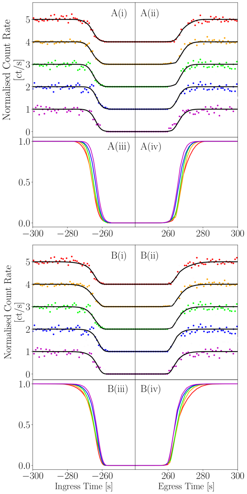
Figure 6: Eclipse profiles resulting from fitting the eclipses of EXO 0748$-$676 in five energy bands to the eclipse profile model assuming the Gaussian density profile (panels A(i)$-$A(iv) ) and the exponential density profile (panels B(i)$-$B(iv) ). Colours are represent the 5 narrow energy bands used in our modelling and are consistent with Figure 1. In each set of four panels, i and ii show the resulting fits to each individual energy band, each with a vertical offsets for visual clarity. These are $+0.0$ (magenta), $+1.0$ (blue), $+2.0$ (green), $+3.0$ (orange) and $+4.0$ (red). In each set of four panels, iii and iv show the resulting model in each energy band without a vertical offset to clearly show the energy dependent behaviour of the best-fitting eclipse profiles. Fit statistics achieved are $\chi^{2}/\nu=822.95/816$ and $\chi^{2}/\nu=816.01/816$ for the Gaussian (A) and exponential (B) models respectively.

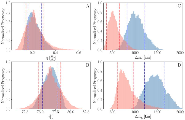
Figure 7: Distributions of mass ratio (A), inclination angle (B), width of absorbing material during ingress (C) and width of the absorbing material during egress (D), from the eclipse profile model. The distributions are obtained through a Markov Chain Monte Carlo simulation with 256 walkers, 307200 steps and a burn-in of 92160 steps assuming the Gaussian density profile (blue) and the exponential density profile (red). Corresponding $1\sigma$ confidence intervals are shown by blue and red dashed lines respectively.

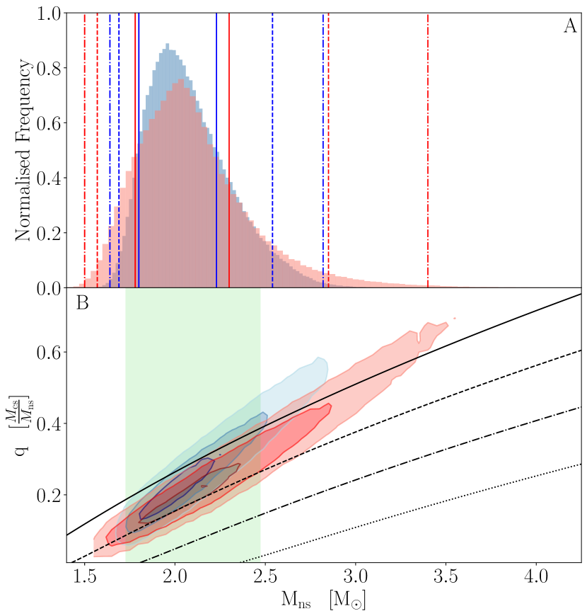
Figure 8: Panel A: Distributions of $M_{\rm{ns}}$ assuming the Gaussian (blue) and exponential (red) density profiles within the eclipse profile model. Distributions are obtained through a Markov Chain Monte Carlo simulation with a length of 307200, 256 walkers and a burn-in length of 92160 steps. Vertical lines show $1\sigma$ (solid), $2\sigma$ (dashed) and $3\sigma$ (dot-dashed) contours in blue and red, for the Gaussian and exponential density profiles respectively, which peak at $2.01M_{\odot}$ and $2.02M_{\odot}$. Panel B: Comparison between our measurements of $M_{\rm{ns}}$ assuming the Gaussian density profile (blue) and the exponential density profile (red), and the measurement from Özel 2006 (green). Dark, mid and light shades of blue and red correspond to $1$, $2$ and $3\sigma$ contours respectively for the Gaussian and exponential density models. Black lines show the relationship between, $M_{\rm{ns}}$ and $q$, for K-corrections of 1.0 (solid), 0.9 (dashed), 0.8 (dot-dashed) and 0.7 (dotted). K-corrections closer to unity yield a lower NS mass.

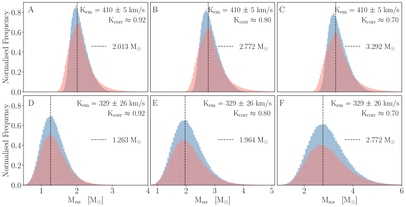
Figure 9: Distributions of $M_{\rm{ns}}$ assuming the Gaussian (blue) and exponential (red) density profiles within the eclipse profile model calculated using a different combination of $K_{\rm em}$ and K-Correction (as labelled). Also shown is a black dashed line corresponding to the peak-posterior NS mass. The K-correction in A and D corresponds to the most conservative value calculated using the mass-ratio dependent relation of Munoz-Darias et al. (2005) (Equation 18) for our best fitting value $q=0.222$. Column 2 (B and E) and column 3 (C and F) assume the reasonable K-corrections of 0.8 and 0.7 respectively. Emission lines considered are H_α, $K_{\rm em}=$410 $\pm$ 5 km/s (Bassa et al., 2009) and CIII$-$NIII blend, $K_{\rm em}=$329 $\pm$ 26 km/s (Mikles & Hynes, 2012). We see that the peak-posterior is above the canonical NS mass unless we discard the H_α measurement and employ the maximum (closest to unity) possible K-correction (panel D).

Using xspec v12.1.1, we simultaneously fit the eclipse profiles of EXO 0748$-$676 in the five narrow energy bands presented in Figure 1B. We ignore the majority of the phase bins corresponding to out-of-eclipse and totality, leaving only a small number of bins surrounding the ingress and egress. This ensures the best-fitting parameters and statistics refer to the portions of the eclipse profiles that contain the energy-dependent behaviour. Due to the abundance of observations of EXO 0748$-$676, the eclipse duration, $t_{e}$ of $\sim 500$ s is well-known, but is also observed to vary (Wolff et al., 2009; Parmar et al., 1991). Therefore, we apply a Bayesian prior on $t_{\rm e}$ assuming a Gaussian peaking at $500$s with a width of $5$s.

We first trial our eclipse profile model with no absorbing material surrounding the companion. This model simply invokes a sharp transition between out of eclipse and totality. This model produces a poor fit to the observed eclipse profiles (see row 1 of Table 3), demonstrating the need for the layer of absorbing material. We further trial the four density profiles presented in Equations 10 - 14. Table 3 compares the resulting fit statistics from our eclipse model for each density profile. As anticipated, the power-law density profile, with reasonable power-law indices of $m=2$ and $m=10$, are unable to describe the data, respectively yielding $\chi^{2}/\nu=17700/818$ and $\chi^{2}/\nu=15600/818$. Interestingly, if the power-law index is allowed to vary during the fits and be different for the ingress and egress, they rise to the high values of $m_{\rm{in}}\approx 410.0$ and $m_{\rm{eg}}\approx 760.0$. At such high values of $m$, the power-law function behaves similarly to the exponential function (Equation 14), so based on our previous inferences, it is not surprising that these values yield a much lower fit statistic ($\chi^{2}/\nu=1352/816$). As such high indices are nonphysical, we subsequently discard the power-law density profile. The remaining three profiles yield reasonable fits to the eclipse profiles, as alluded to by the phase-resolved spectroscopy. However, we discard the accelerating wind profile because 1) the associated $\chi^{2}_{\nu}=1.288$ is notably higher than assuming the Gaussian ($\chi^{2}_{\nu}=1.009$) or exponential ($\chi^{2}_{\nu}=1.000$) density profiles and 2) the associated null-hypothesis probability, $p=10^{-39}$, indicates that this model does not reproduce the data.

The eclipse profile model assuming the Gaussian ($\chi^{2}/\nu=822.95/816$) or exponential ($\chi^{2}/\nu=816.01/816$) density profiles are difficult to separate statistically, therefore, we consider both profiles going forward. The resulting eclipse profiles are shown in Figure 6, where panels A(i)$-$A(iv) assume the Gaussian density profile and panels B(i)$-$B(iv) assume an exponential density profile. Associated best-fitting parameters can be found in Table 4, with $1\sigma$ confidence intervals obtained through a Markov-Chain Monte Carlo (MCMC) simulation (see Appendix C for full details). The best-fitting parameters from either profile lead to a similar inference regarding the absorbing material – the fractional widths and scale heights are both small, confirming that the material doesn’t extend far out from the star’s surface. Both profiles show asymmetry here, with larger fractional widths and scale heights for the egress than for the ingress. When assuming the exponential density profile, our fits suggest there is $\sim 20\%$ more material in the egress than the ingress while assuming the Gaussian density profile increases this to $\sim 40\%$. This further supports the hypothesis that some material is trailing behind the companion as it orbits. We find consistent ionisation parameters between the two density profiles, with both profiles finding the ingress to be more ionised than the egress, thus suggesting an incident wind or irradiation from the NS more strongly affects the ingress side of the star. The two models show variations in covering fraction, with the Gaussian model indicating the ingress side of the star is less covered by absorbing material than the egress side of the star, although the larger errors associated with $\rm{f_{cov,in}}$ mean that the two sides could have similar coverings. In comparison, the exponential model shows the covering fractions to be consistent between the two sides of the star. The best-fitting mass ratio, $q$, and inclination angle, $i$, are found to be independent of the assumed radial density profile; we, therefore, have increased confidence in these values and our subsequent inference of the NS mass. Nonetheless, the energy-dependent eclipse timings strongly depend on the chosen density profile, so it is necessary to understand the density of the material to model the features of the eclipses caused by absorption. When comparing the eclipses modelled with the Gaussian density profile to the eclipses modelled with the exponential density profile (i.e. comparing panels A(iii) and A(iv) with panels B(iii) and B(iv) of Figure 6), we see the energy bands are more dispersed at the start ($\rm{t_{10,in}}$) and end ($\rm{t_{10,eg}}$) of totality when modelled with the Gaussian density profile. As a result, the Gaussian model does not capture the energy independence of the observed $\rm{t_{10}}$ times as well as the exponential model. Both models are capable of reproducing the observed $\rm{t_{90,in}}$ and $\rm{t_{90,eg}}$.

Density Profile	Parameter(s)	$\chi^{2}$	$\nu$	$\chi^{2}_{\nu}$	$p$
No Material	-	4546.74	818	5.56	$10^{-256}$
Power-law	m = 2.00 *	17700	818	21.61
	m = 10.0 *	15400	818	18.81
	$\rm{m_{in}}$  = 413.6	1352.1	816	1.65	$10^{-167}$
	$\rm{m_{eg}}$  = 764.9
Accelerating	$\beta_{\rm{in}}$ = 5.48	1050.6	816	1.288	$10^{-39}$
	$\beta_{\rm{eg}}$ = 6.20
Gaussian	$\Delta_{\rm{in}}$ = 0.0035	822.95	816	1.009	0.581
	$\Delta_{\rm{eg}}$ = 0.0047
Exponential	$\rm{h}_{\rm{in}}$ = 0.0023	816.01	816	1.000	0.610
	$\rm{h}_{\rm{eg}}$ = 0.0027

Table 3: Fit statistics and characteristic density profile parameters obtained from fitting the eclipse mapping model simultaneously to eclipses profiles of EXO 0748$-$676 in five energy bands, for each assumed density profile. From left to right: the assumed density profile of the absorbing material, key parameters governing the density profile, chi-squared, number of degrees-of-freedom, reduced chi-squared The key density parameters are power-law index, $m$, acceleration parameter, $\beta$, fractional width of the material, $\Delta$ and scale height, $h$, for the power-law, accelerating, Gaussian and exponential density profiles respectively. * Parameter fixed for the duration of the fit.

Parameter	Gaussian Density Profile	Derived Values
$t_{\rm e}$	503.21 $\pm^{1.62}_{1.48}$	$i=76.52\pm^{1.37}_{1.13}$
$q$	0.221 $\pm^{0.057}_{0.057}$	$M_{\rm{ns}}=2.01\pm^{0.22}_{0.21}$
$N_{H0,\rm{in}}$	2364.32 $\pm_{666.8}^{682.7}$
$N_{H0,\rm{eg}}$	4842.15 $\pm_{543.3}^{506.2}$
$\log(\xi)_{\rm{in}}$	3.49 $\pm_{0.084}^{0.460}$
$\log(\xi)_{\rm{eg}}$	2.82 $\pm_{0.043}^{0.009}$
$\rm{f_{cov,in}}$	0.897 $\pm_{0.062}^{0.064}$
$\rm{f_{cov,eg}}$	0.995 $\pm_{0.002}^{0.002}$
$\Delta_{\rm{in}}$	0.0035 $\pm_{0.0006}^{0.0006}$	$\Delta x=1033\pm^{194}_{186}$ km
$\Delta_{\rm{eg}}$	0.0049 $\pm_{0.0007}^{0.0008}$	$\Delta x=1446\pm^{216}_{236}$ km
Parameter	Exponential Density Profile	Derived Values
$t_{e}$	504.11 $\pm_{0.62}^{0.56}$	$i=76.47\pm^{1.89}_{1.79}$
$q$	0.222 $\pm_{0.075}^{0.070}$	$M_{\rm{ns}}=2.02\pm^{0.29}_{0.27}$
$N_{H0,\rm{in}}$	3819.7 $\pm_{1040.2}^{1023.9}$
$N_{H0,\rm{eg}}$	4320.3 $\pm_{972.4}^{881.3}$
$\log(\xi)_{\rm{in}}$	3.30 $\pm_{0.013}^{0.349}$
$\log(\xi)_{\rm{eg}}$	2.76 $\pm_{0.125}^{0.081}$
$\rm{f_{cov,in}}$	0.998 $\pm_{0.001}^{0.002}$
$\rm{f_{cov,eg}}$	0.996 $\pm_{0.009}^{0.005}$
$\rm{h_{in}}$	0.0023 $\pm_{0.0001}^{0.0012}$	$\Delta x=679\pm^{222}_{107}$ km
$\rm{h_{eg}}$	0.0027 $\pm_{0.0009}^{0.0004}$	$\Delta x=797\pm^{104}_{251}$ km

Table 4: Best fitting parameters obtained when fitting the eclipse mapping model simultaneously to the eclipse profiles of EXO 0748$-$676 in five energy bands. We implement both the Gaussian (top table) and exponential (bottom table) density profiles for the absorbing material around the companion star. From top to bottom the model parameters are totality duration, mass ratio, surface column density for the ingress and egress, ionisation parameter for the ingress and egress, covering fraction for the ingress and egress. The final two parameters are the fractional widths of the surrounding material layer for the ingress and egress in the case of the Gaussian density profile and the surrounding material’s scale height for the ingress and egress in the case of the exponential density profile. The third column details values that have been derived from the model parameters in that row. Here, $M_{\rm{ns}}$ is the NS’s mass, $i$ is the binary inclination angle in degrees and $\Delta{\rm x}$ is the physical width of absorbing material from the companion star’s surface.

4.3 Neutron Star Mass

We can calculate the NS mass from the binary mass function by rearranging Equation (1) to get

$$M_{\rm ns}=\frac{PK_{\rm em}^{3}}{2\pi G}\frac{1}{(K_{\rm em}/K)^{3}}\frac{(1+q)^{2}}{\sin^{3}i},$$ (17)

where $K_{\rm em}$ is the semi-major amplitude of the radial velocity curve of the observed stellar emission lines. Since emission lines originate from the irradiated face of the companion, they do not trace the centre of mass of the companion, but instead a region of the companion that is closer to the centre of mass of the binary. Therefore $K_{\rm em}<K$, and a K-correction $(K_{\rm em}/K)<1$, is required in order to infer $K$ from $K_{\rm em}$. Munoz-Darias et al. (2005) derive physical upper and lower limits for the K-correction as a function of mass ratio. The upper limit ($K_{\rm em}$ closest to $K$) corresponds to the emission line originating entirely from the point on the companion’s Roche-Lobe surface that is furthest from the NS whilst still being visible to it, giving

$$K_{\rm em}/K=1-0.2134q^{2/3}(1+q)^{1/3}.$$ (18)

The lower limit corresponds to the line originating entirely from the L1 point. In reality, most systems fall in between these two limits.

Different emission lines that originate predominantly from different parts of the irradiated face of the companion star will produce different measured $K_{\rm{em}}$ and will disappear at orbital phases $\sim 0$ (i.e. during or close to eclipse). Higher $K_{\rm{em}}$ values correspond to lines emitted furthest from the NS and therefore will have a K-correction closer to unity. For EXO 0748$-$676 there have been four independent studies resulting in radial velocity measurements from five emission features, all of which appear to be associated with the companion star. In outburst Muñoz-Darias et al. (2009) obtain 310 $\pm$ 10 km/s from He${\rm{II}}$ and Mikles & Hynes (2012) find 329 $\pm$ 26 km/s from the Bowen blend (C${\rm{III}}$ - N${\rm{III}}$). In quiescence Bassa et al. (2009) used a Doppler mapping (DM) technique to obtain 345 $\pm$ 5 km/s and 410 $\pm$ 5 km/s respectively for He${\rm{II}}$ and H_α. By applying a Gaussian fitting technique to the same H_α emission, Bassa et al. (2009) find $333\pm 5$ km/s. The authors favour the DM derived values since this technique does not require symmetric line profiles, and consider the Gaussian model to be too simplistic to reproduce the complex shape of the H_α emission. Finally, Ratti et al. (2012) found 308.5 $\pm$ 3.9 km/s from a weighted average of H_β and H_γ.

We first chose to implement the H_α velocity measurement of $K_{\rm{em}}=410\pm 5$ km/s from Bassa et al. (2009) because it is the largest value, corresponding to a line emitted further from the NS than any other detected lines and therefore has a K-correction closer to unity ($K_{\rm{em}}$ closest to K). For a conservative approach, we use the upper limit of the K-correction (Equation 18), meaning that our mass measurement will be an under-estimate. We use the mass ratio measured from our eclipse profile fits, implementing the results of both the Gaussian and exponential models. For each model, we obtain a posterior probability distribution for $M_{\rm ns}$ by running an MCMC simulation with 256 walkers for a total of 307200 steps after a burn-in period of 92160 steps (see Appendix C for full details). For each step in the chain, we calculate $i$ from $q$ and $t_{e}$ (Equation 9), draw a value of $K_{\rm{em}}$ from a Gaussian distribution with centroid $410$ km/s and width $5$ km/s, and finally calculate $M_{\rm ns}$ from Equations (17) and (18). Figure 7 shows the resulting posterior distributions of mass ratio, inclination and surrounding material width for the ingress and egress. Figure 8A shows the resulting $M_{\rm ns}$ distribution, with $1$ (solid), $2$ (dashed) and $3~{}\sigma$ (dot-dashed) confidence levels. For both figures 7 and 8, the Gaussian and exponential models are coloured blue and red respectively.

We see that the inferred NS mass is independent of the assumed density profile. We find $M_{\rm ns}=2.01\pm^{0.22}_{0.21}M_{\odot}$ and $M_{\rm ns}=2.02\pm^{0.29}_{0.27}M_{\odot}$ when we model the absorbing material with a Gaussian or exponential density function respectively. Note that for both models, the canonical NS mass of $1.4~{}M_{\odot}$ falls outside of the $3\sigma$ contours. We infer this high value for the mass despite employing the most conservative possible K-correction (Equation 18). Applying a more realistic K-correction would increase the peak posterior mass values. Figure 8B demonstrates how our mass measurement depends on the mass ratio and K-correction. Solid, dashed, dot-dashed and dotted lines correspond to $K_{\rm em}/K=~{}1,~{}0.9,~{}0.8$ and $0.7$ (for comparison, Equation 18 gives $K_{\rm{em}}/K\approx 0.92$ for $q=0.2$). We see that employing a reasonable value of $K_{\rm em}/K=0.8$ (see Figure 4 of Munoz-Darias et al. 2005) pushes the mass measurement to $M_{\rm ns}\approx 2.8~{}M_{\odot}$ (see Figure 9A-C), which is more massive than the most massive confirmed NS to date ($\sim 2.1~{}M_{\odot}$: Cromartie et al. 2019). The distributions can also extend into the $3.0-5.0M_{\odot}$ compact object mass-gap, where it becomes uncertain if the compact object would be a NS or a BH. Since the primary in EXO 0748$-$676 is confirmed to be a NS by the presence of Type 1 busts with associated burst oscillations (Özel, 2006; Galloway et al., 2010), future direct measurements of $K$ may even inform on the observational lower bound of the mass gap. Furthermore, our consistency with the mass measurement presented by Özel (2006) ($M_{\rm ns}=2.10\pm 0.28M_{\odot}$ and $r_{\rm ns}=13.8\pm 1.8$km) is encouraging for boths their PRE burst method and our eclipse profile model. Our findings improve confidence in their conclusion, agreeing that a harder EoS is required for nuclear matter.

The difference in each measured $K_{\rm{em}}$ arises because each line will trace a different spatial zone between the irradiated face of the companion star and the L1 point, and since the highest value H_α = 410 $\pm$ 5 km/s (Bassa et al., 2009) is thought to originate closer to the companion, it is reasonable to assume that this line is the most constraining. However, it is important to consider the caveats associated with this particular K_em measurement. Firstly, the approach taken by Bassa et al. (2009) is more typical of outburst studies, when the lines are assumed to be formed by irradiation. At the time EXO 0748$-$676 had just entered quiescence, making the detection of H_α unusual. Furthermore, the author’s favoured result of $K_{\rm{em}}$ = 410 $\pm$ 5 km/s obtained via a well-tested but indirect DM technique differs substantially from their result of $K_{\rm{em}}$ = 333 $\pm$ 5 km/s, obtained directly from Gaussian fits to the same emission line. While Bassa et al. (2009) justify their preference for the velocities obtained via DM by suggesting that the DM method accounts for the shape of the emission line not being Gaussian, we highlight that $K_{\rm{em}}$ = 410 $\pm$ 5 km/s is inconsistent with all other radial velocity measurements for this source, including the other values presented by Bassa et al. (2009). Additionally, our conservative approach towards the K-correction (i.e. $K_{\rm{em}}$ / $K\sim$ 1) implies that the emitting area of the companion star is very small which is difficult to reconcile with the strong H_α emission component that is observed (Bassa et al., 2009). As shown in Figures 8 and 9, a more reasonable K-correction easily increases the peak of the distributions to $>3M_{\odot}$. These high masses are inconsistent with a number of possible EoS and are substantially higher than any observed NS mass to date.

Another problem with assuming $K_{\rm{em}}$ = 410 $\pm$ 5 km/s is the small error ($\sim 1$ per cent). Underestimated uncertainties are often a problem associated with DM techniques, and in the case of Bassa et al. (2009), the error is assigned from the variation in the centroid velocity of the large spot seen in the DM, but only considers the effect of using the wrong systematic velocity. Recently, Wang et al. (2017) and Jiménez-Ibarra et al. (2018) tackled the issues with the errors in DM spots, using a newly developed code that computes the error using bootstraps DMs, obtaining more realistic errors on the radial velocities of $6-8$ per cent from very significant DM spots. We note that if $K_{\rm{em}}$ = 410 $\pm$ 5 km/s Bassa et al. (2009) is trusted, the error is likely more significant than the one quoted and therefore, may not rule out the canonical NS mass. We also note that assuming $K_{\rm{em}}$= 410 $\pm$ 5 km/s violates the assumption that the disk rim orbits at Keplerian velocities (Mikles & Hynes, 2012). This does not provide a definitive reason to discard H_α because sub-Keplerian disk rim velocities have previously been measured (Somero et al., 2012), but when combined with the other caveats presented here, provides reason to consider the other measured $K_{\rm{em}}$ values.

We additionally consider $K_{\rm{em}}$= 329 $\pm$ 26 km/s from Mikles & Hynes (2012). This measurement is robust, using a standard technique, and the value is consistent with all others except for the DM H_α measurement from Bassa et al. (2009). Note that this value is consistent with their H_α velocity derived via Gaussian fitting. Figure 9 shows how our mass posterior changes when we consider these two different $K_{\rm em}$ values for three different values of the K-correction (as labelled). Here K${}_{\rm{corr}}\approx 0.92$ corresponds to the conservative, mass ratio-dependent K-correction calculated using our MCMC simulations and Equation 18. The K-corrections used in Panels B, C, E and F are found by drawing a value from Gaussian distributions peaking at $0.80$ and $0.70$ respectively with widths of $0.025$. We chose this Gaussian width as it’s comparable to the width of the calculated K-correction distribution peaking at $\sim 0.92$. For the larger $K_{\rm{em}}$ (panels A-C), the distribution peaks at $M_{\rm ns}\sim 2~{}M_{\odot}$ even for the largest possible K-correction value (panel A), and the canonical NS mass is ruled out with $>3\sigma$ confidence. For the smaller $K_{\rm em}$ (panels D-F), the distribution peaks at $M_{\rm ns}\sim 2~{}M_{\odot}$ for the most realistic K-correction ($K_{\rm corr}=0.8$: panel E). For the Gaussian and exponential model respectively these distributions peak at $M_{\rm ns}=1.95\pm^{0.60}_{0.50}M_{\odot}$ and $M_{\rm ns}=1.97\pm^{0.53}_{0.49}M_{\odot}$. However, the distribution is broader due to the larger error bar on the $K_{\rm em}$ measurement, meaning that the canonical NS mass is not ruled out. Moreover, pushing the K-correction to its highest possible value moves the peak to $M_{\rm ns}\sim 1.3~{}M_{\odot}$ (panel D). As such, our modelling favours a $M_{\rm ns}\gtrsim 2~{}M_{\odot}$ NS, but does rule out the canonical value of $M_{\rm ns}\sim 1.4~{}M_{\odot}$ when considering the robust radial velocity amplitude measurement from the Bowen blend.

5 Discussion

We have modelled the energy-dependent X-ray eclipse profiles of EXO 0748$-$676 from which we have inferred an inclination of $i\sim 77^{\circ}$, mass ratio $q\sim 0.2$ and thus NS mass $M_{\rm ns}\gtrsim 2~{}M_{\odot}$. We infer the presence of a narrow ($\sim 500-1500$ km) region of ionised material around the low mass companion star which absorbs soft X-rays more efficiently than hard X-rays. The presence of such a region explains the energy dependence of the extended ingress and egress profiles. In particular, ingress and egress are longer for softer X-rays, but the start and end times of totality are more or less independent of energy. The egress is $\sim 2.3$ s longer than the ingress. This can be explained if the absorbing material trails slightly behind the companion star during its orbit. Our fits require the layer of material to be $\sim 20-40$ per cent thicker behind the star than it is in the direction of orbital motion. The spectroscopic mass of the M-dwarf companion star is estimated to be $\sim 0.45M_{\odot}$ (Parmar et al., 1986), assuming it to be on the main sequence; and our eclipse mapping analysis returns a consistent value of $M_{\rm cs}\sim 0.44~{}M_{\odot}$. Such a star would not typically launch its own wind, therefore we explore other possible origins for the absorbing material.

Rapidly rotating M-dwarf stars are known to exhibit strong magnetic fields, of the order of a few kilo-Gaus (kG) (Johns-Krull & Valenti, 1996; Shulyak et al., 2019; Kochukhov, 2021). For a tidally locked binary system, the secondary star will have a rotation period equal to the binary period, which for EXO 0748$-$676 is a few hours. Therefore, it is possible that the companion star could have a sufficiently strong magnetic field to induce a slingshot prominence (Collier Cameron, 1991, 1996; Steeghs et al., 1996; Ferreira, 2000). This occurs when strong, active magnetic regions on the surface of the star interact with the forces of rotation which pull and distort the magnetic field lines from the star (Steeghs et al., 1996). The magnetic field lines loop out from the surface of the star, typically near the equator and carry stellar material along them. This could introduce absorbing material into our line-of-sight, but only for an $\sim$edge-on system. For our preferred inclination of $i\sim 77^{\circ}$, our sight-line would miss such an equatorial prominence, and so we disfavour this interpretation.

The interaction between incident radiation from the NS, or a pulsar wind, and any outflow (not accretion flow) from the companion star are known to cause intra-binary shocks between the binary components (An et al., 2018). If an intra-binary shock is present, it could produce the necessary absorption. Here, the bow shock would channel any ionised stellar material into a parabolic shape around the companion star, causing extra absorption to occur close to the companion star. This scenario is well-motivated by observations with its effects being seen in pulse profiles (An et al., 2018; Polzin et al., 2020; Miraval Zanon et al., 2021). We do not entirely rule out this possibility but cannot comment further as the complexities associated with modelling an intra-binary shock are beyond the scope of this paper. Note, however, that this scenario may not explain why the absorbing region is so narrow, as required by the data.

Our eclipse profile modelling measures $M_{\rm{cs}}\sim 0.44M_{\odot}$ and $R_{\rm{cs}}\sim 300,000$ km ($0.43R_{\odot}$), which are consistent with known mass and radius values of M2V - M3V main sequence stars (Kaltenegger & Traub, 2008), thus supporting Parmar et al. (1986), who suggested the companion is a main sequence M-dwarf. However, no absorption lines have ever been observed from the companion star in EXO 0748$-$676 and so we do not dismiss the possibility that the companion may not be a main sequence star, as is suggested by Mikles & Hynes (2012). In this case, we may simply be seeing the expanded outer layers of the star as it evolves off the main sequence, or excess material from Roche lobe overflow (Pols et al., 1998). This alternative scenario is plausible, particularly if the star is within the short-lived sub-giant phase. However, subsequent giant-branch phases can see the radius of low-mass stars increase by $100-10,000$ times ($L_{\rm{cs}}\propto R_{\rm{cs}}^{2}$) (Pols, 2011), thus requiring the absorbing material to extend further from the stellar surface than the narrow layer of material we infer.

The X-ray eclipse profiles observed here are reminiscent of the radio eclipse profiles observed for spider pulsars, which also feature extended, frequency-dependent eclipse profiles and egress/ingress asymmetry (Fruchter et al., 1988; Polzin et al., 2018). In these systems, incident radiation from the NS bombards and heats the outer layers of the companion star, resulting in their ablation from the surface of the companion. This process liberates and ionises material from the stellar surface, encasing the companion in a region of highly ionised material that trails somewhat behind the star due to the binary’s orbital motion (Fruchter et al., 1990; Polzin et al., 2018). Therefore, given the similarities between the observations of eclipsing spider pulsars and those we present here, we consider the possibility that EXO 0748$-$676 is a progenitor to these pulsar systems. We find that the absorbing material around the companion star has a steep radial density profile and a characteristic width of only a few per cent of the companion star’s radius, therefore, we invoke an early ablation scenario in which incident radiation from the NS or a pulsar wind has just started to ablate the outer layers of the companion. For EXO 0748$-$676 it is possible that kinetic energy from the disk wind (Ponti et al., 2014) is itself, sufficient to cause ablation or a contributing source of incident radiation that subsequently leads to ablation. Since EXO 0748$-$676 existed in an accretion powered state for more than two decades, it is reasonable to consider that the disk wind may have contributed to the presence of the absorbing material. Assuming ablation to be driven by thermalisation, the response is the thermal (Kelvin-Helmholtz) timescale of the atmosphere ($\sim 10^{12}$ yrs). This is consistent with the lifetime of a $0.4M_{\odot}$ M-star (Pols, 2011). Therefore, in the case of our early ablation scenario either not much material will have been ablated and/or the material has not had long enough to diffuse away from the star’s surface. Both could explain why the absorbing region is so narrow. The highly ionised material inferred from our analysis ($2.8\lesssim\log\xi\lesssim 3.5$) is consistent with it originating from an ablation process caused by irradiation from the NS (and accretion flow), and/or a pulsar wind (Fruchter et al., 1990; Miraval Zanon et al., 2021), as is thought to be the case for spider pulsars.

Similar interpretations of EXO 0748$-$676 being a spider progenitor have been suggested by Ratti et al. (2012), who performed phase-resolved optical spectroscopy of the companion star’s emission lines, and Parikh et al. (2021), who analysed UV spectroscopic data and quasi-simultaneous Swift X-ray observations of the source in quiescence. Ratti et al. (2012) attributed the broad emission lines to an outflow driven by a pulsar wind and/or X-ray heating from the stellar surface, since broadening via tidally-locked rotation alone would indicate an unfeasibly heavy NS ($M_{\rm ns}\gtrsim 3.5~{}M_{\odot}$, which though unlikely, is not entirely ruled out by our analysis). These authors noted that this scenario could also explain the lack of observed disk emission features and the observed variability in the g-band light curve. Parikh et al. (2021) notes that the broadening of the C IV line observed in EXO 0748$-$676 is similar to that of UV lines observed in PSR J1023+0038 (a known tMSP), which are thought to be broadened by a stellar outflow driven by the pulsar wind. Our results provide further evidence that EXO 0748$-$676 could be a transitional redback pulsar; i.e. a progenitor to a spider pulsar. Under this hypothesis, EXO 0748$-$676 will eventually transition to a redback pulsar, during which ablation will continue until it finally evolves into an isolated millisecond radio pulsar. However, to date, no radio pulsations have been observed from this object so evidence for our interpretation remains circumstantial.

Similarities between the observed behaviour of EXO 0748$-$676 and the evaporation or disintegration of exoplanet atmospheres further suggest that the companion star in EXO 0748$-$676 is undergoing ablation. In the context of planetary ablation, it is usual to consider the photo-thermal escape flow cycle (Moore & Horwitz, 2007). When incident radiation deposits energy into the geosphere, the outer layers of the atmosphere expand. This is known as upflow. With sufficient energy, the upflow becomes a material outflow, that can escape gravity but remains trapped by the planet’s magnetosphere. In this context, ablation is then the process describing out-flowing material that has escaped the magnetospheric boundary (Moore & Horwitz, 2007). Any liberated atmospheric material then trails behind the exoplanet as it orbits, causing ingress/egress asymmetry in the observed transits (Lecavelier Des Etangs et al., 2010; Vanderburg et al., 2015). Typically, this is seen in systems where the planet is in a tight orbit with its host star, so a similar ablation process would, in theory, apply to short period XRBs.

Interestingly, a similar evaporative wind scenario is considered by Parmar et al. (1991) to explain the heavily extended ingress and egress durations in EXO 0748$-$676 as observed by EXOSAT between $1985$ and $1989$. The ingress and egress durations are found to be as long as $40$ s, are highly variable and show significant asymmetry. Since the atmospheric scale height for a star of the same type as the companion is $\sim 100$ km (Parmar et al., 1986, 1991), they conclude that the scale height must be enhanced, possibly by an X-ray induced evaporative wind, to explain the long durations and their variability. Our analysis infers a material layer $4-20$ times larger than their calculated scale height, supporting the notation that an extended atmosphere or layer of ablated material must be surrounding the companion and significantly extending the ingress and egress duration.

The early ablation scenario and the hypothesis that EXO 0748$-$676 is a redback tMSP can be tested through extended observations of this source. While currently in quiescence, the source should be rotationally powered, allowing us to search for radio and gamma-ray pulsations. The timescales of transitional pulsar phases are not well established, so only extended, regular monitoring of EXO 0748$-$676 can confirm if it will transition back to an accretion powered state. Similar monitoring will allow us to study the suspected ablation process and the predicted evolution of this source towards a black widow pulsar.

We combine the mass ratio and binary inclination inferred from our eclipse mapping analysis with the previously measured binary mass function (Muñoz-Darias et al., 2009; Bassa et al., 2009; Mikles & Hynes, 2012; Ratti et al., 2012) to yield an estimate for the NS mass. When implementing the H_α radial velocity amplitude of $K_{\rm em}=$410 $\pm$ 5 km/s derived via DM (Bassa et al., 2009), we find $M_{\rm ns}=2.01\pm^{0.22}_{0.21}M_{\odot}$ and $M_{\rm ns}=2.02\pm^{0.29}_{0.27}M_{\odot}$ when we model the absorbing material with a Gaussian or exponential density function respectively. Under these conditions, we find that the canonical value of $M_{\rm ns}=1.4M_{\odot}$ falls outside of the $3\sigma$ contour for both models. For these measurements, we used a lower limit of the binary mass function, which was inferred from emission lines that originate from the irradiated face of the companion star (Bassa et al., 2009; Mikles & Hynes, 2012). The true binary mass function is calculated by applying a K-correction (Munoz-Darias et al., 2005). We have considered the most conservative (i.e. closest to unity) K-correction possible when implementing the radial velocity of H_α, such that a more realistic K-correction would increase the inferred mass. Indeed, a realistic K-correction of $\sim 0.7-0.8$ yields mass distributions that extend into the $3.0-5.0M_{\odot}$ compact object mass-gap.

However, the detection H_α during quiescence is atypical and there are a number of caveats that require consideration before confidently implementing the DM derived H_α velocity of 410 $\pm$ 5 km/s (Bassa et al., 2009). Crucial considerations are its inconsistency with all other $K_{\rm em}$ measurements for this source, including the H_α velocity measurement of $K_{\rm em}$ = 345 $\pm$ 5 km/s derived from direct Gaussian fits to the emission line rather than DM (Bassa et al., 2009), and the small associated error ($\sim$ 1 per cent). We therefore also implement the Bowen blend radial velocity amplitude of $K_{\rm em}=$329 $\pm$ 26 km/s (Mikles & Hynes, 2012) to explore the limits we get without relying on H_α. In this case (i.e. discarding the H_α measurement), assuming a realistic K-correction of $K_{\rm corr}=0.8$ (Munoz-Darias et al., 2005) gives a NS mass of $M_{\rm ns}=1.95\pm^{0.60}_{0.50}M_{\odot}$ and $M_{\rm ns}=1.97\pm^{0.53}_{0.49}M_{\odot}$ for Gaussian and exponential radial density functions respectively. However, these distributions are broader and only rule out the canonical mass at $1\sigma$ level, and assuming the maximum possible K-correction yields a peak-posterior below the canonical mass, although, the maximum possible K-correction is somewhat nonphysical. We therefore favour a NS mass $\gtrsim 2~{}M_{\odot}$, but cannot definitively rule out the canonical $\sim 1.4~{}M_{\odot}$ value. Future radial velocity measurements of lines originating directly from the companion star surface would dispense with the need for a K-correction and combined with our inclination and mass ratio constraints would yield a precise NS mass measurement. Our measurements are consistent with Özel (2006), who used PRE bursts to measure the mass and radius of EXO 0748$-$676 to be $M_{\rm ns}=2.10\pm 0.28M_{\odot}$ and $r_{\rm ns}=13.8\pm 1.8$km respectively, thus ruling out soft EoS. Our findings improve confidence in their conclusion, agreeing that a harder EoS is required for nuclear matter.

6 Conclusions

We have studied archival XMM-Newton observations of X-ray eclipses from EXO 0748$-$676 in the soft state, finding that they display a gradual decline in-to and out-of totality. Through timing analysis and phase-resolved spectroscopy, we uncover a narrow region of highly ionised material surrounding the companion star, which preferentially absorbs softer X-rays, creating energy-dependent eclipse profiles. The layer of material is found to be $\sim$ 20 - 40 per cent thicker behind the star than in the direction of orbital motion, thus explaining why the egress is observed to be $\sim 2.3$ s longer than the ingress. Similar (albeit more extreme) asymmetries are present in radio-band observations of eclipsing spider pulsars, as are frequency-dependent eclipses. Therefore, we favour an interpretation in which EXO 0748$-$676 is a spider pulsar progenitor. We invoke an early ablation scenario, which introduces a small amount of absorbing material around the companion star. The material is suggested to originate from the surface of the companion star, having been evaporated off by incident radiation from the NS (and accretion flow) or perhaps a pulsar wind. Similar interpretations of EXO 0748$-$676 have been suggested by Parmar et al. (1991), Ratti et al. (2012) and Parikh et al. (2021).

We model the energy-dependent eclipse profiles of EXO 0748$-$676 to estimate the mass ratio, $q\sim 0.2$ and the binary inclination angle $i\sim 77^{\circ}$. In eclipsing systems, these values are related via the duration of totality, $t_{\rm e}$; therefore we can combine our measurement of $q$ with the previously measured binary mass function to constrain the NS mass. Using the DM derived semi-amplitude of the H$\alpha$ emission line, $K_{\rm em}\approx 410$ km/s (Bassa et al., 2009), yields $M_{\rm{ns}}\sim 2~{}M_{\odot}$ even for the most conservative (closest to unity) K-correction possible to account for the fact that this line originates from the irradiated face of the companion (Munoz-Darias et al., 2005). In this case, the canonical NS mass of $M_{\rm ns}=1.4~{}M_{\odot}$ is outside of our $3\sigma$ confidence contour, and use of a more realistic K-correction ($K_{\rm corr}\sim 0.8$) even pushes the posterior NS mass distribution into the $3-5~{}M_{\odot}$ mass gap. If we instead discard the H_α line and rely on the Bowen blend (Mikles & Hynes, 2012), the canonical NS mass is permitted but the peak-posterior value for a realistic K-correction is still $M_{\rm{ns}}\sim 2~{}M_{\odot}$. Future observations of spectral lines emitted directly from the whole companion star surface could be combined with our inclination and mass ratio constraints to yield a precision NS mass measurement.

Data Availability

The data used in this study are publicly available from the HEASARC website. The eclipse profile model is available upon reasonable request to the authors.

Appendix A X-ray emitting region

If we assume that the companion star is an optically thick sphere with no surrounding material, the ingress duration is the time it takes for the outer radius of the companion star to cross the finite X-ray emitting region. In this scenario, we can calculate the radius of the (assumed spherical) X-ray emitting region by combining the ingress duration with the totality duration. Let us represent $\phi_{1}$ as the orbital phase at the start of the ingress, $\phi_{2}$ as the beginning of totality, $\phi_{3}$ the end of totality and $\phi_{4}$ the end of egress. Since the centre of totality is at $\phi=0$, we have that $\phi_{1}=-\phi_{4}$ and $\phi_{2}=-\phi_{3}$ where $\phi_{3}$ and $\phi_{4}$ are positive. The phase duration of totality is therefore $\Delta\phi_{\rm e}=2\pi\Delta t_{\rm e}/P=\phi_{3}-\phi_{2}=2\phi_{3}$, and the phase duration of ingress is $\Delta\phi_{\rm in}=2\pi\Delta t_{\rm in}/P=\phi_{2}-\phi_{1}=\phi_{4}-\phi_{3}$. The projected separation between the centre of the NS and the centre of the companion star at orbital phase $\phi$ is $R_{\rm cs}b(\phi)$, where the impact parameter $b(\phi)$ is given by Equation (6). We can write $b(\phi_{3})=1-r_{x}/R_{\rm cs}$ and $b(\phi_{4})=1+r_{x}/R_{\rm cs}$ and solve for $\phi_{3}$ and $\phi_{4}$. After applying the small angle approximation ($\sin\phi\approx\phi$), we obtain

$$\Delta\phi_{e}=\frac{2}{\sin i}\sqrt{\left(\frac{R_{\rm cs}-r_{x}}{r_{a}}\right)^{2}-\cos^{2}i},$$ (19)

and

$$\Delta\phi_{\rm in}=\phi_{2}-\phi_{1}=\frac{1}{\sin i}\sqrt{\left(\frac{R_{\rm cs}+r_{x}}{r_{a}}\right)^{2}-\cos^{2}i}-\frac{\Delta\phi_{e}}{2}.$$ (20)

Equations (19) and (20) are a pair of simultaneous equations with three unknowns: $R_{\rm cs}/r_{a}$, $r_{x}/r_{a}$ and $i$. We can re-arrange these two equations to find

$$2\frac{r_{x}}{r_{a}}=\sqrt{(\Delta\phi_{\rm in}+\Delta\phi_{e}/2)^{2}\sin^{2}i+\cos^{2}i}-\sqrt{(\Delta\phi_{e}/2)^{2}\sin^{2}i+\cos^{2}i}.$$ (21)

and

$$2\frac{R_{\rm cs}}{r_{a}}=\sqrt{(\Delta\phi_{\rm in}+\Delta\phi_{e}/2)^{2}\sin^{2}i+\cos^{2}i}+\sqrt{(\Delta\phi_{e}/2)^{2}\sin^{2}i+\cos^{2}i}.$$ (22)

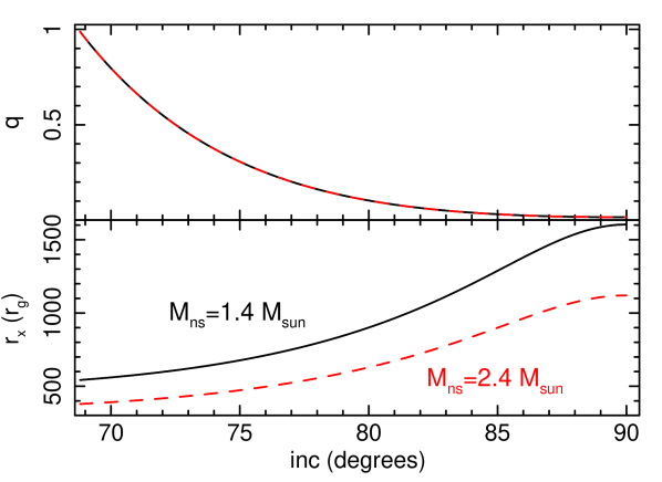
Figure 10: Radius of the X-ray emitting region (bottom) and mass ratio (top) inferred from the ingress duration and totality duration assuming that the companion star is an optically thick sphere with no surrounding material. Black solid and red dashed lines correspond to an assumed NS mass of $1.4~{}M_{\odot}$ and $2.4~{}M_{\odot}$ respectively.

Therefore, for a given inclination angle, we can calculate $r_{x}/r_{a}$ and $R_{\rm cs}/r_{a}$. We can then assume that the companion fills its Roche-Lobe in order to calculate the mass ratio $q$ from $R_{\rm cs}/r_{a}$ (Equation 8). In order to calculate $r_{x}$ as a function of $i$, we then only need to assume a NS mass and calculate $r_{a}$ from Kepler’s law.

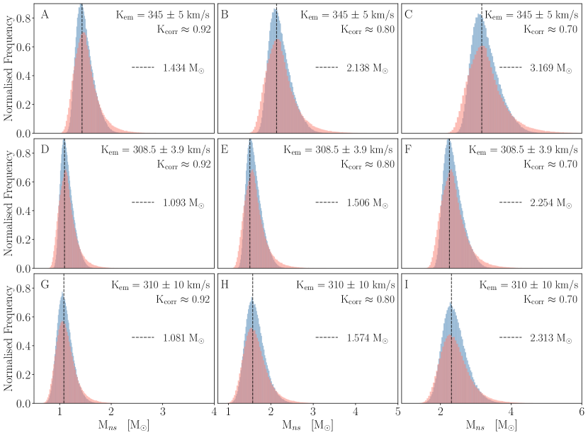
Figure 11: Panels A-I: Distributions of $M_{\rm{ns}}$ assuming the Gaussian (blue) and exponential (red) density profiles within the eclipse profile model calculated using a different combination of $K_{\rm em}$ and K-Correction, which are detailed in each panel. Also shown is a black dashed line corresponding to the mean peak NS mass. The K-correction in A, D and G corresponds to the most conservative value calculated using the mass ratio dependent relation of Munoz-Darias et al. (2005) (Equation 18) for our best fitting value $q=0.222$. Column 2 (B, E and H) and column 3 (C, F and I) assume the reasonable K-corrections of 0.8 and 0.7 respectively. Emission lines considered are 345 $\pm$ 5 km/s from He_II (Bassa et al., 2009), 310 $\pm$ 10 km/s from He_II (Muñoz-Darias et al., 2009) and 308.5 $\pm$ 3.9 km/s from a weighted average of H_β and H_γ (Ratti et al., 2012).

Figure 10 shows the resulting inferred values of $r_{x}$ and $q$ as a function of inclination angle for two values of NS mass. We see that $r_{x}$ increases with $i$, and recover the simple equation $r_{x}(i=90^{\circ})=\Delta\phi_{\rm in}r_{a}/2$ from the main text. For inclination lower than $\sim 69^{\circ}$, there is no solution for $q$. The smallest possible X-ray region under our assumptions is therefore $r_{x}\sim 400~{}r_{g}$. This is implausibly large, and adds to the argument that the ingress duration must instead be dominated by an extended stellar atmosphere and/or a layer or ablated material.

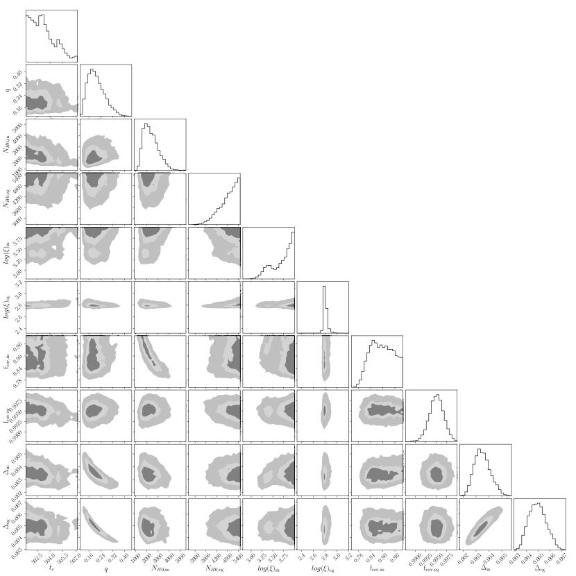
Figure 12: Output distributions from the MCMC simulation of the eclipse profile model with the Gaussian density profile with a chain length of 307200, a burn-in period of 92160 and 256 walkers. Hard upper limits of 5500 are used for the surface column densities, $N_{H0,\rm{in}}$ and $N_{H0,\rm{eg}}$ to prevent the walkers entering non-physical parts of parameters space. For the same reason the ionisation parameters, $\log(\xi)_{\rm{in}}$ and $\log(\xi)_{\rm{eg}}$, had an upper limit of 4.0. The lines and shading, dark to light, on the 2D histograms represent $1\sigma$, $2\sigma$ and $3\sigma$ contours respectively. The y-axes for the 1D histograms are in arbitrary units.

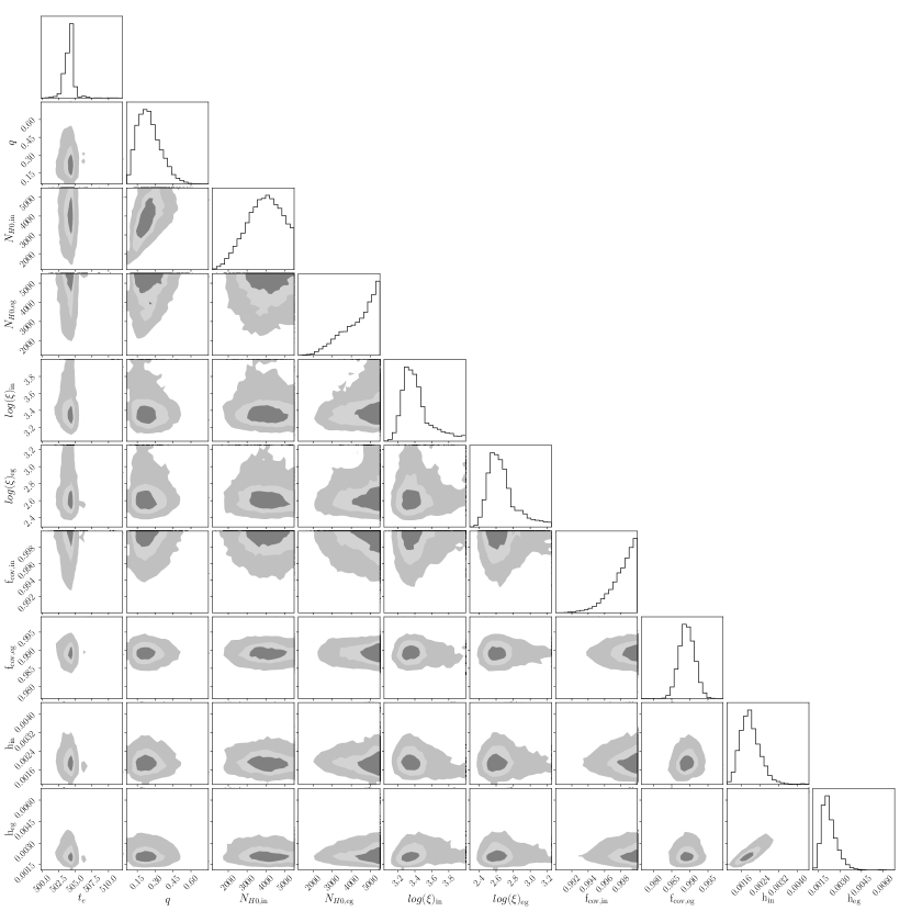
Figure 13: Output distributions from the MCMC simulation of the eclipse profile model with the exponential density profile with a chain length of 307200, a burn-in period of 92160 and 256 walkers. Hard upper limits of 5500 are used for the surface column densities, $N_{H0,\rm{in}}$ and $N_{H0,\rm{eg}}$ to prevent the walkers entering non-physical parts of parameters space. For the same reason the ionisation parameters, $\log(\xi)_{\rm{in}}$ and $\log(\xi)_{\rm{eg}}$, had an upper limit of 4.0. The lines and shading, dark to light, on the 2D histograms represent $1\sigma$, $2\sigma$ and $3\sigma$ contours respectively. The y-axes for the 1D histograms are in arbitrary units.

Appendix B Neutron Star Mass

Figure 11 is provided to show the posterior NS mass distributions obtained using $K_{\rm{em}}$ values from Bassa et al. 2009, Ratti et al. 2012 and Muñoz-Darias et al. 2009. Panels A, B and C assume $K_{\rm{em}}=345\pm 5$ km/s (Bassa et al., 2009). This value is subject to the same uncertainties as $K_{\rm{em}}=410\pm 5$ km/s (Bassa et al., 2009), which is presented in the main text and therefore, is not included in our primary analysis. Panels D, E and F assume $K_{\rm{em}}=308.5\pm 3.9$ km/s (Ratti et al., 2012). Panels G, H and I assume $K_{\rm{em}}=310\pm 10$ km/s (Muñoz-Darias et al., 2009). The latter two radial velocity measurements were not considered in the main text as they are lower than other measured radial velocities, indicating that they originated from a spatial zone further from the centre of mass of the companion and are, therefore, less constraining.

Appendix C Markov Chain Monte Carlo

To further understand the parameter space of the eclipse mapping model, we run a Markov Chain Monte Carlo (MCMC) simulation within xspec using the Goodman-Weare algorithm. We run 4 chains using the intrinsic routine chain, two assuming the Gaussian density profile and two assuming the exponential density profile. Each chain is run individually, ensuring that the chains assuming the same radial density profile are not correlated. We use a chain length of 307200 with a burn-in period of 92160. Each chain uses 256 walkers and starts, respectively, from their best fits presented in Table 4.

Our model assumes a constant out-of-eclipse spectrum so only parameters governing the eclipse profiles are variable during the fits. Therefore, we have 12 free parameters. Two of the parameters are simply normalise of the eclipse profiles such that the out-of-eclipse count rate equals 1.0 and the time at the centre of totality equals 0.0, so there are 10 key parameters we explore here: $t_{e}$, $q$, $N_{H0,\rm{in}}$, $N_{H0,\rm{eg}}$, $\log(\xi)_{\rm{in}}$, $\log(\xi)_{\rm{eg}}$ $\rm{f_{cov,in}}$, $\rm{f_{cov,in}}$, $\Delta_{\rm{in}}$, $\Delta_{\rm{eg}}$ (for the Gaussian density profile only), $\rm{h_{in}}$ and $\rm{h_{eg}}$ (exponential density profile only). Figures 12 and 13 show the output distributions for the Gaussian and exponential models respectively.

For the eclipse profile model with a Gaussian radial density profile, we see evidence of a positive correlation between $\Delta_{\rm{in}}$ and$\Delta_{\rm{eg}}$. Assuming a spherically symmetric system, it can be expected that the amount of material accumulating around the star to increase similarly on both sides. The mass ratio is anti-correlated with both $\Delta_{\rm{in}}$ and$\Delta_{\rm{eg}}$ which is expected from our formalism presented in Sections 3 and 4. Similarly, the scale heights, $\rm{h_{in}}$ and $\rm{h_{eg}}$ in the eclipse profile model with an exponential radial density profile display a slightly positive correlation. Similar physical arguments to those presented above can explain this relationship. No other correlations are present for these models.

The convergence of each chain is tested using the Geweke convergence measure which compares the mean of each parameter in two intervals of the chain, one shortly after the burn-in period and one towards the end of the chain. These correspond to the first $10\%$ and the last $50\%$ of the chain. For all chains, all parameters measured between $\pm 0.2$, indicating that convergence has been achieved. One parameter remains an exception to this: $N_{H0,\rm{eg}}$ in the eclipse profile model assuming an exponential density profile. This parameter measures as 0.545 and 0.551 for the two chains. The higher Geweke values here are likely a result of an upper limit on the parameter of 5500, which is in place to prevent the walkers from venturing into nonphysical parts of parameter space. Therefore, we remain confident in the convergence of the chain despite this result.

To increase our confidence in the convergence of the chains, we use the Rubin-Gelman convergence test to compare the variances of each parameter in the chain between two chains of the same length. For this test, we implement a stringent bound of $R_{c}<1.1$ as an indication of convergence, with higher values indicating parameters are varying too much and have not yet converged. For both models, all parameters give $R_{c}<1.05$, therefore we are confident in the convergence of the chains.

References

- Abbott et al. (2020a) Abbott B. P., et al., 2020a, The Astrophysical Journal, 892, L3
- Abbott et al. (2020b) Abbott R., et al., 2020b, The Astrophysical Journal, 896, L44
- Alpar et al. (1982) Alpar M. A., Chengt A. F., Ruderman M. A., Shaham J., 1982, Letters to Nature, 300, 728
- An et al. (2018) An H., Romani R. W., Kerr M., 2018, The Astrophysical Journal, 868, L8
- Antoniadis et al. (2016) Antoniadis J., Tauris T. M., Ozel F., Barr E., Champion D. J., Freire P. C. C., 2016
- Archibald et al. (2009) Archibald A. M., et al., 2009, Science, 324, 1411
- Arnaud et al. (1996) Arnaud K., Dorman B., Gordon C., 1996, 101, 17
- Bassa et al. (2009) Bassa C. G., Jonker P. G., Steeghs D., Torres M. A., 2009, Monthly Notices of the Royal Astronomical Society, 399, 2055
- Casares et al. (2014) Casares J., Negueruela I., Ribó M., Ribas I., Paredes J. M., Herrero A., Simón-Díaz S., 2014, Nature, 505, 378
- Chakrabarty & Morgan (1998) Chakrabarty D., Morgan E. H., 1998, Nature Astronomy, 394, 346
- Chen & Chatziioannou (2020) Chen H.-Y., Chatziioannou K., 2020, The Astrophysical Journal, 893, L41
- Coleman Miller (2013) Coleman Miller M., 2013, Born Symposium Proceedings, 10, 1
- Coleman Miller et al. (2021) Coleman Miller M., et al., 2021, The Astrophysical Journal Letters, 918, L28
- Collier Cameron (1991) Collier Cameron A., 1991, Mem. Soc. Ast. It., 62, 338
- Collier Cameron (1996) Collier Cameron A., 1996, International Astronomical Union, 176, 449
- Cromartie et al. (2019) Cromartie H. T., et al., 2019, Nature Astronomy, 4, 72
- Damen et al. (1990) Damen E., Magnier E., Lewin W. H., Tan J., Penninx W., Van Paradijs J., 1990, Astronomy & Astrophysics, 237, 103
- De Marco & Ponti (2016) De Marco B., Ponti G., 2016, The Astrophysical Journal, 826, 70
- Degenaar et al. (2011) Degenaar N., et al., 2011, Monthly Notices of the Royal Astronomical Society, 412, 1409
- Done (2010) Done C., 2010, Accretion Processes In Astrophysics: IAC Winter School Of Astrophysics, 9781107030, 184
- Essick & Landry (2020) Essick R., Landry P., 2020, The Astrophysical Journal, 904, 80
- Fattoyev et al. (2020) Fattoyev F. J., Horowitz C. J., Piekarewicz J., Reed B., 2020, Physical Review C, 102, 1
- Ferreira (2000) Ferreira J. M., 2000, Monthly Notices of the Royal Astronomical Society, 316, 647
- Fonseca et al. (2021) Fonseca E., et al., 2021, The Astrophysical Journal Letters, 915, L12
- Fruchter et al. (1988) Fruchter A. S., Stinebring D. R., Taylor J. H., 1988, Nature, 333, 237
- Fruchter et al. (1990) Fruchter A. S., et al., 1990, The Astrophysical Journal, 351, 642
- Fujimoto & Taam (1986) Fujimoto M. Y., Taam R. E., 1986, The Astrophysical Journal, 305, 246
- Galloway et al. (2010) Galloway D. K., Lin J., Chakrabarty D., Hartman J. M., 2010, Astrophysical Journal Letters, 711, 148
- Güver et al. (2010) Güver T., Wroblewski P., Camarota L., Özel F., 2010, Astrophysical Journal, 719, 1807
- Horne (1985) Horne K., 1985, Monthly Notices of the Royal Astronomical Society, 213, 2043
- Jiménez-Ibarra et al. (2018) Jiménez-Ibarra F., Muñoz-Darias T., Wang L., Casares J., Sánchez D. M., Steeghs D., Padilla M. A., Charles P. A., 2018, Monthly Notices of the Royal Astronomical Society, 474, 4717
- Johns-Krull & Valenti (1996) Johns-Krull C. M., Valenti J. A., 1996, The Astrophysical Journal, 459, 1
- Kaltenegger & Traub (2008) Kaltenegger L., Traub W. A., 2008, Astrophysical Journal, 698, 519
- Kochukhov (2021) Kochukhov O., 2021, Magnetic fields of M dwarfs. Vol. 29, Springer Berlin Heidelberg (arXiv:2011.01781), doi:10.1007/s00159-020-00130-3, https://doi.org/10.1007/s00159-020-00130-3
- Lecavelier Des Etangs et al. (2010) Lecavelier Des Etangs A., et al., 2010, Astronomy and Astrophysics, 514, 1
- Lewin et al. (1993) Lewin W. H., Van Paradijs J., Taam R. E., 1993, Space Science Reviews, 62, 223
- Linares (2014) Linares M., 2014, Astrophysical Journal, 795, 72
- Lindblom (1992) Lindblom L., 1992, The Astrophysical Journal, 398, 569
- Marsh et al. (1994) Marsh T. R., Robinson E. L., Wood J. H., 1994, Monthly Notices of the Royal Astronomical Society, 266, 137
- Mikles & Hynes (2012) Mikles V. J., Hynes R. I., 2012, Astrophysical Journal, 750, 1
- Miller et al. (2006) Miller L., Turner T. J., Reeves J. N., George I. M., Porquet D., Nandra K., Dovciak M., 2006, Astronomy and Astrophysics, 453, 7
- Miraval Zanon et al. (2021) Miraval Zanon A., et al., 2021, Astronomy & Astrophysics, 649, A120
- Moore & Horwitz (2007) Moore T. E., Horwitz J. L., 2007, Reviews of Geophysics, 45, 1
- Muñoz-Darias et al. (2009) Muñoz-Darias T., Casares J., O’Brien K., Steeghs D., Martínez-Pais I. G., Cornelisse R., Charles P. A., 2009, Monthly Notices of the Royal Astronomical Society: Letters, 394, 136
- Munoz-Darias et al. (2005) Munoz-Darias T., Casares J., Martinez-Pais I. G., 2005, The Astrophysical Journal, 635, 502
- Özel (2006) Özel F., 2006, Nature, 441, 1115
- Özel & Freire (2016) Özel F., Freire P., 2016, Annual Review of Astronomy and Astrophysics, 54, 401
- Papitto et al. (2013) Papitto A., et al., 2013, Nature, 501, 517
- Parikh et al. (2021) Parikh A. S., Degenaar N., Hernández Santisteban J. V., Wijnands R., Psaradaki I., Costantini E., Modiano D., Miller J. M., 2021, Monthly Notices of the Royal Astronomical Society, 501, 1453
- Parmar et al. (1986) Parmar A. N., White N. E., Giommo P., Gottwald M., 1986, The Astrophysical Journal, 308
- Parmar et al. (1991) Parmar A. N., Smale A., Verbunt F., Corbet R. H. D., 1991, The Astrophysical Journal, 366, 253
- Pearson et al. (2006) Pearson K. J., et al., 2006, The Astrophysical Journal, 648, 1169
- Podsiadlowski (2009) Podsiadlowski P., 2009, Evolution of Binary Systems. https://doi.org/10.1017/CBO9781139343268.003
- Pols (2011) Pols O., 2011, Stellar Structure and Evolution. No. September
- Pols et al. (1998) Pols O. R., Schröder K. P., Hurley J. R., Tout C. A., Eggleton P. P., 1998, Monthly Notices of the Royal Astronomical Society, 298, 525
- Polzin et al. (2018) Polzin E. J., et al., 2018, Monthly Notices of the Royal Astronomical Society, 476, 1968
- Polzin et al. (2020) Polzin E. J., Breton R. P., Bhattacharyya B., Scholte D., Sobey C., Stappers B. W., 2020, Monthly Notices of the Royal Astronomical Society, 494, 2948
- Ponti et al. (2014) Ponti G., Muñoz-Darias T., Fender R. P., 2014, Monthly Notices of the Royal Astronomical Society, 444, 1829
- Postnov & Yungelson (2014) Postnov K. A., Yungelson L. R., 2014, Living Reviews in Relativity, 9, 6
- Poutanen & Gierliński (2003) Poutanen J., Gierliński M., 2003, Monthly Notices of the Royal Astronomical Society, 343, 1301
- Providência (2019) Providência C., 2019, AIP Conference Proceedings, 2127, 20022
- Puls et al. (2008) Puls J., Vink J. S., Najarro F., 2008, Astronomy and Astrophysics Review, 16, 209
- Radhakrishnan & Srinivasan (1982) Radhakrishnan V., Srinivasan G., 1982, Current Science, 51, 1096
- Raithel et al. (2018) Raithel C. A., Sukhbold T., Özel F., 2018, The Astrophysical Journal, 856, 35
- Rapisarda et al. (2016) Rapisarda S., Ingram A., Kalamkar M., van der Klis M., 2016, Monthly Notices of the Royal Astronomical Society, 462, 4078
- Ratti et al. (2012) Ratti E. M., Steeghs D. T. H., Jonker P. G., Torres M. A. P., Bassa C. G., Verbunt F., 2012, Monthly Notices of the Royal Astronomical Society, 420, 75
- Riley et al. (2019) Riley T. E., et al., 2019, The Astrophysical Journal, 887, L21
- Shulyak et al. (2019) Shulyak D., et al., 2019, Astronomy and Astrophysics, 626, 1
- Somero et al. (2012) Somero A., Hakala P., Muhli P., Charles P., Vilhu O., 2012, A&A, 539, A111
- Steeghs et al. (1996) Steeghs D., Horne K., Marsh T. R., Donati J. F., 1996, Monthly Notices of the Royal Astronomical Society, 281, 626
- Steiner et al. (2010) Steiner A. W., Lattimer J. M., Brown E. F., 2010, Astrophysical Journal, 722, 33
- Sukhbold et al. (2018) Sukhbold T., Woosley S. E., Heger A., 2018, The Astrophysical Journal, 860, 93
- Sztajno et al. (1987) Sztajno M., Fujimoto M. Y., Van Paradijs J., Vacca W. D., Lewin W. H., Penninx W., Trumper J., 1987, Monthly Notices of the Royal Astronomical Society, 226, 39
- Tendulkar et al. (2014) Tendulkar S., et al., 2014, Astrophysical Journal, 791, 77
- Van Paradijs (1979) Van Paradijs J., 1979, The Astrophysical Journal, 91, 498
- Vanderburg et al. (2015) Vanderburg A., et al., 2015, Nature, 526, 546
- Voisin et al. (2020) Voisin G., Cognard I., Freire P. C. C., Wex N., Guillemot L., Desvignes G., Kramer M., Theureau G., 2020, Astronomy & Astrophysics, 638, A24
- Wade & Horne (1988) Wade R. A., Horne K., 1988, The Astrophysical Journal, 324, 411
- Wang et al. (2017) Wang L., Steeghs D., Casares J., Charles P. A., Muñoz-Darias T., Marsh T. R., Hynes R. I., O’Brien K., 2017, Monthly Notices of the Royal Astronomical Society, 466, 2261
- Wargelin & Drake (2002) Wargelin B. J., Drake J. J., 2002, The Astrophysical Journal, 578, 503
- Wilms et al. (2000) Wilms J., Allen A., McCray R., 2000, The Astrophysical Journal, 542, 914
- Wolff et al. (2009) Wolff M. T., Ray P. S., Wood K. S., Hertz P. L., 2009, Astrophysical Journal, Supplement Series, 183, 156
- Yang et al. (2018) Yang H., East W. E., Lehner L., 2018, The Astrophysical Journal, 856, 110
- Zdziarski et al. (1996) Zdziarski A. A., Johnson W. N., Magdziarz P., 1996, Monthly Notices of the Royal Astronomical Society, 283, 193