Admissible Policy Teaching through Reward Design

Abstract

We study reward design strategies for incentivizing a reinforcement learning agent to adopt a policy from a set of admissible policies. The goal of the reward designer is to modify the underlying reward function cost-efficiently while ensuring that any approximately optimal deterministic policy under the new reward function is admissible and performs well under the original reward function. This problem can be viewed as a dual to the problem of optimal reward poisoning attacks: instead of forcing an agent to adopt a specific policy, the reward designer incentivizes an agent to avoid taking actions that are inadmissible in certain states. Perhaps surprisingly, and in contrast to the problem of optimal reward poisoning attacks, we first show that the reward design problem for admissible policy teaching is computationally challenging, and it is NP-hard to find an approximately optimal reward modification. We then proceed by formulating a surrogate problem whose optimal solution approximates the optimal solution to the reward design problem in our setting, but is more amenable to optimization techniques and analysis. For this surrogate problem, we present characterization results that provide bounds on the value of the optimal solution. Finally, we design a local search algorithm to solve the surrogate problem and showcase its utility using simulation-based experiments.

Introduction

Reinforcement learning (RL) (Sutton and Barto 2018) is a framework for deriving an agent’s policy that maximizes its utility in sequential decision making tasks. In the standard formulation, the utility of an agent is defined via its reward function, which determines the decision making task of interest. Reward design plays a critical role in providing sound specifications of the task goals and supporting the agent’s learning process (Singh, Lewis, and Barto 2009; Amodei et al. 2016).

There are different perspectives on reward design, which differ in the studied objectives. A notable example of reward design is reward shaping (Mataric 1994; Dorigo and Colombetti 1994; Ng, Harada, and Russell 1999) which modifies the reward function in order to accelerate the learning process of an agent. Reward transformations that are similar to or are based on reward shaping are not only used for accelerating learning. For example, reward penalties are often used in safe RL to penalize the agent whenever it violates safety constraints (Tessler, Mankowitz, and Mannor 2018). Similarly, reward penalties can be used in offline RL for ensuring robustness against model uncertainty (Yu et al. 2020), while exploration bonuses can be used as intrinsic motivation for an RL agent to reduce uncertainty (Bellemare et al. 2016).

In this paper, we consider a different perspective on reward design, and study it in the context of policy teaching and closely related (targeted) reward poisoning attacks. In this line of work (Zhang and Parkes 2008; Zhang, Parkes, and Chen 2009; Ma et al. 2019; Rakhsha et al. 2020b, a), the reward designer perturbs the original reward function to influence the choice of policy adopted by an optimal agent. For instance, (Zhang and Parkes 2008; Zhang, Parkes, and Chen 2009) studied policy teaching from a principal’s perspective who provides incentives to an agent to influence its policy. In reward poisoning attacks (Ma et al. 2019; Rakhsha et al. 2020b, a), an attacker modifies the reward function with the goal of forcing a specific target policy of interest. Importantly, the reward modifications do not come for free, and the goal in this line of work is to alter the original reward function in a cost-efficient manner. The associated cost can, e.g., model the objective of minimizing additional incentives provided by the principal or ensuring the stealthiness of the attack.

The focus of this paper is on a dual problem to reward poisoning attacks. Instead of forcing a specific target policy, the reward designer’s goal is to incentivize an agent to avoid taking actions that are inadmissible in certain states, while ensuring that the agent performs well under the original reward function. As in reward poisoning attacks, the reward designer cares about the cost of modifying the original reward function. Interestingly and perhaps surprisingly, the novel reward design problem leads to a considerably different characterization results, as we show in this paper. We call this problem admissible policy teaching since the reward designer aims to maximize the agent’s utility w.r.t. the original reward function, but under constraints on admissibility of state-action pairs. These constraints could encode additional knowledge that the reward designer has about the safety and security of executing certain actions. Our key contributions are:

• We develop a novel optimization framework based on Markov Decision Processes (MDPs) for finding a minimal reward modifications which ensure that an optimal agent adopts a well-performing admissible policy.

• We show that finding an optimal solution to the reward design problem for admissible policy teaching is computationally challenging, in particular, that it is NP-hard to find a solution that approximates the optimal solution.

• We provide characterization results for a surrogate problem whose optimal solution approximates the optimal solution to our reward design problem. For a specific class of MDPs, which we call special MDPs, we present an exact characterization of the optimal solution. For general MDPs, we provide bounds on the optimal solution value.

• We design a local search algorithm for solving the surrogate problem, and demonstrate its efficacy using simulation-based experiments.

Related Work

Reward design.

A considerable number of works is related to designing reward functions that improve an agent’s learning procedures. The optimal reward problem focuses on finding a reward function that can support computationally bounded agents (Sorg, Singh, and Lewis 2010; Sorg, Lewis, and Singh 2010). Reward shaping (Mataric 1994; Dorigo and Colombetti 1994), and in particular, potential-based reward shaping (Ng, Harada, and Russell 1999) and its extensions (e.g., (Devlin and Kudenko 2012; Grześ 2017; Zou et al. 2019)) densify the reward function so that the agent receives more immediate signals about its performance, and hence learns faster. As already mentioned, similar reward transformations, such as reward penalties or bonuses, are often used for reducing uncertainty or for ensuring safety constraints (Bellemare et al. 2016; Yu et al. 2020; Tessler, Mankowitz, and Mannor 2018). Related to safe and secure RL are works that study reward specification problem and negative side affects of reward misspecification (Amodei et al. 2016; Hadfield-Menell et al. 2017). The key difference between the above papers and our work is that we focus on policy teaching rather than on an agent’s learning procedures.

Teaching and steering.

As already explained, our work relates to prior work on policy teaching and targeted reward poisoning attacks (Zhang and Parkes 2008; Zhang, Parkes, and Chen 2009; Ma et al. 2019; Huang and Zhu 2019; Rakhsha et al. 2020b, a; Zhang et al. 2020b; Sun, Huo, and Huang 2021). Another line of related work is on designing steering strategies. For example, (Nikolaidis et al. 2017; Dimitrakakis et al. 2017; Radanovic et al. 2019) consider two-agent collaborative settings where a dominant agent can exert influence on the other agent, and the goal is to design a policy for the dominant agent that accounts for the imperfections of the other agent. Similar support mechanisms based on providing advice or helpful interventions have been studied by (Amir et al. 2016; Omidshafiei et al. 2019; Tylkin, Radanovic, and Parkes 2021). In contrast, we consider steering strategies based on reward design. When viewed as a framework for supporting an agent’s decision making, this paper is also related to works on designing agents that are robust against adversaries (Pinto et al. 2017; Fischer et al. 2019; Lykouris et al. 2019; Zhang et al. 2020a, 2021a, 2021b; Banihashem, Singla, and Radanovic 2021). These works focus on agent design and are complementary to our work on reward design.

Problem Setup

In this section we formally describe our problem setup.

Environment

The environment in our setting is described by a discrete-time Markov Decision Process (MDP) $M=(S,A,R,P,\gamma,\sigma)$, where $S$ and $A$ are the discrete finite state and action spaces respectively, $R:S\times A\rightarrow\mathds{R}$ is a reward function, $P:S\times A\times S\rightarrow[0,1]$ specifies the transition dynamics with $P(s,a,s^{\prime})$ denoting the probability of transitioning to state $s^{\prime}$ from state $s$ by taking action $a$, $\gamma\in[0,1)$ is the discounted factor, and $\sigma$ is the initial state distribution. A deterministic policy $\pi$ is a mapping from states to actions, i.e., $\pi:S\rightarrow A$, and the set of all deterministic policies is denoted by $\Pi_{\text{det}}$.

Next, we define standard quantities in this MDP, which will be important for our analysis. First, we define the score of a policy $\pi$ as the total expected return scaled by $1-\gamma$, i.e., ${\rho}^{\pi,R}=\mathbb{E}\left[(1-\gamma)\sum_{t=1}^{\infty}\gamma^{t-1}R(s_{t},a_{t})|\pi,\sigma\right]$. Here states $s_{t}$ and actions $a_{t}$ are obtained by executing policy $\pi$ starting from state $s_{1}$, which is sampled from the initial state distribution $\sigma$. Score ${\rho}^{\pi,R}$ can be obtained through state occupancy measure ${\mu}^{\pi}$ by using the equation ${\rho}^{\pi,R}=\sum_{s}{\mu}^{\pi}(s)\cdot R(s,\pi(s))$. Here, ${\mu}^{\pi}$ is the expected discounted state visitation frequency when $\pi$ is executed, given by ${\mu}^{\pi}(s)=\mathbb{E}\left[(1-\gamma)\sum_{t=1}^{\infty}\gamma^{t-1}\mathds{1}\left[s_{t}=s\right]|\pi,\sigma\right]$. Note that ${\mu}^{\pi}(s)$ can be equal to $0$ for some states. Furthermore, we define ${\mu}^{\pi}_{\textnormal{min}}=\min_{s|{\mu}^{\pi}(s)>0}{\mu}^{\pi}(s)$—the minimum always exists due to the finite state and action spaces. Similarly, we denote by ${\mu}_{\textnormal{min}}$ the minimal value of ${\mu}^{\pi}_{\textnormal{min}}$ across all deterministic policies, i.e., ${\mu}_{\textnormal{min}}=\min_{\pi\in\Pi_{\text{det}}}{\mu}^{\pi}_{\textnormal{min}}$.

We define the state-action value function, or $Q$ values as $Q^{\pi,R}(s,a)=\mathbb{E}\left[\sum_{t=1}^{\infty}\gamma^{t-1}R(s_{t},a_{t})|\pi,s_{1}=s,a_{1}=a\right]$, where states $s_{t}$ and actions $a_{t}$ are obtained by executing policy $\pi$ starting from state $s_{1}=s$ in which action $a_{1}=a$ is taken. State-action values $Q(s,a)$ relate to score $\rho$ via the equation ${\rho}^{\pi,R}=\mathbb{E}_{s\sim\sigma}\left[(1-\gamma)\cdot Q^{\pi,R}(s,\pi(s))\right]$, where the expectation is taken over possible starting states.

Agent and Reward Functions

We consider a reinforcement learning agent whose behavior is specified by a deterministic policy $\pi$, derived offline using an MDP model given to the agent. We assume that the agent selects a deterministic policy that (approximately) maximizes the agent’s expected utility under the MDP model specified by a reward designer. In other words, given an access to the MDP $M=(S,A,R,P,\gamma,\sigma)$, the agent chooses a policy from the set $\textsc{{Opt}}^{\epsilon}_{\textnormal{det}}(R)=\{\pi\in\Pi_{\text{det}}:{\rho}^{\pi,R}>\max_{\pi^{\prime}\in\Pi_{\text{det}}}{\rho}^{\pi^{\prime},R}-\epsilon\}$, where $\epsilon$ is a strictly positive number. It is important to note that the MDP model given to the agent might be different from the true MDP model of the environment. In this paper, we focus on the case when only the reward functions of these two MDPs (possibly) differ.

Therefore, in our notation, we differentiate the reward function that the reward designer specifies to the agent, denoting it by $\widehat{R}$, from the original reward function of the environment, denoting it by $\overline{R}$. A generic reward function is denoted by $R$, and is often used as a variable in our optimization problems. We also denote by $\pi^{*}$ a deterministic policy that is optimal with respect to $\overline{R}$ for any starting state, i.e., $Q^{\pi^{*},\overline{R}}(s,\pi^{*}(s))=\max_{\pi\in\Pi_{\text{det}}}Q^{\pi,\overline{R}}(s,\pi(s))$ for all states $s$.

Reward Designer and Problem Formulation

We take the perspective of a reward designer whose goal is to design a reward function, $\widehat{R}$, such that the agent adopts a policy from a class of admissible deterministic policies $\Pi^{\textnormal{adm}}_{\textnormal{det}}\subseteq\Pi_{\text{det}}$. Ideally, the new reward function $\widehat{R}$ would be close to the original reward function $\overline{R}$, thus reducing the cost of the reward design. At the same time, the adopted policy should perform well under the original reward function $\overline{R}$, since this is the performance that the reward designer wants to optimize and represents the objective of the underlying task. As considered in related works (Ma et al. 2019; Rakhsha et al. 2020b, a), we measure the cost of the reward design by $L_{2}$ distance between the designed $\widehat{R}$ and the original reward function $\overline{R}$. Moreover, we measure the agent’s performance with the score ${\rho}^{\pi,\overline{R}}$, where the agent’s policy $\pi$ is obtained w.r.t. the designed reward function $\widehat{R}$. Given the model of the agent discussed in the previous subsection, and assuming the worst-case scenario (w.r.t. the tie-breaking in the policy selection), the following optimization problem specifies the reward design problem for admissible policy teaching (APT):

$$\quad\min_{R}\max_{\pi}\left\lVert\overline{R}-R\right\rVert_{2}-\lambda\cdot{\rho}^{\pi,\overline{R}}$$

$$\quad\mbox{ s.t. }\quad\textsc{{Opt}}^{\epsilon}_{\textnormal{det}}(R)\subseteq\Pi^{\textnormal{adm}}_{\textnormal{det}}$$

$$\quad\quad\quad\quad\pi\in\textsc{{Opt}}^{\epsilon}_{\textnormal{det}}(R),$$

where $\lambda\geq 0$ is a trade-off factor. While in this problem formulation $\Pi^{\textnormal{adm}}_{\textnormal{det}}$ can be any set of policies, we will primarily focus on admissible policies that can be described by a set of admissible actions per state. More concretely, we define sets of admissible actions per state denoted by $A^{\textnormal{adm}}_{s}\subseteq A$. Given these sets $A^{\textnormal{adm}}_{s}$, the set of admissible policies will be identified as $\Pi^{\textnormal{adm}}_{\textnormal{det}}=\{\pi|\pi(s)\in A^{\textnormal{adm}}_{s}\lor{\mu}^{\pi}(s)=0\mbox{ for }s\in S\}$. In other words, these policies must take admissible actions for states that have non-zero state occupancy measure.

We conclude this section by validating the soundness of the optimization problem (Reward Designer and Problem Formulation). The following proposition shows that the optimal solution to the optimization problem (Reward Designer and Problem Formulation) is always attainable.

Proposition 1.

If $\Pi^{\textnormal{adm}}_{\textnormal{det}}$ is not empty, there always exists an optimal solution to the optimization problem (Reward Designer and Problem Formulation).

In the following sections, we analyze computational aspects of this optimization problem, showing that it is intractable in general and providing characterization results that bound the value of solutions. The proofs of our results are provided in the full version of the paper.

Computational Challenges

We start by analyzing computational challenges behind the optimization problem (Reward Designer and Problem Formulation). To provide some intuition, let us first analyze a special case of (Reward Designer and Problem Formulation) where $\lambda=0$, which reduces to the following optimization problem:

$$\quad\min_{R}\left\lVert\overline{R}-R\right\rVert_{2}$$

$$\quad\mbox{ s.t. }\quad\textsc{{Opt}}^{\epsilon}_{\textnormal{det}}(R)\subseteq\Pi^{\textnormal{adm}}_{\textnormal{det}}.$$

This special case of the optimization problem with $\lambda=0$ is a generalization of the reward poisoning attack from (Rakhsha et al. 2020b, a). In fact, the reward poisoning attack of (Rakhsha et al. 2020a) can be written as

$$\quad\min_{R}\left\lVert\overline{R}-R\right\rVert_{2}$$

$$\quad\mbox{ s.t. }\quad\textsc{{Opt}}^{\epsilon}_{\textnormal{det}}(R)\subseteq\{\pi|\pi(s)={\pi_{\dagger}}(s)\mbox{ if }\mu^{{\pi_{\dagger}}}(s)>0\},$$

where ${\pi_{\dagger}}$ is the target policy that the attacker wants to force. However, while (Computational Challenges) is tractable in the setting of (Rakhsha et al. 2020a), the same is not true for (Computational Challenges); see Remark 1. Intuitively, the difficulty of solving the optimization problem (Computational Challenges) lies in the fact that the policy set $\Pi^{\textnormal{adm}}_{\textnormal{det}}$ (in the constraints of (Computational Challenges)) can contain exponentially many policies. Since the optimization problem (Computational Challenges) is a specific instance of the optimization problem (Reward Designer and Problem Formulation), the latter problem is also computationally intractable. We formalize this result in the following theorem.

Theorem 1.

For any constant $p\in(0,1)$, it is NP-hard to distinguish between instances of (Computational Challenges) that have optimal values at most $\xi$ and instances that have optimal values larger than $\xi\cdot\sqrt{(|S|\cdot|A|)^{1-p}}$. The result holds even when the parameters $\epsilon$ and $\gamma$ in (Computational Challenges) are fixed to arbitrary values subject to $\epsilon>0$ and $\gamma\in(0,1)$.

The proof of the theorem is based on a classical NP-complete problem called Exact-3-Set-Cover (X3C) (Karp 1972; Garey and Johnson 1979). The result implies that it is unlikely (assuming that P = NP is unlikely) that there exists a polynomial-time algorithm that always outputs an approximate solution whose cost is at most $\sqrt{(|S|\cdot|A|)^{1-p}}$ times that of the optimal solution for some $p>0$.

We proceed by introducing a surrogate problem (Computational Challenges), which is more amenable to optimization techniques and analysis since the focus is put on optimizing over policies rather than reward functions. In particular, the optimization problem takes the following form:

$$\quad\min_{\pi\in\Pi^{\textnormal{adm}}_{\textnormal{det}},R}\left\lVert\overline{R}-R\right\rVert_{2}-\lambda\cdot{\rho}^{\pi,\overline{R}}$$

$$\quad\quad\mbox{ s.t. }\quad\quad\textsc{{Opt}}^{\epsilon}_{\textnormal{det}}(R)\subseteq\{\pi^{\prime}|\pi^{\prime}(s)=\pi(s)\mbox{ if }\mu^{\pi}(s)>0\}.$$

Note that (Computational Challenges) differs from (Computational Challenges) in that it optimizes over all admissible policies, and it includes performance considerations in its objective. The result in Theorem 1 extends to this case as well, so the main computational challenge remains the same.

The following proposition shows that the solution to the surrogate problem (Computational Challenges) is an approximate solution to the optimization problem (Reward Designer and Problem Formulation), with an additive bound. More precisely:

Proposition 2.

Let $\widehat{R}_{1}$ and $\widehat{R}_{2}$ be the optimal solutions to (Reward Designer and Problem Formulation) and (Computational Challenges) respectively and let $l(R)$ be a function that outputs the objective of the optimization problem (Reward Designer and Problem Formulation), i.e.,

$$l(R)=\max_{\pi\in\textsc{{Opt}}^{\epsilon}_{\textnormal{det}}(R)}\left\lVert\overline{R}-R\right\rVert_{2}-\lambda{\rho}^{\pi,\overline{R}}.$$ (1)

Then $\widehat{R}_{2}$ satisfies the constraints of (Reward Designer and Problem Formulation), i.e, $\textsc{{Opt}}^{\epsilon}_{\textnormal{det}}(\widehat{R}_{2})\subseteq\Pi^{\textnormal{adm}}_{\textnormal{det}}$, and

$$l(\widehat{R}_{1})\leq l(\widehat{R}_{2})\leq l(\widehat{R}_{1})+\frac{\epsilon}{{\mu}_{\min}}\cdot\sqrt{|S|\cdot|A|}.$$

Due to this result, in the following sections, we focus on the optimization problem (Computational Challenges), and provide characterization for it. Using Proposition 2 we can obtain analogous results for the optimization problem (Reward Designer and Problem Formulation).

Remark 1.

The optimization problem (Computational Challenges) is a strictly more general version of the optimization problem studied in (Rakhsha et al. 2020a) since (Computational Challenges) does not require ${\mu}^{\pi}(s)>0$ for all $\pi$ and $s$. This fact also implies that the algorithmic approach presented in (Rakhsha et al. 2020a) is not applicable in our case. hm with provable guarantees. We provide an efficient algorithm for finding an approximate solution to (Computational Challenges) with provable guarantees in the full version of the paper.

Characterization Results for Special MDPs

In this section, we consider a family of MDPs where an agent’s actions do not influence transition dynamics, or more precisely, all the actions influence transition probabilities in the same way. In other words, the transition probabilities satisfy $P(s,a,s^{\prime})=P(s,a^{\prime},s^{\prime})$, for all $s$, $a$, $a^{\prime}$, $s^{\prime}$. We call this family of MDPs special MDPs, in contrast to general MDPs that are studied in the next section. Since an agent’s actions do not influence the future, the agent can reason myopically when deciding on its policy. Therefore, the reward designer can also treat each state separately when reasoning about the cost of the reward design. Importantly, the hardness result from the previous section does not apply for this instance of our setting, so we can efficiently solve the optimization problems (Reward Designer and Problem Formulation) and (Computational Challenges).

Forcing Myopic Policies

We first analyze the cost of forcing a target policy ${\pi_{\dagger}}$ in special MDPs. The following lemma plays a critical role in our analysis.

Lemma 1.

Consider a special MDP with reward function $\overline{R}$, and let $\pi^{*}_{\textnormal{adm}}(s)=\operatorname*{arg\,max}_{a\in\Pi^{\textnormal{adm}}_{\textnormal{det}}}\overline{R}(s,a)$. Then the cost of the optimal solution to the optimization problem (Computational Challenges) with ${\pi_{\dagger}}=\pi^{*}_{\textnormal{adm}}$ is less than or equal to the cost of the optimal solution to the optimization problem (Computational Challenges) with ${\pi_{\dagger}}=\pi$ for any $\pi\in\Pi^{\textnormal{adm}}_{\textnormal{det}}$.

In other words, Lemma 1 states that in special MDPs it is easier to force policies that are myopically optimal (i.e., optimize w.r.t. the immediate reward) than any other policy in the admissible set $\Pi^{\textnormal{adm}}_{\textnormal{det}}$. This property is important for the optimization problem (Computational Challenges) since its objective includes the cost of forcing an admissible policy.

Analysis of the Reward Design Problem

We now turn to the reward design problem (Computational Challenges) and provide characterization results for its optimal solution. Before stating the result, we note that for special MDPs ${\mu}^{\pi}(s)$ is independent of policy $\pi$, so we denote it by ${\mu}(s)$.

Theorem 2.

Consider a special MDP with reward function $\overline{R}$. Define $\widehat{R}(s,a)=\overline{R}(s,a)$ for ${\mu}(s)=0$ and otherwise

$$\widehat{R}(s,a)=\begin{cases}x_{s}+\frac{\epsilon}{{\mu}(s)}\quad&\mbox{ if }a=\pi^{*}_{\textnormal{adm}}(s)\\ x_{s}\quad&\mbox{ if }a\neq\pi^{*}_{\textnormal{adm}}(s)\land\overline{R}(s,a)\geq x_{s}\\ \overline{R}(s,a)\quad&\mbox{ otherwise}\end{cases},$$

where $x_{s}$ is the solution to the equation

$$\sum_{a\neq\pi^{*}_{\textnormal{adm}}(s)}\left[\overline{R}(s,a)-x\right]^{+}=x-\overline{R}(s,\pi^{*}_{\textnormal{adm}}(s))+\frac{\epsilon}{{\mu}(s)}.$$

Then, $(\pi^{*}_{\textnormal{adm}},\widehat{R})$ is an optimal solution to (Computational Challenges).

Theorem 2 provides an interpretable solution to (Computational Challenges): for each state-action pair $(s,a\neq\pi^{*}_{\textnormal{adm}}(s))$ we reduce the corresponding reward $\overline{R}(s,a)$ if it exceeds a state dependent threshold. Likewise, we increase the rewards $\overline{R}(s,\pi^{*}_{\textnormal{adm}}(s))$.

Characterization Results for General MDPs

In this section, we extend the characterization results from the previous section to general MDPs for which transition probabilities can depend on actions. In contrast to the previous section, the computational complexity result from Theorem 1 showcase the challenge of deriving characterization results for general MDPs that specify the form of an optimal solution. We instead focus on bounding the value of an optimal solution to (Computational Challenges) relative to the score of an optimal policy $\pi^{*}$. More specifically, we define the relative value $\Phi$ as

$$\Phi=\underbrace{\left\lVert\overline{R}-\widehat{R}_{2}\right\rVert_{2}}_{\text{cost}}+\lambda\cdot\underbrace{[{\rho}^{\pi^{*},\overline{R}}-{\rho}^{\pi_{2},\overline{R}}]}_{\text{performance reduction}},$$

where $(\pi_{2},\widehat{R}_{2})$ is an optimal solution to the optimization problem (Computational Challenges). Intuitively, $\Phi$ expresses the optimal value of (Computational Challenges) in terms of the cost of the reward design and the agent’s performance reduction.

The characterization results in this section provide bounds on $\Phi$ and are obtained by analyzing two specific policies: an optimal admissible policy $\pi^{*}_{\textnormal{adm}}\in\arg\max_{\pi\in\Pi^{\textnormal{adm}}_{\textnormal{det}}}{\rho}^{\pi,\overline{R}}$ that optimizes for performance ${\rho}$, and a min-cost policy $\pi_{\textnormal{min}_{c}}$ that minimizes the cost of the reward design and is a solution to the optimization problem (Computational Challenges) with $\lambda=0$. As we show in the next two subsections, bounding the cost of forcing $\pi^{*}_{\textnormal{adm}}$ and $\pi_{\textnormal{min}_{c}}$ can be used for deriving bounds on $\Phi$. Next, we utilize the insights of the characterization results to devise a local search algorithm for solving the reward design problem, whose utility we showcase using experiments.

Perspective 1: Optimal Admissible Policy

Let us consider an optimal admissible policy $\pi^{*}_{\textnormal{adm}}\in\arg\max_{\pi\in\Pi^{\textnormal{adm}}_{\textnormal{det}}}{\rho}^{\pi,\overline{R}}$. Following the approach presented in the previous section, we can design $\widehat{R}$ by (approximately) solving the optimization problem (Computational Challenges) (see Remark 1) with the target policy ${\pi_{\dagger}}=\pi^{*}_{\textnormal{adm}}$. While this approach does not yield an optimal solution for general MDPs, the cost of its solution can be bounded by a quantity that depends on the gap between the scores of an optimal policy $\pi^{*}$ and an optimal admissible policy $\pi^{*}_{\textnormal{adm}}$.

In particular, for any policy $\pi$ we can define the performance gap as ${\Delta_{{\rho}}^{\pi}}={\rho}^{\pi^{*},\overline{R}}-{\rho}^{\pi,\overline{R}}$. As we will show, the cost of forcing policy $\pi$ can be upper and lower bounded by terms that linearly depend on ${\Delta_{{\rho}}^{\pi}}$. Consequently, this means that one can also bound $\Phi$ with terms that linearly depend on ${\Delta_{{\rho}}}=\min_{\pi}{\Delta_{{\rho}}^{\pi}}$, which is nothing else but the performance gap of $\pi=\pi^{*}_{\textnormal{adm}}$. Formally, we obtain the following result.

Theorem 3.

The relative value $\Phi$ is bounded by

$$\alpha_{{\rho}}\cdot{\Delta_{{\rho}}}\leq\Phi\leq\beta_{{\rho}}\cdot{\Delta_{{\rho}}}+\frac{\epsilon}{{\mu}_{\min}}\cdot\sqrt{|S|\cdot|A|},$$

where $\alpha_{\rho}=\left(\lambda+\frac{1-\gamma}{2}\right)$ and $\beta_{{\rho}}=\left(\lambda+\frac{1}{{\mu}_{\min}}\right)$.

Note that the bounds in the theorem can be efficiently computed from the MDP parameters. Moreover, the reward design approach based on forcing $\pi^{*}_{\textnormal{adm}}$ yields a solution to (Computational Challenges) whose value (relative to the score of $\pi^{*}$) satisfies the bounds in Theorem 3. We use this approach as a baseline.

Perspective 2: Min-Cost Admissible Policy

We now take a different perspective, and compare $\Phi$ to the cost of the reward design obtained by forcing the min-cost policy $\pi_{\textnormal{min}_{c}}$. Ideally, we would relate $\Phi$ to the the smallest cost that the reward designer can achieve. However, this cost is not efficiently computable (due to Theorem 1), making such a bound uninformative.

Instead, we consider $Q$ values: as Ma et al. (2019) showed, the cost of forcing a policy can be upper and lower bounded by a quantity that depends on $Q$ values. We introduce a similar quantity, denoted by ${\Delta_{Q}}$ and defined as

$${\Delta_{Q}}=\min_{\pi\in\Pi^{\textnormal{adm}}_{\textnormal{det}}}\max_{s\in S_{\textnormal{pos}}^{\pi}}\big{(}Q^{\pi^{*},\overline{R}}(s,\pi^{*}(s))-Q^{\pi^{*},\overline{R}}(s,\pi(s))\big{)},$$

where $S_{\textnormal{pos}}^{\pi}=\{s|{\mu}^{\pi}(s)>0\}$ contains the set of states that policy $\pi$ visits with strictly positive probability. In the full version of the paper, we present an algorithm called QGreedy  that efficiently computes ${\Delta_{Q}}$. The QGreedy algorithm also outputs a policy $\pi_{\textnormal{qg}}$ that solves the corresponding min-max optimization problem. By approximately solving the optimization problem (Computational Challenges) with ${\pi_{\dagger}}=\pi_{\textnormal{qg}}$, we can obtain reward function $\widehat{R}$ as a solution to the reward design problem. We use this approach as a baseline in our experiments, and also for deriving the bounds on $\Phi$ relative to ${\Delta_{Q}}$ provided in the following theorem.

Theorem 4.

The relative value $\Phi$ is bounded by

$$\alpha_{Q}\cdot{\Delta_{Q}}\leq\Phi\leq\beta_{Q}\cdot{\Delta_{Q}}+\frac{\epsilon}{{\mu}_{\min}}\sqrt{|S|\cdot|A|},$$

where $\alpha_{Q}=\left(\lambda\cdot{\mu}_{\min}+\frac{1-\gamma}{2}\right)$ and $\beta_{Q}=\left(\lambda+\sqrt{|S|}\right)$.

The bounds in Theorem 4 are obtained by analyzing the cost of forcing policy $\pi_{\textnormal{qg}}$ and the score difference $({\rho}^{\pi^{*},\overline{R}}-{\rho}^{\pi_{\textnormal{qg}},\overline{R}})$. The well-known relationship between $\rho^{\pi,R}-\rho^{\pi^{\prime},R}$ and $Q^{\pi,R}$ for any two policies $\pi,\pi^{\prime}$ (e.g., see (Schulman et al. 2015)) relates the score difference $({\rho}^{\pi^{*},\overline{R}}-{\rho}^{\pi_{\textnormal{qg}},\overline{R}})$ to $Q^{\pi^{*},\overline{R}}$, so the crux of the analysis lies in upper and lower bounding the cost of forcing policy $\pi_{\textnormal{qg}}$. To obtain the corresponding bounds, we utilize similar proof techniques to those presented in (Ma et al. 2019) (see Theorem 2 in their paper). Since the analysis focuses on $\pi_{\textnormal{qg}}$, the approach based on forcing $\pi_{\textnormal{qg}}$ outputs a solution to (Computational Challenges) whose value (relative to the score of $\pi^{*}$) satisfies the bounds in Theorem 4.

Practical Algorithm: Constrain&Optimize

In the previous two subsections, we discussed characterization results for the relative value $\Phi$ by considering two specific cases: optimizing performance and minimizing cost. We now utilize the insights from the previous two subsections to derive a practical algorithm for solving (Computational Challenges). The algorithm is depicted in Algorithm 1, and it searches for a well performing policy with a small cost of forcing it.

Algorithm 1 Constrain&Optimize

0:  MDP $\overline{M}$, admissible set $\Pi^{\textnormal{adm}}_{\textnormal{det}}$

0:  Reward function $\widehat{R}$, policy $\pi_{\textnormal{co}}$

1:  $\pi_{\textnormal{co}}\leftarrow\arg\max_{\pi\in\Pi^{\textnormal{adm}}_{\textnormal{det}}}{\rho}^{\pi,\overline{R}}$

2:  $cost_{\textnormal{co}}\leftarrow\text{approx. solve \eqref{prob.reward_poisoning_attack} with }{\pi_{\dagger}}=\pi_{\textnormal{co}}$

3:  set $\Pi_{\textnormal{co}}\leftarrow\Pi^{\textnormal{adm}}_{\textnormal{det}}$

4:  repeat

5:     output${}_{\text{new}}\leftarrow$false

6:     for $s$ in priority-queue($S^{\pi_{\textnormal{co}}}_{\textnormal{pos}}$) do

7:        $\Pi^{\prime}\leftarrow\{\pi|\pi\in\Pi_{\textnormal{co}}\land\pi(s)\neq\pi_{\textnormal{co}}(s)\}$

8:        $\pi^{\prime}\leftarrow\arg\max_{\pi\in\Pi^{\prime}}{\rho}^{\pi,\overline{R}}$

9:        $cost^{\prime}\leftarrow\text{approx. solve \eqref{prob.reward_poisoning_attack} with }{\pi_{\dagger}}=\pi^{\prime}$

10:        if $cost^{\prime}-\lambda{\rho}^{\pi^{\prime},\overline{R}}<cost_{\textnormal{co}}-\lambda{\rho}^{\pi_{\textnormal{co}},\overline{R}}$ then

11:           set $\pi_{\textnormal{co}}\leftarrow\pi^{\prime}$, $cost_{\textnormal{co}}\leftarrow cost^{\prime}$, and $\Pi_{\textnormal{co}}\leftarrow\Pi^{\prime}$

12:           set output${}_{\text{new}}\leftarrow$true and break

13:        end if

14:     end for

15:  until output${}_{\text{new}}=$ false

16:  $\widehat{R}\leftarrow\text{approx. solve \eqref{prob.reward_poisoning_attack} with }{\pi_{\dagger}}=\pi_{\textnormal{co}}$

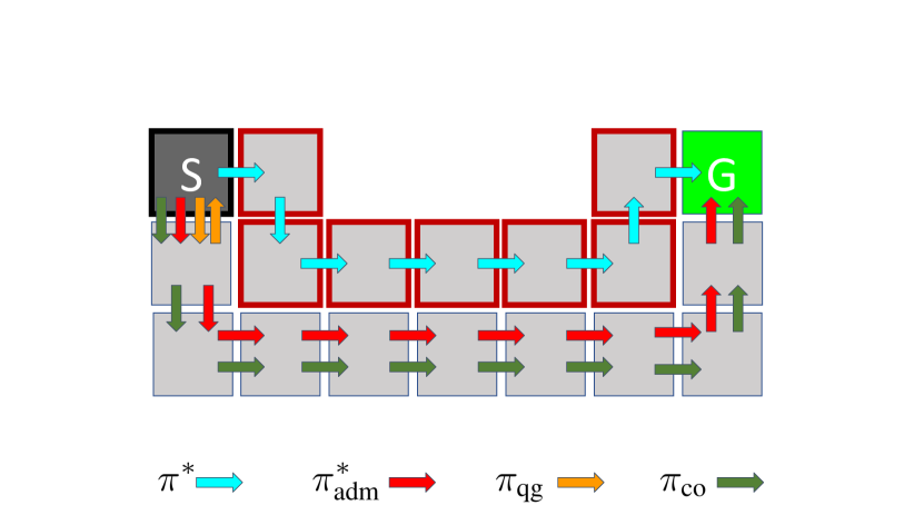
(a) Cliff environment

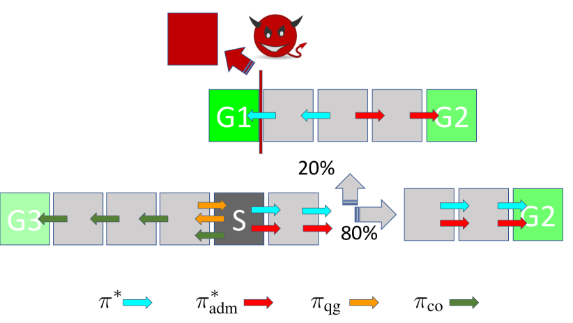
(b) Action hacking environment

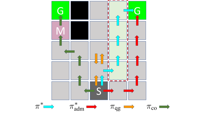
(c) Grass and mud environment

Figure 1: Qualitative assessment. (a) $\pi_{\textnormal{co}}$ is the same as $\pi^{*}_{\textnormal{adm}}$, taking the longer path to the goal state than $\pi^{*}$ in order to avoid the cliff edge, while $\pi_{\textnormal{qg}}$ simply alternates between the starting state and the state below it; (b) $\pi_{\textnormal{co}}$ takes the path to the goal state G3—this behavior is less costly to incentivize than navigating to G2 since in the former case the reward designer mainly needs to compensate for the difference in rewards between G3 and G2 (G1 is reachable only 20% of the time from S); (c) $\pi^{*}$ takes a path through the grass states, $\pi^{*}_{\textnormal{adm}}$ takes a different but admissible path towards the same goal, while $\pi_{\textnormal{co}}$ navigates the agent towards the other goal (with a lower cumulative reward, but the corresponding policy is less costly to force). Quantitative assessment. The objective values of (Computational Challenges) for the approaches based on forcing $\pi^{*}$, $\pi^{*}_{\textnormal{adm}}$, $\pi_{\textnormal{qg}}$, and $\pi_{\textnormal{co}}$ are respectively: (a) $0.27$, $1.59$, $3.93$, and $1.59$; (b) $-2.04$, $14.96$, $5.00$, and $3.82$; and (c) $-9.54$, $9.46$, $17.26$, and $7.92$.

The main blocks of the algorithm are as follows:

• Initialization (lines 1-2). The algorithm selects $\pi^{*}_{\textnormal{adm}}$ as its initial solution, i.e., $\pi_{\textnormal{co}}=\pi^{*}_{\textnormal{adm}}$, and evaluates its cost by approximately solving (Computational Challenges).

• Local search (lines 4-15). Since the initial policy $\pi_{\textnormal{co}}$ is not necessarily cost effective, the algorithm proceeds with a local search in order to find a policy that has a lower value of the objective of (Computational Challenges). In each iteration of the local search procedure, it iterates over all states that are visited by the current $\pi_{\textnormal{co}}$ (i.e., $S^{\pi_{\textnormal{co}}}_{\textnormal{pos}}$), prioritizing those that have a higher value of $Q^{\pi^{*},\overline{R}}(s,\pi^{*}(s))-Q^{\pi^{*},\overline{R}}(s,\pi_{\textnormal{co}}(s))$ (obtained via priority-queue). The intuition behind this prioritization is that this Q value difference is reflective of the cost of forcing action $\pi_{\textnormal{co}}(s)$ (as can be seen by setting $\lambda=0$ in the upper bound of Theorem 4). Hence, deviations from $\pi_{\textnormal{co}}$ that are considered first are deviations from those actions that are expected to induce high cost.

• Evaluating a neighbor solution (lines 7-12). Each visited state $s$ defines a neighbor solution in the local search. To find this neighbor, the algorithm first defines a new admissible set of policies $\Pi^{\prime}$ (line 7), obtained from the current one by making action $\pi_{\textnormal{co}}(s)$ inadmissible. The neighbor solution is then identified as $\pi^{\prime}\in\arg\max_{\pi\in\Pi^{\prime}}{\rho}^{\pi,\overline{R}}$ (line 8) and the costs of forcing it is calculated by approximately solving (Computational Challenges) with ${\pi_{\dagger}}=\pi^{\prime}$ (line 9). If $\pi^{\prime}$ yields a better value of the objective of (Computational Challenges) than $\pi_{\textnormal{co}}$ does (line 10), we have a new candidate policy and the set of admissible policies is updated to $\Pi^{\prime}$ (lines 11-12).

• Returning solution (line 16). Once the local search finishes, the algorithm outputs $\pi_{\textnormal{co}}$ and the reward function $\widehat{R}$ found by approximately solving (Computational Challenges) with ${\pi_{\dagger}}=\pi_{\textnormal{co}}$.

In each iteration of the local search (lines 5-14), the algorithm either finds a new candidate (output${}_{\text{new}}$=true) or the search finishes with that iteration (output${}_{\text{new}}$=false). Notice that the former cannot go indefinitely since the admissible set reduces between two iterations. This means that the algorithm is guaranteed to halt. Since the local search only accepts new policy candidates if they are better than the current $\pi_{\textnormal{co}}$ (line 10), the output of Constrain&Optimize is guaranteed to be better than forcing an optimal admissible policy (i.e., approx. solving (Computational Challenges) with ${\pi_{\dagger}}=\pi^{*}_{\textnormal{adm}}$).

Numerical Simulations

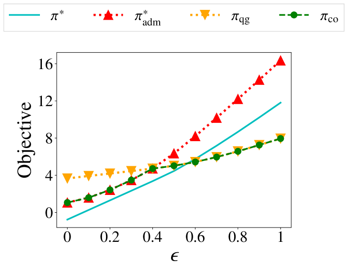
(a) Cliff

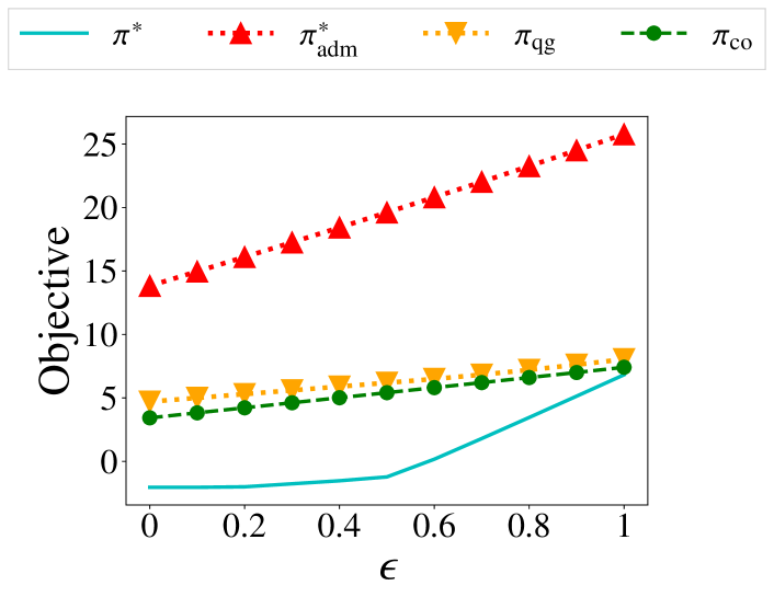
(b) Action hacking

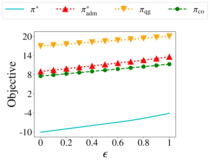
(c) Grass and mud

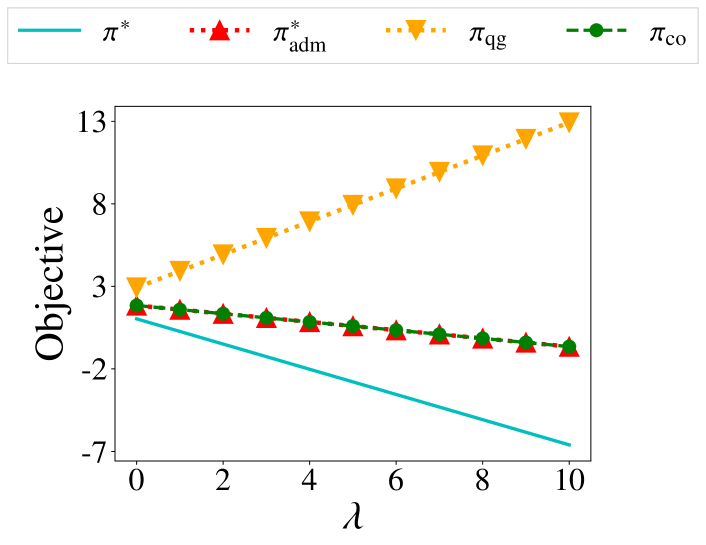
(d) Cliff

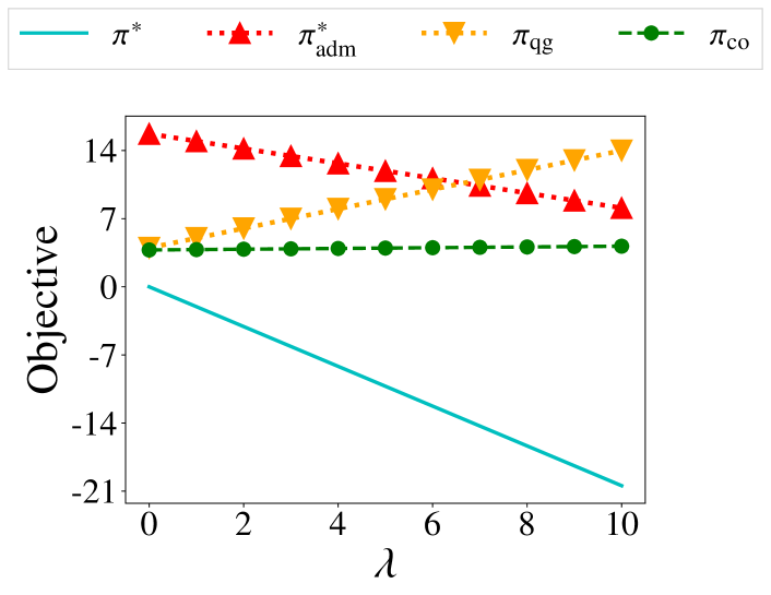
(e) Action hacking

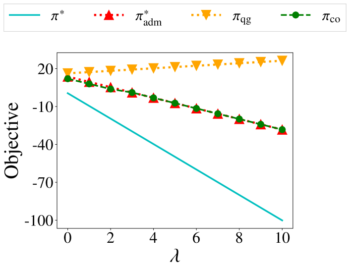
(f) Grass and mud

Figure 2: Effect of $\lambda$ and $\epsilon$ on the objective value of (Computational Challenges) for different approaches. (a, b, c) vary $\epsilon$ with $\lambda=1.0$; (d, e, f) vary $\lambda$ with $\epsilon=0.1$. Lower values on the y-axis denote better performance. Note that $\pi^{*}$ is not an admissible policy in these environments; importantly, the objective value for $\pi_{\textnormal{co}}$ is consistently better (lower) than for $\pi^{*}_{\textnormal{adm}}$ and $\pi_{\textnormal{qg}}$, highlighting its efficacy.

We analyze the efficacy of Constrain&Optimize in solving the optimization problem (Computational Challenges) and the policy it incentivizes, $\pi_{\textnormal{co}}$. We consider three baselines, all based on approximately solving the optimization problem (Computational Challenges), but with different target policies ${\pi_{\dagger}}$: a) forcing an optimal policy, i.e., ${\pi_{\dagger}}=\pi^{*}$, b) forcing an optimal admissible policy, i.e., ${\pi_{\dagger}}=\pi^{*}_{\textnormal{adm}}$, c) forcing the policy obtained by the QGreedy algorithm, i.e., ${\pi_{\dagger}}=\pi_{\textnormal{qg}}$. We compare these approaches by measuring their performance w.r.t. the objective value of (Computational Challenges)—lower value is better. By default, we set the parameters $\gamma=0.9$, $\lambda=1.0$ and $\epsilon=0.1$.

Experimental Testbeds

As an experimental testbed, we consider three simple navigation environments, shown in Figure 1. Each environment contains a start state S and goal state(s) G. Unless otherwise specified, in a non-goal state, the agent can navigate in the left, right, down, and up directions, provided there is a state in that direction. In goal states, the agent has a single action which transports it back to the start state.

Cliff environment (Figure 1(a)). This environment depicts a scenario where some of the states are potentially unsafe due to model uncertainty that the reward designer is aware of. More concretely, the states with “red” cell boundaries in Figure 1(a) represent the edges of a cliff and are unsafe; as such, all actions leading to these states are considered inadmissible. In this environment, the action in the goal state yields a reward $\overline{R}$ of $20$ while all other actions yield a reward $\overline{R}$ of $-1$.

Action hacking environment (Figure 1(b)). This environment depicts a scenario when some of the agent’s actions could be hacked at the deployment phase, taking the agent to a bad state. The reward designer is aware of this potential hacking and seeks to design a reward function so that these actions are inadmissible. More concretely, the action leading the agent to G1 is considered inadmissible. In this environment, we consider the reward function $\overline{R}$ and dynamics $P$ as follows. Whenever an agent reaches any of the goal states (G1, G2, or G3), it has a single action that transports it back to the starting state and yields a reward of $50$, $10$, and $5$ for G1, G2, and G3 respectively. In all other states, the agent can take either the left or right action and navigate in the corresponding direction, receiving a reward of $-1$. With a small probability of $0.20$, taking the right action in the state next to S results in the agent moving up instead of right.

Grass and mud environment (Figure 1(c)). This environment depicts a policy teaching scenario where the reward designer and the agent do not have perfectly aligned preferences (e.g., the agent prefers to walk on grass, which the reward designer wants to preserve). The reward designer wants to incentivize the agent not to step on the grass states, so actions leading to them are considered inadmissible. In addition to the starting state and two goal states, the environment contains four grass states, one mud state, and $16$ ordinary states, shown by “light green”, “light pink”, and “light gray” cells respectively. The “black” cells in the figure represent inaccessible blocks. The reward function $\overline{R}$ is as follows: the action in the goal states yields a reward of $50$; the actions in the grass and mud states yield rewards of $10$ and $-2$ respectively; all other actions have a reward of $-1$.

Results

Figure 1 provides an assessment of different approaches by visualizing the agent’s policies obtained from the designed reward functions $\widehat{R}$. For these results, we set the parameters $\lambda=1.0$ and $\epsilon=0.1$. In order to better understand the effect of the parameters $\lambda$ and $\epsilon$, we vary these parameters and solve (Computational Challenges) with the considered approaches. The results are shown in Figure 2 for each environment separately. We make the following observations based on the experiments. First, the approaches based on forcing $\pi^{*}$ and $\pi^{*}_{\textnormal{adm}}$ benefit more from increasing $\lambda$. This is expected as these two policies have the highest scores under $\overline{R}$; the scores of $\pi_{\textnormal{qg}}$ and $\pi_{\textnormal{co}}$ is less than or equal to the score of $\pi^{*}_{\textnormal{adm}}$. Second, the approaches based on forcing $\pi_{\textnormal{qg}}$ and $\pi_{\textnormal{co}}$ are less susceptible to increasing $\epsilon$. This effect is less obvious, and we attribute it to the fact that QGreedy and Constrain&Optimize output $\pi_{\textnormal{qg}}$ and $\pi_{\textnormal{co}}$ respectively by accounting for the cost of forcing these policies. Since this cost clearly increases with $\epsilon$—intuitively, forcing a larger optimality gap in (Computational Challenges) requires larger reward modifications—we can expect that increasing $\epsilon$ deteriorates more the approaches based on forcing $\pi^{*}$ and $\pi^{*}_{\textnormal{adm}}$. Third, the objective value of (Computational Challenges) is consistently better (lower) for $\pi_{\textnormal{co}}$ than for $\pi^{*}_{\textnormal{adm}}$ and $\pi_{\textnormal{qg}}$, highlighting the relevance of Constrain&Optimize.

Conclusion

The characterization results in this paper showcase the computational challenges of optimal reward design for admissible policy teaching. In particular, we showed that it is computationally challenging to find minimal reward perturbations that would incentivize an optimal agent into adopting a well-performing admissible policy. To address this challenge, we derived a local search algorithm that outperforms baselines which either account for only the agent’s performance or for only the cost of the reward design. On the flip side, this algorithm is only applicable to tabular settings, so one of the most interesting research directions for future work would be to consider its extensions based on function approximation. In turn, this would also make the optimization framework of this paper more applicable to practical applications of interest, such as those related to safe and secure RL.

Appendix A Appendix: Table of Contents

Appendix is structured according to the following sections:

• Section Background introduces additional quantities and lemmas relevant for the formal proofs.

• An approach for solving (Computational Challenges), which is used in the experiments, is provided in Section Approximately Solving the Optimization Problem (). This section also analyzes this approach and provides provable guarantees.

• Section QGreedy Algorithm provides the description of QGreedy and shows that it is sound.

• The proof or Proposition 1 is given in section Proofs of the Results in Section Problem Setup.

• Theorem 1 and Proposition 2 are proven in section Proofs of the Results in Section Computational Challenges and Additional Results. The same section contains an additional hardness result, which proves that the optimization problem (Computational Challenges) is computationally hard.

• Proofs of Lemma 1 and Theorem 2 are in given in section Proofs of the Results from Section Characterization Results for Special MDPs.

• Proofs of Theorem 3 and Theorem 4 are provided in section Proofs of the Results in Section Characterization Results for General MDPs. The same section includes additional results relevant for proving the statements.

Appendix B Background

As explained in the main paper, for a policy $\pi$ and reward function $R$, we define its state-action value function $Q^{\pi,R}$ as

$$Q^{\pi,R}(s,a)=\mathbb{E}\left[\sum_{t=1}^{\infty}\gamma^{t-1}R(s_{t},a_{t})|\pi,s_{1}=s,a_{1}=a\right],$$

where states $s_{t}$ and actions $a_{t}$ are obtained by executing policy $\pi$ starting from state $s_{1}=s$ in which action $a_{1}=a$ is taken.  
The state value function $V^{\pi,R}$ is similarly defined as

$$V^{\pi,R}(s)=\mathbb{E}\left[\sum_{t=1}^{\infty}\gamma^{t-1}R(s_{t},a_{t})|\pi,s_{1}=s\right]=Q^{\pi,R}(s,\pi(s))$$

We define $Q^{*,R}$ and $V^{*,R}$ as the maximum of these values over all policies, i.e.,

$$Q^{*,R}(s,a)=\max_{\pi\in\Pi_{\text{det}}}Q^{\pi,R}(s,a)$$

$$V^{*,R}(s)=\max_{\pi\in\Pi_{\text{det}}}V^{\pi,R}(s)$$

The optimal policy in an MDP can be calculated by setting $\pi(s)\in\operatorname*{arg\,max}_{a}Q^{*,R}(s,a)$ and satisfies $Q^{\pi,R}=Q^{*,R}$. For $R=\overline{R}$, we denote this policy with $\pi^{*}$.  
We define the state occupancy measure ${\mu}^{\pi}$ as

$${\mu}^{\pi}(s)=\mathbb{E}\left[(1-\gamma)\sum_{t=1}^{\infty}\gamma^{t-1}\mathds{1}\left[s_{t}=s\right]|\pi,\sigma\right].$$

${\mu}^{\pi}$ can be efficiently calculated as it is the unique solution to the Bellman flow constraint

$${\mu}^{\pi}(s)=(1-\gamma)\cdot\sigma(s)+\gamma\sum_{s^{\prime}}P(s^{\prime},\pi(s^{\prime}),s){\mu}^{\pi}(s^{\prime}).$$ (2)

An important result that we utilize repeatedly in our proofs, is the following lemma that relates the score difference ${\rho}^{\pi_{1},R}-{\rho}^{\pi_{2},R}$ for two policies $\pi_{1},\pi_{2}$ to their Q-values through the state occupancy measure ${\mu}$.

Lemma 2.

(Schulman et al. 2015) Any two deterministic policies, $\pi_{1}$ and $\pi_{2}$, and reward function $R$ satisfy:

$${\rho}^{\pi_{1},R}-{\rho}^{\pi_{2},R}=\sum_{s\in S}{\mu}^{\pi_{1}}(s)\big{(}Q^{\pi_{2},R}(s,\pi_{1}(s))-Q^{\pi_{2},R}(s,\pi_{2}(s))\big{)}.$$

For a policy $\pi$, we define $S_{\textnormal{pos}}^{\pi}$ as

$$S_{\textnormal{pos}}^{\pi}=\{s|{\mu}^{\pi}(s)>0\}.$$ (3)

We also prove the following lemma, which we use in several results in the following sections.

Lemma 3.

Let $\pi,\pi^{\prime}$ be deterministic policies such that $\pi(s)=\pi^{\prime}(s)$ for all $s\in S_{\textnormal{pos}}^{\pi}\cap S_{\textnormal{pos}}^{\pi^{\prime}}$. Then ${\mu}^{\pi}={\mu}^{\pi^{\prime}}$.

Proof.

Part 1: We first prove a simpler version of the Lemma; we assume that $\pi(s)=\pi^{\prime}(s)$ for all $s\in S_{\textnormal{pos}}^{\pi}$. We then show how to extend the result to the general case.

We prove by induction on $t$ that for all states $s$,

$$\mathbb{P}\left[s_{t}=s|\pi\right]=\mathbb{P}\left[s_{t}=s|\pi^{\prime}\right]$$

where $s_{t}$ denotes the state visited at time $t$.

The claim holds for $t=1$ as the initial probabilities are sampled from $\sigma$. Assuming the claim holds for $t$,

$$\mathbb{P}\left[s_{t}=s|\pi\right] =\sum_{s^{\prime}}\mathbb{P}\left[s_{t-1}=s^{\prime}|\pi\right]\mathbb{P}\left[s^{\prime},\pi(s^{\prime}),s\right]$$

$$=\sum_{s^{\prime}:\mathbb{P}\left[s_{t-1}=s^{\prime}|\pi\right]>0}\mathbb{P}\left[s_{t-1}=s^{\prime}|\pi\right]\mathbb{P}\left[s^{\prime},\pi(s^{\prime}),s\right]$$

$$\overset{(i)}{=}\sum_{s^{\prime}:\mathbb{P}\left[s_{t-1}=s^{\prime}|\pi\right]>0}\mathbb{P}\left[s_{t-1}=s^{\prime}|\pi^{\prime}\right]\mathbb{P}\left[s^{\prime},\pi(s^{\prime}),s\right]$$

$$\overset{(ii)}{=}\sum_{s^{\prime}:\mathbb{P}\left[s_{t-1}=s^{\prime}|\pi\right]>0}\mathbb{P}\left[s_{t-1}=s^{\prime}|\pi^{\prime}\right]\mathbb{P}\left[s^{\prime},\pi^{\prime}(s^{\prime}),s\right]$$

$$\leq\sum_{s^{\prime}}\mathbb{P}\left[s_{t-1}=s^{\prime}|\pi^{\prime}\right]\mathbb{P}\left[s^{\prime},\pi^{\prime}(s^{\prime}),s\right]$$

$$=\mathbb{P}\left[s_{t}=s|\pi^{\prime}\right],$$

where $(i)$ follows from the induction hypotheses and $(ii)$ follows from the fact that if $\mathbb{P}\left[s_{t-1}=s^{\prime}|\pi\right]>0$, then ${\mu}^{\pi}(s^{\prime})>0$ and therefore $\pi(s)=\pi^{\prime}(s)$. Since

$$\sum_{s}\mathbb{P}\left[s_{t}=s|\pi\right]=\sum_{s}\mathbb{P}\left[s_{t}=s|\pi^{\prime}\right]=1,$$

it follows that

$$\mathbb{P}\left[s_{t}=s|\pi\right]=\mathbb{P}\left[s_{t}=s|\pi^{\prime}\right].$$

Therefore,

$${\mu}^{\pi}(s)=\sum_{t=1}^{\infty}\mathbb{P}\left[s_{t}=s|\pi\right]=\sum_{t=1}^{\infty}\mathbb{P}\left[s_{t}=s|\pi^{\prime}\right]={\mu}^{\pi^{\prime}}(s).$$

Part 2: Now, in order to obtain the general case, define $\tilde{\pi}$ as follows.

$$\tilde{\pi}(s):=\begin{cases}\pi(s)\quad&\text{if}\quad s\in S_{\textnormal{pos}}^{\pi}\\ \pi^{\prime}(s)\quad&\text{otherwise}\end{cases},$$

By the simpler version just proved, since $\tilde{\pi}(s)=\pi(s)$ for all $s\in S_{\textnormal{pos}}^{\pi}$, ${\mu}^{\tilde{\pi}}={\mu}^{\pi}$.  
Furthermore, for all $s\in S_{\textnormal{pos}}^{\pi^{\prime}}$, either $s\in S_{\textnormal{pos}}^{\pi}$, in which case $\pi(s)=\pi^{\prime}(s)$ by assumption and therefore by definition of $\tilde{\pi}=\pi(s)=\pi^{\prime}(s)$, or $s\notin S_{\textnormal{pos}}^{\pi}$, in which case, $\tilde{\pi}(s)=\pi^{\prime}(s)$. Since $\tilde{\pi}(s)=\pi^{\prime}(s)$ in both cases, it follows that by the simpler version just proved, ${\mu}^{\tilde{\pi}}={\mu}^{\pi^{\prime}}$.  
Therefore ${\mu}^{\pi}={\mu}^{\tilde{\pi}}={\mu}^{\pi^{\prime}}$ as claimed. ∎

Appendix C Approximately Solving the Optimization Problem (Computational Challenges)

In this section, we show to efficiently approximate the optimization problem (Computational Challenges). In order to obtain the approximate solution, we will consider the following optimization problem

$$\min_{R}\quad \left\lVert R-\overline{R}\right\rVert_{2}$$ (P5-ATK)

s.t. $$\forall s,a:Q(s,a)=R(s,a)+\gamma\sum_{s^{\prime}}P(s,a,s^{\prime})V(s^{\prime})$$ (4)

$$\forall s\in S_{\textnormal{pos}}^{\pi_{\dagger}},a\neq{\pi_{\dagger}}(s):Q(s,{\pi_{\dagger}}(s))\geq Q(s,a)+\epsilon^{\prime}(s,a)$$ (5)

$$\forall s\in S_{\textnormal{pos}}^{\pi_{\dagger}}:V(s)=Q(s,{\pi_{\dagger}}(s))$$ (6)

$$\forall s\notin S_{\textnormal{pos}}^{\pi_{\dagger}},a:V(s)\geq Q(s,a),$$ (7)

where $\epsilon^{\prime}(s,a)\geq 0$ are arbitrary non-negative values that will be specified later. We first show that the constraints of the optimization problem effectively ensure that $V$ and $Q$ can be thought of as the $V^{*,R}$ and $Q^{*,R}$ vectors respectively. Note that this is not trivial since for $s\notin S_{\textnormal{pos}}^{\pi_{\dagger}}$, the constraint $V(s)=\max_{a}Q(s,a)$ is not explicitly enforced. Formally, we have the following lemma.

Lemma 4.

Let $\epsilon^{\prime}(s,a)$ be a non-negative vector. If the vectors $(R,Q,V)$ satisfy the constraints of the optimization problem (P5-ATK), the vectors $(R,Q^{*,R},V^{*,R})$ satisfy the constraints as well.

Proof.

Starting with $Q,V$, we run the standard value iteration algorithm for finding $Q^{*,R},V^{*,R}$ and claim that at the end of each step, all the constraints would still be satisfied. Concretly, We set $V^{0}=V$ and $Q^{0}=Q$ and for all $t\geq 0$:

$$V^{t+1}(s,a)=\max_{a}Q^{t}(s,a)$$

$$Q^{t+1}(s,a)=R(s,a)+\gamma\sum_{s^{\prime}}P(s,a,s^{\prime})V^{t+1}(s^{\prime}).$$

We claim that for all $t\geq 0$, the vectors $(R,Q^{t},V^{t})$ satisfty the constraints (4) to (7). We prove that claim by induction on $t$.

For $t=0$, the claim holds by assumption. Assume that the claim holds for $t-1$; we will show that it holds for $t$ as well by proving the constraints (4), (6), (5) and (7) repsectively. Constraint (4) holds by definition of $Q^{t}(s,a)$. For constraint (6), observe that for all $s\in S_{\textnormal{pos}}^{\pi_{\dagger}}$,

$$V^{t}(s) \overset{(i)}{=}\max_{a}Q^{t-1}(s,a)$$

$$\overset{(ii)}{=}Q^{t-1}(s,{\pi_{\dagger}}(s))$$

$$\overset{(iii)}{=}V^{t-1}(s)$$ (8)

where $(i)$ follows from the definition of $V^{t}$, $(ii)$ follows from (5) and $(iii)$ follows from (6) for $V^{t-1}$ and $Q^{t-1}$.

Now observe that if $s\in S_{\textnormal{pos}}^{\pi_{\dagger}}$ and $s^{\prime}\notin S_{\textnormal{pos}}^{\pi_{\dagger}}$, then $P(s,{\pi_{\dagger}}(s),s^{\prime})=0$ as otherwise given (2), ${\mu}^{\pi_{\dagger}}(s^{\prime})$ would be lower bounded by ${\mu}^{\pi_{\dagger}}(s)\cdot P(s,{\pi_{\dagger}}(s),s^{\prime})>0$, contradicting the assumption $s^{\prime}\notin S_{\textnormal{pos}}^{{\pi_{\dagger}}}$. Therefore, for all $s\in S_{\textnormal{pos}}^{\pi_{\dagger}}$,

$$Q^{t}(s,{\pi_{\dagger}}(s)) =R(s,{\pi_{\dagger}}(s))+\gamma\sum_{s^{\prime}}P(s,{\pi_{\dagger}}(s),s^{\prime})V^{t}(s^{\prime}).$$

$$=R(s,{\pi_{\dagger}}(s))+\gamma\sum_{s^{\prime}\in S_{\textnormal{pos}}^{\pi_{\dagger}}}P(s,{\pi_{\dagger}}(s),s^{\prime})V^{t}(s^{\prime}).$$

$$\overset{(i)}{=}R(s,{\pi_{\dagger}}(s))+\gamma\sum_{s^{\prime}\in S_{\textnormal{pos}}^{\pi_{\dagger}}}P(s,{\pi_{\dagger}}(s),s^{\prime})V^{t-1}(s^{\prime}).$$

$$=R(s,{\pi_{\dagger}}(s))+\gamma\sum_{s^{\prime}}P(s,{\pi_{\dagger}}(s),s^{\prime})V^{t-1}(s^{\prime}).$$

$$=Q^{t-1}(s,{\pi_{\dagger}}(s)),$$ (9)

where $(i)$ follows from (8). Together with (8), (9) implies that the constraint (6) still holds.

Now observe that for $s\notin S_{\textnormal{pos}}^{\pi_{\dagger}}$,

$$V^{t}(s)=\max_{a}Q^{t-1}(s,a)\leq V^{t-1}(s),$$

where the inequality follows from the induction hypothesis; namely, constraint (7) for $V^{t-1}$ and $Q^{t-1}$. This means that for all $s$ (both when $s\notin S_{\textnormal{pos}}^{\pi_{\dagger}}$ and when $s\in S_{\textnormal{pos}}^{\pi_{\dagger}}$), $V^{t}(s)\leq V^{t-1}(s)$ and therefore given (4),

$$Q^{t}(s,a)\leq Q^{t-1}(s,a).$$

for all $s,a$. This implies that the constraint (5) still holds because the LHS has stayed the same and RHS hasn’t increased. Finally, constraint (7) holds as well because it holds with $V^{t},Q^{t-1}$ by definition of $V^{t}$ and $Q^{t}(s,a)\leq Q^{t-1}(s,a)$.

Since $(Q^{t},V^{t})$ converge to $(Q^{*,R},V^{*,R})$ and the constraints characterize a closed set, $(R,Q^{*,R},V^{*,R})$ also satisfy the constraints. ∎

While the value of $\epsilon^{\prime}$ can be arbitrary in (5), in our analysis we will mainly consider $\epsilon^{\prime}_{{\pi_{\dagger}}}$, which for a non-negative number $\epsilon\geq 0$ and policy ${\pi_{\dagger}}$ we define as

$${\epsilon^{\prime}_{{\pi_{\dagger}}}(\tilde{s},\tilde{a})}:=\begin{cases}\dfrac{\epsilon}{\min_{\pi\in D({\pi_{\dagger}},\tilde{s},\tilde{a})}{\mu}^{\pi}(\tilde{s})}\quad&\text{if}\quad\tilde{s}\in S_{\textnormal{pos}}^{\pi_{\dagger}}\text{ and }\tilde{a}\neq\pi(s)\\ 0\quad&\text{otherwise}.\end{cases},$$ (10)

where

$$D({\pi_{\dagger}},\tilde{s},\tilde{a})=\big{\{}\pi:\pi(\tilde{s})=\tilde{a}\text{ and }\pi(s)={\pi_{\dagger}}(s)\text{ for all }s\in S_{\textnormal{pos}}^{\pi_{\dagger}}\backslash\{\tilde{s}\}\big{\}}.$$

Of course, in order for the above definition to be valid, we need to ensure that the denominator is non-zero, i.e. $\min_{\pi\in D({\pi_{\dagger}},\tilde{s},\tilde{a})}{\mu}^{\pi}(\tilde{s})>0$. The following lemma ensures that this is the case.

Lemma 5.

Let ${\pi_{\dagger}}\in\Pi_{\text{det}}$ be a deterministic policy. Define $S_{\textnormal{pos}}^{\pi_{\dagger}}$ as in (3). Let $\tilde{s}$ be an arbitrary state in $S_{\textnormal{pos}}^{\pi_{\dagger}}$ and $\pi$ be a deterministic policy such that

$$\pi(s)={\pi_{\dagger}}(s)\quad\text{ for all }\quad s\in S_{\textnormal{pos}}^{\pi_{\dagger}}\backslash\{\tilde{s}\}.$$

Then

$${\mu}^{\pi}(\tilde{s})>0.$$

Proof.

Assume that this is not the case and ${\mu}^{\pi}(\tilde{s})=0$. Then $s\notin S_{\textnormal{pos}}^{\pi}$ and therefore $\pi(s)={\pi_{\dagger}}(s)$ for all $S_{\textnormal{pos}}^{{\pi_{\dagger}}}\cap S_{\textnormal{pos}}^{\pi}$. Lemma 3 (from section Background) implies that ${\mu}^{\pi}={\mu}^{{\pi_{\dagger}}}$ which is a contradiction since ${\mu}^{{\pi_{\dagger}}}(s)>0={\mu}^{\pi}(\tilde{s})$. Therefore the initial assumption was wrong and ${\mu}^{\pi}(s)>0$. ∎

Proposition 3.

Let $\epsilon$ be a non-negative number. Denote by $\widehat{R}^{{\pi_{\dagger}}}$ the solution of the optimization problem (Computational Challenges) and let $\widehat{R}^{\prime}$ be the solution to (P5-ATK) with $\epsilon^{\prime}=\epsilon^{\prime}_{{\pi_{\dagger}}}$ where $\epsilon^{\prime}_{{\pi_{\dagger}}}$ is defined as in Equation (10). Then $\widehat{R}^{\prime}$ satisfies the constraints of (Computational Challenges) and

$$0\leq\left\lVert\widehat{R}^{\prime}-\overline{R}\right\rVert_{2}-\left\lVert\widehat{R}^{{\pi_{\dagger}}}-\overline{R}\right\rVert_{2}\leq\left\lVert\epsilon^{\prime}\right\rVert_{2}$$

Proof.

Before we proceed with the proof, note that $\min_{\pi\in D({\pi_{\dagger}},\tilde{s},\tilde{a})}{\mu}^{\pi}(\tilde{s})>0$ because of Lemma 5.  
Part 1: We first prove that $\widehat{R}^{\prime}$ satisfies the constraints of (Computational Challenges), which automatically proves the left inequality by optimality of $\widehat{R}^{{\pi_{\dagger}}}$. Set $Q=Q^{*,\widehat{R}^{\prime}}$ and $V=V^{*,\widehat{R}^{\prime}}$. Given Lemma 4, $(R,Q,V)$ satisfy the constraints of (P5-ATK). Define $\tilde{\pi}_{\dagger}\in\Pi_{\text{det}}$ as

$$\tilde{\pi}_{\dagger}(s)=\operatorname*{arg\,max}Q(s,a).$$ (11)

It is clear that $Q^{\tilde{\pi}_{\dagger},\widehat{R}^{\prime}}=Q$. Now note that since $\operatorname*{arg\,max}Q(s,a)={\pi_{\dagger}}(s)$ for all states $s\in S_{\textnormal{pos}}^{\pi_{\dagger}}$, Lemma 2 implies that

$${\rho}^{{\pi_{\dagger}},\widehat{R}^{\prime}}-{\rho}^{\tilde{\pi}_{\dagger},\widehat{R}^{\prime}} =\sum_{s}{\mu}^{{\pi_{\dagger}}}(s)\big{(}Q(s,{\pi_{\dagger}}(s))-Q(s,\tilde{\pi}_{\dagger}(s))\big{)}$$

$$=\sum_{s\in S_{\textnormal{pos}}^{\pi_{\dagger}}}{\mu}^{{\pi_{\dagger}}}(s)\big{(}Q(s,{\pi_{\dagger}}(s))-Q(s,\tilde{\pi}_{\dagger}(s))\big{)}$$

$$=0.$$

Given this, it suffices to prove that

$${\rho}^{\tilde{\pi}_{\dagger}}\geq{\rho}^{\pi}+\epsilon\quad\text{if}\quad\exists s\in S_{\textnormal{pos}}^{\pi_{\dagger}}:\pi(s)\neq{\pi_{\dagger}}(s),$$

Our proof now proceeds in a similar fashion to the proof of Lemma 1 in (Rakhsha et al. 2020b): We start by proving the claim policies that effectively, differ from ${\pi_{\dagger}}$ in only a single state. We then generalise the claim for other policies via induction.

Concretely, we first claim that if $\pi\in D({\pi_{\dagger}},\tilde{s},\tilde{a})$ for some $\tilde{s}\in S_{\textnormal{pos}}^{\pi_{\dagger}}$ and $\tilde{a}$, then ${\rho}^{\tilde{\pi}_{\dagger},\widehat{R}^{\prime}}-{\rho}^{\pi,\widehat{R}^{\prime}}\geq\epsilon$. To see why, note that

$${\rho}^{\tilde{\pi}_{\dagger},\widehat{R}^{\prime}}-{\rho}^{\pi,\widehat{R}^{\prime}} =\sum_{s}{\mu}^{\pi}(s)\big{(}Q(s,\tilde{\pi}_{\dagger}(s))-Q(s,\pi(s)\big{)}$$

$$={\mu}^{\pi}(\tilde{s})\big{(}Q(\tilde{s},\tilde{\pi}_{\dagger}(\tilde{s}))-Q(\tilde{s},\pi(\tilde{s})\big{)}+\sum_{s\neq\tilde{s}}{\mu}^{\pi}(s)\big{(}Q(s,\tilde{\pi}_{\dagger}(s))-Q(s,\pi(s)\big{)}$$

$$\overset{(i)}{\geq}{\mu}^{\pi}(\tilde{s})\big{(}Q(\tilde{s},\tilde{\pi}_{\dagger}(\tilde{s}))-Q(\tilde{s},\pi(\tilde{s})\big{)}$$

$$\overset{(ii)}{\geq}{\mu}^{\pi}(\tilde{s})\epsilon^{\prime}(\tilde{s},\pi(\tilde{s}))$$

$$\overset{(iii)}{\geq}\epsilon.$$

where $(i)$ follows from the definition of $\tilde{\pi}_{\dagger}$, $(ii)$ follows from (5) since $\tilde{s}\in S_{\textnormal{pos}}^{\pi_{\dagger}}$ and $(iii)$ follows from the definition of $\epsilon^{\prime}_{{\pi_{\dagger}}}$ in (10).

We now generalize the above result by showing that if $\pi$ is a policy such that there exists state $\tilde{s}\in S_{\textnormal{pos}}^{\pi_{\dagger}}$ satisfying $\pi(\tilde{s})\neq{\pi_{\dagger}}(\tilde{s})$, then ${\rho}^{\tilde{\pi}_{\dagger},\widehat{R}^{\prime}}-{\rho}^{\pi,\widehat{R}^{\prime}}\geq\epsilon$. We do this by induction on $d_{S_{\textnormal{pos}}^{\pi_{\dagger}}}(\pi,{\pi_{\dagger}})$ where we define $d_{\tilde{S}}(\pi,\pi^{\prime})$ for $\tilde{S}\subseteq S$ as

$$d_{\tilde{S}}(\pi,\pi^{\prime}):=\left|\left\{s\in\tilde{S}:\pi(s)\neq\pi^{\prime}(s)\right\}\right|.$$

For $d_{S_{\textnormal{pos}}^{\pi_{\dagger}}}(\pi,{\pi_{\dagger}})=1$, the claim is already proved since this is equivalent to $\pi\in D({\pi_{\dagger}},\tilde{s},\tilde{a})$ for some $\tilde{s}\in S_{\textnormal{pos}}^{\pi_{\dagger}}$ and $\tilde{a}$. Suppose the claim holds for all $\pi$ satisfying $d_{S_{\textnormal{pos}}^{\pi_{\dagger}}}(\pi,{\pi_{\dagger}})\leq k$ where $k\geq 1$. We prove it holds for all $\pi$ satisfying $d_{S_{\textnormal{pos}}^{\pi_{\dagger}}}(\pi,{\pi_{\dagger}})=k+1$. Let $\pi$ be one such policy and note that by Lemma 2,

$${\rho}^{\tilde{\pi}_{\dagger},\widehat{R}^{\prime}}-{\rho}^{\pi,\widehat{R}^{\prime}} =\sum_{s}{\mu}^{\pi}(s)\big{(}Q(s,\tilde{\pi}_{\dagger}(s))-Q(s,\pi(s)\big{)}\geq 0.$$

On the other hand, again by Lemma 2,

$${\rho}^{\tilde{\pi}_{\dagger},\widehat{R}^{\prime}}-{\rho}^{\pi,\widehat{R}^{\prime}} =\sum_{s}{\mu}^{\tilde{\pi}_{\dagger}}(s)\big{(}Q^{\pi,\widehat{R}^{\prime}}(s,\tilde{\pi}_{\dagger}(s))-Q^{\pi,\widehat{R}^{\prime}}(s,\pi(s))\big{)}$$

$$=\sum_{s\in S_{\textnormal{pos}}^{\tilde{\pi}_{\dagger}}}{\mu}^{\tilde{\pi}_{\dagger}}(s)\big{(}Q^{\pi,\widehat{R}^{\prime}}(s,\tilde{\pi}_{\dagger}(s))-Q^{\pi,\widehat{R}^{\prime}}(s,\pi(s))\big{)}.$$

$$\overset{(i)}{=}\sum_{s\in S_{\textnormal{pos}}^{\pi_{\dagger}}}{\mu}^{\tilde{\pi}_{\dagger}}(s)\big{(}Q^{\pi,\widehat{R}^{\prime}}(s,\tilde{\pi}_{\dagger}(s))-Q^{\pi,\widehat{R}^{\prime}}(s,\pi(s))\big{)}.$$

Where $(i)$ follows from the fact that $S_{\textnormal{pos}}^{\pi_{\dagger}}=S_{\textnormal{pos}}^{\tilde{\pi}_{\dagger}}$ by Lemma 3. Therefore, there exists a state $s\in S_{\textnormal{pos}}^{\pi_{\dagger}}$ such that

$$Q^{\pi,\widehat{R}^{\prime}}(s,\tilde{\pi}_{\dagger}(s))-Q^{\pi,\widehat{R}^{\prime}}(s,\pi(s))\geq 0.$$

Define the policy $\tilde{\pi}$ as

$$\tilde{\pi}(\tilde{s})=\begin{cases}{\pi_{\dagger}}(\tilde{s})\quad&\text{if}\quad\tilde{s}=s\\ \pi(\tilde{s})\quad&\text{otherwise}\end{cases}.$$

It follows that

$${\rho}^{\tilde{\pi},\widehat{R}^{\prime}}-{\rho}^{\pi,\widehat{R}^{\prime}}={\mu}^{\tilde{\pi}}(s)\big{(}Q^{\pi,\widehat{R}^{\prime}}(s,\tilde{\pi}_{\dagger}(s))-Q^{\pi,\widehat{R}^{\prime}}(s,\pi(s))\big{)}\geq 0.$$

However, $d_{S_{\textnormal{pos}}^{\pi_{\dagger}}}({\pi_{\dagger}},\tilde{\pi})\leq k-1$ and therefore

$${\rho}^{\tilde{\pi}_{\dagger},\widehat{R}^{\prime}}-{\rho}^{\tilde{\pi},\widehat{R}^{\prime}}\geq\epsilon.$$

Which proves the claim.

Part 2: For the right inequality, define $\widehat{R}"$ as $\widehat{R}":=\widehat{R}^{{\pi_{\dagger}}}-\epsilon^{\prime}_{{\pi_{\dagger}}}$. We claim that

$${\pi_{\dagger}}(s)\in\operatorname*{arg\,max}_{a}Q^{*,\widehat{R}^{{\pi_{\dagger}}}}(s,a)\quad\text{for all}\quad s\in S_{\textnormal{pos}}^{\pi_{\dagger}}.$$ (12)

To prove this, define $\tilde{\pi}_{\dagger}\in\Pi_{\text{det}}$ as

$$\tilde{\pi}_{\dagger}(s)=\operatorname*{arg\,max}_{a}Q^{*,\widehat{R}^{{\pi_{\dagger}}}}(s,a).$$

Now note that

$$0 \overset{(i)}{=}{\rho}^{{\pi_{\dagger}},\widehat{R}^{{\pi_{\dagger}}}}-{\rho}^{\tilde{\pi}_{\dagger},\widehat{R}^{{\pi_{\dagger}}}}$$

$$=\sum_{s}{\mu}^{\pi_{\dagger}}(s)\cdot\left(Q^{\tilde{\pi}_{\dagger},\widehat{R}^{{\pi_{\dagger}}}}(s,{\pi_{\dagger}}(s))-Q^{\tilde{\pi}_{\dagger},\widehat{R}^{{\pi_{\dagger}}}}(s,\tilde{\pi}_{\dagger}(s))\right)$$

$$\overset{(ii)}{=}\sum_{s}{\mu}^{\pi_{\dagger}}(s)\cdot\left(Q^{*,\widehat{R}^{{\pi_{\dagger}}}}(s,{\pi_{\dagger}}(s))-Q^{*,\widehat{R}^{{\pi_{\dagger}}}}(s,\tilde{\pi}_{\dagger}(s))\right)$$

where $(i)$ follows from optimality of ${\pi_{\dagger}}$ in $\widehat{R}^{{\pi_{\dagger}}}$ and $(ii)$ follows from the fact that $Q^{*,\widehat{R}^{\pi_{\dagger}}}=Q^{\tilde{\pi}_{\dagger},\widehat{R}^{{\pi_{\dagger}}}}$. Therefore $Q^{*,\widehat{R}^{{\pi_{\dagger}}}}(s,{\pi_{\dagger}}(s))=Q^{*,\widehat{R}^{{\pi_{\dagger}}}}(s,\tilde{\pi}_{\dagger}(s))$ for all $s\in S_{\textnormal{pos}}^{\pi_{\dagger}}$ which is equivalent to (12).

Given this result, we further assume that $\tilde{\pi}_{\dagger}(s)={\pi_{\dagger}}(s)$ for all $s\in S_{\textnormal{pos}}^{\pi_{\dagger}}$ since we did not originially specify how to break ties in the definition of $\tilde{\pi}_{\dagger}$. This also implies $S_{\textnormal{pos}}^{{\pi_{\dagger}}}=S_{\textnormal{pos}}^{\tilde{\pi}_{\dagger}}$ since ${\mu}^{{\pi_{\dagger}}}={\mu}^{\tilde{\pi}_{\dagger}}$ by Lemma 3.

Now note that given the construction of $\widehat{R}"$,

$$Q^{\tilde{\pi}_{\dagger},\widehat{R}^{{\pi_{\dagger}}}}(s,\tilde{\pi}_{\dagger}(s))=Q^{\tilde{\pi}_{\dagger},\widehat{R}"}(s,\tilde{\pi}_{\dagger}(s))$$

for all $s$. This is because the rewards for the state-action pairs $(s,\tilde{\pi}_{\dagger}(s))$ were not modified. Since no reward has increased, this further implies that $V^{\tilde{\pi}_{\dagger},\widehat{R}"}=V^{\tilde{\pi}_{\dagger},\widehat{R}^{{\pi_{\dagger}}}}$. Now note that for all $s,a$,

$$Q^{\tilde{\pi}_{\dagger},\widehat{R}"}(s,a)-Q^{\tilde{\pi}_{\dagger},\widehat{R}^{{\pi_{\dagger}}}}(s,a) =\widehat{R}"(s,a)-\widehat{R}^{{\pi_{\dagger}}}(s,a)\leq-\epsilon^{\prime}(s,a)\cdot\mathds{1}\left[s\in S_{\textnormal{pos}}^{{\pi_{\dagger}}}\right]$$

Recall however that by definition of $\tilde{\pi}_{\dagger}$,

$$Q^{\tilde{\pi}_{\dagger},\widehat{R}^{{\pi_{\dagger}}}}(s,\tilde{\pi}_{\dagger}(s))\geq Q^{\tilde{\pi}_{\dagger},\widehat{R}^{{\pi_{\dagger}}}}(s,a).$$

We can therefore conclude that

$$Q^{\tilde{\pi}_{\dagger},\widehat{R}"}(s,\tilde{\pi}_{\dagger}(s))\geq Q^{\tilde{\pi}_{\dagger},\widehat{R}"}(s,a)+\epsilon^{\prime}(s,a)\cdot\mathds{1}\left[s\in S_{\textnormal{pos}}^{{\pi_{\dagger}}}\right].$$

This means that $\left(R=\widehat{R}",Q=Q^{\tilde{\pi}_{\dagger},\widehat{R}"},V=V^{\tilde{\pi}_{\dagger},\widehat{R}"},{\pi_{\dagger}}=\tilde{\pi}_{\dagger}\right)$ satisfy all of the constraints of (P5-ATK). Since ${\pi_{\dagger}}(s)=\tilde{\pi}_{\dagger}(s)$ for all $s\in S_{\textnormal{pos}}^{{\pi_{\dagger}}}$, this means that $\left(R=\widehat{R}",Q=Q^{\tilde{\pi}_{\dagger},\widehat{R}"},V=V^{\tilde{\pi}_{\dagger},\widehat{R}"},{\pi_{\dagger}}={\pi_{\dagger}}\right)$ satisfy the constraints of (P5-ATK) as well. Therefore, by optimality of $\widehat{R}^{\prime}$,

$$\left\lVert\overline{R}-\widehat{R}^{\prime}\right\rVert_{2} \leq\left\lVert\overline{R}-\widehat{R}"\right\rVert_{2}$$

$$\leq\left\lVert\overline{R}-\widehat{R}^{{\pi_{\dagger}}}\right\rVert_{2}+\left\lVert\widehat{R}^{{\pi_{\dagger}}}-\widehat{R}"\right\rVert_{2}$$

$$=\left\lVert\overline{R}-\widehat{R}^{{\pi_{\dagger}}}\right\rVert_{2}+\left\lVert\epsilon^{\prime}\right\rVert_{2}.$$

∎

Appendix D QGreedy Algorithm

In this section, we present the QGreedy algorithm and prove its correctness. Recall that this algorithm finds a solution to the optimization problem:

$${\Delta_{Q}}=\min_{\pi\in\Pi^{\textnormal{adm}}_{\textnormal{det}}}\max_{s\in S_{\textnormal{pos}}^{\pi}}\big{(}Q^{*,\overline{R}}(s,\pi^{*}(s))-Q^{*,\overline{R}}(s,\pi(s))\big{)}.$$

The intuition behind the QGreedy algorithm as follows. It starts by finding the state $s$ which has the highest value of $\delta(s)=\min_{a\in A_{s}^{\textnormal{adm}}}Q^{*,\overline{R}}(s,\pi^{*}(s))-Q^{*,\overline{R}}(s,a)$ among admissible state-action pairs—this value provides an upper bound on ${\Delta_{Q}}$ and is tight if $s$ is reachable by any admissible policy. If this is not the case, then there might exists a policy $\pi$ which results in lower value of ${\Delta_{Q}^{\pi}}$ by not reaching $s$ (making ${\mu}^{\pi}(s)=0$). Therefore, after finding $s$, the algorithm proceeds by finding the set of state-action pairs that are “connected” to $s$ in that policies defined on these pairs reach $s$ with strictly positive probability. These state action pairs are removed from the admissible set of state-action pairs, and the algorithm proceeds with the next iteration. The output is defined by the minimum of all of the gaps $\delta$ found in each iteration, and the policy can be reconstructed from the set of state-action pairs that are “connected” to the state that defines this gap.  
The pseudo-code of QGreedy can be found in Algorithm 2 and provides a more detailed description of the algorithm.

Algorithm 2 QGreedy

Input: MDP $\overline{M}$, admissible action set $A_{s}^{\textnormal{adm}}$ for each state $s$.
Output: ${\Delta_{Q}}$, Policy $\pi\in\operatorname*{arg\,min}_{\pi}\Delta_{Q}^{\pi}$.

1:  Calculate Q-values $Q^{*,\overline{R}}$.

2:  Let $\pi^{*}(s)=\max_{a}Q^{*,\overline{R}}(s,a)$.

3:  Let $\text{ADM}^{(0)}=\{(s,a)|a\in A_{s}^{\textnormal{adm}}\}$.

4:  Let $\tilde{S}^{(0)}=S$.

5:  Let $S_{\sigma}=\{s|\sigma(s)\neq 0\}$.

6:  Let $t=0$.

7:  while $S_{\sigma}\subseteq\tilde{S}^{(t)}$ do

8:     Let $\text{ADM}^{(t)}_{s}=\{a|(s,a)\in\text{ADM}^{(t)}\}$ for all $s\in\tilde{S}^{(t)}$.

9:     Let $\delta^{(t)}(s)=\min_{a\in\text{ADM}_{s}^{(t)}}Q^{*,\overline{R}}(s,\pi^{*}(s))-Q^{*,\overline{R}}(s,a)$ for all $s\in\tilde{S}^{(t)}$.

10:     Let $s_{t}=\operatorname*{arg\,max}_{s\in\tilde{S}^{(t)}}\delta^{(t)}(s)$ and $\Delta_{t}=\delta^{(t)}(s_{t})$.

11:     Let $\pi_{t}(s)=\operatorname*{arg\,min}_{a\in\text{ADM}_{s}^{(t)}}Q^{*,\overline{R}}(s,\pi^{*}(s))-Q^{*,\overline{R}}(s,a)$ for all $s\in\tilde{S}^{(t)}$ and choose $\pi_{t}(s)$ arbitrarily otherwise.

12:     Let $\tilde{S}^{(t+1)}=\tilde{S}^{(t)}$ and $\text{ADM}^{(t+1)}=\text{ADM}^{(t)}$.

13:     Let $S_{\delta}=\{s_{t}\}$

14:     while $S_{\delta}\neq\emptyset$ do

15:        $\tilde{S}^{(t+1)}=\tilde{S}^{(t+1)}\backslash S_{\delta}$.

16:        $\text{ADM}^{(t+1)}=\text{ADM}^{(t+1)}\backslash\{(s,a)|P(s,a,\tilde{s})>0\text{ for some }\tilde{s}\notin\tilde{S}^{(t+1)}\}$.

17:        Let $S_{\delta}=\{s\in\tilde{S}^{(t+1)}|(s,a)\notin\text{ADM}^{(t+1)}\text{ for all }a\}$

18:     end while

19:     $t=t+1$.

20:  end while

21:  Let $t^{*}=\operatorname*{arg\,min}_{t}\Delta_{t}$

22:  return $\Delta_{t^{*}},\pi_{t^{*}}$

The following result formally shows that QGreedy outputs a correct result.

Lemma 6.

Let $\Delta_{A},\pi_{A}$ denote the output of the algorithm 2. Then it holds that

$${\Delta_{Q}}=\Delta_{A}=\Delta_{Q}^{\pi_{A}},$$

where $\Delta_{Q}^{\pi}$ is defined as

$${\Delta_{Q}^{\pi}}=\max_{s\in S_{\textnormal{pos}}^{\pi}}\left(Q^{*,\overline{R}}(s,\pi^{*}(s))-Q^{*,\overline{R}}(s,\pi(s))\right).$$ (13)

Proof.

Before we discuss the algorithm’s correctness, observe that it guaranteed to terminate since $S$ is finite, $S_{\sigma}$ is nonempty, and $|\tilde{S}^{(t)}|$ strictly decreases in each iteration. We now prove the correctness of the algorithm. We divide the proof into three parts.  
Part 1: We show that $\Delta_{Q}^{\pi_{A}}\leq\Delta_{A}$. In order to understand why this is the case, for each iteration $t$, consider the policy $\pi_{t}$. We first claim that $S_{\textnormal{pos}}^{\pi_{t}}\subseteq\tilde{S}^{(t)}$. Note that this is the reason we have defined $\pi_{t}$ only for the states $s\in\tilde{S}^{(t)}$ in the algorithm, the value of $\pi_{t}(s)$ for $s\notin\tilde{S}^{(t)}$ is not important and can be chosen arbitrarily.  
In order to prove the claim, note that it is obviously true for $t=0$ because $\tilde{S}^{(0)}=S$. As for $t\geq 1$, observe that an agent following $\pi_{t}$ initially starts in a state in $S_{\sigma}\subseteq\tilde{S}^{(t)}$ and therefore the agent is in $\tilde{S}^{(t)}$ in the beginning. Therefore, in order to reach a state in $S\backslash\tilde{S}^{t}$, at some point the agent would need to take an action that could lead to, i.e., with strictly positive probability would transition to, $S\backslash\tilde{S}^{t}$. This is not possible however as $\pi_{t}(s)\in\text{ADM}_{s}^{(t)}$ and all state-action pairs in $\tilde{S}^{(t)}$ that could lead to $S\backslash\tilde{S}^{(t)}$ were removed from $\text{ADM}^{(t)}$ during its construction in Line 16.  
Given this result, it is clear that

$$\Delta_{t} =\delta^{(t)}(s_{t})$$

$$=\max_{s\in\tilde{S}^{(t)}}\delta^{(t)}(s)$$

$$\geq\max_{s\in S_{\textnormal{pos}}^{\pi_{t}}}\delta^{(t)}(s)$$

$$=\max_{s\in S_{\textnormal{pos}}^{\pi_{t}}}Q^{*,\overline{R}}(s,\pi^{*}(s))-Q^{*,\overline{R}}(s,\pi_{t}(s))$$

$$=\Delta^{\pi_{t}}_{Q}.$$

Therefore, $\Delta_{Q}^{\pi_{t}}\leq\Delta_{t}$. Since this holds for all $t$, the claim is proved.  
Part 2: We show that ${\Delta_{Q}}\geq\Delta_{A}$. We use proof by contradiction. Assume that this is not the case and ${\Delta_{Q}}<\Delta_{A}$. This means that $\Delta_{Q}^{\pi}<\Delta_{A}$ for some $\pi\in\Pi^{\textnormal{adm}}_{\textnormal{det}}$. Now, observe that since the loop terminates for some $t$, there exists a $t$ such that $S_{\sigma}\not\subseteq\tilde{S}^{(t)}$. Since $S_{\sigma}\subseteq S_{\textnormal{pos}}^{\pi}$, this means that there exists a $t$ such that $S_{\textnormal{pos}}^{\pi}\not\subseteq\tilde{S}^{(t)}$. We claim that this contradicts the assumption $\Delta_{Q}^{\pi}<\Delta_{A}$. Concretely, we will use the assumption $\Delta_{Q}^{\pi}<\Delta_{A}$ and show by induction on $t$ that $S_{\textnormal{pos}}^{\pi}\subseteq\tilde{S}^{(t)}$ and $(s,\pi(s))\in\text{ADM}^{(t)}$ for all $s\in S_{\textnormal{pos}}^{\pi}$.  
For $t=0$, the claim holds because since $\pi\in\Pi^{\textnormal{adm}}_{\textnormal{det}}$. Assume the claim holds for $t$, we will show that it holds for $t+1$ as well. We first claim that $s_{t}\notin S_{\textnormal{pos}}^{\pi}$. Concretely, $(s_{t},\pi(s_{t}))\in\text{ADM}^{(t)}$ by the induction hypotheses. If $s_{t}\in S_{\textnormal{pos}}^{\pi}$, this would imply that

$$\Delta_{Q}^{\pi} \geq Q^{*,\overline{R}}(s_{t},\pi^{*}(s_{t}))-Q^{*,\overline{R}}(s_{t},\pi(s_{t}))$$

$$\geq\min_{a\in\text{ADM}^{t}_{s_{t}}}Q^{*,\overline{R}}(s_{t},\pi^{*}(s_{t}))-Q^{*,\overline{R}}(s_{t},a)$$

$$=\delta^{(t)}(s_{t})$$

$$=\Delta_{t}$$

$$\geq\Delta_{A},$$

which contradicts the assumption $\Delta_{Q}^{\pi}<\Delta_{A}$. Therefore, $s_{t}\notin S_{\textnormal{pos}}^{\pi}$. Now consider the inner loop in lines 14-18. We claim by induction that the loop does not remove any states $s\in S_{\textnormal{pos}}^{\pi}$ from $\tilde{S}^{(t+1)}$ and does not remove any state-action pairs $(s,\pi(s))$ such that $s\in S_{\textnormal{pos}}^{\pi}$ from $\text{ADM}^{(t+1)}$. Since $s_{t}\notin S_{\textnormal{pos}}^{\pi}$, this is true the first time line 15 is executed. In each execution of the loop, assuming the constraint is not violated in line 15, then it will not be violated in line 16 either. This is because if $(s,\pi(s))$ is removed from $\text{ADM}^{(t+1)}$ for some $s\in S_{\textnormal{pos}}^{\pi}$, then $P(s,a,s^{\prime})>0$ for some $s^{\prime}\notin\tilde{S}^{(t+1)}$. However, $P(s,a,s^{\prime})>0$ implies that $s^{\prime}\in S_{\textnormal{pos}}^{\pi}$ and therefore $s^{\prime}\in S_{\textnormal{pos}}^{\pi}$ was already removed from $\tilde{S}^{(t+1)}$. Likewise, if a state $s\in S_{\textnormal{pos}}^{\pi}$ is removed in later executions of 15, then it must be the case that $(s,a)\notin\text{ADM}^{(t+1)}$ for all $a$. This means that at some point, the state-action pair $(s,\pi(s))$ must have been removed from $\text{ADM}^{(t+1)}$ which means the constraint must have already been violated. Therefore, the constraint is not violated at any point. This means that the induction is complete and we have reached a contradiction using the assumption $\Delta_{Q}<\Delta_{A}$. Therefore, the assumption was wrong and $\Delta_{Q}\geq\Delta_{A}$.  
Part 3: Putting both parts together, note that

$$\Delta_{A}\leq\Delta_{Q}\leq\Delta_{Q}^{\pi_{A}}\leq\Delta_{A},$$

where the first inequality follows from Part 2, the second inequality follows from the definition of $\Delta_{Q}$ and the final inequality follows from Part 1. Therefore the proof is complete. ∎

Appendix E Proofs of the Results in Section Problem Setup

In this section, we provide proofs of our results in Section Problem Setup, namely, Proposition 1.

Proof of Proposition 1

Statement: If $\Pi^{\textnormal{adm}}_{\textnormal{det}}$ is not empty, there always exists an optimal solution to the optimization problem (Reward Designer and Problem Formulation).

Proof.

to prove the statement, we first show that the following three claims hold.

Claim 1.

Consider a function that evaluates the objective of the optimization problem (Reward Designer and Problem Formulation) for a given $R$:

$$l(R)=\max_{\pi\in\textsc{{Opt}}^{\epsilon}_{\textnormal{det}}(R)}\left\lVert\overline{R}-R\right\rVert_{2}-\lambda{\rho}^{\pi,\overline{R}}.$$

This function, $l(R)$, is lower-semi continuous.

Proof.

First note that the function is real-valued (i.e., $l(R)\notin\{\infty,-\infty\}$) as the set of all deterministic policies is finite. To prove the claim, we need to show that for all $R$:

$$\forall\delta:\exists\alpha:\forall\tilde{R}:\left\lVert\tilde{R}-R\right\rVert_{2}\leq\alpha\implies l(\tilde{R})\geq l(R)-\delta.$$

Assume to the contrary that there exists an $R$ such that

$$\exists\delta:\forall\alpha:\exists\tilde{R}_{\alpha}:\left\lVert\tilde{R}_{\alpha}-R\right\rVert_{2}\leq\alpha\land l(\tilde{R}_{\alpha})<l(R)-\delta.$$

By setting $\alpha_{i}=\frac{1}{2^{i}}$, we obtain a series $\{R_{i}\}_{i=1}^{\infty}$ such that $R_{i}$ tends to $R$ and

$$\forall i:l(R_{i})<l(R)-\delta.$$

Take $\pi$ to be an arbitrary policy in

$$\operatorname*{arg\,max}_{\pi\in\textsc{{Opt}}^{\epsilon}_{\textnormal{det}}(R)}\left\lVert\overline{R}-R\right\rVert_{2}-\lambda{\rho}^{\pi,\overline{R}}.$$

We claim that there exists $N$ such that

$$\forall i\geq N:\pi\in\textsc{{Opt}}^{\epsilon}_{\textnormal{det}}(R_{i}).$$

If this would not be the case, then there would exist an infinite sub-sequence of $R_{i}$s such that for all of them $\pi\notin\textsc{{Opt}}^{\epsilon}_{\textnormal{det}}(R_{i})$ and therefore there exists a deterministic $\tilde{\pi}_{i}$ such that ${\rho}^{\tilde{\pi}_{i},R_{i}}\geq{\rho}^{\pi,R_{i}}+\epsilon$. Since the number of deterministic policies is finite, at least one of these deterministic policies would occur infinitely often. This would mean that there is a policy $\tilde{\pi}$ and an infinite subsequence of $R_{j}$s that tends to $R$, and for all of the $j$s in the subsequence

$${\rho}^{\tilde{\pi},R_{j}}\geq{\rho}^{\pi,R_{j}}+\epsilon.$$

Since ${\rho}(R,\tilde{\pi})$ is continuous in $R$ for fixed $\tilde{\pi}$, this would imply that

$${\rho}^{\tilde{\pi},R}\geq{\rho}^{\pi,R}+\epsilon,$$

which contradicts the assumption $\pi\in\textsc{{Opt}}^{\epsilon}_{\textnormal{det}}(R)$. Therefore, as we stated above, there exists $N$ such that

$$\forall i\geq N:\pi\in\textsc{{Opt}}^{\epsilon}_{\textnormal{det}}(R_{i}).$$

Now, note that

$$\forall i\geq N:l(R_{i})=\max_{\pi\in\textsc{{Opt}}^{\epsilon}_{\textnormal{det}}(R_{i})}\left\lVert\overline{R}-R_{i}\right\rVert_{2}-\lambda{\rho}^{\pi,\overline{R}}\geq\left\lVert\overline{R}-R_{i}\right\rVert_{2}-\lambda{\rho}^{\pi,\overline{R}}.$$

Therefore, we have that

$$-\delta >l(R_{i})-l(R)$$

$$\geq\left\lVert\overline{R}-R_{i}\right\rVert_{2}-\lambda{\rho}^{\pi,\overline{R}}-\left\lVert\overline{R}-R\right\rVert_{2}+\lambda{\rho}^{\pi,\overline{R}}=\left\lVert\overline{R}-R_{i}\right\rVert_{2}-\left\lVert\overline{R}-R\right\rVert_{2},$$

which is a contradiction, since $\left\lVert\overline{R}-R_{i}\right\rVert_{2}-\left\lVert\overline{R}-R\right\rVert_{2}$ goes to 0 as $i\to\infty$. This proves the claim. ∎

Claim 2.

The set $\{R:\textsc{{Opt}}^{\epsilon}_{\textnormal{det}}(R)\subseteq\Pi^{\textnormal{adm}}_{\textnormal{det}}\}$ is closed.

Proof.

To see why, note that $R$ is in this set if and only if

$$\exists\pi\in\Pi^{\textnormal{adm}}_{\textnormal{det}}:\forall\tilde{\pi}\in\Pi_{\text{det}}\backslash\Pi^{\textnormal{adm}}_{\textnormal{det}}:{\rho}^{\pi,R}\geq{\rho}^{\tilde{\pi},R}+\epsilon$$

For a fixed $\pi,\tilde{\pi}$, the set $\{R:{\rho}^{\pi,R}\geq{\rho}^{\tilde{\pi},R}+\epsilon\}$ is closed. Since the set $\{R:\textsc{{Opt}}^{\epsilon}_{\textnormal{det}}(R)\subseteq\Pi^{\textnormal{adm}}_{\textnormal{det}}\}$ is a finite union of a finite intersection of such sets, $\{R:\textsc{{Opt}}^{\epsilon}_{\textnormal{det}}(R)\subseteq\Pi^{\textnormal{adm}}_{\textnormal{det}}\}$ is closed as well. ∎

Claim 3.

If $\Pi^{\textnormal{adm}}_{\textnormal{det}}$ is not empty, (Reward Designer and Problem Formulation) is feasible.

Proof.

Assume $\pi\in\Pi^{\textnormal{adm}}_{\textnormal{det}}$. Let $t\geq 0$ be an arbitrary positive number. Define reward function $R$ as

$$R(s,a)=t\cdot\mathds{1}\left[{\mu}^{\pi}(s)>0\land a=\pi(s)\right].$$

Note that this implies

$${\rho}^{\pi,R} =\sum_{s}{\mu}^{\pi}(s)R(s,\pi(s))$$

$$=\sum_{s\in S_{\textnormal{pos}}^{\pi}}{\mu}^{\pi}(s)R(s,\pi(s))$$

$$=\sum_{s\in S_{\textnormal{pos}}^{\pi}}{\mu}^{\pi}(s)\cdot t$$

$$=t.$$

We show that if $t$ is large enough, $R$ is feasible, i.e., for all $\tilde{\pi}\notin\Pi^{\textnormal{adm}}_{\textnormal{det}}$, $\tilde{\pi}\notin\textsc{{Opt}}^{\epsilon}_{\textnormal{det}}(R)$. Since the number of deterministic policies is finite, it suffices to show for a fixed that $\tilde{\pi}\notin\Pi^{\textnormal{adm}}_{\textnormal{det}}$, $\tilde{\pi}\notin\textsc{{Opt}}^{\epsilon}_{\textnormal{det}}(R)$ for large enough $t$. To prove this, note that since $\tilde{\pi}\notin\Pi^{\textnormal{adm}}_{\textnormal{det}}$, there exists a state $\tilde{s}$ such that ${\mu}^{\tilde{\pi}}(\tilde{s})>0$ and $\tilde{\pi}(\tilde{s})\notin A^{\textnormal{adm}}_{\tilde{s}}$. Since $\pi$ was admissible, this means that either $\pi(\tilde{s})\neq\tilde{\pi}(\tilde{s})$ or ${\mu}^{\pi}(\tilde{s})=0$. Either way, $R(s,\tilde{\pi}(\tilde{s}))=0$. Therefore,

$${\rho}^{\pi,R} =\sum_{s}{\mu}^{\tilde{\pi}}(s)\cdot R(s,\tilde{\pi}(s))$$

$$=\sum_{s\neq\tilde{s}}{\mu}^{\tilde{\pi}}(s)\cdot R(s,\tilde{\pi}(s))$$

$$\leq t-{\mu}^{\tilde{\pi}}(\tilde{s})\cdot t.$$

Setting $t>\frac{\epsilon}{{\mu}^{\tilde{\pi}}(\tilde{s})}$ proves the claim. ∎

Let us now prove the statement of the proposition. Since the optimization problem (Reward Designer and Problem Formulation) has no limits on $R$, in other words the set of all feasible $R$ in the optimization problem is not bounded, we cannot claim that the feasible set is compact. Note however that since the optimization problem is feasible for any fixed $\overline{R}$, there is an upper bound on its value. Furthermore, the second term in the objective, i.e, ${\rho}^{\pi,\overline{R}}$ is bounded for any fixed $\overline{R}$. This means that for every fixed $\overline{R}$, there exists a number $\Theta$ such that the optimization problem (Reward Designer and Problem Formulation) is equivalent to

$$\quad\min_{R}\max_{\pi}\left\lVert\overline{R}-R\right\rVert_{2}-\lambda{\rho}^{\pi,\overline{R}}$$

$$\quad\mbox{ s.t. }\quad\textsc{{Opt}}^{\epsilon}_{\textnormal{det}}(R)\subseteq\Pi^{\textnormal{adm}}_{\textnormal{det}}$$

$$\quad\quad\quad\quad\pi\in\textsc{{Opt}}^{\epsilon}_{\textnormal{det}}(R)$$

$$\quad\quad\quad\quad\left\lVert R-\overline{R}\right\rVert_{2}\leq\Theta,$$

This turns the problem into minimizing a lower-semi-continous function over a compact set which has an optimal solution (i.e., the infimum is attainable). ∎

Appendix F Proofs of the Results in Section Computational Challenges and Additional Results

In this section, we provide proofs of our results in Section Computational Challenges, namely, Theorem 1, and Proposition 2. We also provide an additional computational complexity result for the optimization problem (Computational Challenges).

Proof of Theorem 1

Statement: For any constant $p\in(0,1)$, it is NP-hard to distinguish between instances of (Computational Challenges) that have optimal values at most $\xi$ and instances that have optimal values larger than $\xi\cdot\sqrt{(|S|\cdot|A|)^{1-p}}$. The result holds even when the parameters $\epsilon$ and $\gamma$ in (Computational Challenges) are fixed to arbitrary values subject to $\epsilon>0$ and $\gamma\in(0,1)$.

Proof.

Figure 3: Reduction. Solid edges represent actions and dashed edges represent non-deterministic transitions. Red edges are not admissible. Labels in boxes are names of some important actions in the reduction, of the corresponding edges; other values on the edges denote rewards for the corresponding actions. Each of the states $s_{1},\dots,s_{3k}$ and $s_{*}$ has $N$ copies, and copies of each state are connected to other states in the same way.

We show a reduction from the NP-complete problem Exact-3-Set-Cover (X3C) (Karp 1972; Garey and Johnson 1979). An instance of X3C is given by a set $E=\{e_{1},\dots,e_{3k}\}$ of $3k$ elements and a collection $\mathcal{S}$ of $3$-element subsets of $E$. It is a yes-instance if there exists a sub-collection $\mathcal{Q}\subseteq\mathcal{S}$ of size $k$ such that $\cup_{S\in\mathcal{Q}}S=E$, and a no-instance otherwise.

Given an X3C instance, we construct the following instance of (Computational Challenges). The underlying MDP is illustrated in Figure 3 with the following specifications, where we let $N=\left\lceil 3k\cdot\varphi^{1-p}\cdot\left(\frac{9l}{\gamma}\right)^{2}\right\rceil$, $\delta=\frac{\gamma^{2}}{8\cdot m\cdot l}$, and $m=(3k+1)N$; the value of $\varphi$ will be defined shortly. Intuitively, we need $N$ to be sufficiently large and $\delta>0$ to be sufficiently close to $0$.

• $s_{0}$ is the starting state, in which taking the only action available leads to a non-deterministic transition to each of the states $s_{1},\dots,s_{3k}$ and $s_{*}$ with probability $\frac{1}{m}$.

• In each state $s_{i}$, $i=1,\dots,3k$, taking action $a_{\dagger}$ leads to the state transitioning to $\tilde{s}_{0}$, yielding a reward $z_{i}:=0$. Action $a_{\dagger}$ is not admissible in any of these states.

• Suppose there are $l$ subsets $S_{1},\dots,S_{l}$ in the collection $\mathcal{S}$. For each subset $S_{j}$, we create a state $t_{j}$. We also create $l$ actions $a_{1},\dots,a_{l}$. If $e_{i}\in S_{j}$, then taking action $a_{j}$ in state $s_{i}$ leads to the state transitioning to $t_{j}$ and yields a reward $x_{ij}:=\frac{m}{\gamma}(\frac{\epsilon}{1-\gamma}+\delta)-\gamma$. From each state $t_{j}$, the only action available leads to state $\tilde{s}_{f}$, yielding a reward $\omega_{j}:=0$.

• In state $s_{*}$, taking action $a_{\dagger}$ leads to the state transitioning to each $t_{j}$ with probability $1/l$, yielding a reward $z_{*}:=0$; this action is not admissible. Taking the other available action — let it be $a_{1}$ — leads to $\tilde{s}_{1}$ and a reward $y:=\gamma\cdot\frac{k}{l}+\frac{m}{\gamma}\left(\frac{\epsilon}{1-\gamma}+\delta\right)$ is yielded.

• In states $\tilde{s}_{0}$ there is a single action yielding a reward of $u=0$ and transitioning to the state $\tilde{s}_{f}$. Similarly, in $\tilde{s}_{1}$ there is a single action yielding a reward of $r=0$ and transitioning to $\tilde{s}_{f}$.

• In state $\tilde{s}_{f}$, there is a single action, yielding a reward $0$ and transitioning back to $s_{0}$

After the above construction is done, we start to create copies of some of the states, which will be essential for the reduction. We repeat the following step $N-1$ times to create $N-1$ sets of copies:

• Create a copy of each state $s\in\{s_{1},\dots,s_{3k}\}\cup\{s_{*},\tilde{s}_{0},\tilde{s}_{1}\}$. Connect these new copies in the following way: Connect the copy $\bar{s}$ of each state $s$ to the copy $\bar{s}^{\prime}$ of every other state $s^{\prime}$ (only those created in this step) the same way $s$ and $s^{\prime}$ are connected; In addition, connect $\bar{s}$ to every other state $s^{\prime}$ which does not have a copy the same way $s$ and $s^{\prime}$ are connected.

Finally, we let

$$\varphi=\left(6k\cdot\left(\frac{9l}{\gamma}\right)^{2}\cdot(3k+l+5)\cdot(l+1)\right)^{1/p}.$$

Now note that $\varphi\geq 1$ and therefore $N\geq 3$ and $N\leq 2(N-1)\leq 2\cdot\left(3k\cdot\varphi^{1-p}\cdot\left(\frac{9l}{\gamma}\right)^{2}\right)$, which implies

$$|S|\cdot|A|\leq N\cdot(3k+l+5)\cdot(l+1)\leq\varphi^{1-p}\cdot 2\cdot\left(3k\cdot\left(\frac{9l}{\gamma}\right)^{2}\right)\cdot(3k+l+5)\cdot(l+1)\leq\varphi.$$ (14)

Without loss of generality, we can also assume that $k\leq|\mathcal{S}|$; the X3C problem is always a no-instance when $|\mathcal{S}|<k$ since this implies $|E|>3|\mathcal{S}|$. Therefore the X3C problem remains NP-hard with this restriction. The restriction implies that $k+1\leq 2|\mathcal{S}|=2l$, which will be useful in the sequel.

Observe that by the above construction, regardless of what policy is chosen, the agent will end up in $\tilde{s}_{f}$ in exactly three steps and will stay there forever. Therefore, the reward of this state does not matter as it cancels out when considering ${\rho}^{\pi,R}-{\rho}^{\tilde{\pi},R}$ for all $\pi,\tilde{\pi},R$. We now proceed with the proof.

Correctness of the Reduction

Let $\xi=\sqrt{k}$. We will show next that if the X3C instance is a yes-instance, then this (Computational Challenges) instance admits an optimal solution $R$ with $\left\lVert\overline{R}-R\right\rVert_{2}\leq\xi$; otherwise, any feasible solution $R$ of (Computational Challenges) is such that $\left\lVert\overline{R}-R\right\rVert_{2}>\xi\cdot\sqrt{(|S|\cdot|A|)^{1-p}}$.

First, suppose that the X3C instance if a yes-instance. By definition, there exists a size-$k$ set $Q\subseteq\{1,\dots,l\}$, such that $\cup_{j\in Q}S_{j}=E$. Consider a solution $R$ obtained by increasing each $\omega_{j}$ to $1$ if $j\in Q$. Since $|Q|=k$ , we have $\left\|\overline{R}-R\right\|_{2}=\sqrt{k}=\xi$. We verify that $R$ is a feasible solution, with $\textsc{{Opt}}^{\epsilon}_{\textnormal{det}}(R)\subseteq\Pi^{\textnormal{adm}}_{\textnormal{det}}$. In particular, in each state $s_{i}$, $i=1,\dots,3k$, we verify that taking action $a_{\dagger}$ would results in a loss of greater than $\epsilon$ in the policy score, as compared with taking an action $a_{j}$ such that $e_{i}\in S_{j}$ and $j\in Q$; we know such an $a_{j}$ exists because $Q$ is an exact set cover. Similarly, we show that in state $s_{*}$, taking action $a_{1}$ is at least $\epsilon$ better than taking action $a_{\dagger}$. Note this proves the claim that $\textsc{{Opt}}^{\epsilon}_{\textnormal{det}}(R)\subseteq\Pi^{\textnormal{adm}}_{\textnormal{det}}$: if a policy takes an inadmissible action in one of the states, changing that action to $a_{j}$ or $a_{1}$ will cause an increase of at least $\epsilon$ in its score. This means that the inadmissible policy could not have been in $\textsc{{Opt}}^{\epsilon}_{\textnormal{det}}(R)$. Note that since there may be many copies of some states in the MDP, when referring to a state $s_{i}$ or a state $s_{*}$, we are technically referring to one of these copies. For convenience however, we will not consider this dependence in our notation.

Formally, let $\hat{\pi}$ be a policy that chooses that action $a_{\dagger}$ in some $s_{i}$ and denote by ${\pi}$ a policy such that $\pi(s)=\hat{\pi}(s)$ for all $s\neq s_{i}$ and $\pi(s)=a_{j}$ for $s=s_{i}$ where $j$ is chosen such that $e_{i}\in S_{j}$ and $j\in Q$. It follows that

$$\frac{{\rho}^{\pi,R}-{\rho}^{\hat{\pi},R}}{1-\gamma} =\frac{1}{m}\cdot\gamma\left(V^{\pi,R}(s_{i})-V^{\hat{\pi},R}(s_{i})\right)$$

$$=\frac{1}{m}\cdot\gamma\left(R(s_{i},a_{j})+\gamma V^{\pi,R}(t_{j})-R(s_{i},a_{\dagger})-\gamma R(\tilde{s}_{0})\right)$$

$$=\frac{1}{m}\cdot\gamma\left(x_{ij}+\gamma\cdot 1-0-\gamma\cdot 0\right)$$

$$=\frac{1}{m}\cdot\gamma\left(\frac{m}{\gamma}\left(\frac{\epsilon}{1-\gamma}+\delta\right)-\gamma+\gamma-0\right)$$

$$=\frac{\epsilon}{1-\gamma}+\delta$$

$$\geq\frac{\epsilon}{1-\gamma}$$

Similarly, if $\hat{\pi}(s_{*})=a_{\dagger}$, by defining $\pi$ such that $\pi(s)=\hat{\pi}(s)$ for $s\neq s_{*}$ and $\pi(s)=a_{1}$ for $s=s_{*}$,

$$\frac{{\rho}^{\pi,R}-{\rho}^{\hat{\pi},R}}{1-\gamma} =\frac{1}{m}\cdot\gamma\left(V^{\pi,R}(s_{*})-V^{\hat{\pi},R}(s_{*})\right)$$

$$=\frac{1}{m}\cdot\gamma\left(R(s_{*},a_{1})+\gamma R(\tilde{s}_{1})-R(a_{\dagger})-\frac{\gamma}{l}\sum_{j}V^{\pi,R}(t_{j})\right)$$

$$=\frac{1}{m}\cdot\gamma\left(\gamma\cdot\frac{k}{l}+\frac{m}{\gamma}\left(\frac{\epsilon}{1-\gamma}+\delta\right)-\frac{\gamma k}{l}\right)$$

$$=\frac{1}{m}\cdot\gamma\big{(}\frac{m}{\gamma}(\frac{\epsilon}{1-\gamma}+\delta)\big{)}$$

$$=\frac{\epsilon}{1-\gamma}+\delta\geq\frac{\epsilon}{1-\gamma}$$

It is therefore clear that in both cases, $\hat{\pi}$ cannot be in $\textsc{{Opt}}^{\epsilon}_{\textnormal{det}}(R)$ as ${\rho}^{\pi,R}-{\rho}^{\hat{\pi},R}\geq\epsilon$.

Conversely, suppose that the X3C instance is a no-instance. Consider an arbitrary feasible solution $R$, i.e., $\textsc{{Opt}}^{\epsilon}_{\textnormal{det}}(R)\subseteq\Pi^{\textnormal{adm}}_{\textnormal{det}}$. Suppose that the parameters $\omega_{j}$, $x_{ij}$, $y$, $z_{j}$, $u$ and $r$ are modified in $R$ to $\tilde{\omega}_{j}$, $\tilde{x}_{ij}$, $\tilde{y}$, $\tilde{z}_{j}$, $\tilde{u}$ and $\tilde{r}$ respectively. Note that while technically these values may be modified differently for different copies of the copied states, our results focus on one copy and obtain bounds on these parameters. Since our choice of copy is arbitrary, the bound holds for any copy.  
We will consider two cases and we will show that in both cases it holds that

$$(\tilde{r}-r)^{2}+(\tilde{y}-y)^{2}+(\tilde{z}_{*}-z_{*})^{2}+(\tilde{u}-u)^{2}+\sum_{ij}(\tilde{x}_{ij}-x_{ij})^{2}+\sum_{i}(\tilde{z}_{i}-z_{i})^{2}\geq\frac{1}{3}\cdot(\frac{\gamma}{8l})^{2}.$$

Since there are $N$ copies of each of these values, it follows that

$$\left\lVert\overline{R}-R\right\rVert_{2} \geq\sqrt{\frac{N}{3}\cdot\left(\frac{\gamma}{8l}\right)^{2}}$$

$$\geq\sqrt{k\cdot\varphi^{1-p}\cdot\left(\frac{9l}{\gamma}\right)^{2}\cdot\left(\frac{\gamma}{8l}\right)^{2}}$$

$$>\sqrt{k\cdot\varphi^{1-p}}$$

$$\overset{\eqref{eq:bound-instance-size}}{\geq}\sqrt{k\cdot(|S|\cdot|A|)^{1-p}}$$

$$=\xi\cdot\sqrt{(|S|\cdot|A|)^{1-p}}$$

which completes the proof.

Case 1.

$\sum_{j=1}^{l}\tilde{\omega}_{j}\geq k+1/2$. Let $\hat{\pi}$ be an optimal policy under $R$. Hence, $\hat{\pi}\in\textsc{{Opt}}^{\epsilon}_{\textnormal{det}}(R)\subseteq\Pi^{\textnormal{adm}}_{\textnormal{det}}$, which means that $\hat{\pi}(s_{*})\neq a_{\dagger}$ as $a_{\dagger}$ is not admissible. Now, consider an alternative policy $\pi$, such that $\pi(s)=\hat{\pi}(s)$ for all $s\neq s_{*}$, and $\pi(s_{*})=a_{\dagger}$. Since $\pi$ is not admissible, we have $\pi\notin\textsc{{Opt}}^{\epsilon}_{\textnormal{det}}(R)$, which means $\rho^{\pi,R}\leq\rho^{\hat{\pi},R}-\epsilon$. Note that

$$\frac{\rho^{\pi,R}-\rho^{\hat{\pi},R}}{1-\gamma} =\frac{1}{m}\cdot\gamma\left(V^{\pi,R}(s_{*})-V^{\hat{\pi},R}(s_{*})\right)$$

$$=\frac{\gamma}{m}\left(R\left(s_{*},a_{\dagger}\right)+\frac{\gamma}{l}\sum_{j=1}^{l}V^{\pi,R}(t_{j})-R\left(s_{*},a_{1}\right)-\gamma R(\tilde{s}_{1})\right)$$

$$=\frac{\gamma}{m}\left(\tilde{z}_{*}+\frac{\gamma}{l}\sum_{j=1}^{l}\tilde{\omega}_{j}-\tilde{y}-\gamma\tilde{r}\right)$$

$$=\frac{\gamma}{m}\left((\tilde{z}_{*}-z_{*})+\frac{\gamma}{l}\sum_{j=1}^{l}\tilde{\omega}_{j}-(\tilde{y}-y)-\gamma(\tilde{r}-r)+\left(z_{*}-y-\gamma\cdot r\right)\right)$$

$$=\frac{\gamma}{m}\left((\tilde{z}_{*}-z_{*})+\frac{\gamma}{l}\sum_{j=1}^{l}\tilde{\omega}_{j}-(\tilde{y}-y)-\gamma(\tilde{r}-r)+\left(0-\gamma\cdot\frac{k}{l}-\frac{m}{\gamma}\cdot(\frac{\epsilon}{1-\gamma}+\delta)+\gamma\cdot 0\right)\right)$$

$$=\frac{\gamma}{m}\left(\frac{\gamma}{l}\left(\sum_{j=1}^{l}\tilde{\omega}_{j}-k\right)+\left(\tilde{z}_{*}-z_{*}\right)-\left(\tilde{y}-y\right)-\gamma\left(\tilde{r}-r\right)\right)-(\frac{\epsilon}{1-\gamma}+\delta).$$

Now that $\rho^{\pi,R}\leq\rho^{\hat{\pi},R}-\epsilon$, plugging this in the above equation and rearranging the terms leads us to the following result:

$$\left(\sum_{j=1}^{l}\tilde{\omega}_{j}-k\right)+\frac{l}{\gamma}\left(\tilde{z}_{*}-z_{*}\right)-\frac{l}{\gamma}\left(\tilde{y}-y\right)-l\cdot\left(\tilde{r}-r\right)\leq\delta\cdot\frac{m\cdot l}{\gamma^{2}}\leq 1/4.$$

Given the assumption that $\sum_{j=1}^{l}\tilde{\omega}_{j}\geq k+1/2$ with this case, we then have

$$\gamma\left(\tilde{r}-r\right)+\left(\tilde{y}-y\right)-\left(\tilde{z}_{*}-z_{*}\right)\geq\frac{\gamma}{4l}.$$

Now note that for any three real numbers $a,b,c$, it holds by Cauchy–Schwarz that

$$a^{2}+b^{2}+c^{2}\geq\frac{(\gamma a+b-c)^{2}}{1+1+\gamma}\geq\frac{(\gamma a+b-c)^{2}}{3}.$$

Applying this result, we have

$$\left(\tilde{r}-r\right)^{2}+\left(\tilde{y}-y\right)^{2}+\left(\tilde{z}_{*}-z_{*}\right)^{2} \geq\frac{1}{3}\cdot\left(\frac{\gamma}{4l}\right)^{2}$$ (15)

$$\geq\frac{1}{3}\cdot\left(\frac{\gamma}{8l}\right)^{2}.$$

Case 2.

$\sum_{j=1}^{l}\tilde{\omega}_{j}<k+1/2$. Let $Q=\left\{j:\tilde{\omega}_{j}\geq\frac{k+1/2}{k+1}\right\}$. Hence, the size of $Q$ is at most $k$: otherwise, there are at least $k+1$ numbers in $\tilde{\omega}_{1},\dots,\tilde{\omega}_{l}$ bounded by $\frac{k+1/2}{k+1}$ from below, which would imply that $\sum_{j=1}^{l}\tilde{\omega}_{j}\geq k+1/2$.

By assumption, the X3C instance is a no-instance, so by definition, $Q$ cannot be an exact cover, which means that there exists an element $e_{\ell}\in E$ not in any subset $S_{j}$, $j\in Q$. Accordingly, in the MDP constructed, besides $\tilde{s}_{0}$, state $s_{\ell}$ only connects subsequently to states $t_{\eta}$, with $\eta\notin Q$ (and hence, $\tilde{\omega}_{\eta}<\frac{k+1/2}{k+1}$).

Similarly to the analysis of Case 1, let $\hat{\pi}$ be an optimal policy under $R$, so $\hat{\pi}(s_{\ell})\neq a_{\dagger}$ as $a_{\dagger}$ is not admissible. Hence, $\hat{\pi}(s_{\ell})=a_{\eta}$ for some $\eta\in\{1,\dots,l\}$ such that $e_{\ell}\in S_{\eta}$; in this case, $\eta\notin Q$.

Consider an alternative policy $\pi$, such that $\pi(s)=\hat{\pi}(s)$ for all $s\neq s_{\ell}$, and $\pi(s_{\ell})=a_{\dagger}$, so $\pi$ is not admissible. By assumption $R$ is a feasible solution, which means $\pi\notin\textsc{{Opt}}^{\epsilon}_{\textnormal{det}}(R)$ and hence, $\rho^{\pi,R}\leq\rho^{\hat{\pi},R}-\epsilon$. We have

$$-\frac{\epsilon}{1-\gamma} \geq\frac{\rho^{\pi,R}-\rho^{\hat{\pi},R}}{1-\gamma}$$

$$=\frac{1}{m}\cdot\gamma\left(V^{\pi,R}(s_{\ell})-V^{\hat{\pi},R}(s_{\ell})\right)$$

$$=\frac{\gamma}{m}\Big{(}R\left(s_{\ell},a_{\dagger}\right)+\gamma R\left(\tilde{s}_{0}\right)-R\left(s_{\ell},a_{\eta}\right)-\gamma\cdot\tilde{\omega}_{\eta}\Big{)}$$

$$=\frac{\gamma}{m}\left(\tilde{z}_{\ell}+\gamma\tilde{u}-\tilde{x}_{\ell,\eta}-\gamma\cdot\tilde{\omega}_{\eta}\right)$$

$$=\frac{\gamma}{m}\left(\tilde{z}_{\ell}+\gamma\tilde{u}-\tilde{x}_{\ell,\eta}-\gamma\cdot\tilde{\omega}_{\eta}\right)+\frac{\gamma}{m}\cdot(z_{\ell}+\gamma\cdot u-x_{\ell,\eta})$$

$$=\frac{\gamma}{m}\left(\left(\tilde{z}_{\ell}-z_{\ell}\right)+\gamma\left(\tilde{u}-u\right)-\left(\tilde{x}_{\ell,\eta}-x_{\ell,\eta}\right)\right)+\frac{\gamma^{2}}{m}(1-\tilde{\omega}_{\eta})-\left(\frac{\epsilon}{1-\gamma}+\delta\right),$$

which means

$$\left(\tilde{x}_{\ell,\eta}-x_{\ell,\eta}\right)-\left(\tilde{z}_{\ell}-z_{\ell}\right)-\gamma\left(\tilde{u}-u\right) \geq\gamma\left(1-\tilde{\omega}_{\eta}\right)-\frac{m}{\gamma}\cdot\delta$$

$$>\frac{1/2}{k+1}\cdot\gamma-\frac{m}{\gamma}\cdot\delta$$

$$=\gamma\left(\frac{1}{2(k+1)}-\frac{1}{8l}\right)$$

$$\geq\gamma\cdot\frac{1}{8l},$$

where we use the inequality $k+1\leq 2l$, which is implied by the assumption that $k\leq|\mathcal{S}|$ as we mentioned previously. In the same way we derived (15), we can obtain the following lower bound:

$$\left(\tilde{u}-u\right)^{2}+\left(\tilde{x}_{\ell,\eta}-x_{\ell,\eta}\right)^{2}+\left(\tilde{z}_{\ell}-z_{\ell}\right)^{2}\geq\frac{1}{3}\cdot\left(\frac{\gamma}{8l}\right)^{2},$$

which completes the proof. ∎

We now show that the hardness result in Theorem 1, holds for the optimization problem (Computational Challenges) as well.

Theorem 5.

For any constant $p\in(0,1)$, it is NP-hard to distinguish between instances of (Computational Challenges) that have optimal values at most $\xi$ and instances that have optimal values larger than $\xi\cdot\sqrt{(|S|\cdot|A|)^{1-p}}$. The result holds even when the parameters $\epsilon$ and $\gamma$ in (Computational Challenges) are fixed to arbitrary values subject to $\epsilon>0$ and $\gamma\in(0,1)$.

Proof.

Throughout the proof, we assume that $\lambda=0$. To prove the theorem, we use the same reduction as the one used in the proof of Theorem 1 with slight modification. Fomrally, given an instance of the X3C problem $(E,\mathcal{S})$ and parameter $\epsilon$, let $\overline{R}_{\epsilon}$ be the reward function $\overline{R}$ as defined in the proof of Theorem 5 with the same underlying MDP. We have made the dependence on $\epsilon$ explicit here for reasons that will be clear shortly. As before, the underlying MDP is shown in Figure 3. Similarly, for instances of the X3C problem where an exact cover $Q$ exists, let $R_{\epsilon}$ be the reward function defined in Part 1 of the same proof. Note that $R_{\epsilon}$ was constructed using $Q$ and therefore implicitly depends on it. Define $\xi=\sqrt{k}$ as before.

Given these definitions, recall that our proof showed that $(\overline{R}_{\epsilon},R_{\epsilon},\xi)$ satisfied the following two properties.

• For instances of the problem where exact cover is possible, $\left\lVert R_{\epsilon}-\overline{R}_{\epsilon}\right\rVert_{2}\leq\xi$ and $R_{\epsilon}$ satisfied the constraints of (Reward Designer and Problem Formulation) with parameter $\epsilon$, i.e,

  $$\textsc{{Opt}}^{\epsilon}_{\textnormal{det}}(R_{\epsilon})\subseteq\Pi^{\textnormal{adm}}_{\textnormal{det}},$$

  which is equivalent to

  $$\forall\pi\notin\Pi^{\textnormal{adm}}_{\textnormal{det}}:{\rho}^{\pi,R_{\epsilon}}\leq\max_{\pi^{\prime}}{\rho}^{\pi^{\prime},R_{\epsilon}}-\epsilon.$$

• For instances of the X3C problem where an exact cover does not exist, for any reward function $\widetilde{R}$ satisfying

  $$\forall\pi\notin\Pi^{\textnormal{adm}}_{\textnormal{det}}:{\rho}^{\pi,\widetilde{R}}\leq\max_{\pi^{\prime}}{\rho}^{\pi^{\prime},\widetilde{R}}-\epsilon,$$

  it follows that $\left\lVert\widetilde{R}-\overline{R}_{\epsilon}\right\rVert_{2}>\sqrt{(|S|\cdot|A|)^{1-p}}\cdot\xi$.

Now, for $\eta>0$, define the reward functions $\overline{R^{\prime}}_{\epsilon,\eta}:=\eta\cdot\overline{R}_{\frac{\epsilon}{\eta}}$ and ${R^{\prime}}_{\epsilon,\eta}:=\eta\cdot{R}_{\frac{\epsilon}{\eta}}$ and set $\xi^{\prime}_{\eta}:=\eta\cdot\xi$. Since the score function ${\rho}^{\pi,R}$ is linear in $R$, it follows that $(\overline{R^{\prime}}_{\epsilon,\eta},R^{\prime}_{\epsilon,\eta},\xi^{\prime}_{\eta})$ satisfy the same two properties listed above.

In order to prove the theorem statement, for a given instance of X3C and a given parameter $\epsilon$, we will need to provide an MDP with reward function $\overline{R^{\prime}}$ and a parameter $\xi^{\prime}$ such that:

• If exact cover of the X3C instance is possible, the cost of the optimization problem (Computational Challenges) with parameter $\epsilon$ is less than or equal to $\xi^{\prime}$.

• If exact cover of the X3C instance is not possible, the cost of the optimization problem (Computational Challenges) with parameter $\epsilon$ is more than $\sqrt{(|S|\cdot|A|)^{1-p}}\cdot\xi^{\prime}$.

Set $\eta=\frac{\epsilon\cdot m}{\gamma^{2}\cdot(1-\gamma)}$. We claim that $\overline{R^{\prime}}=\overline{R^{\prime}}_{\epsilon,\eta}$ and $\xi^{\prime}=\xi^{\prime}_{\eta}$ satisfy the above properties. The second property is easy to check. Formally, if the cost of (Computational Challenges) is less than equal to $\sqrt{(|S|\cdot|A|)^{1-p}}\cdot\xi^{\prime}$, so is the cost of (Reward Designer and Problem Formulation). By the second property of $(\overline{R^{\prime}}_{\epsilon,\eta},R^{\prime}_{\epsilon,\eta},\xi^{\prime}_{\eta})$ discussed before, it follows that the X3C instance has an exact cover.  
For the first property, assume that the X3C instance has an exact cover $Q$ and consider $R^{\prime}=R^{\prime}_{\epsilon,\eta}$. By the first property of $(\overline{R^{\prime}}_{\epsilon,\eta},R^{\prime}_{\epsilon,\eta},\xi^{\prime}_{\eta})$, it follows that $\left\lVert R^{\prime}-\overline{R^{\prime}}\right\rVert_{2}\leq\xi^{\prime}$. Furthermore,

$$\forall\pi\notin\Pi^{\textnormal{adm}}_{\textnormal{det}}:{\rho}^{\pi,R^{\prime}}\leq\max_{\pi^{\prime}}{\rho}^{\pi^{\prime},R^{\prime}}-\epsilon.$$ (16)

Now, consider the policy $\hat{\pi}$ as follows: for each $i=1,\dots,3k$, $\hat{\pi}(s_{i})=a_{j}$ such that $e_{i}\in S_{j}$ and $j\in Q$ (such $j$ exist and is unique given that $Q$ is an exact set cover); and $\hat{\pi}(s_{*})=a_{1}$. We claim that $(\overline{R^{\prime}},\hat{\pi})$ are feasible for (Computational Challenges) which would prove the claim.  
Formally, let $\pi\neq\hat{\pi}$ be a deterministic policy. We need to show that ${\rho}^{\pi,R^{\prime}}\leq{\rho}^{\hat{\pi},R^{\prime}}-\epsilon$. We assume without loss of generality that $\pi\in\Pi^{\textnormal{adm}}_{\textnormal{det}}$. If we prove this, then since the optimal policy in $R^{\prime}$ is admissible by (16), it follows that $\hat{\pi}$ is the optimal policy and therefore the case of $\pi\notin\Pi^{\textnormal{adm}}_{\textnormal{det}}$ is covered by (16).  
With this assumption in mind, note that since $\pi$ and $\hat{\pi}$ are admissible, there for each $i\in\{1,\dots,3k\}$, there exist $j(i)$ and $\hat{j}(i)$ such that $\pi(s_{i})=t_{j(i)}$ and $\hat{\pi}(s_{i})=t_{\hat{j}(i)}$. Furthermore, $\pi(s_{*})=\hat{\pi}(s_{*})$ since both policies are admissible. It therefore follows that

$$\frac{{\rho}^{\hat{\pi},R^{\prime}}-{\rho}^{\pi,R^{\prime}}}{1-\gamma} =\frac{\gamma}{m}\cdot\left(\sum_{i=1}^{3k}\left(V^{\hat{\pi},R^{\prime}}(s_{i})-V^{{\pi},R^{\prime}}(s_{i})\right)\right)$$

$$=\frac{\gamma}{m}\cdot\left(\sum_{i=1}^{3k}\left(x_{ij}+\gamma\cdot V^{\hat{\pi},R^{\prime}}(t_{\hat{j}(i)})-x_{ij}-\gamma\cdot V^{{\pi},R^{\prime}}(t_{{j}(i)})\right)\right)$$

$$=\frac{\gamma^{2}}{m}\cdot\left(\sum_{i=1}^{3k}\left(V^{\hat{\pi},R^{\prime}}(t_{\hat{j}(i)})-V^{{\pi},R^{\prime}}(t_{{j}(i)})\right)\right)$$

Note however that by construction of ${R^{\prime}}$, for any $1\leq j\leq l$,

$$V^{\hat{\pi},R^{\prime}}(t_{j}) ={R}^{\prime}_{\epsilon,\eta}(t_{j})=\eta\cdot R_{\frac{\epsilon}{\eta}}(t_{j})=\eta\cdot\mathds{1}\left[S_{j}\in Q\right].$$

It therefore follows that $V^{\hat{\pi},R^{\prime}}(t_{\hat{j}(i)})=\eta$ since $Q$ is a cover. Furthermore, since $Q$ is an exact cover, $e_{i}$ is only covered by $S_{\hat{j}(i)}$ which means $V^{\pi,R^{\prime}}(t_{j(i)})=\eta\cdot\mathds{1}\left[j(i)=\hat{j}(i)\right]$. Threfore,

$$\frac{{\rho}^{\hat{\pi},R^{\prime}}-{\rho}^{\pi,R^{\prime}}}{1-\gamma} =\frac{\gamma^{2}}{m}\cdot\left(\sum_{i=1}^{3k}\left(V^{\hat{\pi},R^{\prime}}(t_{\hat{j}(i)})-V^{{\pi},R^{\prime}}(t_{{j}(i)})\right)\right)$$

$$=\frac{\gamma^{2}}{m}\cdot\eta\cdot\left(\sum_{i=1}^{3k}\mathds{1}\left[\pi(s_{i})\neq\hat{\pi}(s_{i})\right]\right)$$

Note however that $\pi(s_{i})\neq\hat{\pi}(s_{i})$ for some $1\leq i\leq 3k$. This is because $\pi\neq\hat{\pi}$ and since both are admissible policies, they can only disagree on some state $s_{i}$. Therefore, $\sum_{i=1}^{3k}\mathds{1}\left[\pi(s_{i})\neq\hat{\pi}(s_{i})\right]\geq 1$ which implies

$${\rho}^{\hat{\pi},R^{\prime}}-{\rho}^{\pi,R^{\prime}}\geq(1-\gamma)\cdot\frac{\gamma^{2}}{m}\cdot\eta=\epsilon,$$

which completes the proof. ∎

Proof of Proposition 2

Statement: Let $\widehat{R}_{1}$ and $\widehat{R}_{2}$ be the optimal solutions to (Reward Designer and Problem Formulation) and (Computational Challenges) respectively and let $l(R)$ be a function that outputs the objective of the optimization problem (Reward Designer and Problem Formulation), i.e.,

$$l(R)=\max_{\pi\in\textsc{{Opt}}^{\epsilon}_{\textnormal{det}}(R)}\left\lVert\overline{R}-R\right\rVert_{2}-\lambda{\rho}^{\pi,\overline{R}}.$$

Then $\widehat{R}_{2}$ satisfies the constraints of (Reward Designer and Problem Formulation), i.e, $\textsc{{Opt}}^{\epsilon}_{\textnormal{det}}(\widehat{R}_{2})\subseteq\Pi^{\textnormal{adm}}_{\textnormal{det}}$, and

$$l(\widehat{R}_{1})\leq l(\widehat{R}_{2})\leq l(\widehat{R}_{1})+\frac{\epsilon}{{\mu}_{\min}}\cdot\sqrt{|S|\cdot|A|}.$$

Proof.

We first prove that $\widehat{R}_{2}$ is feasible for (Reward Designer and Problem Formulation). This would prove the left inequlity given the optimality of $\widehat{R}_{1}$. In order to prove this, we just need to show that for all $\pi\in\Pi^{\textnormal{adm}}_{\textnormal{det}}$,

$$\{\pi^{\prime}:\pi^{\prime}(s)=\pi(s)\text{ if }{\mu}^{\pi}(s)>0\}\subseteq\Pi^{\textnormal{adm}}_{\textnormal{det}}$$

Given Lemma 3, if $\pi^{\prime}(s)=\pi(s)$ for all $s$ such that ${\mu}^{\pi}(s)>0$, then ${\mu}^{\pi}={\mu}^{\pi^{\prime}}$. Therefore, for all states $s$, either ${\mu}^{\pi}(s)>0$, in which case $\pi^{\prime}(s)=\pi(s)\in A^{\textnormal{adm}}_{s}$, or ${\mu}^{\pi}(s)=0$, in which case ${\mu}^{\pi^{\prime}}(s)=0$. Therefore, $\pi^{\prime}\in\Pi^{\textnormal{adm}}_{\textnormal{det}}$ and the claim is proved.

As for the right inequality, let $\pi_{1}$ be an optimal policy under $\widehat{R}_{1}$. Given the constraints of (Reward Designer and Problem Formulation), $\pi_{1}\in\Pi^{\textnormal{adm}}_{\textnormal{det}}$. Define $R^{\prime}$ as

$$R^{\prime}(s,a)=\begin{cases}\widehat{R}_{1}(s,a)-\frac{\epsilon}{{\mu}_{\min}}&\quad\text{if}\quad a\neq\pi_{1}(s)\land{\mu}^{\pi_{1}}(s)>0\\ \widehat{R}_{1}(s,a)&\quad\text{o.w.}\end{cases}.$$

We first show that $R^{\prime},\pi_{1}$ are feasible for (Computational Challenges). Let $\pi$ be a policy such that $\pi(\tilde{s})\neq\pi_{1}(\tilde{s})$ for some $\tilde{s}$ that satisfies ${\mu}^{\pi_{1}}(\tilde{s})>0$. We claim that this means there exists a state $s\in S_{\textnormal{pos}}^{\pi_{1}}\cap S_{\textnormal{pos}}^{\pi}$ such that $\pi(s)\neq\pi_{1}(s)$. If this is not the case, then Lemma 3 (from section Background) implies that ${\mu}^{\pi_{1}}={\mu}^{\pi}$. This further implies that $S_{\textnormal{pos}}^{\pi}=S_{\textnormal{pos}}^{\pi_{1}}$ and therefore since $\tilde{s}\in S_{\textnormal{pos}}^{\pi_{1}}$ and $\pi(\tilde{s})\neq\pi_{1}(\tilde{s})$, we have reached a contradiction. Therefore, there exists a state state $s\in S_{\textnormal{pos}}^{\pi_{1}}\cap S_{\textnormal{pos}}^{\pi}$ such that $\pi(s)\neq\pi_{1}(s)$. Without loss of generality, assume that $\tilde{s}$ is this state.  
It follows that

$${\rho}^{\pi_{1},R^{\prime}}-{\rho}^{\pi,R^{\prime}} =({\rho}^{\pi_{1},\widehat{R}_{1}}-{\rho}^{\pi,\widehat{R}_{1}})+({\rho}^{\pi_{1},R^{\prime}}-{\rho}^{\pi_{1},\widehat{R}_{1}})+({\rho}^{\pi,\widehat{R}_{1}}-{\rho}^{\pi,R^{\prime}})$$

The first term is non-negative since $\pi_{1}$ was assumed to be optimal under $\widehat{R}_{1}$. The second term equals zero given the definition of $R^{\prime}$. As for the last term,

$${\rho}^{\pi,\widehat{R}_{1}}-{\rho}^{\pi,R^{\prime}} =\sum_{s}{\mu}^{\pi}(s)(\widehat{R}_{1}(s,\pi(s))-R^{\prime}(s,\pi(s)))$$

$$={\mu}^{\pi}(\tilde{s})(\widehat{R}_{1}(\tilde{s},\pi(\tilde{s}))-R^{\prime}(\tilde{s},\pi(\tilde{s}))+\sum_{s\neq\tilde{s}}{\mu}^{\pi}(s)(\widehat{R}_{1}(s,\pi(s))-R^{\prime}(s,\pi(s)))$$

$$={\mu}^{\pi}(\tilde{s})\cdot\frac{\epsilon}{{\mu}_{\min}}+\sum_{s\neq\tilde{s}}{\mu}^{\pi}(s)(\widehat{R}_{1}(s,\pi(s))-R^{\prime}(s,\pi(s)))$$

$$\overset{(i)}{\geq}{\mu}^{\pi}(\tilde{s})\cdot\frac{\epsilon}{{\mu}_{\min}}$$

$$\overset{(ii)}{\geq}\epsilon$$

where $(i)$ follows from the fact that $\widehat{R}_{1}-R^{\prime}$ is non-negative and $(ii)$ follows from the definition of ${\mu}_{\min}$ and the fact $\tilde{s}\in S_{\textnormal{pos}}^{\pi}$. Therefore, $R^{\prime},\pi_{1}$ are feasible for (Computational Challenges).

Now, note that

$$\left\lVert\overline{R}-R^{\prime}\right\rVert_{2} \leq\left\lVert\overline{R}-\widehat{R}_{1}\right\rVert_{2}+\left\lVert\widehat{R}_{1}-R^{\prime}\right\rVert_{2}$$

$$\leq\left\lVert\overline{R}-\widehat{R}_{1}\right\rVert_{2}+\sqrt{\sum_{s,a\neq\pi^{\prime}(s)}\left(\frac{\epsilon}{{\mu}_{\min}}\right)^{2}}$$

$$\leq\left\lVert\overline{R}-\widehat{R}_{1}\right\rVert_{2}+\frac{\epsilon}{{\mu}_{\min}}\sqrt{|S|\cdot|A|}.$$

This means that

$$\left\lVert\overline{R}-R^{\prime}\right\rVert_{2}-\lambda{\rho}^{\pi_{1},\overline{R}} \leq\left\lVert\overline{R}-\widehat{R}_{1}\right\rVert_{2}-\lambda{\rho}^{\pi_{1},\overline{R}}+\frac{\epsilon}{{\mu}_{\min}}\sqrt{|S|\cdot|A|}$$

$$\leq\max_{\pi\in\textsc{{Opt}}^{\epsilon}_{\textnormal{det}}(\widehat{R}_{1})}\left\lVert\overline{R}-\widehat{R}_{1}\right\rVert_{2}-\lambda\cdot{\rho}^{\pi,\overline{R}}+\frac{\epsilon}{{\mu}_{\min}}\sqrt{|S|\cdot|A|}$$

$$=l(\widehat{R}_{1})+\frac{\epsilon}{{\mu}_{\min}}\sqrt{|S|\cdot|A|},$$

where the second inequality is due to the fact that $\pi_{1}$ is optimal under $\widehat{R}_{1}$, so it belongs to the set $\textsc{{Opt}}^{\epsilon}_{\textnormal{det}}(\widehat{R}_{1})$.

Now, let $\pi_{2}$ be a deterministic optimal policy under $\widehat{R}_{2}$. Since $\widehat{R}_{2}$ was the solution to (Computational Challenges), for any $\pi\in\textsc{{Opt}}^{\epsilon}_{\textnormal{det}}(\widehat{R}_{2})$, it holds that $\pi(s)=\pi_{2}(s)$ for all $s\in S_{\textnormal{pos}}^{\pi_{2}}$ and therefore by Lemma 3, ${\rho}^{\pi,\overline{R}}={\rho}^{\pi_{2},\overline{R}}$. Denote the solution to the optimization problem (Computational Challenges) (reward poisoning attack) for the target policy ${\pi_{\dagger}}=\pi_{1}$ by $\widehat{R}_{\mathcal{A}}$. We obtain

$$l(\widehat{R}_{2}) =\max_{\pi\in\textsc{{Opt}}^{\epsilon}_{\textnormal{det}}(\widehat{R}_{2})}\left\lVert\overline{R}-\widehat{R}_{2}\right\rVert_{2}-\lambda\cdot{\rho}^{\pi,\overline{R}}$$

$$=\left\lVert\overline{R}-\widehat{R}_{2}\right\rVert_{2}-\lambda{\rho}^{\pi_{2},\overline{R}}$$

$$\overset{(i)}{\leq}\left\lVert\overline{R}-\widehat{R}_{\mathcal{A}}\right\rVert_{2}-\lambda\cdot{\rho}^{\pi_{1},\overline{R}}$$

$$\overset{(ii)}{\leq}\left\lVert\overline{R}-R^{\prime}\right\rVert_{2}-\lambda\cdot{\rho}^{\pi_{1},\overline{R}}$$

$$\leq l(\widehat{R}_{1})+\frac{\epsilon}{{\mu}_{\min}}\cdot\sqrt{|S|\cdot|A|}.$$

where $(i)$ follows from the optimality of $\widehat{R}_{2}$ for (Computational Challenges) and $(ii)$ follows from the definition of the reward poisoning attack (Computational Challenges). We have therefore shown the right inequality of the Lemma’s statement holds and the proof is complete. ∎

Appendix G Proofs of the Results from Section Characterization Results for Special MDPs

In this section, we provide proofs of our results in Section Characterization Results for Special MDPs: Lemma 1 and Theorem 2. Recall that for special MDPs since the transition probabilities are independent of the agent’s policy, so is the state occupancy measure. Concretely, since the Bellman flow constraint (2) characterizing ${\mu}^{\pi}$ is independent of policy, so is ${\mu}^{\pi}$. We therefore use ${\mu}$ instead of ${\mu}^{\pi}$ to denote the state occupancy measure for special MDPs. Similarly, since $S_{\textnormal{pos}}^{\pi}$ depends on $\pi$ only through ${\mu}^{\pi}$, we use $S_{\textnormal{pos}}$ instead of $S_{\textnormal{pos}}^{\pi}$.

Before we prove the main results, we present and prove the following two lemmas.

Lemma 7.

Consider a special MDP with a reward function $\overline{R}$ and a policy of interest ${\pi_{\dagger}}$. For all $s\in S$ s.t. ${\mu}(s)>0$, there exists a unique $x$ such that:

$$\sum_{a\neq{\pi_{\dagger}}(s)}\left[\overline{R}(s,a)-x\right]^{+}=x-\overline{R}(s,{\pi_{\dagger}}(s))+\frac{\epsilon}{{\mu}(s)}.$$ (17)

Proof.

Fix the state $s$. Consider the following function

$$f:\mathbb{R}\to\mathbb{R},\quad f(x):=\sum_{a\neq{\pi_{\dagger}}(s)}\left[\overline{R}(s,a)-x\right]^{+}-x.$$

This function is strictly decreasing because $x\to-x$ is strictly decreasing and $x\to\left[\overline{R}(s,a)-x\right]^{+}$ is decreasing. Furthermore, $\lim_{x\to\infty}f(x)=-\infty$ and $\lim_{x\to-\infty}f(x)=\infty$. Therefore given the intermediate value theorem, there exists a unique number $x$ such that

$$f(x)=-\overline{R}(s,{\pi_{\dagger}}(s))+\frac{\epsilon}{{\mu}(s)}.$$

∎

Lemma 8.

Consider a special MDP with reward function $\overline{R}$. Let ${\pi_{\dagger}}\in\Pi_{\text{det}}$ be an arbitrary deterministic policy. Define $\widehat{R}^{{\pi_{\dagger}}}$ as

$$\widehat{R}^{{\pi_{\dagger}}}(s,a)=\begin{cases}x_{s}+\frac{\epsilon}{{\mu}(s)}\quad&\mbox{ if }{\mu}(s)>0\land a={\pi_{\dagger}}(s)\\ x_{s}\quad&\mbox{ if }{\mu}(s)>0\land a\neq{\pi_{\dagger}}(s)\land\overline{R}(s,a)\geq x_{s}\\ \overline{R}(a,s)\quad&\mbox{ otherwise}\end{cases},$$

where $x_{s}$ is the solution to the Eq. (17). $\widehat{R}^{{\pi_{\dagger}}}$ is an optimal solution to the optimization problem (Computational Challenges).

Proof.

In order to show feasibility, let $\tilde{\pi}\in\Pi_{\text{det}}$ be a deterministic policy such that $\tilde{\pi}(\tilde{s})\neq{\pi_{\dagger}}(s)$ for some $\tilde{s}$ such that ${\mu}({\tilde{s}})>0$. It is clear that

$${\rho}^{{\pi_{\dagger}},\widehat{R}^{{\pi_{\dagger}}}}-{\rho}^{\tilde{\pi},\widehat{R}^{{\pi_{\dagger}}}} =\sum_{s}{\mu}(s)\big{(}\widehat{R}^{{\pi_{\dagger}}}(s,{\pi_{\dagger}}(s))-\widehat{R}^{{\pi_{\dagger}}}(s,\tilde{\pi}(s))\big{)}$$

$$={\mu}(\tilde{s})\big{(}\widehat{R}^{{\pi_{\dagger}}}(\tilde{s},{\pi_{\dagger}}(\tilde{s}))-\widehat{R}^{{\pi_{\dagger}}}(\tilde{s},\tilde{\pi}(\tilde{s}))\big{)}+\sum_{s\neq\tilde{s}}{\mu}(s)\big{(}\widehat{R}^{{\pi_{\dagger}}}(s,{\pi_{\dagger}}(s))-\widehat{R}^{{\pi_{\dagger}}}(s,\tilde{\pi}(s))\big{)}$$

$$\overset{(i)}{\geq}{\mu}(\tilde{s})\big{(}\widehat{R}^{{\pi_{\dagger}}}(\tilde{s},{\pi_{\dagger}}(\tilde{s}))-\widehat{R}^{{\pi_{\dagger}}}(\tilde{s},\tilde{\pi}(\tilde{s}))\big{)}$$

$$\overset{(ii)}{\geq}{\mu}(\tilde{s})\frac{\epsilon}{{\mu}(\tilde{s})}\geq\epsilon$$

where $(i)$ and $(ii)$ both follow from the definition of $\widehat{R}^{{\pi_{\dagger}}}$; (i) follows from the fact that $\widehat{R}^{{\pi_{\dagger}}}(s,{\pi_{\dagger}}(s))\geq\widehat{R}^{{\pi_{\dagger}}}(s,a)$ for all $s,a$ such that ${\mu}(s)>0$ and $(ii)$ follows from the fact that $\tilde{\pi}(\tilde{s})\neq{\pi_{\dagger}}(\tilde{s})$.

We now show that if $R$ is also feasible for the optimization problem (Computational Challenges), then $\left\lVert\overline{R}-R\right\rVert_{2}\geq\left\lVert\overline{R}-\widehat{R}^{{\pi_{\dagger}}}\right\rVert_{2}$. The key point about $\widehat{R}^{{\pi_{\dagger}}}$, is the definition of $x_{s}$ in Equation (17). Concretely, it is clear that for $s\in S_{\textnormal{pos}}$:

$$\overline{R}(s,{\pi_{\dagger}}(s))-\widehat{R}^{{\pi_{\dagger}}}(s,{\pi_{\dagger}}(s)) =\overline{R}(s,{\pi_{\dagger}}(s))-x_{s}-\frac{\epsilon}{{\mu}(s)}$$

$$=-\big{(}x_{s}+\frac{\epsilon}{{\mu}(s)}-\overline{R}(s,{\pi_{\dagger}}(s))\big{)}$$

$$\overset{\eqref{eq.lm.surplus_Equation}}{=}-\sum_{a\neq{\pi_{\dagger}}(s)}\left[\overline{R}(s,a)-x_{s}\right]^{+}$$

$$=-\sum_{a\neq{\pi_{\dagger}}(s)}\mathds{1}\left[\overline{R}(s,a)>x_{s}\right]\cdot(\overline{R}(s,a)-x_{s})$$

$$=-\sum_{a\neq{\pi_{\dagger}}(s)}(\overline{R}(s,a)-\widehat{R}^{{\pi_{\dagger}}}(s,a))$$

$$=\sum_{a\neq{\pi_{\dagger}}(s)}(\widehat{R}^{{\pi_{\dagger}}}(s,a)-\overline{R}(s,a))$$ (18)

Now note that

$$\left\lVert\overline{R}-R\right\rVert_{2}^{2}-\left\lVert\overline{R}-\widehat{R}^{{\pi_{\dagger}}}\right\rVert_{2}^{2} =\left<\overline{R}-R-\overline{R}+\widehat{R}^{{\pi_{\dagger}}},\overline{R}-R+\overline{R}-\widehat{R}^{{\pi_{\dagger}}}\right>$$

$$=\left<\widehat{R}^{{\pi_{\dagger}}}-R,\overline{R}-R+\overline{R}-\widehat{R}^{{\pi_{\dagger}}}\right>$$

$$=\left<\widehat{R}^{{\pi_{\dagger}}}-R,\overline{R}-R+\overline{R}+\widehat{R}^{{\pi_{\dagger}}}-2\widehat{R}^{{\pi_{\dagger}}}\right>$$

$$=\left\lVert\widehat{R}^{{\pi_{\dagger}}}-R\right\rVert_{2}^{2}+2\left<\widehat{R}^{{\pi_{\dagger}}}-R,\overline{R}-\widehat{R}^{{\pi_{\dagger}}}\right>$$

$$\geq 2\left<\widehat{R}^{{\pi_{\dagger}}}-R,\overline{R}-\widehat{R}^{{\pi_{\dagger}}}\right>$$

$$=2\Big{(}\left<\overline{R}-\widehat{R}^{{\pi_{\dagger}}},\widehat{R}^{{\pi_{\dagger}}}\right>-\left<\overline{R}-\widehat{R}^{{\pi_{\dagger}}},R\right>\Big{)}$$

It therefore suffices to show that the above quantity is non-negative. Note however,

$$\left<\overline{R}-\widehat{R}^{{\pi_{\dagger}}},R\right> =\sum_{(s,a)}(\overline{R}(s,a)-\widehat{R}^{{\pi_{\dagger}}}(s,a))\cdot R(s,a)$$

$$=\sum_{s\in S_{\textnormal{pos}},a}(\overline{R}(s,a)-\widehat{R}^{{\pi_{\dagger}}}(s,a))\cdot R(s,a)+\sum_{s\notin S_{\textnormal{pos}},a}(\overline{R}(s,a)-\widehat{R}^{{\pi_{\dagger}}}(s,a))\cdot R(s,a)$$

$$=\sum_{s\in S_{\textnormal{pos}},a}(\overline{R}(s,a)-\widehat{R}^{{\pi_{\dagger}}}(s,a))\cdot R(s,a)+\sum_{s\notin S_{\textnormal{pos}},a}0\cdot R(s,a)$$

$$=\sum_{s\in S_{\textnormal{pos}},a}(\overline{R}(s,a)-\widehat{R}^{{\pi_{\dagger}}}(s,a))\cdot R(s,a)$$

$$=\sum_{s\in S_{\textnormal{pos}}}(\overline{R}(s,{\pi_{\dagger}}(s))-\widehat{R}^{{\pi_{\dagger}}}(s,{\pi_{\dagger}}(s)))\cdot R(s,{\pi_{\dagger}}(s))+\sum_{s\in S_{\textnormal{pos}},a\neq{\pi_{\dagger}}(s)}(\overline{R}(s,a)-\widehat{R}^{{\pi_{\dagger}}}(s,a))\cdot R(s,a)$$

$$\overset{(i)}{=}\sum_{s\in S_{\textnormal{pos}}}R(s,{\pi_{\dagger}}(s))\cdot\sum_{a\neq{\pi_{\dagger}}(s)}(\widehat{R}^{{\pi_{\dagger}}}(s,a)-\overline{R}(s,a))+\sum_{s\in S_{\textnormal{pos}},a\neq{\pi_{\dagger}}(s)}(\overline{R}(s,a)-\widehat{R}^{{\pi_{\dagger}}}(s,a))\cdot R(s,a)$$

$$=\sum_{s\in S_{\textnormal{pos}},a\neq{\pi_{\dagger}}(s)}\big{(}\overline{R}(s,a)-\widehat{R}^{{\pi_{\dagger}}}(s,a)\big{)}\cdot\big{(}R(s,a)-R(s,{\pi_{\dagger}}(s))\big{)}.$$ (19)

where $(i)$ follows from (18). Now note that since $R$ was assumed to be feasible, if $s\in S_{\textnormal{pos}}$ and $a\neq{\pi_{\dagger}}(s)$, then by defining $\tilde{\pi}$ as the policy that chooses ${\pi_{\dagger}}(\tilde{s})$ in states $\tilde{s}\neq s$ and chooses $a$ in state $s$, it follows that

$$\frac{\epsilon}{{\mu}(s)} \leq\frac{{\rho}^{{\pi_{\dagger}},R}-{\rho}^{\tilde{\pi},R}}{{\mu}(s)}$$

$$=\sum_{\tilde{s}}\frac{{\mu}(\tilde{s})\big{(}R(\tilde{s},{\pi_{\dagger}}(\tilde{s}))-R(\tilde{s},\tilde{\pi}(\tilde{s}))\big{)}}{{\mu}(s)}$$

$$=\frac{{\mu}(s)\big{(}R(s,{\pi_{\dagger}}(s))-R(s,\tilde{\pi}(s))\big{)}}{{\mu}(s)}$$

$$=\frac{{\mu}(s)\big{(}R(s,{\pi_{\dagger}}(s))-R(s,a)\big{)}}{{\mu}(s)}$$

$$=R(s,{\pi_{\dagger}}(s))-R(s,a).$$

Therefore,

$$\left<\overline{R}-\widehat{R}^{{\pi_{\dagger}}},R\right> =\sum_{s\in S_{\textnormal{pos}},a\neq{\pi_{\dagger}}(s)}\big{(}\overline{R}(s,a)-\widehat{R}^{{\pi_{\dagger}}}(s,a)\big{)}\cdot\big{(}R(s,a)-R(s,{\pi_{\dagger}}(s))\big{)}$$

$$\leq-\sum_{s\in S_{\textnormal{pos}},a\neq{\pi_{\dagger}}(s)}\big{(}\overline{R}(s,a)-\widehat{R}^{{\pi_{\dagger}}}(s,a)\big{)}\cdot\big{(}\frac{\epsilon}{{\mu}(s)}\big{)}$$

Using (19) for $\widehat{R}^{{\pi_{\dagger}}}$ (note that since no assumptions on $R$ were made in deriving the identity, it is valid for $R=\widehat{R}^{{\pi_{\dagger}}}$),

$$\left<\overline{R}-\widehat{R}^{{\pi_{\dagger}}},\widehat{R}^{{\pi_{\dagger}}}\right> =\sum_{s\in S_{\textnormal{pos}},a\neq{\pi_{\dagger}}(s)}\big{(}\overline{R}(s,a)-\widehat{R}^{{\pi_{\dagger}}}(s,a)\big{)}\cdot\big{(}\widehat{R}^{{\pi_{\dagger}}}(s,a)-\widehat{R}^{{\pi_{\dagger}}}(s,{\pi_{\dagger}}(s))\big{)}$$

$$\overset{(i)}{=}-\sum_{s\in S_{\textnormal{pos}},a\neq{\pi_{\dagger}}(s)}\big{(}\overline{R}(s,a)-\widehat{R}^{{\pi_{\dagger}}}(s,a)\big{)}\cdot\big{(}\frac{\epsilon}{{\mu}(s)}\big{)}$$

where $(i)$ follows form the definition of $\widehat{R}^{{\pi_{\dagger}}}$. Concretely, for state action pairs $s\in S_{\textnormal{pos}},a\neq{\pi_{\dagger}}(s)$ such that $\widehat{R}^{{\pi_{\dagger}}}(s,a)\neq\overline{R}(s,a)$, $\overline{R}(s,a)\geq x_{s}$ and therefore

$$\widehat{R}^{{\pi_{\dagger}}}(s,a)=x_{s}=\widehat{R}^{{\pi_{\dagger}}}(s,{\pi_{\dagger}}(s))-\frac{\epsilon}{{\mu}(s)}$$

We therefore obtain $\left<\overline{R}-\widehat{R}^{{\pi_{\dagger}}},\widehat{R}^{{\pi_{\dagger}}}\right>\geq\left<\overline{R}-\widehat{R}^{{\pi_{\dagger}}},R\right>$ and the proof is concluded. ∎

Proof of Lemma 1

Statement: Consider a special MDP with reward function $\overline{R}$, and let $\pi^{*}_{\textnormal{adm}}(s)=\operatorname*{arg\,max}_{a\in A_{s}^{\textnormal{adm}}}\overline{R}(s,a)$. Then the cost of the optimal solution to the optimization problem (Computational Challenges) with ${\pi_{\dagger}}=\pi^{*}_{\textnormal{adm}}$ is less than or equal to the cost of the optimal solution to the optimization problem (Computational Challenges) with ${\pi_{\dagger}}=\pi$ for any $\pi\in\Pi^{\textnormal{adm}}_{\textnormal{det}}$.

Proof.

Part 1: We first prove the claim for single-state MDPs which are equivalent to multi-arm bandits. Since there is a single state, for ease of notation we drop the dependence on the state $s$ when referring to quantities that would normally depend on $s$ such as $\overline{R}(s,a)$ and $\pi(s)$.  
Let $a_{1},a_{2}$ be two actions such that $\overline{R}(a_{1})\geq\overline{R}(a_{2})$. Denote by $\pi_{1}$ and $\pi_{2}$ the policies that deterministically choose $a_{1}$ and $a_{2}$ respectively and and denote by $\widehat{R}^{\pi_{1}},\widehat{R}^{\pi_{2}}$ the solutions to the optimization problem (Computational Challenges) with ${\pi_{\dagger}}=\pi_{1}$ and ${\pi_{\dagger}}=\pi_{2}$ respectively. We will show that

$$\left\lVert\overline{R}-\widehat{R}^{\pi_{2}}\right\rVert_{2}\geq\left\lVert\overline{R}-\widehat{R}^{\pi_{1}}\right\rVert_{2}.$$

Consider the reward function $R^{\prime}$ defined as

$$R^{\prime}(a)=\begin{cases}\widehat{R}^{\pi_{2}}(a_{1})\quad\text{if}\quad a=a_{2}\\ \widehat{R}^{\pi_{2}}(a_{2})\quad\text{if}\quad a=a_{1}\\ \widehat{R}^{\pi_{2}}(a)\quad\text{o.w.}\quad\end{cases};$$

In other words, we have swtiched the reward for $a_{1}$ and $a_{2}$ in $\widehat{R}^{\pi_{2}}$.

We claim that

$$||\overline{R}-\widehat{R}^{\pi_{2}}||_{2}\geq||\overline{R}-R^{\prime}||_{2}\geq||\overline{R}-\widehat{R}^{\pi_{1}}||_{2}.$$

To prove the second inequality, note that $a_{1}$ is $\epsilon$-robust optimal in $R^{\prime}$ since $a_{2}$ was $\epsilon$-robust optimal in $R^{\prime}$ and $R^{\prime}$ was obtained from switching $a_{1},a_{2}$ in $\widehat{R}^{\pi_{2}}$. Therefore the inequality follows from the optimality of $\widehat{R}^{\pi_{1}}$.

As for the first inequality, note that it can be rewritten as

$$||\overline{R}-\widehat{R}^{\pi_{2}}||_{2}^{2}\geq||\overline{R}-R^{\prime}||_{2}^{2}$$

$$\iff \sum_{i}(\overline{R}(a_{i})-\widehat{R}^{\pi_{2}}(a_{i}))^{2}\geq\sum_{i}(\overline{R}(a_{i})-R^{\prime}(a_{i}))^{2}$$

$$\overset{(i)}{\iff} (\overline{R}(a_{1})-\widehat{R}^{\pi_{2}}(a_{1}))^{2}+(\overline{R}(a_{2})-\widehat{R}^{\pi_{2}}(a_{2}))^{2}\geq(\overline{R}(a_{1})-\widehat{R}^{\pi_{2}}(a_{2}))^{2}+(\overline{R}(a_{2})-\widehat{R}^{\pi_{2}}(a_{1}))^{2}$$

$$\iff -2\overline{R}(a_{1})\widehat{R}^{\pi_{2}}(a_{1})-2\overline{R}(a_{2})\widehat{R}^{\pi_{2}}(a_{2})\geq-2\overline{R}(a_{1})\widehat{R}^{\pi_{2}}(a_{2})-2\overline{R}(a_{2})\widehat{R}^{\pi_{2}}(a_{1})$$

$$\iff \overline{R}(a_{1})\widehat{R}^{\pi_{2}}(a_{2})+\overline{R}(a_{2})\widehat{R}^{\pi_{2}}(a_{1})-\overline{R}(a_{1})\widehat{R}^{\pi_{2}}(a_{1})-\overline{R}(a_{2})\widehat{R}^{\pi_{2}}(a_{2})\geq 0$$

$$\iff (\overline{R}(a_{1})-\overline{R}(a_{2}))(\widehat{R}^{\pi_{2}}(a_{2})-\widehat{R}^{\pi_{2}}(a_{1}))\geq 0,$$

where $(i)$ follows from the definition of $R^{\prime}(a_{i})$. Note however that the last equation holds trivially since $\overline{R}(a_{1})\geq\overline{R}(a_{2})$ by assumption and $\widehat{R}^{\pi_{2}}(a_{2})>\widehat{R}^{\pi_{2}}(a_{1})$ by definition of $\widehat{R}^{\pi_{2}}$. Note further that if $\overline{R}(a_{1})>\overline{R}(a_{2})$, then the inequality is strict.

The statement of the lemma now follows by setting $a_{1}=\operatorname*{arg\,max}_{a\in A_{s}^{\textnormal{adm}}}\overline{R}(a)$ and $a_{2}$ to be any $a\in A_{s}^{\textnormal{adm}}$.

Part 2: We now extend this result to multi-state special MDPs. Since the MDP is special, given Lemma 8 we can view the attack as separate single-state attacks for $s\in S_{\textnormal{pos}}$ with parameters $\frac{\epsilon}{{\mu}(s)}$. Since $\pi^{*}_{\textnormal{adm}}(s)$ equals $\operatorname*{arg\,max}_{a\in A_{s}^{\textnormal{adm}}}\overline{R}(s,a)$ by definition, Part 1 implies that the cost of the optimization problem (Computational Challenges) with ${\pi_{\dagger}}=\pi^{*}_{\textnormal{adm}}$ is not more than the cost of the optimization problem with ${\pi_{\dagger}}=\pi$ for all $\pi\in\Pi^{\textnormal{adm}}_{\textnormal{det}}$. ∎

Proof of Theorem 2

Statement: Consider a special MDP with reward function $\overline{R}$. Define $\widehat{R}(s,a)=\overline{R}(s,a)$ for ${\mu}(s)=0$ and otherwise

$$\widehat{R}(s,a)=\begin{cases}x_{s}+\frac{\epsilon}{{\mu}(s)}\quad&\mbox{ if }a=\pi^{*}_{\textnormal{adm}}(s)\\ x_{s}\quad&\mbox{ if }a\neq\pi^{*}_{\textnormal{adm}}(s)\land\overline{R}(s,a)\geq x_{s}\\ \overline{R}(s,a)\quad&\mbox{ otherwise}\end{cases},$$

where $x_{s}$ is the solution to the equation

$$\sum_{a\neq\pi^{*}_{\textnormal{adm}}(s)}\left[\overline{R}(s,a)-x\right]^{+}=x-\overline{R}(s,\pi^{*}_{\textnormal{adm}}(s))+\frac{\epsilon}{{\mu}(s)}.$$

Then, $(\pi^{*}_{\textnormal{adm}},\widehat{R})$ is an optimal solution to (Computational Challenges).

Proof.

The claim follows from Lemmas 1 and 8. Concretely, given Lemma 1, the solution to the optimization problem (Computational Challenges) is $\pi^{*}_{\textnormal{adm}}$ and $\widehat{R}^{{\pi_{\dagger}}}$ where $\widehat{R}^{{\pi_{\dagger}}}$ is the solution to (Computational Challenges) with ${\pi_{\dagger}}=\pi^{*}_{\textnormal{adm}}$. The claim now follows from Lemma 8 which characterizes $\widehat{R}^{{\pi_{\dagger}}}$.

∎

Appendix H Proofs of the Results in Section Characterization Results for General MDPs

In this section, we provide proofs of our results in Section Characterization Results for General MDPs, namely Theorem 3 and Theorem 4. Before we present the proofs, we introduce and prove two auxiliary lemmas.

Lemma 9.

For an arbitrary policy $\pi$, define $R^{\prime},V,Q$ as

$$R^{\prime}(s,a)=\begin{cases}\overline{R}(s,a)+\delta^{\pi}(s)\quad\text{if}\quad{\mu}^{\pi}(s)>0\text{ and }a=\pi(s)\\ \overline{R}(s,a)-\epsilon^{\prime}_{\pi}(s,a)\quad\text{if}\quad{\mu}^{\pi}(s)>0\text{ and }a\neq\pi(s)\\ \overline{R}(s,a)\quad\text{o.w.}\end{cases}$$

$$V(s)=V^{*,\overline{R}}(s)$$

$$Q(s,a)=R^{\prime}(s,a)+\gamma\sum_{s^{\prime}}P(s,a,s^{\prime})V(s^{\prime}),$$

where

$$\delta^{\pi}(s)=\begin{cases}Q^{*,\overline{R}}(s,\pi^{*}(s))-Q^{*,\overline{R}}(s,\pi(s))\quad&\text{if}\quad{\mu}^{\pi}(s)>0\\ 0\quad&\text{otherwise}\end{cases},$$

and $\epsilon^{\prime}_{\pi}$ is defined as in (10). The vectors $R^{\prime},V,Q$ are feasible in (P5-ATK) with $\epsilon^{\prime}$ set to $\epsilon^{\prime}_{\pi}$ and ${\pi_{\dagger}}=\pi$. Furthermore, given Proposition 3, $R^{\prime}$ is feasible for (Computational Challenges) with ${\pi_{\dagger}}=\pi$ and therefore $(R^{\prime},\pi)$ are feasible for (Computational Challenges).

Proof.

We check all of the conditions. (4) holds by definition of $Q$. Now note that since $V=V^{*,\overline{R}}$ and $R^{\prime}(s,a)=\overline{R}(s,a)$ for all $s\notin S_{\textnormal{pos}}^{\pi}$, we conclude that $Q(s,a)=Q^{*,\overline{R}}(s,a)$ for all $s\notin S_{\textnormal{pos}}^{\pi}$. Therefore, since $V^{*,\overline{R}}(s)\geq Q^{*,\overline{R}}(s,a)$ for all $s,a$, the constraint (7) holds as well. The constraint (6) holds by definition of ${\delta}^{\pi}$ as

$$Q(s,\pi(s))-V(s) =R^{\prime}(s,\pi(s))+\gamma\sum_{s^{\prime}}P(s,\pi(s),s^{\prime})V^{*,\overline{R}}(s^{\prime})-V^{*,\overline{R}}(s)$$

$$=\overline{R}(s,\pi(s))+\delta^{\pi}(s)+\gamma\sum_{s^{\prime}}P(s,\pi(s),s^{\prime})V^{*,\overline{R}}(s^{\prime})-V^{*,\overline{R}}(s)$$

$$=\overline{R}(s,\pi(s))+V^{*,\overline{R}}(s)-Q^{*,\overline{R}}(s,\pi(s))+\gamma\sum_{s^{\prime}}P(s,\pi(s),s^{\prime})V^{*,\overline{R}}(s^{\prime})-V^{*,\overline{R}}(s)$$

$$=\left(\overline{R}(s,\pi(s))+\gamma\sum_{s^{\prime}}P(s,\pi(s),s^{\prime})V^{*,\overline{R}}(s^{\prime})-Q^{*,\overline{R}}(s,\pi(s))\right)+\left(V^{*,\overline{R}}(s)-V^{*,\overline{R}}(s)\right)$$

$$=0.$$

Furthermore, (5) holds because for all $s\in S_{\textnormal{pos}}^{\pi},a\neq\pi(s)$,

$$Q(s,a) =\overline{R}(s,a)-\epsilon^{\prime}(s,a)+\gamma\sum_{s^{\prime}}P(s,a,s^{\prime})V^{*,\overline{R}}(s^{\prime})$$

$$=Q^{*,\overline{R}}(s,a)-\epsilon^{\prime}(s,a)$$

$$\leq V^{*,\overline{R}}(s)-\epsilon^{\prime}(s,a)$$

$$\overset{\eqref{constraint.vqone}}{=}Q(s,\pi(s))-\epsilon^{\prime}(s,a).$$

Therefore, all 4 sets of constraints are satisfied which proves feasibility. Finally, given Proposition 3, $R^{\prime}$ is feasible for (Computational Challenges) with ${\pi_{\dagger}}=\pi$ and therefore $R^{\prime},\pi$ are feasible for (Computational Challenges). ∎

Lemma 10.

Lemma 7 in (Ma et al. 2019) For arbitrary reward functions $R_{1}$ and $R_{2}$,

$$(1-\gamma)\cdot\left\lVert Q^{*,R_{1}}-Q^{*,R_{2}}\right\rVert_{\infty}\leq||R_{1}-R_{2}||_{\infty}$$

Corollary 1.

Let $\widehat{R}^{\pi}$ be the solution to the optimization problem (Computational Challenges) with ${\pi_{\dagger}}=\pi$. Define ${\Delta_{Q}^{\pi}}$ as in (13). The following holds.

$$\left\lVert\overline{R}-\widehat{R}^{\pi}\right\rVert_{2}\geq\frac{1-\gamma}{2}\cdot{\Delta_{Q}^{\pi}}$$

Proof.

Define $s_{\max}$ as

$$\operatorname*{arg\,max}_{s\in S_{\textnormal{pos}}^{\pi}}\big{(}Q^{*,\overline{R}}(s,\pi^{*}(s))-Q^{*,\overline{R}}(s,\pi(s))\big{)}.$$

Since $s_{\max}\in S_{\textnormal{pos}}^{\pi}$ and $\pi$ is optimal in $\widehat{R}^{\pi}$, it is clear that $Q^{*,\widehat{R}^{\pi}}(s_{\max},\pi(s_{\max}))\geq Q^{*,\widehat{R}^{\pi}}(s_{\max},\pi^{*}(s_{\max}))$. However, $Q^{*,\overline{R}}(s_{\max},\pi(s_{\max}))\leq Q^{*,\overline{R}}(s_{\max},\pi^{*}(s_{\max}))-{\Delta_{Q}^{\pi}}$. Summing up the two inequalities,

$${\Delta_{Q}^{\pi}} \leq Q^{*,\overline{R}}(s_{\max},\pi^{*}(s_{\max}))-Q^{*,\overline{R}}(s_{\max},\pi(s_{\max}))+Q^{*,\widehat{R}^{\pi}}(s_{\max},\pi(s_{\max}))-Q^{*,\widehat{R}^{\pi}}(s_{\max},\pi^{*}(s_{\max}))$$

$$=\left[Q^{*,\overline{R}}(s_{\max},\pi^{*}(s_{\max}))-Q^{*,\widehat{R}^{\pi}}(s_{\max},\pi^{*}(s_{\max}))\right]+\left[Q^{*,\widehat{R}^{\pi}}(s_{\max},\pi(s_{\max}))-Q^{*,\overline{R}}(s_{\max},\pi(s_{\max}))\right]$$

$$\leq 2\cdot\left\lVert Q^{*,\overline{R}}-Q^{*,\widehat{R}^{{\pi_{\dagger}}}}\right\rVert_{\infty}$$

$$\overset{(i)}{\leq}\frac{2}{1-\gamma}\cdot\left\lVert\overline{R}-\widehat{R}^{{\pi_{\dagger}}}\right\rVert_{\infty}$$

$$\leq\frac{2}{1-\gamma}\cdot\left\lVert\overline{R}-\widehat{R}^{{\pi_{\dagger}}}\right\rVert_{2}.$$

where $(i)$ follows from Lemma 10. ∎

Proof of Theorem 3

To prove Theorem 3 we will utilize the following lemma.

Lemma 11.

Let $\pi\in\Pi_{\text{det}}$. be an arbitrary deterministic policy. Define ${\Delta_{{\rho}}^{\pi}}$ as ${\Delta_{{\rho}}^{\pi}}={\rho}^{\pi^{*},\overline{R}}-{\rho}^{\pi,\overline{R}}$ and let $\widehat{R}$ be the solution to the optimization problem (Computational Challenges) with ${\pi_{\dagger}}=\pi$. The following holds:

$$\frac{1-\gamma}{2}{\Delta_{{\rho}}^{\pi}}\leq\left\lVert\widehat{R}-\overline{R}\right\rVert_{2}\leq\frac{1}{{\mu}_{\min}^{\pi}}\cdot{\Delta_{{\rho}}^{\pi}}+\frac{\epsilon}{{\mu}_{\min}}\sqrt{|S|\cdot|A|}.$$

Proof.

Upper bound: We prove the upper bound in a constructive manner, using the reward vector $R^{\prime}$ as defined in Lemma 9.  
Setting $\delta^{\pi}$ as in Lemma 9, the cost of modifying $\overline{R}$ to $R^{\prime}$ is bounded by:

$$\left\lVert R^{\prime}-\overline{R}\right\rVert_{2} \leq\left\lVert\delta^{\pi}\right\rVert_{2}+\left\lVert\epsilon^{\prime}_{\pi}\right\rVert_{2}$$

$$\leq\left\lVert\delta^{\pi}\right\rVert_{2}+\frac{\epsilon}{{\mu}_{min}}\cdot\sqrt{|S|\cdot|A|}$$

It remains to bound the term $\left\lVert\delta^{\pi}\right\rVert_{2}$. From Lemma 2 and the definition of $\pi$, we have:

$${\rho}^{\pi,\overline{R}}-{\rho}^{\pi^{*},\overline{R}} =\sum_{s}{\mu}^{\pi}(s)\cdot\big{(}Q^{\pi^{*},\overline{R}}(s,\pi^{\prime}(s))-Q^{\pi^{*},\overline{R}}(s,\pi^{*}(s))\big{)}$$

$$=\sum_{s\in S_{\textnormal{pos}}^{\pi}}{\mu}^{\pi}(s)\big{(}Q^{\pi^{*},\overline{R}}(s,\pi^{\prime}(s))-Q^{\pi^{*},\overline{R}}(s,\pi^{*}(s))\big{)}$$

$$=\sum_{s\in S_{\textnormal{pos}}^{\pi}}{\mu}^{\pi}(s)\cdot\delta^{\pi}(s)$$

$$\geq\sum_{s\in S_{\textnormal{pos}}^{\pi}}{\mu}_{\min}^{\pi}\cdot\delta^{\pi}(s)$$

$$\overset{(i)}{=}\sum_{s}{\mu}_{\min}^{\pi}\cdot\delta^{\pi}(s)$$

$$={\mu}^{\pi}_{\min}\cdot\left\lVert\delta^{\pi}\right\rVert_{1}$$

$$\geq{\mu}^{\pi}_{min}\cdot\left\lVert\delta^{\pi}\right\rVert_{2},$$

where $(i)$ follows from the fact that $\delta^{\pi}(s)=0$ for $s\notin S_{\textnormal{pos}}^{\pi}$. We can therefore conclude that

$$\left\lVert\widehat{R}-\overline{R}\right\rVert_{2}\overset{(i)}{\leq}\left\lVert R^{\prime}-\overline{R}\right\rVert_{2} \leq\frac{1}{{\mu}_{min}^{\pi}}\cdot\left[{\rho}^{\pi^{*},\overline{R}}-{\rho}^{\pi,\overline{R}}\right]+\frac{\epsilon}{{\mu}_{min}}\cdot\sqrt{|S|\cdot|A|}$$

$$=\frac{1}{{\mu}_{\min}^{\pi}}\cdot{\Delta_{{\rho}}^{\pi}}+\frac{\epsilon}{{\mu}_{\min}}\sqrt{|S|\cdot|A|}.$$

where $(i)$ follows from the fact that $R^{\prime}$ is feasible in the optimization problem (Computational Challenges) with ${\pi_{\dagger}}=\pi$ by Lemma 2 while $\widehat{R}$ is optimal for the problem.  
Lower Bound: Given Corollary 1,

$$\left\lVert\overline{R}-\widehat{R}\right\rVert_{2}\geq\frac{1-\gamma}{2}\cdot{\Delta_{Q}^{\pi}}.$$

Note however that Lemma 2 implies

$${\rho}^{\pi^{*},\overline{R}}-{\rho}^{\pi,\overline{R}} =\sum_{s}{\mu}^{\pi}(s)\big{(}Q^{\pi^{*},\overline{R}}(s,\pi^{*}(s))-Q^{\pi^{*},\overline{R}}(s,\pi(s))\big{)}$$

$$=\sum_{s\in S_{\textnormal{pos}}^{\pi}}{\mu}^{\pi}(s)\big{(}Q^{*,\overline{R}}(s,\pi^{*}(s))-Q^{*,\overline{R}}(s,\pi(s))\big{)}$$

$$\leq\sum_{s\in S_{\textnormal{pos}}^{\pi}}{\mu}^{\pi}(s){\Delta_{Q}^{\pi}}={\Delta_{Q}^{\pi}},$$

which proves the claim. ∎

We can now prove Theorem 3.

Statement: The relative value $\Phi$ is bounded by

$$\alpha_{{\rho}}\cdot{\Delta_{{\rho}}}\leq\Phi\leq\beta_{{\rho}}\cdot{\Delta_{{\rho}}}+\frac{\epsilon}{{\mu}_{\min}}\cdot\sqrt{|S|\cdot|A|},$$

where $\alpha_{\rho}=\left(\lambda+\frac{1-\gamma}{2}\right)$ and $\beta_{{\rho}}=\left(\lambda+\frac{1}{{\mu}_{\min}}\right)$.

Proof.

Given the Lemma 11, it is clear that since $\min_{\pi}{\Delta_{{\rho}}^{\pi}}={\Delta_{{\rho}}}$, setting $(\widehat{R}_{2},\pi_{2})$ as the solution to (Computational Challenges),

$$\frac{1-\gamma}{2}\cdot{\Delta_{{\rho}}}\leq\left\lVert\overline{R}-\widehat{R}_{2}\right\rVert_{2}\leq\frac{1}{{\mu}_{\min}}\cdot{\Delta_{{\rho}}}+\frac{\epsilon}{{\mu}_{\min}}\cdot\sqrt{|S|\cdot|A|}$$

Now note that for any $\pi\in\Pi^{\textnormal{adm}}_{\textnormal{det}}$, including $\pi_{2}$, ${\rho}^{\pi^{*},\overline{R}}-{\rho}^{\pi,\overline{R}}\geq{\Delta_{{\rho}}}$, which proves the lower bound. As for the upper bound, setting $\widehat{R}^{\pi^{*}_{\textnormal{adm}}}$ as the solution to (Computational Challenges) with ${\pi_{\dagger}}=\pi^{*}_{\textnormal{adm}}$,

$$\Phi =\left\lVert\overline{R}-\widehat{R}_{2}\right\rVert_{2}+\lambda\cdot[{\rho}^{\pi^{*},\overline{R}}-{\rho}^{\pi_{2},\overline{R}}]$$

$$\overset{(i)}{\leq}\left\lVert\overline{R}-\widehat{R}^{\pi^{*}_{\textnormal{adm}}}\right\rVert_{2}+\lambda\cdot[{\rho}^{\pi^{*},\overline{R}}-{\rho}^{\pi^{*}_{\textnormal{adm}},\overline{R}}]$$

$$\overset{(ii)}{\leq}\beta_{{\rho}}\cdot{\Delta_{{\rho}}}+\frac{\epsilon}{{\mu}_{\min}}\cdot\sqrt{|S|\cdot|A|},$$

where $(i)$ follows from the optimality of $(\widehat{R}_{2},\pi_{2})$ and $(ii)$ follows from Lemma 11 and the fact that ${\rho}^{\pi^{*},\overline{R}}-{\rho}^{\pi^{*}_{\textnormal{adm}},\overline{R}}={\Delta_{{\rho}}}$. ∎

Proof of Theorem 4

To prove Theorem 4, we utilize the following result.

Lemma 12.

Let $\widehat{R}$ be the solution to (Computational Challenges) with ${\pi_{\dagger}}=\pi$. The following holds:

$$\frac{1-\gamma}{2}\cdot{\Delta_{Q}^{\pi}}\leq\left\lVert\overline{R}-\widehat{R}\right\rVert\leq\sqrt{|S|}\cdot{\Delta_{Q}^{\pi}}+\frac{\epsilon}{{\mu}_{min}}\cdot\sqrt{|S|\cdot|A|}.$$

Proof.

The lower bound follows from Corollary 1. As for the upper bound, define $R^{\prime}$ as in Lemma 9 and note that

$$\left\lVert\widehat{R}-\overline{R}\right\rVert_{2}\overset{(i)}{\leq}\left\lVert R^{\prime}-\overline{R}\right\rVert_{2}\leq\left\lVert\delta^{\pi}\right\rVert_{2}+\left\lVert\epsilon^{\prime}_{\pi}\right\rVert_{2}\leq\sqrt{|S|}\cdot{\Delta_{Q}^{\pi}}+\frac{\epsilon}{{\mu}_{min}}\cdot\sqrt{|S|\cdot|A|}.$$

where $(i)$ follows from the fact that $R^{\prime}$ is feasible in the optimization problem (Computational Challenges) with ${\pi_{\dagger}}=\pi$ by Lemma 2 while $\widehat{R}$ is optimal for the problem. ∎

We can now prove Theorem 4.

Statement: The relative value $\Phi$ is bounded by

$$\alpha_{Q}\cdot{\Delta_{Q}}\leq\Phi\leq\beta_{Q}\cdot{\Delta_{Q}}+\frac{\epsilon}{{\mu}_{\min}}\sqrt{|S|\cdot|A|},$$

where $\alpha_{Q}=\left(\lambda\cdot{\mu}_{\min}+\frac{1-\gamma}{2}\right)$ and $\beta_{Q}=\left(\lambda+\sqrt{|S|}\right)$.

Proof.

Lower bound: Note that for any admissible $\pi$, by Lemma 2,

$${\rho}^{\pi^{*},\overline{R}}-{\rho}^{\pi,\overline{R}} =\sum_{s}{\mu}^{\pi}(s)\big{(}Q^{*,\overline{R}}(s,\pi^{*}(s))-Q^{*,\overline{R}}(s,\pi(s))\big{)}$$

$$\geq{\mu}_{\min}\cdot{\Delta_{Q}^{\pi}}\geq{\mu}_{\min}\cdot{\Delta_{Q}}.$$

the claim now follows from Lemma 12 and the definition of $\Phi$.  
Upper bound: Recall that $\pi_{\textnormal{qg}}=\operatorname*{arg\,min}_{\pi\in\Pi^{\textnormal{adm}}_{\textnormal{det}}}{\Delta_{Q}^{\pi}}$. Using Lemma 2,

$${\rho}^{\pi^{*},\overline{R}}-{\rho}^{\pi_{\textnormal{qg}},\overline{R}} =\sum_{s}{\mu}^{\pi_{\textnormal{qg}}}(s)\big{(}Q^{*,\overline{R}}(s,\pi^{*}(s))-Q^{*,\overline{R}}(s,\pi_{\textnormal{qg}}(s))\big{)}$$

$$=\sum_{s\in S_{\textnormal{pos}}^{\pi_{\textnormal{qg}}}}{\mu}^{\pi_{\textnormal{qg}}}(s)\big{(}Q^{*,\overline{R}}(s,\pi^{*}(s))-Q^{*,\overline{R}}(s,\pi_{\textnormal{qg}}(s))\big{)}$$

$$\leq\sum_{s\in S_{\textnormal{pos}}^{\pi_{\textnormal{qg}}}}{\mu}^{\pi_{\textnormal{qg}}}(s)\cdot{\Delta_{Q}}$$

$$={\Delta_{Q}}.$$

Similiar to the proof of Theorem 3, the claim now follows form Lemma 12, the definition of $\Phi$ and optimality of $\pi_{2}$. Concretely, setting $\widehat{R}^{\pi_{\textnormal{qg}}}$ as the solution to (Computational Challenges) with ${\pi_{\dagger}}=\pi_{\textnormal{qg}}$,

$$\Phi =\left\lVert\overline{R}-\widehat{R}_{2}\right\rVert_{2}+\lambda\cdot[{\rho}^{\pi^{*},\overline{R}}-{\rho}^{\pi_{2},\overline{R}}]$$

$$\leq\left\lVert\overline{R}-\widehat{R}^{\pi_{\textnormal{qg}}}\right\rVert_{2}+\lambda\cdot[{\rho}^{\pi^{*},\overline{R}}-{\rho}^{\pi_{\textnormal{qg}},\overline{R}}]$$

$$\leq\beta_{Q}\cdot{\Delta_{Q}}+\frac{\epsilon}{{\mu}_{\min}}\cdot\sqrt{|S|\cdot|A|}.$$

∎

References

• Amir et al. (2016) Amir, O.; Kamar, E.; Kolobov, A.; and Grosz, B. 2016. Interactive teaching strategies for agent training. In IJCAI, 804–811.
• Amodei et al. (2016) Amodei, D.; Olah, C.; Steinhardt, J.; Christiano, P.; Schulman, J.; and Mané, D. 2016. Concrete problems in AI safety. CoRR, abs/1606.06565.
• Banihashem, Singla, and Radanovic (2021) Banihashem, K.; Singla, A.; and Radanovic, G. 2021. Defense Against Reward Poisoning Attacks in Reinforcement Learning. CoRR, abs/2102.05776.
• Bellemare et al. (2016) Bellemare, M.; Srinivasan, S.; Ostrovski, G.; Schaul, T.; Saxton, D.; and Munos, R. 2016. Unifying count-based exploration and intrinsic motivation. NeurIPS, 29: 1471–1479.
• Devlin and Kudenko (2012) Devlin, S. M.; and Kudenko, D. 2012. Dynamic potential-based reward shaping. In AAMAS, 433–440.
• Dimitrakakis et al. (2017) Dimitrakakis, C.; Parkes, D. C.; Radanovic, G.; and Tylkin, P. 2017. Multi-View Decision Processes: The Helper-AI Problem. In NeurIPS, 5443–5452.
• Dorigo and Colombetti (1994) Dorigo, M.; and Colombetti, M. 1994. Robot shaping: Developing autonomous agents through learning. Artificial intelligence, 71(2): 321–370.
• Fischer et al. (2019) Fischer, M.; Mirman, M.; Stalder, S.; and Vechev, M. 2019. Online robustness training for deep reinforcement learning. CoRR, abs/1911.00887.
• Garey and Johnson (1979) Garey, M. R.; and Johnson, D. S. 1979. Computers and Intractability: A Guide to the Theory of NP-Completeness. W. H. Freeman.
• Grześ (2017) Grześ, M. 2017. Reward Shaping in Episodic Reinforcement Learning. In AAMAS, 565–573.
• Hadfield-Menell et al. (2017) Hadfield-Menell, D.; Milli, S.; Abbeel, P.; Russell, S.; and Dragan, A. D. 2017. Inverse reward design. In NeurIPS, 6768–6777.
• Huang and Zhu (2019) Huang, Y.; and Zhu, Q. 2019. Deceptive Reinforcement Learning Under Adversarial Manipulations on Cost Signals. In GameSec, 217–237.
• Karp (1972) Karp, R. M. 1972. Reducibility among combinatorial problems. In Complexity of computer computations, 85–103. Springer.
• Lykouris et al. (2019) Lykouris, T.; Simchowitz, M.; Slivkins, A.; and Sun, W. 2019. Corruption robust exploration in episodic reinforcement learning. CoRR, abs/1911.08689.
• Ma et al. (2019) Ma, Y.; Zhang, X.; Sun, W.; and Zhu, J. 2019. Policy poisoning in batch reinforcement learning and control. In NeurIPS, 14543–14553.
• Mataric (1994) Mataric, M. J. 1994. Reward functions for accelerated learning. In ICML, 181–189.
• Ng, Harada, and Russell (1999) Ng, A. Y.; Harada, D.; and Russell, S. 1999. Policy invariance under reward transformations: Theory and application to reward shaping. In ICML, 278–287.
• Nikolaidis et al. (2017) Nikolaidis, S.; Nath, S.; Procaccia, A. D.; and Srinivasa, S. 2017. Game-theoretic modeling of human adaptation in human-robot collaboration. In HRI, 323–331.
• Omidshafiei et al. (2019) Omidshafiei, S.; Kim, D.-K.; Liu, M.; Tesauro, G.; Riemer, M.; Amato, C.; Campbell, M.; and How, J. P. 2019. Learning to teach in cooperative multiagent reinforcement learning. In AAAI, 6128–6136.
• Pinto et al. (2017) Pinto, L.; Davidson, J.; Sukthankar, R.; and Gupta, A. 2017. Robust adversarial reinforcement learning. In ICML, 2817–2826.
• Radanovic et al. (2019) Radanovic, G.; Devidze, R.; Parkes, D.; and Singla, A. 2019. Learning to collaborate in markov decision processes. In ICML, 5261–5270.
• Rakhsha et al. (2020a) Rakhsha, A.; Radanovic, G.; Devidze, R.; Zhu, X.; and Singla, A. 2020a. Policy Teaching in Reinforcement Learning via Environment Poisoning Attacks. CoRR, abs/2011.10824.
• Rakhsha et al. (2020b) Rakhsha, A.; Radanovic, G.; Devidze, R.; Zhu, X.; and Singla, A. 2020b. Policy Teaching via Environment Poisoning: Training-time Adversarial Attacks against Reinforcement Learning. In ICML, 7974–7984.
• Schulman et al. (2015) Schulman, J.; Levine, S.; Abbeel, P.; Jordan, M.; and Moritz, P. 2015. Trust region policy optimization. In ICML, 1889–1897.
• Singh, Lewis, and Barto (2009) Singh, S.; Lewis, R. L.; and Barto, A. G. 2009. Where do rewards come from. In the Annual Conference of the Cognitive Science Society, 2601–2606.
• Sorg, Lewis, and Singh (2010) Sorg, J.; Lewis, R. L.; and Singh, S. 2010. Reward design via online gradient ascent. NeurIPS, 2190–2198.
• Sorg, Singh, and Lewis (2010) Sorg, J.; Singh, S.; and Lewis, R. 2010. Internal rewards mitigate agent boundedness. In ICML, 1007–1014.
• Sun, Huo, and Huang (2021) Sun, Y.; Huo, D.; and Huang, F. 2021. Vulnerability-Aware Poisoning Mechanism for Online RL with Unknown Dynamics. In ICLR.
• Sutton and Barto (2018) Sutton, R. S.; and Barto, A. G. 2018. Reinforcement learning: An introduction. MIT press.
• Tessler, Mankowitz, and Mannor (2018) Tessler, C.; Mankowitz, D. J.; and Mannor, S. 2018. Reward Constrained Policy Optimization. In ICLR.
• Tylkin, Radanovic, and Parkes (2021) Tylkin, P.; Radanovic, G.; and Parkes, D. C. 2021. Learning robust helpful behaviors in two-player cooperative Atari environments. In AAMAS, 1686–1688.
• Yu et al. (2020) Yu, T.; Thomas, G.; Yu, L.; Ermon, S.; Zou, J. Y.; Levine, S.; Finn, C.; and Ma, T. 2020. MOPO: Model-based Offline Policy Optimization. In NeurIPS, 14129–14142.
• Zhang et al. (2021a) Zhang, H.; Chen, H.; Boning, D.; and Hsieh, C.-J. 2021a. Robust reinforcement learning on state observations with learned optimal adversary. CoRR, abs/2101.08452.
• Zhang et al. (2020a) Zhang, H.; Chen, H.; Xiao, C.; Li, B.; Boning, D.; and Hsieh, C.-J. 2020a. Robust deep reinforcement learning against adversarial perturbations on observations. CoRR, abs/2003.08938.
• Zhang and Parkes (2008) Zhang, H.; and Parkes, D. C. 2008. Value-Based Policy Teaching with Active Indirect Elicitation. In AAAI, 208–214.
• Zhang, Parkes, and Chen (2009) Zhang, H.; Parkes, D. C.; and Chen, Y. 2009. Policy teaching through reward function learning. In EC, 295–304.
• Zhang et al. (2021b) Zhang, X.; Chen, Y.; Zhu, X.; and Sun, W. 2021b. Robust policy gradient against strong data corruption. CoRR, abs/2102.05800.
• Zhang et al. (2020b) Zhang, X.; Ma, Y.; Singla, A.; and Zhu, X. 2020b. Adaptive Reward-Poisoning Attacks against Reinforcement Learning. In ICML, 11225–11234.
• Zou et al. (2019) Zou, H.; Ren, T.; Yan, D.; Su, H.; and Zhu, J. 2019. Reward shaping via meta-learning. CoRR, abs/1901.09330.