Parton distribution function for topological charge at one loop

Abstract

We present results for the $gg$-part of the one-loop corrections to the recently introduced “topological charge” GPD $\widetilde{F}(x,q^{2})$. In particular, we give expression for its evolution kernel. To enforce strict compliance with the gauge invariance requirements, we have used on-shell states for external gluons, and have obtained identical results both in Feynman and light-cone gauges. No “zero mode” $\delta(x)$ terms were found for the twist-4 gluon GPD $\widetilde{F}(x,q^{2})$.

1 Introduction

Parton distribution functions (PDFs) $f(x)$ Feynman:1973xc provide an efficient way to describe hadron structure. At present, PDFs are the objects of both intensive experimental research and lattice QCD calculations. In fact, it is believed that the lattice studies may provide information about interesting PDFs that are difficult or impossible to investigate in accelerator experiments. Among such parton distributions, one may list two twist-4 gluon functions proposed recently in Refs. Hatta:2020iin ; Hatta:2020ltd .

One of them, introduced in Ref. Hatta:2020iin and denoted there as $F(x)$, describes the momentum distribution of the “gluon condensate”. It corresponds to the forward matrix element of the bilocal operator $\langle p|F_{\mu\nu}(0)W[0,z]F^{\mu\nu}(z)|p\rangle$ taken on the light cone $z=z^{-}$. The $x$-integral of $F(x)$ corresponds to the matrix element $\langle p|F_{\mu\nu}(0)F^{\mu\nu}(0)|p\rangle$ of the local operator that may be related to the gluon contribution into the proton mass. The second example is the twist-4 gluon distribution discussed in Ref. Hatta:2020ltd . It is defined through the bilocal operator $F_{\mu\nu}(0)W[0,z]\widetilde{F}^{\mu\nu}(z)$ corresponding to the “topological charge” density. Since the forward matrix element of this operator between the nucleon states vanishes, it was proposed in Ref. Hatta:2020ltd to consider the non-forward matrix element $\langle p^{\prime}|F_{\mu\nu}(0)W[0,z]F^{\mu\nu}(z)|p\rangle$, i.e., the relevant generalized parton distribution function (GPD). The simplest situation corresponds to “zero skewness”, when the momentum transfer $q\equiv p^{\prime}-p$ satisfies $q\cdot z=0$, and one deals with the function $\widetilde{F}(x,q^{2})$ of the light-cone momentum fraction $x$ and the momentum transfer $q^{2}$.

A rather intriguing question raised in Ref. Ji:2020baz is whether twist-4 gluon PDFs have singular $\delta(x)$ “zero-mode” contributions, similar to those that have been found Burkardt:2001iy in calculations of one-loop perturbative QCD corrections for the twist-3 quark PDFs. For $F(x)$, this question was originally investigated in Ref. Hatta:2020iin . However, the matrix element of the bilocal operator $F_{\mu\nu}(z)F^{\mu\nu}(0)$ in the calculation of Ref. Hatta:2020iin was taken between gluon states with nonzero virtuality. This is a risky exercise because it violates gauge invariance. Indeed, as shown in our paper Radyushkin:2021fel , the calculations with virtual external gluon lines in Feynman and light-cone gauges give different results, both of which are incorrect.

To perform the calculation in a gauge-invariant way, one needs to do the calculations using on-shell external gluons. However, there is a complication that both the tree-level and one-loop matrix elements of the $F_{\mu\nu}(0)F^{\mu\nu}(z)$ operator for on-shell gluon states vanish. To escape this problem, we took a nonforward matrix element, i.e. considered the generalized parton distribution (GPD) corresponding to the same bilocal operator $F_{\mu\nu}(0)F^{\mu\nu}(z)$.

In the “topological charge” case, the forward matrix element of $F_{\mu\nu}(0)\widetilde{F}^{\mu\nu}(z)$ operator vanishes, even if the external gluons are off-shell. Hence, the use of a nonforward kinematics is mandatory. The calculation of the relevant GPD at one-loop level was done in Ref. Hatta:2020ltd , but still using off-shell gluons.

Our goal in the present paper is to perform a one-loop calculation for the nonforward matrix element of the $F_{\mu\nu}(0)\widetilde{F}^{\mu\nu}(z)$ operator between on-shell gluon states. We give a rather detailed description of our calculations, displaying intermediate diagram-by-diagram results both in Feynman and light-cone gauges. We also list all one-loop integrals necessary to get these results. The total result is the same in both gauges. However, it is different from the result given in Ref. Hatta:2020ltd .

The content of the paper is organized as follows. In Section 2, we discuss the definition of the GPD $\widetilde{F}(x,q^{2})$ related to a nonforward matrix element involving on-shell gluons. In Section 3, we present diagram-by-diagram results for all contributing one-loop diagrams in Feynman gauge. In Section 4, we discuss the results of calculations made in the light-cone gauge. In Section 5, we write down the total result and discuss its structure. In Section 6, we give a summary of the paper and discuss further steps in the study of twist-4 gluon distributions. The table of basic integrals that appear in our calculations is given in the Appendix.

2 Parton distribution for topological charge

The gluon GPD $\widetilde{F}(x,q^{2})$ corresponding to the momentum distribution of the topological charge is defined Hatta:2020ltd through a nonforward matrix element of the twist-4 bilocal combination of the gluon fields

$$\widetilde{F}(x,q^{2})=P^{+}\int_{-1}^{1}\frac{\differential z^{-}}{2\pi}e^{ixP^{+}z^{-}}\left\langle p^{\prime}\left|F^{\mu\nu}(0)W[0,z^{-}]\widetilde{F}_{\mu\nu}\left(z^{-}\right)\right|p\right\rangle\$$ (1)

switched between the nucleon states having momenta $p,p^{\prime}$, with $P=(p+p^{\prime})/2$ being the average momentum and $q=p^{\prime}-p$ the momentum transfer. As usual, $\widetilde{F}_{\mu\nu}=\frac{1}{2}\varepsilon_{\mu\nu\alpha\beta}F^{\alpha\beta}$, and $\varepsilon_{\mu\nu\alpha\beta}$ is the Levi-Civita tensor. The summation over the gluon colors and division by their number $N_{g}=N_{c}^{2}-1$ is assumed. Also, the summation over the hadron polarizations is implied. The gluon fields $F(0)$ and $\widetilde{F}(z_{-})$ are connected by the straight-line gauge link $W[0,z^{-}]$ in the “minus” direction specified by the light-cone vector $n$. The “plus”-components for an arbitrary vector $a$ are obtained by a scalar product with $n$, i.e., $a^{+}=n\cdot a\ .$

In QCD, PDFs and GPDs also have a dependence on the factorization scale $\mu$. The latter emerges as an ultraviolet cut-off in the perturbative corrections to the relevant operator on the light cone. To calculate such corrections in the momentum representation, one needs to consider the matrix element (1) between the parton states. In the present paper, we will study the case of gluon external states $|g(p,\epsilon)\rangle$, where $p$ is the gluon momentum and $\epsilon$ is its polarization. It is instructive to consider first the tree level expression for the forward matrix element. We have

$$p^{+}\int\frac{\differential z^{-}}{2\pi}e^{ixp^{+}z^{-}}\left\langle g(p,\epsilon_{2}^{*})\left|F^{\mu\nu}(0)W[0,z]\widetilde{F}_{\mu\nu}\left(z^{-}\right)\right|g(p,\epsilon_{1})\right\rangle^{(0)}$$

$$= {\frac{1}{2}}n\cdot p\,(p^{\mu}\epsilon_{2}^{*\nu}-p^{\nu}\epsilon_{2}^{*\mu})\varepsilon_{\alpha\beta\mu\nu}(p^{\alpha}\epsilon_{1}^{\beta}-p^{\beta}\epsilon_{1}^{\alpha})\Big{[}\delta(n\cdot p-x\,n\cdot p)+\delta(n\cdot p+x\,n\cdot p)\Big{]}$$

$$=\,{2}\varepsilon_{\alpha\beta\mu\nu}p^{\mu}\epsilon_{2}^{*\nu}p^{\alpha}\epsilon_{1}^{\beta}\Big{[}\delta(1-x)+\delta(1+x)\Big{]}=0\ .$$ (2)

We took here different gluon polarizations $\epsilon_{1}$ and $\epsilon_{2}$ for the initial and final states. Still, the tree-level matrix element vanishes because the momentum vector $p$ enters twice in the convolution with the Levi-Civita tensor. Moreover, this happens no matter if the gluons are on-shell or not. To get a nonzero result in the $\varepsilon_{\alpha\beta\mu\nu}\ldots$ convolution, we need another vector instead of one of the “$p$” factors. To this end, we shall consider (just like in Ref. Hatta:2020ltd ) the function defined by a non-forward matrix element

$$F(x,\xi,q^{2})= \frac{P^{+}}{N_{g}}\int\frac{\differential z^{-}}{2\pi}e^{ixP^{+}z^{-}}$$

$$\left\langle g(p+q,\epsilon_{2}^{*})\left|F^{a,\mu\nu}\left(-\frac{z^{-}}{2}\right)W\left[-\frac{z}{2},\frac{z}{2}\right]\widetilde{F}_{a,\mu\nu}\left(\frac{z^{-}}{2}\right)\right|g(p,\epsilon_{1})\right\rangle,$$ (3)

where $P=\frac{p+(p+q)}{2}$. In general, the skewness is defined by $\xi\equiv-\frac{q^{+}}{2P^{+}}$, so that $n\cdot p=(1+\xi)n\cdot P$. However, in the present work, we take $\xi=0$. Furthermore, we use the gluons that (unlike Ref. Hatta:2020ltd ) are on-shell both in the initial and final states , i.e.,

$$p^{2}=0,~{}~{}(p+q)^{2}=0,~{}~{}p\cdot\epsilon_{1}=0,~{}~{}(p+q)\cdot\epsilon_{2}^{*}=0\ .$$ (4)

It is convenient to take also $n\cdot\epsilon_{1}=n\cdot\epsilon_{2}=0$. The tree-level result is now given by

$$F^{(0)}(x,q^{2})= \frac{1}{2}n\cdot P\left((p+q)^{\mu}\epsilon_{2}^{*\nu}-(p+q)^{\nu}\epsilon_{2}^{*\mu}\right)\,\varepsilon_{\alpha\beta\mu\nu}\,(p^{\alpha}\epsilon_{1}^{\beta}-p^{\beta}\epsilon_{1}^{\alpha})$$

$$\times\Big{[}\delta(n\cdot P-x\,n\cdot P)+\delta(n\cdot P+x\,n\cdot P)\Big{]}$$

$$= \frac{1}{2}\varepsilon_{\alpha\beta\mu\nu}(p^{\alpha}\epsilon_{1}^{\beta}-p^{\beta}\epsilon_{1}^{\alpha})(q^{\mu}\epsilon_{2}^{*\nu}-q^{\nu}\epsilon_{2}^{*\mu})\Big{[}\delta(1-x)+\delta(1+x)\Big{]}$$

$$= -2\varepsilon(p,q,\epsilon_{1},\epsilon_{2}^{*})\Big{[}\delta(1-x)+\delta(1+x)\Big{]}$$

$$\equiv \Pi(p,q,\epsilon_{1},\epsilon_{2}^{*})\Big{[}\delta(1-x)+\delta(1+x)\Big{]}\ ,$$ (5)

where we have denoted $F(x,\xi=0,q^{2})=F(x,q^{2})$,

$$\varepsilon(p,q,r,s)\equiv\varepsilon^{\alpha\beta\gamma\delta}p_{\alpha}q_{\beta}r_{\gamma}s_{\delta}\ ,$$ (6)

and

$$\Pi(p,q,\epsilon_{1},\epsilon_{2}^{*})=-2\varepsilon(p,q,\epsilon_{1},\epsilon_{2}^{*}).$$ (7)

3 One-loop corrections in Feynman gauge

Our goal is to investigate the structure of this matrix element at the one-loop level. To be on safe side, we have performed our calculations both in the light-cone gauge and in Feynman gauge. The gluon propagator in the light-cone gauge is given by $-iD^{\mu\nu}(k)/k^{2}$, where

$$D^{\mu\nu}(k)=g^{\mu\nu}-\frac{k^{\mu}n^{\nu}+k^{\nu}n^{\mu}}{n\cdot k}.$$ (8)

In Feynman gauge, we have

$$D^{\mu\nu}(k)=g^{\mu\nu}.$$ (9)

To handle ultraviolet and collinear divergences, we use the dimensional regularization, defining the dimension $d$ of space-time by $d=4-2\epsilon$.

In this section, we discuss calculations in Feynman gauge. The relevant diagrams are shown in Fig. 1. We will express the results for particular diagrams in terms of basic integrals

$$S_{lmn}=\int\frac{\differential^{d}k}{(2\pi)^{d}}\delta\left(x-\frac{n\cdot k}{n\cdot P}\right)\frac{1}{D_{1}^{l}D_{2}^{m}D_{3}^{n}}\ ,$$ (10)

$$V^{\mu}_{lmn}=\int\frac{\differential^{d}k}{(2\pi)^{d}}\delta\left(x-\frac{n\cdot k}{n\cdot P}\right)\frac{k^{\mu}}{D_{1}^{l}D_{2}^{m}D_{3}^{n}}\ ,$$ (11)

$$T^{\mu\nu}_{lmn}=\int\frac{\differential^{d}k}{(2\pi)^{d}}\delta\left(x-\frac{n\cdot k}{n\cdot P}\right)\frac{k^{\mu}k^{\nu}}{D_{1}^{l}D_{2}^{m}D_{3}^{n}}\ ,$$ (12)

where $D_{1}=k^{2}$, $D_{2}=(p-k)^{2}$, $D_{3}=(k+q)^{2}$.

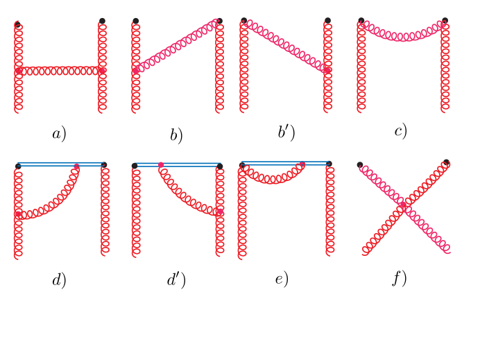
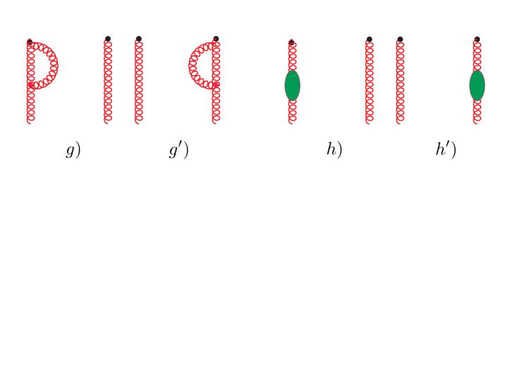
Figure 1: One-loop diagrams (mirror diagram $e^{\prime}$ is not shown).

3.1 Box diagram

For the “box” diagram shown in Fig. (1a), we have

$$\widetilde{F}_{(1a)} \left(x,p,q,\epsilon_{1},\epsilon_{2}\right)\Big{|}_{x\geq 0}={g^{2}C_{A}}\cdot 2i\varepsilon_{\alpha\mu\nu\rho}\bigg{[}({V_{011}^{\alpha}}-V_{101}^{\alpha}+V_{110}^{\alpha}-2q^{2}V_{111}^{\alpha})q^{\mu}\epsilon_{1}^{\nu}\epsilon_{2}^{*\rho}$$

$$+4p^{\mu}q^{\nu}\epsilon_{1}^{\rho}(-2T_{111}^{\alpha\beta}\epsilon_{2,\beta}^{*}+V_{111}^{\alpha}p\cdot\epsilon_{2}^{*})+4p^{\mu}q^{\nu}\epsilon_{2}^{*\rho}(2T_{111}^{\alpha\beta}\epsilon_{1,\beta}+V_{111}^{\alpha}q\cdot\epsilon_{1})\bigg{]}$$ (13)

Using explicit expressions for the basic integrals (see the Appendix) and simplifying, we obtain

$$\widetilde{F}_{(1a)} \left(x,p,q,\epsilon_{1},\epsilon_{2}\right)\Big{|}_{x\geq 0}=-\delta(x)\frac{g^{2}C_{A}}{8\pi^{2}{n\cdot P}}\left(\frac{\mu^{2}e^{\gamma_{E}}}{-q^{2}}\right)^{\epsilon}\frac{\Gamma^{2}(1-\epsilon)\Gamma(\epsilon)}{\Gamma(2-2\epsilon)}q^{2}\varepsilon(n,q,\epsilon_{1},\epsilon_{2}^{*})$$

$$-\delta^{\prime}(x)\frac{g^{2}C_{A}q^{2}}{16\pi^{2}{n\cdot P}}\left(\frac{\mu^{2}e^{\gamma_{E}}}{-q^{2}}\right)^{\epsilon}\frac{\Gamma^{2}(2-\epsilon)\Gamma(-1+\epsilon)}{\Gamma(4-2\epsilon)}\varepsilon(n,q,\epsilon_{1},\epsilon_{2}^{*})$$

$$+{\theta(0\leq x\leq 1)}\frac{g^{2}C_{A}}{8\pi^{2}{n\cdot P}}\bigg{[}2\,n\cdot p\,\varepsilon(p,q,\epsilon_{1},\epsilon_{2}^{*})\bigg{(}-\frac{4(1-x)^{1-2\epsilon}\Gamma(1-\epsilon)^{2}\Gamma(\epsilon)}{\Gamma(2-2\epsilon)}\left(\frac{\mu^{2}e^{\gamma_{E}}}{-q^{2}}\right)^{\epsilon}$$

$$+x\left(-\frac{1}{\epsilon}+\frac{1}{\epsilon_{\mathrm{IR}}}-\ln\frac{\mu^{2}}{\mu_{\mathrm{IR}}^{2}}+{\bigg{(}\frac{\mu_{\mathrm{IR}}^{2}e^{\gamma_{E}}}{-q^{2}}\bigg{)}^{\epsilon_{\mathrm{IR}}}}\frac{(1-x)^{-1-2\epsilon_{\mathrm{IR}}}\Gamma(-\epsilon_{\mathrm{IR}})^{2}\Gamma(1+\epsilon_{\mathrm{IR}})}{\Gamma(-2\epsilon_{\mathrm{IR}})}\right)\bigg{)}$$

$$+\frac{(1-x)^{-2\epsilon}\Gamma^{2}(1-\epsilon)\Gamma(\epsilon)}{\Gamma(2-2\epsilon)}\left(\frac{\mu^{2}e^{\gamma_{E}}}{-q^{2}}\right)^{\epsilon}\bigg{(}q^{2}(1-2\epsilon)\varepsilon(n,q,\epsilon_{1},\epsilon_{2}^{*})$$

$$+2\big{[}\varepsilon(n,p,q,\epsilon_{1})q\cdot\epsilon_{2}^{*}+\varepsilon(n,p,q,\epsilon_{2}^{*})q\cdot\epsilon_{1}\big{]}\Big{(}1-2x(1-\epsilon)\Big{)}\bigg{)}\bigg{]}\ .$$ (14)

Note that, in addition to the $\varepsilon(p,q,\epsilon_{1},\epsilon_{2})$ structure, there are other ones. Let us show that the other structures can be reduced to $\varepsilon(p,q,\epsilon_{1},\epsilon_{2})$. Indeed, if the vectors $p,q,\epsilon_{1},\epsilon_{2}$ are linearly independent in the $d=4$ space-time, the vector $n$ can be expressed in terms of the other 4 vectors as

$$n^{\mu}=a_{1}p^{\mu}+a_{2}(p+q)^{\mu}+a_{3}\epsilon_{1}^{\mu}+a_{4}\epsilon_{2}^{\mu}\ .$$ (15)

Contracting above equation with $p$, $p+q$ and $n$ respectively, we have

$$n\cdot p =-a_{2}\frac{q^{2}}{2}-a_{4}q\cdot\epsilon_{2},$$ (16)

$$n\cdot p+n\cdot q =-a_{1}\frac{q^{2}}{2}+a_{3}q\cdot\epsilon_{1},$$ (17)

$$0 =a_{1}n\cdot p+a_{2}(n\cdot p+n\cdot q).$$ (18)

In the zero-skewness case, we have $n\cdot q=0$, hence $a_{1}+a_{2}=0$ and also

$$\varepsilon(n,p,q,\epsilon_{1})q\cdot\epsilon_{2}^{*}+\varepsilon(n,p,q,\epsilon_{2}^{*})q\cdot\epsilon_{1}=2\,n\cdot p\,\varepsilon(p,q,\epsilon_{1},\epsilon_{2}^{*})$$ (19)

Similarly, for the $\varepsilon(n,q,\epsilon_{1},\epsilon_{2}^{*})$ structure, we have

$$\varepsilon(n,q,\epsilon_{1},\epsilon_{2}^{*})=(a_{1}+a_{2})\varepsilon(p,q,\epsilon_{1},\epsilon_{2}^{*})=0$$ (20)

As a result, the terms proportional to $\delta(x)$ and $\delta^{\prime}(x)$ vanish, and the remaining terms may be written as

$$\widetilde{F}_{(1a)} \left(x,p,q,\epsilon_{1},\epsilon_{2}\right)\Big{|}_{x\geq 0}={\theta(0\leq x\leq 1)}\frac{g^{2}C_{A}}{4\pi^{2}}\varepsilon(p,q,\epsilon_{1},\epsilon_{2}^{*})$$

$$\times\bigg{[}x\left(-\frac{1}{\epsilon}+\frac{1}{\epsilon_{\mathrm{IR}}}-\ln\frac{\mu^{2}}{\mu_{\mathrm{IR}}^{2}}+\left(\frac{\mu_{\mathrm{IR}}^{2}e^{\gamma_{E}}}{-q^{2}}\right)^{\epsilon_{\mathrm{IR}}}\frac{(1-x)^{-1-2\epsilon_{\mathrm{IR}}}\Gamma^{2}(-\epsilon_{\mathrm{IR}})\Gamma(1+\epsilon_{\mathrm{IR}})}{\Gamma(-2\epsilon_{\mathrm{IR}})}\right)$$

$$-\frac{2(1-x)^{-2\epsilon}\Gamma^{2}(1-\epsilon)\Gamma(\epsilon)}{\Gamma(2-2\epsilon)}\left(\frac{\mu^{2}e^{\gamma_{E}}}{-q^{2}}\right)^{\epsilon}(1-2x\epsilon)\bigg{]}.$$ (21)

Thus, the box diagram has both ultraviolet (UV) and infrared (IR) singular contributions, reflected by the UV poles $1/\epsilon$ and IR poles $1/\epsilon_{\mathrm{IR}}$.

3.2 Bremsstrahlung diagrams

For the diagram (1d), containing an insertion into the gluon link, we have

$${g^{2}C_{A}}\frac{2i}{n\cdot P(1-x)}\varepsilon_{\alpha\mu\nu\rho}(p+q)^{\mu}\epsilon_{2}^{*\rho}\bigg{[}n\cdot P(1+x)\epsilon_{1}^{\nu}V_{110}^{\alpha}-2n^{\nu}\epsilon_{1\beta}T_{110}^{\alpha\beta}\bigg{]}$$

$$= -\frac{\alpha_{s}C_{A}}{2\pi}\varepsilon(p,q,\epsilon_{1},\epsilon_{2}^{*})\left(\frac{1}{\epsilon}-\frac{1}{\epsilon_{\mathrm{IR}}}+\ln\frac{\mu^{2}}{\mu_{\mathrm{IR}}^{2}}\right)\bigg{[}\frac{x(1+x)}{1-x}{\theta(0\leq x\leq 1)}\bigg{]}_{+}\ .$$ (22)

For the mirror diagram (${\rm 1d}^{\prime}$), we obtain

$$-{g^{2}C_{A}}\frac{2i}{n\cdot P(1-x)}\varepsilon_{\alpha\mu\nu\rho}p^{\mu}\epsilon_{1}^{\nu}\bigg{[}n\cdot P(1+x)\epsilon_{2}^{*\rho}\left(V_{011}^{\alpha}+q^{\alpha}S_{011}\right)$$

$$-2n^{\rho}\left(\epsilon_{2,\beta}^{*}\left(T_{011}^{\alpha\beta}+q^{\alpha}V_{011}^{\beta}\right)-p\cdot\epsilon_{2}^{*}\left(V_{011}^{\alpha}+q^{\alpha}S_{011}\right)\right)\bigg{]}$$

$$= -\frac{\alpha_{s}C_{A}}{2\pi}\varepsilon(p,q,\epsilon_{1},\epsilon_{2}^{*})\left(\frac{1}{\epsilon}-\frac{1}{\epsilon_{\mathrm{IR}}}+\ln\frac{\mu^{2}}{\mu_{\mathrm{IR}}^{2}}\right)\bigg{[}\frac{x(1+x)}{1-x}{\theta(0\leq x\leq 1)}\bigg{]}_{+}\ .$$ (23)

Thus, the final expressions for contributions of diagrams (1d) and (${\rm 1d}^{\prime}$) coincide, and their combined contribution is given by

$$\widetilde{F}_{(1d)+(1d^{\prime})}\left(x,p,q,\epsilon_{1},\epsilon_{2}\right)\Big{|}_{x\geq 0}= -\frac{\alpha_{s}C_{A}}{\pi}\varepsilon(p,q,\epsilon_{1},\epsilon_{2}^{*})\left(\frac{1}{\epsilon}-\frac{1}{\epsilon_{\mathrm{IR}}}+\ln\frac{\mu^{2}}{\mu_{\mathrm{IR}}^{2}}\right)$$

$$\times\bigg{[}\frac{x(1+x)}{1-x}{\theta(0\leq x\leq 1)}\bigg{]}_{+}\ .$$ (24)

Note, that these diagrams contain the $\sim 1/(1-x)$ “bremsstrahlung” or soft-gluon exchange term. The singularity for $x=1$ comes here regularized by the “plus” prescription. In fact, the diagram (1a) also has the $\sim 1/(1-x)$ contribution, but it is not accompanied by the “plus” prescription. Namely, it comes from the term containing $(1-x)^{-1-2\epsilon_{\mathrm{IR}}}$.

To combine the contributions of the diagrams (1a), (1d) and (${\rm 1d}^{\prime}$), we write the expression for the diagram (1a) as a sum of a term having the plus-prescription for $x=1$ and a $\delta(1-x)$ term. Expanding in $\epsilon$, ${\epsilon_{\mathrm{IR}}}$, and neglecting the terms vanishing when $\epsilon=0$, ${\epsilon_{\mathrm{IR}}}=0$, we obtain

$$\widetilde{F}_{(1a)} \left(x,p,q,\epsilon_{1},\epsilon_{2}\right)\Big{|}_{x\geq 0}=\frac{\alpha_{s}}{\pi}C_{A}\epsilon(p,q,\epsilon_{1},\epsilon_{2}^{*})\bigg{\{}{\theta(0\leq x\leq 1)}$$

$$\times \bigg{[}-\frac{2+x}{\epsilon}+\frac{x(1+x)}{1-x}\left(-\frac{1}{\epsilon_{\mathrm{IR}}}+\ln\frac{\mu^{2}}{\mu_{\mathrm{IR}}^{2}}\right)-\frac{2}{1-x}\ln\frac{\mu^{2}}{-q^{2}(1-x)^{2}}-4(1-x)\bigg{]}\bigg{\}}_{+}$$

$$+\frac{\alpha_{s}}{\pi}C_{A}\epsilon(p,q,\epsilon_{1},\epsilon_{2}^{*})\delta(1-x)$$

$$\times\bigg{[}\frac{1}{\epsilon_{\mathrm{IR}}^{2}}+\frac{1}{\epsilon_{\mathrm{IR}}}\ln\frac{\mu_{\mathrm{IR}}^{2}}{-q^{2}}+\frac{1}{2}\ln^{2}\frac{\mu_{\mathrm{IR}}^{2}}{-q^{2}}-\frac{\pi^{2}}{12}-2-\frac{5}{2}\bigg{(}\frac{1}{\epsilon}-\frac{1}{\epsilon_{\mathrm{IR}}}+\ln\frac{\mu^{2}}{\mu_{\mathrm{IR}}^{2}}\bigg{)}\bigg{]}\,.$$ (25)

Note that the combination proportional to the IR factor $\left(-\frac{1}{\epsilon_{\mathrm{IR}}}+\ln\frac{\mu^{2}}{\mu_{\mathrm{IR}}^{2}}\right)$ in the second line of Eq. (25) cancels the IR part of the bremsstrahlung contribution (24).

3.3 Other vertex diagrams

The remaining vertex diagrams (1b), ($1{\rm b}^{\prime}$) , (1c), (${\rm 1e}$), (${\rm 1e}^{\prime}$) and (1f) vanish in Feynman gauge. In particular, for the diagram shown in Fig. (1b), we have

$${g^{2}C_{A}\cdot}6i\varepsilon_{\alpha\mu\nu\rho}V_{110}^{\alpha}p^{\mu}\epsilon_{1}^{\nu}\epsilon_{2}^{*\rho}=0\ ,$$ (26)

since $V_{110}^{\alpha}\sim p^{\alpha}$ according to Eq. (49). For the diagram ($1{\rm b}^{\prime}$), the result is

$${g^{2}C_{A}\cdot}6i\varepsilon_{\alpha\mu\nu\rho}\epsilon_{1}^{\nu}\epsilon_{2}^{*\rho}(p^{\mu}V_{011}^{\alpha}+q^{\mu}V_{011}^{\alpha}-p^{\alpha}q^{\mu}S_{011})\ .$$ (27)

It also vanishes after we use $V_{011}^{\alpha}=-((1-x)q^{\alpha}-xp^{\alpha})S_{011}$ (see Eqs. (47), (50)). For the diagram (1c), the result is identically zero. The contributions of the diagrams (${\rm 1e}$)

$${g^{2}C_{A}}\frac{2i}{n\cdot P(1-x)}\varepsilon_{\alpha\beta\mu\nu}n^{\alpha}p^{\beta}\epsilon_{1}^{\mu}\epsilon_{2}^{*\nu}S_{010}$$ (28)

and (${\rm 1e}^{\prime}$)

$${g^{2}C_{A}}\frac{2i}{n\cdot P(1-x)}\varepsilon_{\alpha\beta\mu\nu}n^{\alpha}(p+q)^{\beta}\epsilon_{1}^{\mu}\epsilon_{2}^{*\nu}S_{010}$$ (29)

are proportional to the function

$$S_{010}=\int\frac{\differential^{d}k}{(2\pi)^{d}k^{2}}\delta\left(x-1-\frac{n\cdot k}{n\cdot P}\right)\ .$$ (30)

Substituting the integrand factor by

$$\frac{1}{k^{2}}\delta\left(x-1-\frac{n\cdot k}{n\cdot P}\right)=\frac{1}{2\pi i}\int_{-\infty}^{\infty}\differential\gamma\,e^{i\gamma(x-1-{n\cdot k}/{n\cdot P})}\int_{0}^{\infty}\differential\alpha e^{i\alpha k^{2}}\ ,$$ (31)

and using the fact that the resulting Gaussian $k$-integral does not depend on $n$ when $n^{2}=0$,

$$\int\differential^{d}ke^{i\alpha k^{2}-i\gamma{n\cdot k}/{n\cdot P}}=\int\differential^{d}ke^{i\alpha k^{2}}\ ,$$ (32)

we see that $S_{010}$ reduces to

$$S_{010}=\delta(x-1)\int\frac{\differential^{d}k}{(2\pi)^{d}k^{2}}\ ,$$ (33)

i.e., to the integral containing just one propagator. Such integrals are treated as zero in the dimensional regularization.

Finally, the contributions of the four-gluon vertex diagram (1f) is identically zero.

3.4 Self-energy-type diagrams

We should also include the contributions of the diagrams of self-energy type. They have both UV and IR logarithmic divergences. We will present here the results for $x>0$, understanding that one should complement them by the $\{x\to-x\}$ contributions in the final result. In particular, the diagram (1g) is given by

$$-i\delta(1-x)\varepsilon(p,q,\epsilon_{1},\epsilon_{2}^{*})g^{2}C_{A}\int\frac{\differential^{d}k}{(2\pi)^{d}}\frac{3}{k^{2}(p-k)^{2}}$$ (34)

which produces

$$\delta(1-x)\varepsilon(p,q,\epsilon_{1},\epsilon_{2}^{*})\frac{\alpha_{s}C_{A}}{\pi}\frac{3}{4}\left(\frac{1}{\epsilon}-\frac{1}{\epsilon_{\mathrm{IR}}}+\ln\frac{\mu^{2}}{\mu_{\mathrm{IR}}^{2}}\right)$$ (35)

in the $\overline{\mbox{{\rm MS}}}\$scheme. Its mirror-conjugate diagram $({\rm 1g}^{\prime})$ gives the same contribution

$$\delta(1-x)\varepsilon(p,q,\epsilon_{1},\epsilon_{2}^{*})\frac{\alpha_{s}C_{A}}{\pi}\frac{3}{4}\left(\frac{1}{\epsilon}-\frac{1}{\epsilon_{\mathrm{IR}}}+\ln\frac{\mu^{2}}{\mu_{\mathrm{IR}}^{2}}\right)\ .$$ (36)

The self-energy corrections (${\rm 1h}$), (${\rm 1h}^{\prime}$) to the external gluon lines produce

$$Z_{g}\tilde{F}^{(0)}(x)=-2\varepsilon(p,q,\epsilon_{1},\epsilon_{2}^{*})\delta(1-x)\frac{\alpha_{s}}{\pi}\left(\frac{5}{12}C_{A}-\frac{1}{3}T_{F}n_{f}\right)\left(\frac{1}{\epsilon}-\frac{1}{\epsilon_{\mathrm{IR}}}+\ln\frac{\mu^{2}}{\mu_{\mathrm{IR}}^{2}}\right)\ .$$ (37)

4 One-loop corrections in light-cone gauge

To verify gauge invariance of our results presented in the previous section, we also perform a calculation in the light-cone gauge. The well-known advantage of the light-cone gauge is the absence of the gauge link. As a result, the diagrams 1(b), 1(b^′), 1(e), 1(e^′) are automatically zero, and “everything” comes from the box diagram  1(a), for which we have obtained

$$\widetilde{F}_{(1a)}(x,p,q,\epsilon_{1},\epsilon_{2})\bigg{|}_{x\geq 0}$$

$$=g^{2}C_{A}\cdot 2i\varepsilon_{\alpha\mu\nu\rho}\bigg{[}\bigg{(}\frac{2}{1-x}V_{011}^{\alpha}+\frac{2}{1-x}V_{110}^{\alpha}-2q^{2}V_{111}^{\alpha}-V_{101}^{\alpha}\bigg{)}q^{\mu}\epsilon_{1}^{\nu}\epsilon_{2}^{*\rho}$$

$$+\frac{2}{x}\frac{1}{n\cdot P}V_{101}^{\alpha}n^{\mu}q^{\nu}\epsilon_{2}^{*\rho}q\cdot\epsilon_{1}-\left(\frac{1}{x}V_{101}^{\alpha}+\frac{2}{1-x}V_{011}^{\alpha}\right)\frac{1}{n\cdot P}n^{\mu}q^{\nu}\epsilon_{1}^{\rho}q\cdot\epsilon_{2}^{*}$$

$$+4V_{111}^{\alpha}p^{\mu}q^{\nu}\left(\epsilon_{2}^{*\rho}q\cdot\epsilon_{1}-\epsilon_{1}^{\rho}q\cdot\epsilon_{2}^{*}\right)$$

$$+\frac{2}{1-x}\frac{1}{n\cdot P}n^{\mu}q^{\nu}\left(T_{110}^{\alpha\beta}\epsilon_{2}^{*\rho}\epsilon_{1,\beta}-T_{011}^{\alpha\beta}\epsilon_{1}^{\rho}\epsilon_{2,\beta}^{*}\right)-\frac{3}{x}\frac{1}{n\cdot P}T_{101}^{\alpha\beta}n^{\mu}q^{\nu}\left(\epsilon_{1}^{\rho}\epsilon_{2,\beta}^{*}-\epsilon_{2}^{*\rho}\epsilon_{1,\beta}\right)$$

$$+8T_{111}^{\alpha\beta}p^{\mu}q^{\nu}\left(\epsilon_{2}^{*\rho}\epsilon_{1\beta}-\epsilon_{1}^{\rho}\epsilon_{2,\beta}^{*}\right)\bigg{]}\,.$$ (38)

Using the expressions for the integrals given in the Appendix, we get

$$\delta(x)\frac{g^{2}C_{A}q^{2}}{96\pi^{2}n\cdot Px(1-x)}\varepsilon(n,q,\epsilon_{1},\epsilon_{2}^{*})\bigg{[}(6-17x(1-x))\left(\frac{1}{\epsilon}+\ln\frac{\mu^{2}}{-q^{2}}\right)+\frac{16\left(3-7x(1-x)\right)}{3}\bigg{]}$$

$$+\delta^{\prime}(x)\frac{g^{2}C_{A}q^{2}}{96\pi^{2}n\cdot P(1-x)}\varepsilon(n,q,\epsilon_{1},\epsilon_{2}^{*})\bigg{(}\frac{1}{\epsilon}+\ln\frac{\mu^{2}}{-q^{2}}+\frac{8}{3}\bigg{)}$$

$$+\theta(0\leq x<1)\bigg{[}-\frac{g^{2}C_{A}}{2\pi^{2}}\varepsilon(p,q,\epsilon_{1},\epsilon_{2}^{*})\left(\frac{2-3x+2x^{2}}{1-x}\left(\frac{1}{\epsilon}+\ln\frac{\mu^{2}}{-q^{2}(1-x)^{2}}\right)+4(1-x)\right)$$

$$+\frac{g^{2}C_{A}q^{2}}{8\pi^{2}n\cdot P}\varepsilon(n,q,\epsilon_{1},\epsilon_{2}^{*})\left(\frac{1}{\epsilon}+\ln\frac{\mu^{2}}{-q^{2}(1-x)^{2}}\right)$$

$$+\frac{g^{2}C_{A}}{4\pi^{2}n\cdot P}\left(\varepsilon(n,p,q,\epsilon_{1})q\cdot\epsilon_{2}^{*}+\varepsilon(n,p,q,\epsilon_{2}^{*})q\cdot\epsilon_{1}\right)$$

$$\times\left((1-2x)\left(\frac{1}{\epsilon}+\ln\frac{\mu^{2}}{-q^{2}(1-x)^{2}}\right)+2(1-x)\right)\bigg{]}\,,$$ (39)

where we have expanded the results in $\epsilon$. Now, recalling Eqs. (19) and (20), we find that only the structure $\varepsilon(p,q,\epsilon_{1},\epsilon_{2}^{*})$ is left, and we have

$$\widetilde{F}_{(1a)}(x,p,q,\epsilon_{1},\epsilon_{2})\bigg{|}_{x\geq 0}$$

$$= \frac{\alpha_{s}C_{A}}{\pi}\Pi(p,q,\epsilon_{1},\epsilon_{2}^{*})\theta(0\leq x<1)\bigg{[}\frac{1}{1-x}\bigg{(}\frac{1}{\epsilon}+\ln\frac{\mu^{2}}{-q^{2}(1-x)^{2}}\bigg{)}+2(1-x)\bigg{]}+\{x\to-x\}\,,$$ (40)

where the $-1<x\leq 0$ part is also included. One can observe that this expression is the same as the $x\neq\pm 1$ part of the total result obtained in Feynman gauge.

There are four other diagrams 1(b), 1(b^′), 1(c), 1(f), which, in principle, could contribute corrections for $x\neq\pm 1$ in the light-cone gauge. However, they produce no such contributions. To begin with, one can find that 1(c) is zero by contracting the indices. For Fig. 1(b), we have

$$g^{2}C_{A}\bigg{(}\frac{1}{x}V_{001}^{\alpha}+\frac{1}{1-x}V_{010}^{\alpha}\bigg{)}\frac{2i}{n\cdot P}\varepsilon_{\alpha\mu\nu\rho}n^{\mu}\epsilon_{1}^{\nu}\epsilon_{2}^{*\rho}\,,$$ (41)

and for Fig. 1(b^′) we obtain

$$g^{2}C_{A}\left(\frac{1}{1-x}V_{010}^{\alpha}+\frac{1}{x}V_{100}^{\alpha}\right)\frac{2i}{n\cdot P}\varepsilon_{\alpha\mu\nu\rho}n^{\mu}\epsilon_{1}^{\nu}\epsilon_{2}^{*\rho}\ .$$ (42)

For Fig. 1(f), we have

$$-g^{2}C_{A}\frac{1}{2x}V_{101}^{\alpha}n^{\mu}q^{\nu}(\epsilon_{1}^{\rho}q\cdot\epsilon_{2}^{*}+\epsilon_{2}^{*\rho}q\cdot\epsilon_{1})\frac{2i}{n\cdot P}\varepsilon_{\alpha\mu\nu\rho}\,.$$ (43)

According to the integrals listed in the Appendix, the contributions from the diagrams 1(b), 1(b^′) and 1(f) are all zero. Hence, the only nonzero correction for $x\neq\pm 1$ is from the box diagram Fig. 1(a), and we get the same result for $x\neq\pm 1$ in both Feynman and light-cone gauges.

The calculation of the $\sim\delta(1\pm x)$ contributions produced in the light-cone gauge by self-energy-type diagrams is a well-known routine, and we skip it. Some of such contributions combine with the $x\neq\pm 1$ terms into the “plus-prescription” expressions, and the others generate anomalous dimensions of the local operator.

5 Total result

Combining the contributions from all diagrams, we get the total result, which, including the tree-level contribution, reads

$$F(x,q^{2};\mu^{2},\mu_{\mathrm{IR}}^{2})= \Pi(p,q,\epsilon_{1},\epsilon_{2}^{*})$$

$$\times\Bigg{\{}1+\frac{\alpha_{s}}{\pi}C_{A}\bigg{\{}{\theta(0\leq x\leq 1)}\bigg{[}\frac{1}{1-x}\bigg{(}\frac{1}{\epsilon}+\ln\frac{\mu^{2}}{-q^{2}(1-x)^{2}}\bigg{)}+2(1-x)\bigg{]}\bigg{\}}_{+}$$

$$\hskip 28.45274pt+\frac{\alpha_{s}}{4\pi}\beta_{0}\delta(1-x)\left(\frac{1}{\epsilon}-\frac{1}{\epsilon_{\mathrm{IR}}}+\ln\frac{\mu^{2}}{\mu_{\mathrm{IR}}^{2}}\right)$$

$$\hskip 28.45274pt-\frac{\alpha_{s}}{\pi}C_{A}\delta(1-x)\bigg{(}\frac{1}{2\epsilon_{\mathrm{IR}}^{2}}+\frac{1}{2\epsilon_{\mathrm{IR}}}\ln\frac{\mu_{\mathrm{IR}}^{2}}{-q^{2}}+\frac{1}{4}\ln^{2}\frac{\mu_{\mathrm{IR}}^{2}}{-q^{2}}-\frac{\pi^{2}}{24}-1\bigg{)}\Bigg{\}}$$

$$\hskip 28.45274pt+\{x\to-x\}\ .$$ (44)

The coefficient accompanying the $1/\epsilon$ pole (multiplied by the $\alpha_{s}/2\pi$ factor) gives the evolution kernel

$$P_{gg}^{\widetilde{F}}(x)=\frac{\beta_{0}}{2}\delta(1-x)+C_{A}\bigg{[}\frac{2}{1-x}\theta(0\leq x\leq 1)\bigg{]}_{+}+\{x\to-x\}\$$ (45)

for $\widetilde{F}(x,q^{2})$. It has two ingredients. The $\sim\beta_{0}$ term corresponds to the anomalous dimension of the local operator $F^{\mu\nu}(0)\widetilde{F}_{\mu\nu}(0)$. The “plus-prescription” term, displayed in the second line of Eq. (44), is specific for the nonlocal case. Note that it does not contain the IR poles ${\epsilon_{\mathrm{IR}}}$ and the IR scale $\mu_{\mathrm{IR}}$. As already mentioned, the terms $\sim\left(-{1}/{\epsilon_{\mathrm{IR}}}+\ln{\mu^{2}}/{\mu_{\mathrm{IR}}^{2}}\right)$ present in the box and bremsstrahlung diagrams, cancel each other. As a result, the IR cutoff in this term is provided by the momentum transfer $q^{2}$, just like in the case of the “gluon condensate” PDF $F(x)$ discussed in our recent paper Radyushkin:2021fel (a similar observation was made in the studies of the quark GPDs Liu:2019urm , Ji:2015qla ).

Another observation is that the kernel $P_{gg}^{\widetilde{F}}(x)$ coincides with that for the “gluon condensate” PDF $F(x)$, despite the difference in the structure of the relevant nonlocal operators. However, our expression for the evolution kernel does not coincide with that obtained in Ref. Hatta:2020ltd .

The UV finite “Sudakov” term, shown in the $4{\rm th}$ line of Eq. (44), is an artifact of the IR regularization by a finite momentum transfer $q$. Recall that, to maintain the necessary strict gauge invariance in our calculations, we have chosen to take zero-virtuality initial and final momenta $p_{1},p_{2}$. Next, to get a non-vanishing result for the overall kinematical factor $\Pi(p,q,\epsilon_{1},\epsilon_{2}^{*})$ (see Eq. (5)), we have imposed a nonzero momentum transfer $q=p_{2}-p_{1}$, with $q^{2}\neq 0$. As a result, the box diagram (1a) is formally in the Sudakov kinematics $-q^{2}\gg|p_{1}^{2}|\sim|p_{2}^{2}|$, which is signalized by double logarithms in the Sudakov term. Because of its purely IR nature, we may absorb the “Sudakov” term into a “bare” GPD. In other words, since it does not contain the UV parameter $\mu$, the “Sudakov” term does not affect the relation between the functions $\widetilde{F}^{(1)}(x,q^{2};\mu^{2})$ at different evolution scales $\mu$. Similarly, calculating the matrix element $\langle p_{2}|F^{\mu\nu}\left(-{z}/{2}\right)W\left[-{z}/{2},{z}/{2}\right]\widetilde{F}_{\mu\nu}({z}/{2}|p_{1}\rangle$ for $z^{2}\neq 0$ (i.e., off the light cone, which is necessary for lattice calculations of $\widetilde{F}(x,q^{2};\mu^{2})$), one would get the same Sudakov terms, that would cancel in the matching condition between off-the-light-cone and on-the-light-cone versions of the GPD.

Finally, we would like to mention that we do not have $\delta(x)$ terms in our one-loop result (44) which one could identify as a “zero-mode” contribution.

6 Summary and outlook

In this paper, we have presented the results of one-loop corrections in the 2-gluon sector to the “topological charge” GPD $\widetilde{F}(x,q^{2})$ introduced in Ref. Hatta:2020ltd . Just like in our paper Radyushkin:2021fel about the “gluon condensate” PDF $F(x)$, to get a nonzero contribution for the gluon matrix element at the tree level and maintain gauge invariance, we took a nonforward matrix element between on-shell massless gluons, i.e. we have considered a GPD reducing to $\widetilde{F}(x)$ in the forward limit. Ref. Hatta:2020ltd also deals with a GPD, however, the calculation was done for off-shell gluons, which violates gauge invariance.

We have performed our calculations with on-shell external gluons both in Feynman and light-cone gauges, and obtained the same result. Our Feynman-gauge and light-cone-gauge calculations are described in the present paper on the diagram-by-diagram level. They give a result differing from that of Ref. Hatta:2020ltd , thus demonstrating once more the importance of doing the calculations of gluon matrix elements in a strict compliance with the gauge-invariance requirements.

In Ref. Ji:2020baz , it was suggested that some twist-4 gluon PDFs may have $\delta(x)$ zero-modes, similar to those observed in one-loop perturbative QCD expressions for the twist-3 quark PDFs (see, e.g., Burkardt:2001iy ). However, our one-loop expression for the twist-4 gluon GPD $\widetilde{F}(x,q^{2})$ does not contain such terms.

It should be emphasized that our calculation deals with the matrix elements of the twist-4 bilocal operator $F^{\mu\nu}\left(-{z}/{2}\right)\widetilde{F}_{\mu\nu}({z}/{2})$ (we skip the link factor $W$ here and below) between two external gluon states. In the OPE language, this means that we are picking out the $F^{\mu\nu}\left(uz\right)\widetilde{F}_{\mu\nu}(vz)$ terms in the expansion of the original operator product $F^{\mu\nu}\left(-\frac{z}{2}\right)\widetilde{F}_{\mu\nu}(\frac{z}{2})$. However, one can easily imagine twist-4 nonlocal operators built from three and even four gluon fields (like $z^{\alpha}z^{\beta}F_{\alpha\mu}\left(uz\right)F^{\mu\nu}(vz)\widetilde{F}_{\nu\beta}(wz)$, etc.). To pick out coefficient functions corresponding to such operators, one should consider matrix elements of $F^{\mu\nu}\left(-{z}/{2}\right)\widetilde{F}_{\mu\nu}({z}/{2})$ between three and four external gluons. In the momentum representation, such a procedure of calculating the mixing between different types of gluon operators involves some element of guessing and uncertainty about whether all possible combinations have been taken into account.

Another way to approach this problem is to calculate corrections in the operator form, without making projections on external states at all, like it was done in Refs. Radyushkin:2017lvu ; Balitsky:2019krf ; Balitsky:2021qsr ; Balitsky:2021cwr for the “twist-2” quark and gluon bilocal operators outside the light cone. This gives a possible direction for future studies of the twist-4 gluon distributions. A natural first step would be a coordinate-space formulation of the results obtained using the momentum-space techniques in the present paper and in Ref. Radyushkin:2021fel .

Appendix A Table of integrals

$$S_{010}\sim 0,$$ (46)

$$S_{011}= \frac{i}{16\pi^{2}}\bigg{(}\frac{1}{\epsilon}-\frac{1}{\epsilon_{\mathrm{IR}}}+\ln\frac{\mu^{2}}{\mu_{\mathrm{IR}}^{2}}\bigg{)}{\theta(0\leq x\leq 1)},$$ (47)

$$V_{100}^{\alpha}\sim V_{010}^{\alpha}\sim V_{001}^{\alpha}\sim 0,$$ (48)

$$V^{\mu}_{110}{\sim} \frac{i}{16\pi^{2}}\bigg{(}\frac{1}{\epsilon}-\frac{1}{\epsilon_{\mathrm{IR}}}+\ln\frac{\mu^{2}}{\mu_{\mathrm{IR}}^{2}}\bigg{)}xp^{\mu}{\theta(0\leq x\leq 1)},$$ (49)

$$V^{\mu}_{011}{\sim} -\frac{i}{16\pi^{2}}\left(\frac{1}{\epsilon}-\frac{1}{\epsilon_{\mathrm{IR}}}+\ln\frac{\mu^{2}}{\mu_{\mathrm{IR}}^{2}}\right)((1-x)q^{\mu}-xp^{\mu}){\theta(0\leq x\leq 1)},$$ (50)

$$V^{\mu}_{101}= -\frac{i}{16\pi^{2}}\left(\frac{\mu^{2}e^{\gamma_{E}}}{-q^{2}}\right)^{\epsilon}\Bigg{[}\Gamma(\epsilon)\frac{\Gamma(2-\epsilon)\Gamma(1-\epsilon)}{\Gamma(3-2\epsilon)}q^{\mu}\delta(x)+\frac{1}{2}\frac{q^{2}}{n\cdot P}\frac{\Gamma(2-\epsilon)^{2}}{\Gamma(4-2\epsilon)}\Gamma(-1+\epsilon)n^{\mu}\delta^{\prime}(x)\Bigg{]},$$ (51)

$$V^{\mu}_{111}= -\frac{i}{16\pi^{2}q^{2}}(\frac{\mu_{\mathrm{IR}}^{2}e^{\gamma_{E}}}{-q^{2}})^{\epsilon_{\mathrm{IR}}}\Gamma(1+\epsilon_{\mathrm{IR}})\frac{\Gamma(-\epsilon_{\mathrm{IR}})^{2}}{\Gamma(-2\epsilon_{\mathrm{IR}})}\bigg{[}\frac{1}{2}(1-x)^{-2\epsilon_{\mathrm{IR}}}q^{\mu}$$

$$-x(1-x)^{-1-2\epsilon_{\mathrm{IR}}}p^{\mu}\bigg{]}{\theta(0\leq x\leq 1)}$$

$$+\frac{i}{32\pi^{2}}\bigg{(}\frac{\mu^{2}e^{\gamma_{E}}}{-q^{2}}\bigg{)}^{\epsilon}\frac{\Gamma(1-\epsilon)^{2}\Gamma(\epsilon)}{\Gamma(2-2\epsilon)}\frac{n^{\mu}}{n\cdot P}\bigg{[}-\delta(x)$$

$$+(1-2\epsilon)(1-x)^{-2\epsilon}{\theta(0\leq x\leq 1)}\bigg{]},$$ (52)

$$T^{\mu\nu}_{110}\sim \frac{i}{16\pi^{2}}\bigg{(}\frac{1}{\epsilon}-\frac{1}{\epsilon_{\mathrm{IR}}}+\ln\frac{\mu^{2}}{\mu_{\mathrm{IR}}^{2}}\bigg{)}x^{2}p^{\mu}p^{\nu}{\theta(0\leq x\leq 1)},$$ (53)

$$T^{\mu\nu}_{011}\sim \frac{i}{16\pi^{2}}\bigg{(}\frac{1}{\epsilon}-\frac{1}{\epsilon_{\mathrm{IR}}}+\ln\frac{\mu^{2}}{\mu_{\mathrm{IR}}^{2}}\bigg{)}[(1-x)q^{\mu}-xp^{\mu}][(1-x)q^{\nu}-xp^{\nu}]{\theta(0\leq x\leq 1)},$$ (54)

$$T^{\mu\nu}_{101}\sim \frac{i}{16\pi^{2}}(\frac{\mu^{2}e^{\gamma_{E}}}{-q^{2}})^{\epsilon}\bigg{(}q^{2}\frac{g^{\mu\nu}}{2}\frac{\Gamma^{2}(2-\epsilon)}{\Gamma(4-2\epsilon)}\Gamma(-1+\epsilon)+\frac{\Gamma(3-\epsilon)\Gamma(1-\epsilon)}{\Gamma(4-2\epsilon)}\Gamma(\epsilon)q^{\mu}q^{\nu}\bigg{)}\delta(x)$$

$$+\frac{i}{16\pi^{2}}(\frac{\mu^{2}e^{\gamma_{E}}}{-q^{2}})^{\epsilon}\frac{q^{2}}{2}\frac{\Gamma^{2}(2-\epsilon)}{\Gamma(4-2\epsilon)}\Gamma(-1+\epsilon)\frac{q^{\mu}n^{\nu}+q^{\nu}n^{\mu}}{n\cdot P}\delta^{\prime}(x),$$ (55)

$$T^{\mu\nu}_{111}{\sim} \frac{i}{16\pi^{2}}\bigg{\{}\frac{g^{\mu\nu}}{2}(1-x)^{1-2\epsilon}\frac{\Gamma(1-\epsilon)^{2}}{\Gamma(2-2\epsilon)}\Gamma(\epsilon)(\frac{\mu^{2}e^{\gamma_{E}}}{-q^{2}})^{\epsilon}$$

$$+\frac{1}{q^{2}}\Gamma(1+\epsilon_{\mathrm{IR}})(\frac{\mu_{\mathrm{IR}}^{2}e^{\gamma_{E}}}{-q^{2}})^{\epsilon_{\mathrm{IR}}}\bigg{[}(1-x)^{1-2\epsilon_{\mathrm{IR}}}\frac{\Gamma(2-\epsilon_{\mathrm{IR}})\Gamma(-\epsilon_{\mathrm{IR}})}{\Gamma(2-2\epsilon_{\mathrm{IR}})}q^{\mu}q^{\nu}$$

$$-x(1-x)^{-2\epsilon_{\mathrm{IR}}}\frac{\Gamma(1-\epsilon_{\mathrm{IR}})\Gamma(-\epsilon_{\mathrm{IR}})}{\Gamma(1-2\epsilon_{\mathrm{IR}})}(q^{\mu}p^{\nu}+p^{\mu}q^{\nu})$$

$$+x^{2}(1-x)^{-1-2\epsilon_{\mathrm{IR}}}\frac{\Gamma(-\epsilon_{\mathrm{IR}})^{2}}{\Gamma(-2\epsilon_{\mathrm{IR}})}p^{\mu}p^{\nu}\bigg{]}\bigg{\}}{\theta(0\leq x\leq 1)}$$

$$-\frac{i}{32\pi^{2}n\cdot P}\bigg{(}\frac{\mu^{2}e^{\gamma_{E}}}{-q^{2}}\bigg{)}^{\epsilon}\Gamma(\epsilon)\frac{\Gamma^{2}(1-\epsilon)}{\Gamma(2-2\epsilon)}\bigg{\{}\bigg{[}-\frac{1}{2}\delta(x)$$

$$+(1-\epsilon)(1-x)^{1-2\epsilon}{\theta(0\leq x\leq 1)}\bigg{]}(n^{\mu}q^{\nu}+n^{\nu}q^{\mu})$$

$$+(1-x)^{-2\epsilon}(1-2(1-\epsilon)x)(n^{\mu}p^{\nu}+n^{\nu}p^{\mu}){\theta(0\leq x\leq 1)}\bigg{\}}.$$ (56)

Note: The sign $\sim$ means that, in addition to the explicitly written terms, the contribution also contains $\int\differential^{d}k/k^{2}$ terms which are treated as zero. The terms that vanish under contraction of indices are also neglected.

References

- (1) R. P. Feynman, Photon-hadron interactions. Reading, 1972.
- (2) Y. Hatta and Y. Zhao, Parton distribution function for the gluon condensate, Phys. Rev. D 102 (2020) 034004, [2006.02798].
- (3) Y. Hatta, -odd gluonic operators in QCD spin physics, Phys. Rev. D 102 (2020) 094004, [2009.03657].
- (4) X. Ji, Fundamental Properties of the Proton in Light-Front Zero Modes, Nucl. Phys. B (2020) 115181, [2003.04478].
- (5) M. Burkardt and Y. Koike, Violation of sum rules for twist three parton distributions in QCD, Nucl. Phys. B 632 (2002) 311–329, [hep-ph/0111343].
- (6) A. Radyushkin and S. Zhao, One-loop structure of parton distribution for the gluon condensate and “zero modes”, JHEP 12 (2021) 010, [2111.00887].
- (7) Y.-S. Liu, W. Wang, J. Xu, Q.-A. Zhang, J.-H. Zhang, S. Zhao et al., Matching generalized parton quasidistributions in the RI/MOM scheme, Phys. Rev. D 100 (2019) 034006, [1902.00307].
- (8) X. Ji, A. Schäfer, X. Xiong and J.-H. Zhang, One-Loop Matching for Generalized Parton Distributions, Phys. Rev. D 92 (2015) 014039, [1506.00248].
- (9) A. V. Radyushkin, Quark pseudodistributions at short distances, Phys. Lett. B 781 (2018) 433–442, [1710.08813].
- (10) I. Balitsky, W. Morris and A. Radyushkin, Gluon Pseudo-Distributions at Short Distances: Forward Case, Phys. Lett. B 808 (2020) 135621, [1910.13963].
- (11) I. Balitsky, W. Morris and A. Radyushkin, Short-distance structure of unpolarized gluon pseudodistributions, Phys. Rev. D 105 (2022) 014008, [2111.06797].
- (12) I. Balitsky, W. Morris and A. Radyushkin, Polarized Gluon Pseudodistributions at Short Distances, 2112.02011.