Eye Know You Too: A DenseNet Architecture for End-to-end Eye Movement Biometrics

Abstract

emb is a relatively recent behavioral biometric modality that may have the potential to become the primary authentication method in virtual- and augmented-reality devices due to their emerging use of eye-tracking sensors to enable foveated rendering techniques. However, existing eye movement biometrics (EMB) models have yet to demonstrate levels of performance that would be acceptable for real-world use. Deep learning approaches to EMB have largely employed plain convolutional neural networks, but there have been many milestone improvements to convolutional architectures over the years including residual networks and densely connected convolutional networks. The present study employs a DenseNet architecture for end-to-end EMB and compares the proposed model against the most relevant prior works. The proposed technique not only outperforms the previous state of the art, but is also the first to approach a level of authentication performance that would be acceptable for real-world use.

I Introduction

Biometrics have become a part of everyday life due to the ubiquity of fingerprint and face recognition in smartphones. Most biometric modalities can be separated into two categories: physical and behavioral. Physical biometrics reflect the physical traits of a person, including face, fingerprint, iris, and retina. Behavioral biometrics reflect a person’s patterns of behavior, with some of the most commonly studied modalities being gait, signature, and voice. Physical biometrics tend to be more distinctive and exhibit greater permanence, whereas behavioral biometrics tend to be less intrusive and more applicable for continuous authentication. An overview of these common biometric modalities is given in [1].

A more recent behavioral biometric modality is EMB [2]. Eye movements may be particularly spoof-resistant because the oculomotor system is controlled by a complex combination of neurological and physiological mechanisms, both voluntary and involuntary. Eye movements also enable liveness detection [3, 4] and continuous authentication [5, 6] and could easily be paired with other modalities like mouse dynamics [7] or iris recognition [8] in a multimodal biometrics system. Because eye movements have been shown to carry distinguishable information, studies have even begun to explore methods of deidentifying eye movement signals in an effort to preserve both the users’ privacy and the utility of the eye movements as an input method [9, 10, 11, 12, 13].

There is an emerging use of eye-tracking sensors in both virtual-reality (VR) and augmented-reality (AR) devices (e.g., Vive Pro Eye [14], Magic Leap 1 [15], HoloLens 2 [16]) in part to enable foveated rendering [17] techniques which offer a significant reduction in overall power consumption without a noticeable impact to visual quality. In addition to foveated rendering, eye tracking also enables various applications in these devices including user interactions, analytics, and various display technologies [18]. Because the hardware required for EMB is already included with these devices, and because EMB offers continuous authentication capabilities, EMB has the potential to become the primary security method for these devices [19]. However, existing EMB models have yet to demonstrate levels of authentication performance that would be acceptable for real-world use, even when using eye-tracking signals with higher levels of signal quality than are available in current VR/AR devices. Deep learning models for EMB [20, 21, 22, 4, 23] have largely been limited to plain convolutional neural networks (CNNs) which, despite being capable of outperforming more traditional statistical approaches, do not take advantage of milestone developments over the years in the area of convolutional architectures, including residual networks (ResNets) [24] and—the focus of the present study— densely connected convolutional networks (DenseNets) [25].

We propose a novel DenseNet-based architecture for end-to-end EMB. The model is trained and evaluated on the GazeBase [26] dataset which contains eye movement data from 322 subjects each recorded up to 18 times over a 37-month period. Although the eye-tracking signals in GazeBase reflect a higher level of signal quality than is available in current VR/AR devices, it is important to first establish whether EMB is capable, even with high-quality data, of achieving a level of authentication performance that is acceptable for real-world use. We primarily evaluate our model in the authentication scenario (also commonly called verification) using equal error rate (EER), both because authentication performance has been shown to remain relatively stable regardless of population size [27] and because behavioral biometric traits are generally not distinctive enough for large-scale identification [28]. We also perform additional analyses that we have seen only a small portion of works do (e.g., [23]), including assessing the permanence of the learned features and estimating the false rejection rate (FRR) at a false acceptance rate (FAR) of 1-in-10000 (abbreviated FRR @ FAR $10^{-4}$).

The main contributions of the present study are:

• A novel, highly parameter-efficient, DenseNet-based architecture that achieves state-of-the-art EMB performance in the authentication scenario on high-quality data, namely 3.66% EER when enrolling and authenticating with just 5 s of eye movements during a reading task. For perspective, 5 s is somewhat comparable to the time it takes to enter a 4-digit pin or to calibrate an eye-tracking device.

• The first to show that, using 30 s of eye movements during a reading task, it is possible to achieve an estimated 5% FRR @ FAR $10^{-4}$ which approaches a level of authentication performance that would be acceptable for real-world use.

• The first to report significantly better-than-chance FRR @ FAR $10^{-4}$ with 60 s of eye movements at artificially degraded sampling rates as low as 50 Hz, suggesting that EMB has the potential to become suitable for deployment at the sampling rates present in existing VR/AR devices.

• The first application of a more modern convolutional architecture for EMB.

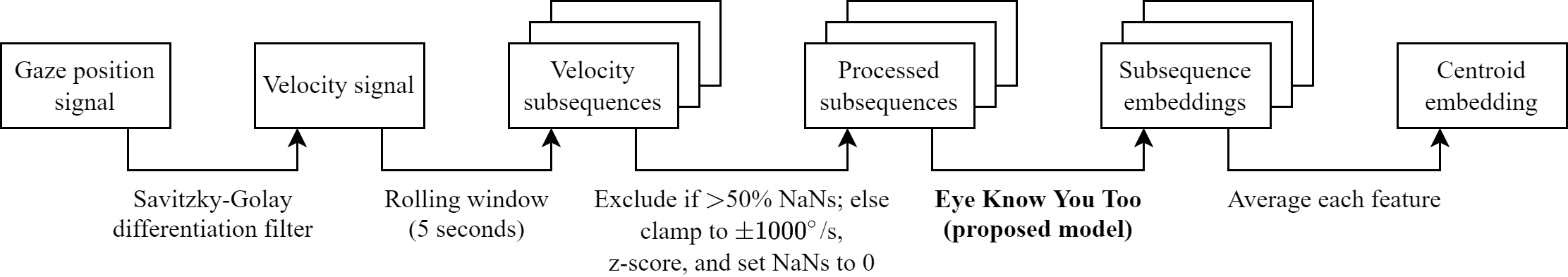
Figure 1: Overview of the process for embedding an eye-tracking signal using the proposed methodology. We primarily focus on the case where only the first 5-second window is embedded, but we explore aggregating embeddings across windows in § V-C.

II Prior Work

II-A cnn

Since the seminal works of AlexNet [29] and VGGNet [30], CNNs have quickly become some of the most popular types of neural networks for image processing tasks. Such architectures also started being employed in time series domains like eye movement event classification [31] and audio synthesis [32]. In time series domains such as these, varieties of recurrent neural networks (RNNs) [33, 34] were once the most common, but CNNs have empirically shown to be capable of similar-or-better performance while also being much faster to train [35].

Several pivotal architectural improvements have been made to CNNs since their infancy. We focus on two such improvements: ResNets [24] and DenseNets [25]. resnet [24] introduce so-called “skip connections” that combine the output of each convolutional block with its input via summation. These skip connections improve gradient flow through the network, enabling the training of significantly deeper networks than was previously possible. densenet [25] include similar skip connections between each convolutional block and all subsequent blocks, using channel-wise concatenation instead of summation to facilitate even better information flow than ResNets. One study visualizing loss landscapes [36] showed that DenseNets have much smoother loss landscapes than ResNets which may lead to increased ease of convergence during training.

We acknowledge that there are more recent convolutional architectures than DenseNet that claim better performance on image processing tasks (e.g., ResNeXT [37], DSNet [38], EfficientNet [39], EfficientNetV2 [40]), not to mention the various transformer [41, 42] architectures that have seen success in domains including natural language processing (NLP) and image classification. Rather than using one of these more cutting-edge architectures, we base our architecture on DenseNet because of its parameter efficiency and relative simplicity. We find that this architecture is able to achieve state-of-the-art performance in the EMB domain.

II-B emb

emb has been studied extensively since the introduction of the modality in 2004 [2]. Most earlier works in the field [43, 44, 45, 46, 47] require explicit classification of eye movement signals into physiologically-grounded events, from which hand-crafted features are extracted and fed into statistical or machine learning models. The state-of-the-art statistical model is the approach by Friedman et al. [45] which centers around the use of principal component analysis (PCA) and the intraclass correlation coefficient (ICC).

Since the recent introduction of deep learning to the field of EMB [20, 21], end-to-end deep learning approaches have become more common [20, 21, 22, 4, 23]. The current state-of-the-art model is DeepEyedentificationLive (DEL) [4] which utilizes two convolutional subnets that separately focus on “fast” (e.g., saccadic) and “slow” (e.g., fixational) eye movements. Another recent model, Eye Know You (EKY) [23], uses exponentially dilated convolutions to achieve reasonable biometric authentication performance with a relatively small ($\sim$475K learnable parameters) network architecture.

Both DEL and EKY employ plain CNN architectures that do not take advantage of the improvements made to CNNs over the years. The present study improves upon the previous state of the art by using a more modern DenseNet-based architecture to simultaneously increase expressive power and reduce parameter count.

III Network Architecture

The proposed network architecture, which we call Eye Know You Too (EKYT), is visualized in Fig. 2. The network performs a mapping $f:\mathbb{R}^{C\times T}\to\mathbb{R}^{128}$, where $C$ is the number of input channels, $T$ is the input sequence length, and the output is a 128-dimensional embedding. It begins with a single dense block of 8 one-dimensional convolution layers, where the feature maps produced by each convolution layer are concatenated with all previous feature maps before being fed into the next convolution layer. The final set of concatenated feature maps is then sent through a global average pooling layer, flattened, and then fed into a fully-connected layer to produce a 128-dimensional embedding of the input sequence. When classification is required (e.g., for cross-entropy loss), an additional fully-connected layer is appended after the embedding layer that outputs class logits.

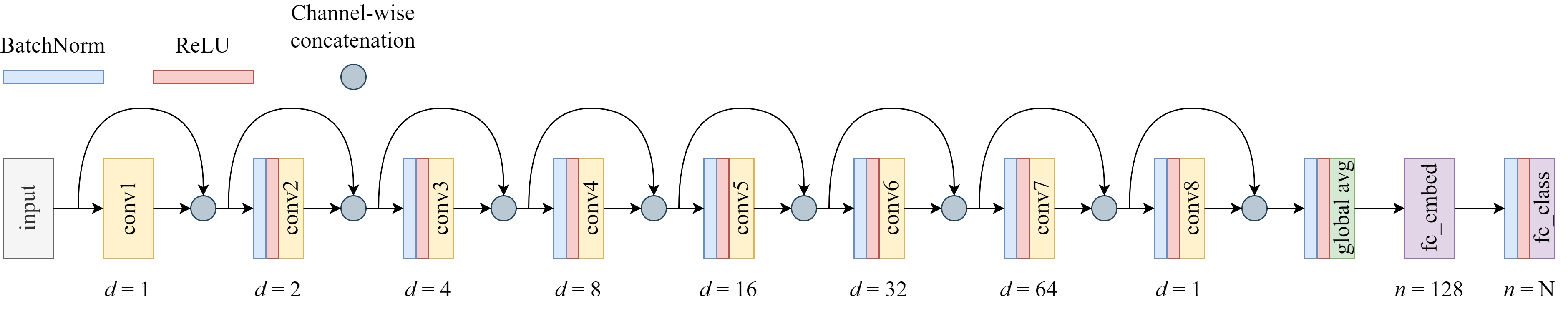
Figure 2: The proposed pre-activation DenseNet-based network architecture, including the optional classification layer. Each convolution layer has kernel size $k=3$, stride $s=1$, and dilation rate $d$ that varies by layer. Each convolution layer outputs 32 feature maps that are concatenated with the previous feature maps before being fed into the next convolution layer.

All convolution layers (except the first), the global average pooling layer, and the optional classification layer are all preceded by batch normalization (BN) [48] and the rectified linear unit (ReLU) [49] activation function (called a “pre-activation” architecture). We use a “growth rate” of 32, meaning each convolution layer outputs 32 feature maps to be concatenated with the previous feature maps. Because we use BN, there is no need for the convolution layers to learn an additive bias.

The convolution layers (labeled $n=1,\dotsc,8$) use constant kernel size $k=3$ and stride $s=1$, an exponentially increasing dilation rate $d_{n}=2^{(n-1)\bmod 7}$, and enough zero padding $p_{n}=d_{n}$ on both sides of the input to preserve the length along the feature dimension. The use of exponentially dilated convolutions produces an exponential growth of the receptive field of the network with only a linear increase in the number of learnable parameters. In general, assuming $s=1$, the receptive field of layer $n$, denoted $r_{n}$, is given by

$$r_{n}=1+\sum_{i=1}^{n}{d_{n}(k_{n}-1)}.$$ (1)

The final convolution layer of our network has a (maximum) receptive field of $r_{8}=257$ time steps from the input.

Excluding the optional classification layer, our proposed architecture has $\sim$123K learnable parameters for $C=2$ and any $T$. Weights are initialized in the following manner. Each convolutional layer uses He initialization [50] with a normal distribution and learns no additive bias. Each BN layer is initialized with a weight of 1 and a bias of 0. Each fully-connected layer is initialized with a bias of 0, and weights are initialized using the default method of PyTorch 1.10.0.

In preliminary experiments, we experienced overfitting on the train set relative to the validation set when increasing the depth of the network and/or adding additional dense blocks (each separated by a transition block to optionally reduce the size of the channel dimension). Specialized dropout techniques have been proposed for DenseNet architectures to resolve such overfitting problems [51]; but in the interest of keeping our network small, we did not pursue such techniques. We also experienced worse performance when using global max pooling instead of global average pooling. We found no noticeable difference in performance when swapping the order of BN and ReLU, nor when using a “post-activation” architecture (i.e., applying BN and ReLU after each convolution before channel-wise concatenation). Though, we note that pre-activation DenseNet (and ResNet) architectures generally produce lower errors than their post-activation counterparts [52].

IV Methodology

IV-A Hardware & software

All models are trained inside Docker containers on a Lambda Labs workstation. The workstation is equipped with quad NVIDIA GeForce RTX A5000 GPUs (24 GB VRAM), an AMD Ryzen Threadripper PRO 3975WX CPU @ 3.5 GHz (32 cores), and 256 GB RAM. Each Docker container runs Ubuntu 18.04 with the most notable packages being Python 3.7.11, PyTorch [53] 1.10.0, and PyTorch Metric Learning (PML) [54] 0.9.99. PyTorch Lightning [55] 1.5.0 is used to accelerate development. Experiments are logged using Weights & Biases [56] 0.12.1. For visualizing the embedding space, we employ umap-learn [57] 0.5.1.

Our full source code and trained models are available on the Texas State Digital Collections Repository at [TO BE PUBLISHED AFTER ACCEPTANCE].

IV-B Dataset

We use the GazeBase [26] dataset consisting of 322 college-aged participants, each recorded monocularly (left eye only) at 1000 Hz using an EyeLink 1000 eye tracker. Nine rounds of recordings (R1–9) were captured over a period of 37 months. Each subsequent round comprises a subset of participants from the preceding round (with one exception, participant 76, who was not present in R3 but returned for R4–5), with only 14 of the initial 322 participants present across all 9 rounds. Each round consists of 2 recording sessions separated by approximately 30 minutes. During each recording session, participants performed a battery of 7 tasks: random saccades (RAN), horizontal saccades (HSS), fixation (FXS), an interactive ball-popping game (BLG), reading (TEX), and two video-viewing tasks (VD1 and VD2). More details about each task can be found in the dataset’s paper [26].

We create class-disjoint train and test sets by assigning the 59 participants present during R6 to the test set and the remaining 263 participants to the train set. In this way, the test set—which comprises nearly 50% of all recordings in GazeBase—can be used to assess the generalizability of our model both to out-of-sample participants and to longer test-retest intervals than are present during training. The train set is further partitioned into 4 class-disjoint folds in a way that balances the number of participants and recordings between folds as well as possible (the fold assignment algorithm we use is described in [23]). These 4 folds are used for 4-fold cross-validation, where 1 fold acts as the validation set and the remaining folds act as the train set. We exclude the BLG task from the train and validation sets due to the large variability in its duration relative to the other tasks, but we include it in the test set to enable an assessment of our model on an out-of-sample task.

We used 4-fold cross-validation to manually tweak our network architecture and determine the final training parameters. Only at the very end of our experiments did we use the test set to get a final, unbiased estimate of our model’s performance.

IV-C Data preprocessing

We start with a sequence of $T_{\text{record}}$ tuples $\left(t^{(i)},\,x^{(i)},\,y^{(i)}\right)$, $i=1,\dotsc,T_{\text{record}}$, where $t^{(i)}$ is the time stamp (s) and $x^{(i)}$, $y^{(i)}$ are the horizontal and vertical components of the monocular (left eye) gaze position (^∘). Next, we estimate the first derivative (i.e., velocity in ^∘/s) of the horizontal and vertical channels using a Savitzky-Golay [58] differentiation filter with order 2 and window size 7, inspired by [45].

Each recording is then split into non-overlapping windows of 5 s ($T=5000$ time steps) using a rolling window. Excess time steps at the end of a recording that would form only a partial window are discarded. Although previous studies like DEL [4] and EKY [23] use input sizes of around 1 s, we found in our experiments that our model performs better when using a larger input size of 5 s than when it has to learn from isolated samples of 1 s. We believe this is because the model can take advantage of longer-term patterns when given longer sequences. We note that 5 s is somewhat comparable to the amount of time it takes to enter a 4-digit pin or to calibrate an eye-tracking device.

Velocities are clamped between $\pm 1000^{\circ}$/s to limit the influence of noise. They are then z-score transformed using a single mean and standard deviation determined across both channels in the train set. Finally, any NaN values are replaced with 0 after z-scoring.

We observed during our experiments that estimating velocity with a Savitzky-Golay differentiation filter and scaling with a z-score transformation led to marginal improvements in performance metrics compared to the approach of [4], wherein velocity is computed with the two-point central difference method and velocities are transformed using the “fast” and “slow” transformations proposed in [22].

IV-D Training

Input samples consist of windows of $T=5000$ time steps and $C=2$ channels: horizontal and vertical velocity. Following [23], we primarily use multi-similarity (MS) [59] loss to train our model. MS loss encourages the learned embedding space to be well-clustered, meaning a sample from one class is closer to other samples from the same class than to samples from different classes. However, we observed during our experiments that a weighted sum of MS loss (using the output of the embedding layer) and categorical cross-entropy (CE) loss (using the output of the classification layer) led to marginal improvements in performance metrics compared to using MS loss alone.

Therefore, our loss function $L$ is given by the following equations:

$$\begin{split}L_{MS}=\frac{1}{m}\sum_{i=1}^{m}&\left(\frac{1}{\alpha}\log\left(1+\sum_{k\in P_{i}}{\exp{\left(-\alpha\left(S_{ik}-\lambda\right)\right)}}\right)\right.\\ &+\left.\frac{1}{\beta}\log\left(1+\sum_{k\in N_{i}}{\exp{\left(\beta\left(S_{ik}-\lambda\right)\right)}}\right)\!\right),\end{split}$$ (2)

$$L_{CE}=\frac{1}{m}\sum_{i=1}^{m}-\log{\left(\frac{\exp{\left(x_{i,y_{i}}\right)}}{\sum_{j=1}^{N}\exp{\left(x_{i,j}\right)}}\right)},$$ (3)

$$L=w_{MS}L_{MS}+w_{CE}L_{CE},$$ (4)

where $w_{MS}=1.0$ and $w_{CE}=0.1$ are the weights for the respective loss functions; $m=256$ is the size of each minibatch; $\alpha=2.0$, $\beta=50.0$, and $\lambda=0.5$ are hyperparameters for MS loss; $P_{i}$ and $N_{i}$ are the sets of indices of the mined positive and negative pairs for each anchor sample $\mathbf{x}_{i}$; $S_{ik}$ is the cosine similarity between the pair of samples $\{\mathbf{x}_{i},\,\mathbf{x}_{k}\}$; $N$ is the number of classes (either 197 or 198) in the train set; $x_{i,j}$ is the predicted logit for sample $i$ and class label $j$; and $y_{i}$ is the target class label for sample $i$. The above formulation for MS loss implicitly includes an online pair miner with an additional hyperparameter $\varepsilon=0.1$. More details about MS loss can be found in [59].

Each minibatch consists of 256 samples constructed in the following manner. First, 16 unique subjects are selected at random from the train set. Next, 16 windows are randomly selected without replacement for each of the selected subjects. These windows could be selected from any of the rounds, sessions, and tasks that each subject was present for in the train set. This results in 256 windows per minibatch. Each training “epoch” iterates over as many minibatches as needed until a number of windows, equivalent to the total number of unique windows in the train set, has been sampled. Note that because of the nature of this minibatch construction method, windows from earlier rounds may be over-represented [23], and not every window from the train set may be included in any given epoch.

One downside of using input windows of 5 s is that it greatly reduces the number of samples available for training compared to when using a smaller input window like 1 s. This is a problem because deep learning methodologies generally perform better when trained on larger datasets. We are able to mitigate this issue by training on all tasks (except BLG) simultaneously instead of training on a single task. Additionally, the use of varied tasks encourages learned features to be informative for all types of eye movements (particularly fixations, saccades, and smooth pursuits) and enables a single model to be applied on multiple tasks, instead of necessitating a separate model for different tasks as most prior works do.

We employ the Adam [60] optimizer with a one-cycle cosine annealing learning rate scheduler [61] (visualized in Fig. 3A). The learning rate starts at $10^{-4}$, gradually increases to a maximum of $10^{-2}$ over the first 30 epochs, and then gradually decreases to a minimum of $10^{-7}$ over the next 70 epochs. We found that, compared to using a fixed learning rate throughout training, this learning rate schedule both accelerated the training process and led to higher levels of performance. Training lasts for a fixed duration of 100 epochs, and the final weights of the model are saved.

(A)

(B)

Figure 3: (A) A visualization of the learning rate schedule used during training. (B) Progression of MAP@R (measured on TEX only) throughout training.

We note that there is no feedback from the validation set when training in this way (in contrast to when early stopping is employed, for example). However, the validation set was used while manually tweaking the proposed architecture and training paradigm. The final architecture was chosen as the one that maximized Mean Average Precision at R (MAP@R) [62] on the validation set (using embeddings from TEX only). MAP@R is a clustering metric that we believe is more informative than EER for model selection. We visualize the progression of MAP@R throughout training in Fig. 3B to provide some insight into the values we achieve; but because it is not directly related to biometric authentication, we do not report MAP@R in our results.

IV-E Evaluation

Although the model is trained on samples from all tasks (except BLG), we primarily evaluate the model on only TEX due to the prevalent usage of reading data in the EMB literature.

We primarily evaluate the model using equal error rate (EER), which is the point where false rejection rate (FRR) is equal to false acceptance rate (FAR). Measuring EER requires a set of data used for enrollment and a separate set of data for authentication (also commonly called verification). The enrollment set is formed using the first window (5 s) of the session 1 TEX task from R1 for each subject in the test set. The authentication set is formed using the first window (5 s) of the session 2 TEX task from R1 for each subject in the test set.

To ensure a minimal level of sample fidelity at evaluation time, we discard windows with more than 50% NaNs. Subjects are effectively excluded from the enrollment or authentication sets if they have no valid windows in the respective set.

For each window in the enrollment and authentication sets, we compute the 128-dimensional embeddings with each of the 4 models trained with 4-fold cross-validation. We then concatenate these embeddings to form a single, 512-dimensional embedding for each window, effectively treating the 4 models as a single ensemble model. We compute all pairwise cosine similarities between the embeddings in the enrollment set and those in the authentication set. The resulting similarity scores are fed into a receiver operating characteristic (ROC) curve to measure EER.

Given the resolution of a particular ROC curve, there may not be a similarity threshold where FRR and FAR are exactly equal. In such cases, the EER needs to be estimated, and there are several ways this estimation can be done. The method we use is to linearly interpolate between the points on the ROC curve to estimate the point where FRR and FAR would be equal.

In addition to the primary evaluation setting described above, we can also change different parameters to evaluate our model under various conditions. We will explore our model’s performance on different tasks, across longer test-retest intervals, and using increasing amounts of data for enrollment and authentication. We will also examine how well our network adapts to data with lower sampling rates. These additional analyses will be described later.

V Results

Unless otherwise specified, presented results are measured on the held-out test set using an ensemble model evaluated under the primary evaluation setting, meaning we enroll and authenticate with 5 s of 1000 Hz data from R1 TEX.

Results on the test set for our primary evaluation setting are presented in the first row of Table I. The other results in that table are described in the upcoming subsections. Fig. 4 shows the similarity score distributions and ROC curve under the primary evaluation setting.

To visualize the embedding space, DensMAP [63] is used to create a low-dimensional representation of the embedding space in a way that attempts to globally and locally preserve structure and density. A subset of the embedding space is visualized in Fig. 5.

Although we focus on the authentication scenario, it is worth briefly mentioning for completeness how the model performs in the identification scenario. We employ the rank-1 identification rate which measures how often the correct identities have the highest similarity score between the enrollment and authentication sets. Under the primary evaluation setting, after removing any authentication subjects who are not present in the enrollment set, rank-1 identification rate is 91.38% (53 of 58 subjects are correctly identified).

TABLE I: Biometric authentication results for various evaluation settings using a single ensemble of models trained with 4-fold cross-validation. Duration is given as $T\times n$, where $T$ is the length of each sample and $n$ is the number of samples. P and N are the numbers of positive and negative pairs, respectively.

Effect	Duration (s)	Round	Task	EER (%)	P	N
-	$5\times 1$	R1	TEX	$3.66$	$58$	$3364$
Task (§ V-A)	$5\times 1$	R1	HSS	$5.08$	$59$	$3422$
			RAN	$5.08$	$59$	$3422$
			FXS	$9.38$	$59$	$3422$
			VD1	$5.45$	$55$	$3135$
			VD2	$3.39$	$59$	$3422$
			BLG*	$5.49$	$59$	$3422$
Test-retest interval (§ V-B)	$5\times 1$	R2	TEX	$8.62$	$58$	$3364$
		R3		$7.43$	$58$	$3364$
		R4		$8.71$	$58$	$3364$
		R5		$7.14$	$58$	$3306$
		R6		$6.09$	$58$	$3364$
		R7		$8.52$	$34$	$1996$
		R8		$8.89$	$30$	$1710$
		R9		$7.69$	$13$	$799$
Duration (§ V-C)	$5\times\hphantom{1}2$	R1	TEX	$2.23$	$58$	$3364$
	$5\times\hphantom{1}3$			$0.76$	$59$	$3422$
	$5\times\hphantom{1}4$			$0.38$	$59$	$3422$
	$5\times\hphantom{1}5$			$0.58$	$59$	$3422$
	$5\times\hphantom{1}6$			$0.56$	$59$	$3422$
	$5\times\hphantom{1}7$			$0.58$	$59$	$3422$
	$5\times\hphantom{1}8$			$0.56$	$59$	$3422$
	$5\times\hphantom{1}9$			$0.56$	$59$	$3422$
	$5\times 10$			$0.50$	$59$	$3422$
	$5\times 11$			$0.41$	$59$	$3422$
	$5\times 12$			$0.58$	$59$	$3422$
* BLG was not included in the train or validation sets.

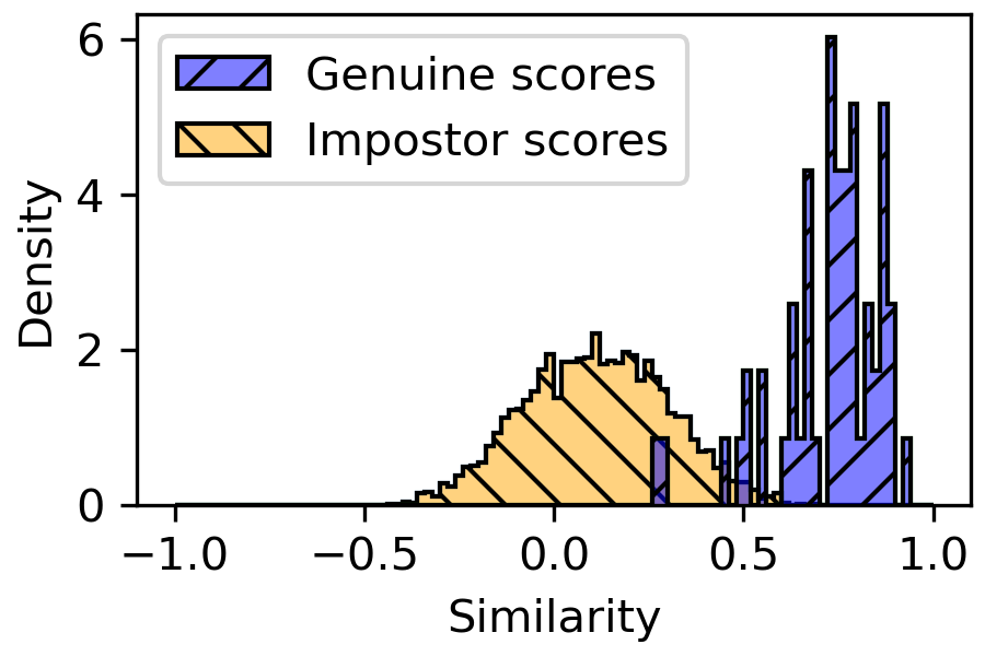
(A)

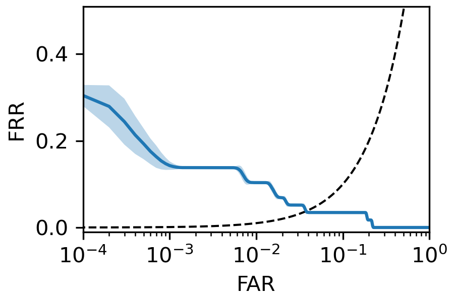
(B)

Figure 4: Qualitative results for the primary evaluation setting: 5 s of R1 TEX. (A) Genuine and impostor similarity score distributions. (B) ROC curve for bootstrapped similarity score distributions (see § V-E for an explanation of how the bootstrapped distributions are made). The dashed black line shows where FRR and FAR are equal. The blue line is the mean ROC curve across 1000 bootstrapped distributions, and the shaded region represents $\pm$1 standard deviation around the mean.

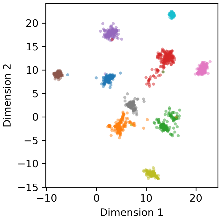
(A)

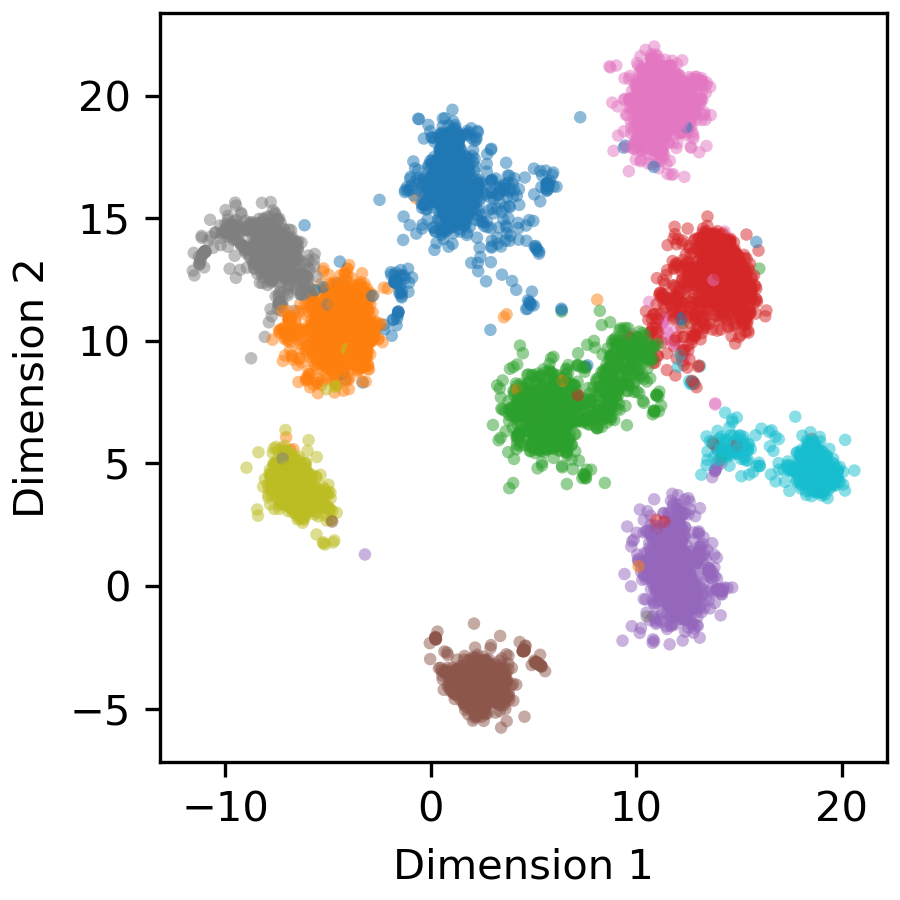
(B)

Figure 5: DensMAP [63] visualizations of the embedding space for 10 subjects present across all rounds. All embeddings of valid ($\leq$50% NaNs) windows across all rounds R1–9 and both sessions are plotted together. A different mapping is fit for each plot. (A) Embeddings from only the TEX task. (B) Embeddings from all tasks (including BLG). We use umap-learn [57] parameters metric=cosine, n_neighbors=30, min_dist=0.1, and densmap=True.

V-A Effect of task on authentication accuracy

For this analysis, we replace TEX with one of the other tasks during evaluation and repeat for each task. Note that we evaluate our single ensemble model across all tasks; we do not train a separate model for each task. Results are presented in Table I in the “Task” effect group. To assess our model’s performance on an out-of-sample task, we also include results for BLG.

V-B Effect of test-retest interval on authentication accuracy

For this analysis, we continue using the first session of R1 for the enrollment set, but for the authentication set we use the second session of one of the later rounds (R2–9) to assess how robust our model is to template aging after as many as 37 months. Results are presented in Table I in the “Test-retest interval” effect group.

V-C Effect of recording duration on authentication accuracy

For this analysis, instead of limiting ourselves to the first 5-second window of a recording, we aggregate embeddings across the first $n$ windows to form a new, centroid embedding. Since the model is trained to create a well-clustered embedding space, averaging multiple embeddings for a given class should lead to a better estimate of that class’s central tendency in the embedding space. Results are presented in Table I in the “Duration” effect group.

V-D Effect of sampling rate on authentication accuracy

For this analysis, instead of using 1000 Hz data, we downsample each recording to different target sampling rates using an anti-aliasing filter (SciPy’s [64] decimate function) to assess how robust our network architecture is to lower sampling rates. The targeted sampling rates are the same as those in [23]: 500, 250, 125, 50, and 31.25 Hz. Input size is reduced by the same integer factor as the sampling rate and then truncated to remove any fractional components. For example, at 31.25 Hz (a downsample factor of 32), the input size becomes $\lfloor\frac{5000}{32}\rfloor=156$ time steps.

Since our network architecture contains a global pooling layer prior to the fully-connected layer(s), the network can be applied to time series of any length without any modifications. But, because features learned at one sampling rate would not likely translate well to different sampling rates, we opted to train a new ensemble of 4-fold cross-validated models for each degraded sampling rate to have the best chance at extracting meaningful information at each sampling rate.

We do not adjust the Savitzky-Golay differentiation filter parameters for the lower sampling rates. It is also worth noting that the (maximum) receptive field of our network, 257 time steps, is larger than the input sizes at 50 and 31.25 Hz.

TABLE II: Biometric authentication results at degraded sampling rates. A different ensemble of models is trained for each sampling rate.

Sampling rate (Hz)	EER (%)	P	N
$500$	$5.66$	$53$	$3079$
$250$	$6.20$	$53$	$3079$
$125$	$8.77$	$57$	$3306$
$50$	$15.52$	$58$	$3364$
$31.25$	$23.37$	$58$	$3364$

V-E Estimating FRR @ FAR $10^{-4}$

The ultimate goal of EMB is to enable the use of eye movements for biometric authentication in real-world settings. It is important to consider how EMB compares to existing security methods, because if it cannot outperform such methods then wide adoption would be unlikely. Like [23], we use the 4-digit (10-key) pin as a representative for existing security methods, because it is one of the most common security methods in everyday life as both a primary and secondary security measure. The 4-digit pin effectively has a FAR of 1-in-10000, assuming each of the $10^{4}$ combinations of 4-digit 10-key pins is equally likely to be chosen by enrolled users.

For this analysis, to mimic the level of security afforded by a 4-digit pin, we provide estimates of FRR when FAR is fixed at $10^{-4}$ (abbreviated FRR @ FAR $10^{-4}$). Directly measuring FRR @ FAR $10^{-4}$ requires at least $\text{N}=10000$ impostor similarity scores, but we are limited to a maximum of 3422. Therefore, to enable the estimation of FRR @ FAR $10^{-4}$, we use bootstrapping (i.e., repeated random sampling with replacement) to resample our empirical genuine and impostor similarity score distributions to form new distributions with $\text{P}=20000$ and $\text{N}=20000$ scores. We repeat bootstrapping 1000 times and report the mean and standard deviation of the performance across those 1000 bootstrapped distributions. The FIDO Biometrics Requirements [65] suggest that a biometric system should have no higher than 3–5% FRR @ FAR $10^{-4}$, though we note that our bootstrapping technique differs from theirs and our test set population of 59 does not meet their minimum population requirements of 123–245.

TABLE III: Biometric authentication results using bootstrapped similarity score distributions. Results are reported as $\text{mean}_{\pm\text{SD}}$ across 1000 bootstrapped distributions. Each bootstrapped distribution contains $\text{P}=20000$ positives and $\text{N}=20000$ negatives.

Sampling rate (Hz)	Duration (s)	EER (%)	FRR @ FAR (%)
			$10^{-1}$	$10^{-2}$	$10^{-3}$	$10^{-4}$
$1000$	$5\times\hphantom{1}1$	$3.67_{\pm 0.12}$	$3.45_{\pm 0.13}$	$10.34_{\pm 0.22}$	$14.27_{\pm 1.04}$	$30.19_{\pm 2.87}$
	$5\times\hphantom{1}2$	$2.22_{\pm 0.11}$	$0.00_{\pm 0.00}$	$5.16_{\pm 0.19}$	$13.60_{\pm 1.78}$	$17.13_{\pm 0.50}$
	$5\times\hphantom{1}4$	$0.38_{\pm 0.05}$	$0.00_{\pm 0.00}$	$0.00_{\pm 0.00}$	$8.33_{\pm 0.73}$	$8.48_{\pm 0.20}$
	$5\times\hphantom{1}6$	$0.56_{\pm 0.05}$	$0.00_{\pm 0.00}$	$0.00_{\pm 0.00}$	$5.08_{\pm 0.16}$	$5.08_{\pm 0.16}$
	$5\times 12$	$0.59_{\pm 0.05}$	$0.00_{\pm 0.00}$	$0.00_{\pm 0.00}$	$5.09_{\pm 0.16}$	$5.09_{\pm 0.16}$
$500$	$5\times 12$	$0.32_{\pm 0.04}$	$0.00_{\pm 0.00}$	$0.00_{\pm 0.00}$	$3.82_{\pm 0.31}$	$7.46_{\pm 0.43}$
$250$		$0.81_{\pm 0.06}$	$0.00_{\pm 0.00}$	$0.00_{\pm 0.00}$	$3.78_{\pm 0.13}$	$5.58_{\pm 0.44}$
$125$		$3.49_{\pm 0.12}$	$0.00_{\pm 0.00}$	$7.02_{\pm 0.18}$	$10.47_{\pm 0.36}$	$10.52_{\pm 0.21}$
$50$		$3.38_{\pm 0.13}$	$0.00_{\pm 0.00}$	$10.40_{\pm 0.63}$	$16.06_{\pm 1.47}$	$20.21_{\pm 0.52}$
$31.25$		$5.09_{\pm 0.16}$	$5.09_{\pm 0.16}$	$14.47_{\pm 1.12}$	$29.36_{\pm 2.12}$	$51.28_{\pm 4.26}$

We note that EKY [23] employs a different method to estimate FRR @ FAR $10^{-4}$ involving the Pearson family of distributions. We propose the use of bootstrapping because it is simpler, makes fewer assumptions about the empirical distribution, and is more commonly used as a resampling tool. Bootstrapping largely preserves the shape of the empirical distribution, whereas the Pearson-based approach by [23] produces a new distribution that may not preserve characteristics of the region of interest where the genuine and impostor distributions overlap. A “failure case” of the Pearson-based approach is shown in Fig. 6. We believe the main source of this failure is that the empirical distribution of genuine scores is not unimodal (there appears to be a smaller second mode around 0.8 similarity), so we break the assumptions of the Pearson distribution.

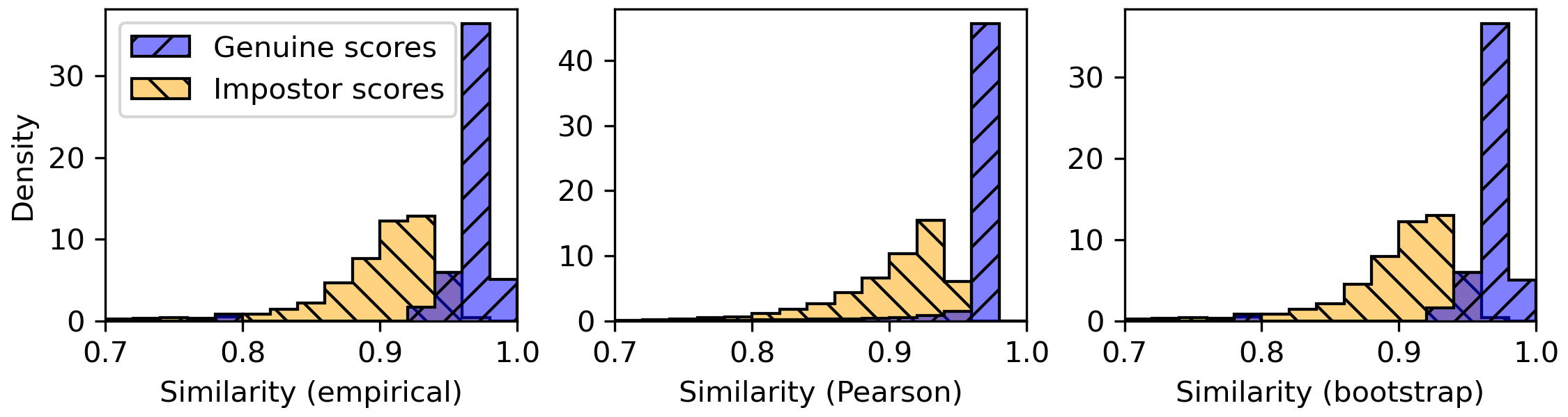
Figure 6: Comparison of genuine vs impostor similarity score distributions for (left) the empirical distributions, (center) resampled distributions using the Pearson-based method from [23], and (right) resampled distributions using bootstrapping. We note that bootstrapping more closely preserves the shape of the empirical distributions, particularly the overlapping region between the genuine and impostor distributions. In contrast, the Pearson-based method produces significantly less overlap between the genuine and impostor distributions, leading to a significant reduction in FRR @ FAR $10^{-4}$ compared to the bootstrapped distributions. Plotted scores are from evaluating our model on 31.25 Hz R1 TEX with $5\times 12$ inputs. In this example, the Pearson-based method results in 6.26% FRR @ FAR $10^{-4}$ which is significantly different from the bootstrapped result of 51.28%.

V-F Determining accept/reject threshold on validation set

As mentioned in [23], it is problematic to compute EER on the test set, because doing so leaks information from the test set into the decision of which accept/reject threshold to use. A more principled approach is to use the validation set to determine the accept/reject threshold and then apply that threshold to the test set.

For this analysis, we do exactly that. For each individual model from the ensemble, we build a ROC curve using similarity scores computed on that model’s validation set and determine the threshold that yields the EER. Then, separately for each model, we apply the chosen threshold on the similarity scores from the test set.

Note that for this analysis, unlike the previous analyses, we are no longer treating the 4 models as a single ensemble model, because each model’s validation set is present in the train set for the other 3 models. So, to provide a better understanding of performance without ensembling the individual models, we also measure EER for each individual model.

Results for this analysis are presented in Table IV. We label the folds F0, F1, F2, and F3 and match each model to the fold that was used as its validation set.

TABLE IV: Biometric authentication results on the test set for each individual model from the ensemble when the accept/reject threshold is determined on either the test set or a given model’s validation set.

Fold	Fit on test set		Fit on validation set
	threshold	EER (%)	threshold	FRR (%)	FAR (%)
F0	$0.4231$	$5.71$	$0.5405$	$12.07$	$1.28$
F1	$0.3970$	$8.62$	$0.5850$	$15.52$	$0.65$
F2	$0.4505$	$5.17$	$0.5575$	$10.34$	$1.25$
F3	$0.4277$	$6.90$	$0.5024$	$8.62$	$2.82$

V-G Comparison to previous state of the art

The statistical approach by Friedman et al. [45] reports 2.01% EER ($\text{P}=149$, $\text{N}=22052$) on the TEX task from GazeBase when enrolling with the full duration (approx. 60 s) of the first session of R1 and authenticating with the full duration (approx. 60 s) of the second session of R1. This result can be directly compared to our result of 0.58% EER ($\text{P}=59$, $\text{N}=3422$) for the $5\times 12$ duration in Table I in the “Duration” group.

EKY [23] reports 14.88% EER ($\text{P}=59$, $\text{N}=3422$) on the TEX task from GazeBase when enrolling with the first 5 s of the first session of R1 and authenticating with the first 5 s of the second session of R1. This result can be directly compared to our primary result in the first row of Table I where we achieve 3.66% EER ($\text{P}=58$, $\text{N}=3364$) under the same condition (except we exclude windows with more than 50% NaNs).

DEL [4] reports 10.0% EER ($\text{P}=25$, $\text{N}=600$) on the TEX task from GazeBase when enrolling with 24 s of data sampled from R1–2 and authenticating with 5 s of data sampled from R3–4. This result can be roughly compared to our results in Table I in the “Test-retest interval” group, particularly for R2–4, where we achieve between 7.43% and 8.71% EER ($\text{P}=58$, $\text{N}=3364$). Though, we note that we enroll with only the first 5 s of the first session of R1.

It is also worth briefly comparing against EKY and DEL at degraded sampling rates. DEL reports a mean EER of 9% with 5 s of 125 Hz data in [66]. This is similar to our result of 8.77% EER with 5 s of 125 Hz data, but it is difficult to directly compare across studies since we use a different dataset. EKY reports a mean EER of 18.75% with 10 s of 125 Hz data which is significantly worse than our results. We note that estimates of FRR @ FAR are not reported in [66].

For our final analysis, we evaluate our model on the JuDo1000 [67] dataset which is recorded with an eye-tracking device similar to the one used in GazeBase and which uses an eye-tracking task similar to the RAN task from GazeBase. JuDo1000 contains 150 subjects recorded across 4 sessions, each separated by at least 1 week. Each session contains 12 repetitions each of 9 different trial configurations. More details about the dataset can be found in [67].

From each recording, the 12 trials with the largest display area (grid = 0.25) and longest duration (dur = 1000) are selected, providing us with 12 windows of 5 s each. JuDo1000 is a binocular dataset but our model was trained on monocular data, so we combine the left and right eye gaze positions by averaging them. Gaze positions in each window are converted from pixels to degrees and then from position to velocity using the same Savitzky-Golay differentiation filter we used for GazeBase. Using the same trained model that produced the results shown in Table I and without any fine-tuning, we simply compute embeddings of these windows from JuDo1000. We enroll the embeddings from the first recording session and authenticate with the embeddings from the second recording session (a test-retest interval of approximately 1 week), excluding windows with more than 50% NaNs.

Table V shows our results alongside the published results of DEL. Since there are more than 10000 negative pairs, FRR @ FAR $10^{-4}$ is directly measured without any resampling. We note that this is not a one-to-one comparison with DEL for several reasons, including: DEL trained on JuDo1000 but we trained on GazeBase; DEL used a total of 12 input channels but we used 2; DEL enrolled using 24 s of data across 3 recording sessions but we enrolled with 5 s from only 1 session; and DEL averages results across all 9 trial configurations in JuDo1000 but we only use 1 trial configuration. That said, these results show the robustness of our model to completely out-of-sample data.

TABLE V: Biometric authentication results on the JuDo1000 [67] dataset.

Model	Duration (s)	EER (%)	FRR @ FAR (%)		P	N
			$10^{-2}$	$10^{-4}$
DEL [4]	$1\times\hphantom{1}5$	$3.97$	$25.67$	-	$25$	$600$
	$1\times 10$	$3.01$	$22.01$	-	$25$	$600$
Ours*	$5\times\hphantom{1}1$	$12.00$	$44.00$	$92.00$	$150$	$22\,350$
	$5\times\hphantom{1}2$	$7.33$	$28.67$	$68.67$	$150$	$22\,350$
	$5\times 12$	$2.67$	$5.33$	$24.00$	$150$	$22\,350$
* Our model was trained on GazeBase and evaluated on JuDo1000.

VI Discussion

The primary result that we present is 3.66% EER on a reading task with 5-second-long enrollment and authentication periods and with an approximately 30-minute test-retest interval. eky [23] reports a mean EER of 14.88% under similar conditions. del [4] reports a mean EER of 3.97% on a jumping dot task with an enrollment period lasting 24 seconds over a 3-week period and a 5-second-long authentication period with an approximately 1-week test-retest interval.

Authentication accuracy is generally better for TEX than the other tasks, as is expected given the literature’s predominant use of reading data for EMB. The EER for VD2 is slightly lower than for TEX, but this difference may not be statistically significant and the trend may not continue for longer durations. Unsurprisingly, authentication accuracy is the worst for FXS; but it is impressive that we manage to achieve below 10% EER given just 5 s of pure fixational data. We note that the FXS task was not well represented in the training set, because the task has a maximum duration of approx. 15 s (compared to 60–100 s for the other tasks) and all other tasks are likely to elicit several saccadic movements in any given 5-second period. What is quite surprising, however, is that our model achieves 5.49% EER on BLG despite that task not being present during training. BLG presumably elicits very different eye movement responses than the other tasks because it is an interactive game with many objects moving on the screen at once, but our model is still able to create meaningful embeddings of the eye movement signals. We also draw attention to the fact that the embedding space (Fig. 5B) appears to be fairly well-clustered across tasks, suggesting that it may be viable to enroll with one task and authenticate with another.

Our model exhibits high robustness to template aging, even with just 5 s of eye movement data. When authenticating on R6, which is approx. 1 year after R1 and is not represented in the train or validation sets, we still achieve 6.09% EER. In fact, EER remains consistently between 6–9% for all test-retest intervals from approx. 1 to 37 months.

It is still an open question as to how much eye movement data is necessary to adequately perform user authentication and whether there is a point beyond which additional data provides no new information. For our model, EER improves as the duration of enrollment and authentication increases from 5 s to 20 s, after which it starts to saturate around 0.4–0.6%. Estimates of FRR @ FAR $10^{-4}$ improve with increasing duration up to 30 s before saturating around 5%. Our results suggest that there may not be much additional information to be gained beyond 30 s of eye movements during a reading task. Though, it must be noted that this claim is based on the TEX task from GazeBase wherein each subject read through each passage at different speeds. Perhaps the reason we do not see much improvement beyond 30 s is that most subjects may have finished reading after 30 s and did not have consistent behavior afterward.

Authentication accuracy remains relatively stable as the sampling rate is degraded from 1000 Hz down to 250 Hz, starts to noticeably worsen at 125 Hz, and then drops significantly starting at 50 Hz. It is unclear how much of this performance degradation is due to the use of an untuned differentiation filter. These results may reflect findings in the literature that saccade characteristics (e.g., peak velocity and duration) can be measured accurately at a sampling rate of 250 Hz [68] and begin to become less accurate at lower sampling rates [69, 70]. At 125 Hz, which is close to the 120 Hz sampling rate of the Vive Pro Eye [14], our model is still able to achieve 8.77% EER with just 5 s of data and an estimated 10.52% FRR @ FAR $10^{-4}$ with 60 s of data. Depending on the degree of security necessary, these results suggest the present applicability of EMB at sampling rates present in current VR/AR devices. Another interesting observation is that we are able to achieve around 5.09% EER with 60 s of 31.25 Hz data, suggesting that there is still meaningful biometric information that can be extracted at such low sampling rates. While we acknowledge that simply degrading the sampling rate of high-quality data is not a sufficient proxy for other eye-tracking devices, we note that gaze estimation pipelines could always be improved to produce higher levels of signal quality at a particular sampling rate, whereas it may not always be possible for a device to increase the sampling rate of its eye-tracking sensor(s) due to power constraints (though some efforts are being made to enable eye tracking at high sampling rates with lower power requirements [18]).

Most EMB studies, including the present study, report measures of EER directly on the test set, leaking information from the test set into the accept/reject decisions. When taking a more principled approach and fitting the accept/reject threshold on the validation set instead, we find that the thresholds become more strict, resulting in a lower FAR and a higher FRR. As such, these thresholds would be better for settings requiring a higher degree of security but may be more frustrating for users.

VII Conclusion

We presented a novel, highly parameter-efficient, DenseNet-based architecture for end-to-end EMB that achieves state-of-the-art biometric authentication performance. When enrolling and authenticating with just 5 s of eye movements during a reading task—a duration somewhat comparable to the time it takes to enter a 4-digit pin or to calibrate an eye-tracking device—we achieved 3.66% EER. With 30 s of data, we achieved an estimated 5.08% FRR @ FAR $10^{-4}$ which approaches a level of authentication performance that would be acceptable for real-world use. At 125 Hz, which is close to the 120 Hz sampling rate of the Vive Pro Eye [14], we achieved 8.77% EER with just 5 s of data and an estimated 10.52% FRR @ FAR $10^{-4}$ with 60 s of data.

Our embedding space visualizations suggest that it may be feasible to enroll with one (or several) tasks and authenticate with a different task. We are not aware of any study that has attempted this. It would also be interesting to see how well privacy-preserving models (e.g., [12]) can defend against more powerful EMB models like the one presented herein.

Since eye tracking is seeing increasing use in VR/AR devices due in part to the power-saving potential of foveated rendering, EMB may be an ideal biometric modality for such devices. emb models would need to have low resource requirements when performing (continuous) user authentication on such consumer-grade devices. Our architecture (excluding the classification layer) has only 123K learnable parameters which is around 4x smaller than EKY (approx. 475K learnable parameters) and around 1700x smaller than DEL (approx. 209M learnable parameters according to [23]). Models with lower complexity such as ours may enable more power-efficient implementations that would make them a better fit for deployment on consumer-grade devices. Following works like [19], we encourage future studies to explore EMB directly on eye-tracking-enabled VR/AR devices.

References

- [1] A. Jain, A. Ross, and S. Prabhakar, “An introduction to biometric recognition,” IEEE Transactions on Circuits and Systems for Video Technology, vol. 14, no. 1, pp. 4–20, 2004.
- [2] P. Kasprowski and J. Ober, “Eye movements in biometrics,” Lecture Notes in Computer Science (including subseries Lecture Notes in Artificial Intelligence and Lecture Notes in Bioinformatics), vol. 3087, pp. 248–258, 2004.
- [3] O. V. Komogortsev, A. Karpov, and C. D. Holland, “Attack of mechanical replicas: Liveness detection with eye movements,” IEEE Transactions on Information Forensics and Security, vol. 10, no. 4, pp. 716–725, 2015.
- [4] S. Makowski, P. Prasse, D. R. Reich, D. Krakowczyk, L. A. Jäger, and T. Scheffer, “Deepeyedentificationlive: Oculomotoric biometric identification and presentation-attack detection using deep neural networks,” IEEE Transactions on Biometrics, Behavior, and Identity Science, vol. 3, no. 4, pp. 506–518, 2021.
- [5] S. Eberz, K. Rasmussen, V. Lenders, and I. Martinovic, “Preventing lunchtime attacks: Fighting insider threats with eye movement biometrics,” 2015.
- [6] S. Eberz, G. Lovisotto, K. B. Rasmussen, V. Lenders, and I. Martinovic, “28 Blinks Later: Tackling Practical Challenges of Eye Movement Biometrics,” in Proceedings of the 2019 ACM SIGSAC Conference on Computer and Communications Security, ser. CCS ’19. London, United Kingdom: Association for Computing Machinery, Nov. 2019, pp. 1187–1199. [Online]. Available: https://doi.org/10.1145/3319535.3354233
- [7] P. Kasprowski and K. Harezlak, “Fusion of eye movement and mouse dynamics for reliable behavioral biometrics,” Pattern Analysis and Applications, vol. 21, no. 1, pp. 91–103, Feb. 2018. [Online]. Available: https://doi.org/10.1007/s10044-016-0568-5
- [8] O. V. Komogortsev, A. Karpov, C. D. Holland, and H. P. Proença, “Multimodal ocular biometrics approach: A feasibility study,” in 2012 IEEE Fifth International Conference on Biometrics: Theory, Applications and Systems (BTAS), 2012, pp. 209–216.
- [9] D. J. Liebling and S. Preibusch, “Privacy considerations for a pervasive eye tracking world.” Association for Computing Machinery, Inc, 2014, pp. 1169–1177.
- [10] A. Liu, L. Xia, A. Duchowski, R. Bailey, K. Holmqvist, and E. Jain, “Differential privacy for eye-tracking data,” Proceedings of the 11th ACM Symposium on Eye Tracking Research & Applications, p. 10, 2019. [Online]. Available: https://doi.org/10.1145/3314111.3319823
- [11] J. Steil, I. Hagestedt, M. X. Huang, and A. Bulling, “Privacy-aware eye tracking using differential privacy.” ACM, 6 2019, pp. 1–9. [Online]. Available: https://dl.acm.org/doi/10.1145/3314111.3319915
- [12] B. David-John, D. Hosfelt, K. Butler, and E. Jain, “A privacy-preserving approach to streaming eye-tracking data,” IEEE Transactions on Visualization and Computer Graphics, 2021. [Online]. Available: https://www.nytimes.com/interactive/2019/12/19/opinion/
- [13] J. Li, A. R. Chowdhury, K. Fawaz, and Y. Kim, “Kaleido: Real-time privacy control for eye-tracking systems,” 2021.
- [14] “Vive Pro Eye,” https://www.vive.com/us/product/vive-pro-eye/overview/, accessed: 2021-04-07.
- [15] “Magic Leap 1,” https://www.magicleap.com/en-us/magic-leap-1, accessed: 2021-04-07.
- [16] “HoloLens 2,” https://www.microsoft.com/en-us/hololens, accessed: 2022-03-27.
- [17] B. Guenter, M. Finch, S. Drucker, D. Tan, and J. Snyder, “Foveated 3d graphics,” ACM Trans. Graph., vol. 31, no. 6, nov 2012. [Online]. Available: https://doi.org/10.1145/2366145.2366183
- [18] T. Stoffregen, H. Daraei, C. Robinson, and A. Fix, “Event-based kilohertz eye tracking using coded differential lighting,” in 2022 IEEE/CVF Winter Conference on Applications of Computer Vision (WACV), 2022, pp. 3937–3945.
- [19] D. J. Lohr, S. Aziz, and O. Komogortsev, “Eye movement biometrics using a new dataset collected in virtual reality,” in ACM Symposium on Eye Tracking Research and Applications, ser. ETRA ’20 Adjunct. New York, NY, USA: Association for Computing Machinery, 2020. [Online]. Available: https://doi.org/10.1145/3379157.3391420
- [20] S. Jia, D. H. Koh, A. Seccia, P. Antonenko, R. Lamb, A. Keil, M. Schneps, and M. Pomplun, “Biometric recognition through eye movements using a recurrent neural network,” in Proceedings - 9th IEEE International Conference on Big Knowledge, ICBK 2018. Institute of Electrical and Electronics Engineers Inc., dec 2018, pp. 57–64.
- [21] A. Abdelwahab and N. Landwehr, “Deep Distributional Sequence Embeddings Based on a Wasserstein Loss,” arXiv:1912.01933 [cs, stat], Dec. 2019, arXiv: 1912.01933. [Online]. Available: http://arxiv.org/abs/1912.01933
- [22] L. A. Jäger, S. Makowski, P. Prasse, S. Liehr, M. Seidler, and T. Scheffer, “Deep eyedentification: Biometric identification using micro-movements of the eye,” in Machine Learning and Knowledge Discovery in Databases, U. Brefeld, E. Fromont, A. Hotho, A. Knobbe, M. Maathuis, and C. Robardet, Eds. Cham: Springer International Publishing, 2020, pp. 299–314.
- [23] D. Lohr, H. Griffith, and O. V. Komogortsev, “Eye know you: Metric learning for end-to-end biometric authentication using eye movements from a longitudinal dataset,” 2021.
- [24] K. He, X. Zhang, S. Ren, and J. Sun, “Deep residual learning for image recognition,” 2015.
- [25] G. Huang, Z. Liu, L. van der Maaten, and K. Q. Weinberger, “Densely connected convolutional networks,” 2018.
- [26] H. Griffith, D. Lohr, E. Abdulin, and O. Komogortsev, “Gazebase, a large-scale, multi-stimulus, longitudinal eye movement dataset,” Scientific Data, vol. 8, no. 1, p. 184, Jul 2021. [Online]. Available: https://doi.org/10.1038/s41597-021-00959-y
- [27] L. Friedman, H. S. Stern, V. Prokopenko, S. Djanian, H. K. Griffith, and O. V. Komogortsev, “Biometric performance as a function of gallery size,” 2020.
- [28] J. Unar, W. C. Seng, and A. Abbasi, “A review of biometric technology along with trends and prospects,” Pattern Recognition, vol. 47, no. 8, pp. 2673–2688, 2014. [Online]. Available: https://www.sciencedirect.com/science/article/pii/S003132031400034X
- [29] A. Krizhevsky, I. Sutskever, and G. E. Hinton, “Imagenet classification with deep convolutional neural networks,” in Advances in Neural Information Processing Systems, F. Pereira, C. J. C. Burges, L. Bottou, and K. Q. Weinberger, Eds., vol. 25. Curran Associates, Inc., 2012. [Online]. Available: https://proceedings.neurips.cc/paper/2012/file/c399862d3b9d6b76c8436e924a68c45b-Paper.pdf
- [30] K. Simonyan and A. Zisserman, “Very deep convolutional networks for large-scale image recognition,” 2015.
- [31] C. Elmadjian, C. Gonzales, and C. H. Morimoto, “Eye movement classification with temporal convolutional networks,” in Pattern Recognition. ICPR International Workshops and Challenges, A. Del Bimbo, R. Cucchiara, S. Sclaroff, G. M. Farinella, T. Mei, M. Bertini, H. J. Escalante, and R. Vezzani, Eds. Cham: Springer International Publishing, 2021, pp. 390–404.
- [32] A. van den Oord, S. Dieleman, H. Zen, K. Simonyan, O. Vinyals, A. Graves, N. Kalchbrenner, A. Senior, and K. Kavukcuoglu, “Wavenet: A generative model for raw audio,” in Arxiv, 2016. [Online]. Available: https://arxiv.org/abs/1609.03499
- [33] S. Hochreiter and J. Schmidhuber, “Long Short-Term Memory,” Neural Computation, vol. 9, no. 8, pp. 1735–1780, 11 1997. [Online]. Available: https://doi.org/10.1162/neco.1997.9.8.1735
- [34] K. Cho, B. van Merrienboer, C. Gulcehre, D. Bahdanau, F. Bougares, H. Schwenk, and Y. Bengio, “Learning phrase representations using rnn encoder-decoder for statistical machine translation,” 2014.
- [35] C. Lea, R. Vidal, A. Reiter, and G. D. Hager, “Temporal convolutional networks: A unified approach to action segmentation,” 2016.
- [36] H. Li, Z. Xu, G. Taylor, C. Studer, and T. Goldstein, “Visualizing the loss landscape of neural nets,” 2018.
- [37] S. Xie, R. Girshick, P. Dollár, Z. Tu, and K. He, “Aggregated residual transformations for deep neural networks,” 2017.
- [38] C. Zhang, P. Benz, D. M. Argaw, S. Lee, J. Kim, F. Rameau, J.-C. Bazin, and I. S. Kweon, “Resnet or densenet? introducing dense shortcuts to resnet,” 2020.
- [39] M. Tan and Q. V. Le, “Efficientnet: Rethinking model scaling for convolutional neural networks,” 2020.
- [40] ——, “Efficientnetv2: Smaller models and faster training,” 2021.
- [41] A. Vaswani, N. Shazeer, N. Parmar, J. Uszkoreit, L. Jones, A. N. Gomez, L. u. Kaiser, and I. Polosukhin, “Attention is all you need,” in Advances in Neural Information Processing Systems, I. Guyon, U. V. Luxburg, S. Bengio, H. Wallach, R. Fergus, S. Vishwanathan, and R. Garnett, Eds., vol. 30. Curran Associates, Inc., 2017. [Online]. Available: https://proceedings.neurips.cc/paper/2017/file/3f5ee243547dee91fbd053c1c4a845aa-Paper.pdf
- [42] A. Dosovitskiy, L. Beyer, A. Kolesnikov, D. Weissenborn, X. Zhai, T. Unterthiner, M. Dehghani, M. Minderer, G. Heigold, S. Gelly, J. Uszkoreit, and N. Houlsby, “An image is worth 16x16 words: Transformers for image recognition at scale,” in International Conference on Learning Representations, 2021. [Online]. Available: https://openreview.net/forum?id=YicbFdNTTy
- [43] C. Holland and O. V. Komogortsev, “Biometric identification via eye movement scanpaths in reading,” in 2011 International Joint Conference on Biometrics (IJCB), 2011, pp. 1–8.
- [44] A. George and A. Routray, “A score level fusion method for eye movement biometrics,” Pattern Recogn. Lett., vol. 82, no. P2, p. 207–215, oct 2016. [Online]. Available: https://doi.org/10.1016/j.patrec.2015.11.020
- [45] L. Friedman, M. S. Nixon, and O. V. Komogortsev, “Method to assess the temporal persistence of potential biometric features: Application to oculomotor, gait, face and brain structure databases,” PLOS ONE, vol. 12, no. 6, pp. 1–42, 06 2017. [Online]. Available: https://doi.org/10.1371/journal.pone.0178501
- [46] D. Lohr, H. Griffith, S. Aziz, and O. Komogortsev, “A metric learning approach to eye movement biometrics,” in 2020 IEEE International Joint Conference on Biometrics (IJCB), 2020, pp. 1–7.
- [47] M. Porta, P. Dondi, N. Zangrandi, and L. Lombardi, “Gaze-based biometrics from free observation of moving elements,” IEEE Transactions on Biometrics, Behavior, and Identity Science, vol. 4, no. 1, pp. 85–96, 2022.
- [48] S. Ioffe and C. Szegedy, “Batch normalization: Accelerating deep network training by reducing internal covariate shift,” in Proceedings of the 32nd International Conference on Machine Learning, ser. Proceedings of Machine Learning Research, F. Bach and D. Blei, Eds., vol. 37. Lille, France: PMLR, 07–09 Jul 2015, pp. 448–456. [Online]. Available: https://proceedings.mlr.press/v37/ioffe15.html
- [49] V. Nair and G. E. Hinton, “Rectified linear units improve restricted boltzmann machines,” in Proceedings of the 27th International Conference on International Conference on Machine Learning, ser. ICML’10. Madison, WI, USA: Omnipress, 2010, p. 807–814.
- [50] K. He, X. Zhang, S. Ren, and J. Sun, “Delving deep into rectifiers: Surpassing human-level performance on imagenet classification,” 2015. [Online]. Available: https://arxiv.org/abs/1502.01852
- [51] K. Wan, S. Yang, B. Feng, Y. Ding, and L. Xie, “Reconciling feature-reuse and overfitting in densenet with specialized dropout,” in 2019 IEEE 31st International Conference on Tools with Artificial Intelligence (ICTAI), 2019, pp. 760–767.
- [52] K. He, X. Zhang, S. Ren, and J. Sun, “Identity mappings in deep residual networks,” 2016.
- [53] A. Paszke, S. Gross, F. Massa, A. Lerer, J. Bradbury, G. Chanan, T. Killeen, Z. Lin, N. Gimelshein, L. Antiga, A. Desmaison, A. Kopf, E. Yang, Z. DeVito, M. Raison, A. Tejani, S. Chilamkurthy, B. Steiner, L. Fang, J. Bai, and S. Chintala, “Pytorch: An imperative style, high-performance deep learning library,” in Advances in Neural Information Processing Systems 32, H. Wallach, H. Larochelle, A. Beygelzimer, F. d'Alché-Buc, E. Fox, and R. Garnett, Eds. Curran Associates, Inc., 2019, pp. 8024–8035. [Online]. Available: http://papers.neurips.cc/paper/9015-pytorch-an-imperative-style-high-performance-deep-learning-library.pdf
- [54] K. Musgrave, S. Belongie, and S.-N. Lim, “Pytorch metric learning,” 2020.
- [55] W. Falcon and The PyTorch Lightning team, “PyTorch Lightning,” 3 2019. [Online]. Available: https://github.com/PyTorchLightning/pytorch-lightning
- [56] L. Biewald, “Experiment tracking with weights and biases,” 2020, software available from wandb.com. [Online]. Available: https://www.wandb.com/
- [57] L. McInnes, J. Healy, N. Saul, and L. Grossberger, “Umap: Uniform manifold approximation and projection,” The Journal of Open Source Software, vol. 3, no. 29, p. 861, 2018.
- [58] A. Savitzky and M. J. E. Golay, “Smoothing and differentiation of data by simplified least squares procedures.” Analytical Chemistry, vol. 36, no. 8, pp. 1627–1639, 1964. [Online]. Available: https://doi.org/10.1021/ac60214a047
- [59] X. Wang, X. Han, W. Huang, D. Dong, and M. R. Scott, “Multi-similarity loss with general pair weighting for deep metric learning,” in 2019 IEEE/CVF Conference on Computer Vision and Pattern Recognition (CVPR), 2019, pp. 5017–5025.
- [60] D. P. Kingma and J. Ba, “Adam: A method for stochastic optimization,” arXiv preprint arXiv:1412.6980, 2014.
- [61] L. N. Smith and N. Topin, “Super-convergence: Very fast training of neural networks using large learning rates,” 2018.
- [62] K. Musgrave, S. Belongie, and S.-N. Lim, “A metric learning reality check,” in Computer Vision – ECCV 2020, A. Vedaldi, H. Bischof, T. Brox, and J.-M. Frahm, Eds. Cham: Springer International Publishing, 2020, pp. 681–699.
- [63] A. Narayan, B. Berger, and H. Cho, “Density-preserving data visualization unveils dynamic patterns of single-cell transcriptomic variability,” bioRxiv, 2020. [Online]. Available: https://www.biorxiv.org/content/early/2020/05/14/2020.05.12.077776
- [64] P. Virtanen, R. Gommers, T. E. Oliphant, M. Haberland, T. Reddy, D. Cournapeau, E. Burovski, P. Peterson, W. Weckesser, J. Bright, S. J. van der Walt, M. Brett, J. Wilson, K. J. Millman, N. Mayorov, A. R. J. Nelson, E. Jones, R. Kern, E. Larson, C. J. Carey, İ. Polat, Y. Feng, E. W. Moore, J. VanderPlas, D. Laxalde, J. Perktold, R. Cimrman, I. Henriksen, E. A. Quintero, C. R. Harris, A. M. Archibald, A. H. Ribeiro, F. Pedregosa, P. van Mulbregt, and SciPy 1.0 Contributors, “SciPy 1.0: Fundamental Algorithms for Scientific Computing in Python,” Nature Methods, vol. 17, pp. 261–272, 2020.
- [65] S. Schuckers, G. Cannon, and N. Tekampe, “FIDO biometrics requirements,” https://fidoalliance.org/specs/biometric/requirements/, accessed: 2021-04-04.
- [66] P. Prasse, L. A. Jäger, S. Makowski, M. Feuerpfeil, and T. Scheffer, “On the relationship between eye tracking resolution and performance of oculomotoric biometric identification,” vol. 176. Elsevier, 1 2020, pp. 2088–2097.
- [67] S. Makowski, L. A. Jäger, P. Prasse, and T. Scheffer, “Biometric identification and presentation-attack detection using micro- and macro-movements of the eyes,” in 2020 IEEE International Joint Conference on Biometrics (IJCB), 2020, pp. 1–10.
- [68] J. van der Geest and M. Frens, “Recording eye movements with video-oculography and scleral search coils: a direct comparison of two methods,” Journal of Neuroscience Methods, vol. 114, no. 2, pp. 185–195, 2002. [Online]. Available: https://www.sciencedirect.com/science/article/pii/S0165027001005271
- [69] R. Andersson, M. Nyström, and K. Holmqvist, “Sampling frequency and eye-tracking measures: how speed affects durations, latencies, and more,” Journal of Eye Movement Research, vol. 3, no. 3, Sep. 2010. [Online]. Available: https://bop.unibe.ch/JEMR/article/view/2300
- [70] A. Leube and K. Rifai, “Sampling rate influences saccade detection in mobile eye tracking of a reading task,” Journal of eye movement research, vol. 10, no. 3, p. 10.16910/jemr.10.3.3, Jun 2017, 33828659[pmid]. [Online]. Available: https://pubmed.ncbi.nlm.nih.gov/33828659