Implementing simple spectral denoising for environmental audio recordings

Abstract

This technical report details changes applied to a noise filter to facilitate its application and improve its results. The filter is applied to denoise natural sounds recorded in the wild and to generate an acoustic index used in soundscape analysis.

1 Introduction

Signal distortions and noise are often present in real-life audio acquisition. In environmental audio recordings, background noise is even more evident due to the capture in the wild. When it comes to using the recordings as input to recognition systems, noise and distortions can impair accurate ecological interpretations of acoustic features.

In ecological analysis via audio data, for example, as presented by Dias et al. [1], Dröge et al. [2], Gan et al. [3], Hilasaca et al. [4], Scarpelli et al. [5], acoustic features have an important role in the task of summarizing, representing, visualizing, and analyzing soundscapes. Therefore, removing noise from an audio signal is an important pre-processing step to extract and analyze proper acoustic features related to soundscape dynamics. Moreover, techniques as source separation are also used to help that analysis [6, 7].

In this report, we describe the denoising procedure proposed by Towsey [8]. We also aim at improving its performance and simplicity through the application of a simple algorithm to generate the noise profile and the threshold used in the algorithm.

2 Basic concepts

In this section, we describe the original filter implementation, the threshold selection approach, and a statistical tool used to identify and remove outliers.

2.1 Spectral filtering

There are several filters available that are designed to be more general or serve specific denoising purposes. Among those techniques, the subtraction methods are considered to be straightforward. In particular, the subtraction using mean, median, or mode are often employed [8]. In this report, we present a filter developed by Towsey [8], which uses modal noise subtraction and assumes that the signal is generated by the addition of acoustic events energy with a Gaussian background noise. We focused on a filter in the frequency domain, but a similar process can be used on the time domain.

Towsey [8] created a variation of the adaptive level equalisation method [9], which assumes an additive Gaussian model, described in Algorithm 1. First, the algorithm uses histograms to identify the mode value of each spectrogram band frequency and generate a noise profile of the spectrum. In the next step, a smoothed profile is subtracted from the spectrogram rows and negative values are truncated to zero. Towsey [8] implemented an additional step that preserves complex events such as bird vocalizations. They slide a window throughout the filtered spectrogram, calculating the mean and the minimum values of the region under the window. If the mean is lower than a user-defined threshold, the minimum value is assigned to the spectrogram position where the window is centered.

Algorithm 1 Noise removal from spectrograms proposed by Towsey [8]

1:  Input signal $\mathbf{s}$ and threshold $\theta$

2:  $Sxx\leftarrow\text{stft}(\mathbf{s},window=Hamming,size=512,hop=256)$

3:  $S\leftarrow\text{abs}(Sxx)$ {Step A}

4:  $profile\leftarrow\emptyset$

5:  for  $i\leftarrow 1$ to $\#rows(S)$  do

6:     $h\leftarrow\text{histogram}(S_{i},bins=100)$

7:     $h\leftarrow\text{moving\_average}(h,window=5)$

8:     $M\leftarrow bin_{j}$ with max $h_{j}$

9:     if  $j>95$  then

10:        $M\leftarrow bin_{95}$

11:     Insert $M$ in the $profile$ {Step B}

12:  $profile\leftarrow\text{moving\_average}(profile,window=5)$

13:  for  $i\leftarrow 1$ to #rows($S$)  do

14:     for  $j\leftarrow 1$ to #cols($S$)  do

15:        $S_{ij}\leftarrow S_{ij}-profile_{i}$

16:        if  $S_{ij}<0$  then

17:           $S_{ij}\leftarrow 0$ {Step C (additional)}

18:  Centered in each $S_{ij}$ position, slide a $w_{9\times 3}$ window throughout $S$

19:  and calculate $avg_{ij}$ and $min_{ij}$ of the area under $w$.

20:  if  $avg_{ij}<\theta$  then

21:     $S_{ij}\leftarrow min_{ij}$

22:  

23:  Output abs(istft($S\circ Sxx$)) {$\circ$ is the element-wise product}

2.2 Threshold selection

A recurring task in image processing and analysis is the definition of a threshold to separate foreground from the image background [10] that can be applied to image binarization and segmentation even as a post-processing step [11]. Otsu [10] developed a non-parametric and unsupervised approach to encounter a suitable threshold for these tasks. Assuming the data is bimodal, i.e., it is distributed so that there are two main distinct parts or classes (in images usually foreground and background), the technique attempts to maximize the modal/class separability, evaluating the between-class variance ($\sigma_{B}^{2}$), iterating over the range values to encounter the better threshold $k$, by:

$$\max_{1\leq k<L}\sigma_{B}^{2}(k),$$

where $L=255$ in a gray-scale image scenario. Considering the values of the image histogram as $p_{i}$, it is possible to define the probability of $C_{0}$ (class before the threshold $k$) as $\omega(k)=\sum_{i=1}^{k}p_{i}$, and the mean of that class as $\mu(k)=\sum_{i=1}^{k}ip_{i}$. The total mean can be calculated as $\mu_{T}=\sum_{i=1}^{L}ip_{i}$. In that way, the between-class variance could be expressed as:

$$\sigma_{B}^{2}(k)=\frac{[\mu_{T}\omega(k)-\mu(k)]^{2}}{\omega(k)[1-\omega(k)]}.$$

2.3 Statistical quartiles

A quartile is a statistical term used when an ordered range is divided into four parts and the Boxplot chart, generally employed in data analyses, is a suitable visualization that uses such information [12]. Thus, we have the first quartile $Q_{1}$ representing the number that limits the first 25% values, the second quartile $Q_{2}$ limits the 50% of the range (the median), and the third quartile $Q_{3}$ limits the 75% of the range. Furthermore, it is possible to calculate a dispersion measure named interquartile range $IQR=Q_{3}-Q_{1}$ that can be used to identify the limit range values. Almost 99.3% of the range stays between the lower limit ($Q_{1}-1.5\times IQR$) and the higher limit ($Q_{3}+1.5\times IQR$). The remaining values (outside the range) are named as outliers.

3 Denoising method updated

We implemented two adaptations in the Algorithm 1. First, the noise profile (lines 4-11) is defined by the automatic threshold selection as defined in section 2.2. We assume there are two modes on a given frequency band, the foreground sounds and the background noise, and that a proper noise profile $M$ is the value that better describe the separation between these modes, what could generate a refined profile to distinct situations.

With the tool described in section 2.3, we remove outlier values from the band frequencies to avoid their impact into the process. We iteractively identify and remove the values beyond lower and higher limits, until no outlier is encountered. Then, we generate the histogram of the remaining values and also apply a moving average (Algorithm 1, lines 6-7), and finally search for the threshold as described in section 2.2. In this case, $bin$ represents real numbers, instead of integers between $[0,255]$ as in image context.

The second modification is on the definition of the $\theta$ parameter, since it depends on previous knowledge of the audio set and it can be complex to tune. Hence, we applied the previous outliers exclusion and threshold search to the average values $avg$ calculated by Algorithm 1 (lines 18-19), and used it as $\theta$ parameter. Finally, we also rescale the signal s to $[-1,1]$ range before the filtering process and after the reconstruction of the signal we rescale the result to the original signal range. That rescale improved filtering of low volume sounds.

4 Background noise index

With the same process used to remove noise in section 3, we updated the Background noise index (BGN). The noise profile generated is the spectral version of the BGN (named as BGN_sp) and the summary index BGN is the application of the process (removing outliers and searching threshold) to the Hilbert amplitude envelope of the audio signal. Before the calculation, as described by Towsey [8], we also convert values to decibel and truncate them to -90 dB when they are lesser than this value (truncation can not be necessary).

5 Experimental results

This section presents some tests with our implementations. We considered two clips with 30 seconds from two recordings with distinct attributes and collected under different approaches, one audio file from a terrestrial area and another from an underwater area. Both audio files are from the dataset used by Dias et al. [1].

1(a) presents a terrestrial recording and its respective filtered versions (original and new filter). The recording has mainly biophony sounds, such as birds and insects, and geophony sounds such as heavy rain starting after 5 seconds. There are great differences between filtered and non-filtered signals and the distinction between filter versions is easiest to verify up to 12 seconds, where our approach removed more rain noise. In 1(b), the profile yielded by the new filter has a larger range, which can explain the better cleaning presented with the spectrograms. We also analyzed the sound to noise ratio (SNR) [13] and the BGN index (see section 4), both calculated for each second of the recordings. SNR is calculated as the relation between the mean and standard deviation of the power spectral density (PSD) [14] of the audio signal. Curves in Figure 2 follow the same ascending patterns and the new filter generated a signal with SNR mean lesser than the original filter (0.12 and 0.13, respectively). Related to BGN, the new filter attained a greater mean than the original filter (37.27 and 26.44, respectively).

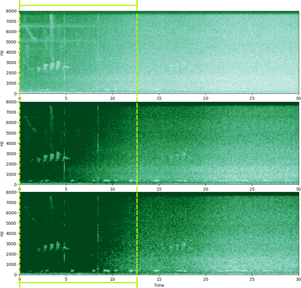
(a) Spectrogram results

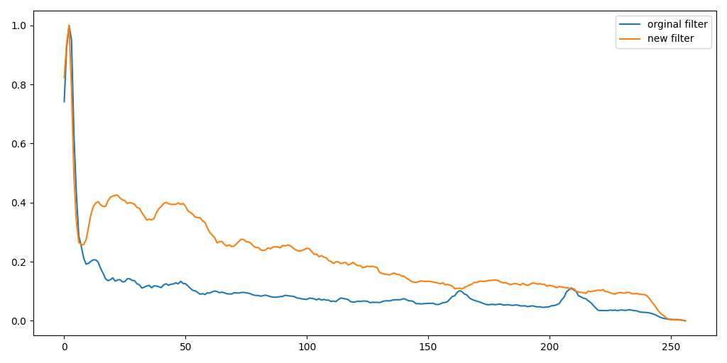
(b) Noise profiles of filters

Figure 1: (a) Spectrograms of the terrestrial recording (top), its filtered version (middle) with the original filter, and its filtered version (bottom) with the new filter. In the highlighted area (up to 12 seconds), the differences between the results of the filters are more perceptible. (b) Noise profile (BGN_sp) generated by the filter versions. Values were normalized to present curves in a suitable view

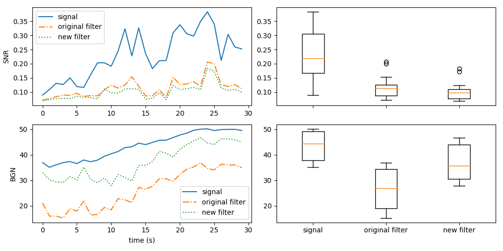
Figure 2: Acoustic features of the terrestrial sound signal and the filtered signal with filter versions. Values calculated for each file second

On the other hand, filters results in the underwater recording are very similar, which can be verified with the inspection of Figure 3 and Figure 4. That recording contains mainly humpback whale and fish choruses. Curves in Figure 4 are monotonic, SNR mean of the signal with the new filter is lesser than with the original filter (0.1494 and 0.1513, respectively), and BGN mean of the signal with the new filter is also lesser than the signal BGN mean with the original filter (42.57 and 43.70, respectively).

6 Final Remarks

Following those simple tests, the new implementation did not damage the application of the spectral filter and enhanced the estimation of BGN values. The new filter removed more noise (rain) of terrestrial recording than its older version because the generated noise profile could better represent frequency noise related to stationary sound such as rain. When applied to underwater recording, the new filter attained similar noise attenuation to its old version. Constant sounds as fish chorus were preserved, probably owing to frequency variations and overlaps with whale vocalizations. It is noteworthy that an approach developed to filter terrestrial sounds can be applied to other cases such as underwater.

Finally, our modifications presented straightforward and suitable ways to automatically define and tune the algorithm parameters, maintaining or improving the denoising results. Furthermore, we recommend tests with other foreground sounds and background noise to assess the algorithm’s robustness.

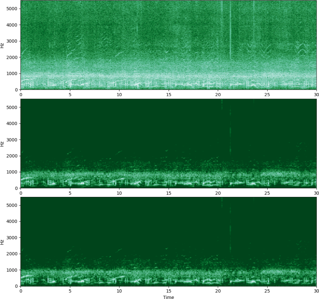
(a) Spectrogram results

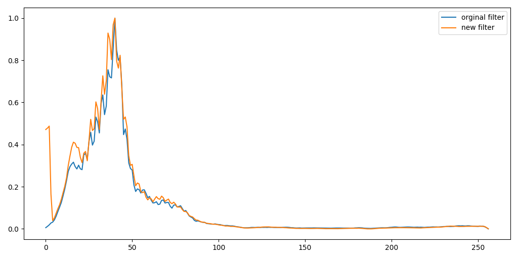
(b) Noise profiles of filters

Figure 3: (a) Spectrograms of the underwater recording (top), its filtered version (middle) with the original filter, and its filtered version (bottom) with the new filter. (b) Noise profile (BGN_sp) generated by the filter versions. Values were normalized to present curves in a suitable view

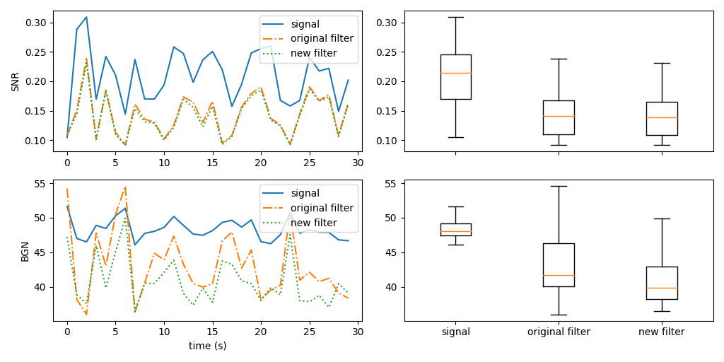
Figure 4: Acoustic features of the underwater sound signal and the filtered signal with filter versions. Values calculated for each file second

References

- Dias et al. [2021] F. F. Dias, H. Pedrini, R. Minghim, Soundscape segregation based on visual analysis and discriminating features, Ecological Informatics 61 (2021) 101184.
- Dröge et al. [2021] S. Dröge, D. A. Martin, R. Andriafanomezantsoa, Z. Burivalova, T. R. Fulgence, K. Osen, E. Rakotomalala, D. Schwab, A. Wurz, T. Richter, et al., Listening to a changing landscape: Acoustic indices reflect bird species richness and plot-scale vegetation structure across different land-use types in north-eastern madagascar, Ecological Indicators 120 (2021) 106929.
- Gan et al. [2020] H. Gan, J. Zhang, M. Towsey, A. Truskinger, D. Stark, B. J. van Rensburg, Y. Li, P. Roe, Data selection in frog chorusing recognition with acoustic indices, Ecological Informatics 60 (2020) 101160.
- Hilasaca et al. [2021] L. M. H. Hilasaca, L. P. Gaspar, M. C. Ribeiro, R. Minghim, Visualization and categorization of ecological acoustic events based on discriminant features, Ecological Indicators 126 (2021) 107316.
- Scarpelli et al. [2021] M. D. Scarpelli, M. C. Ribeiro, C. P. Teixeira, What does atlantic forest soundscapes can tell us about landscape?, Ecological Indicators 121 (2021) 107050.
- Lin et al. [2017] T.-H. Lin, S.-H. Fang, Y. Tsao, Improving biodiversity assessment via unsupervised separation of biological sounds from long-duration recordings, Scientific reports 7 (2017) 4547.
- Lin and Tsao [2020] T.-H. Lin, Y. Tsao, Source separation in ecoacoustics: A roadmap towards versatile soundscape information retrieval, Remote Sensing in Ecology and Conservation 6 (2020) 236–247.
- Towsey [2017] M. W. Towsey, The calculation of acoustic indices derived from long-duration recordings of the natural environment, 2017. URL: https://eprints.qut.edu.au/110634/.
- Lamel et al. [1981] L. Lamel, L. Rabiner, A. Rosenberg, J. Wilpon, An improved endpoint detector for isolated word recognition, IEEE Transactions on Acoustics, Speech, and Signal Processing 29 (1981) 777–785.
- Otsu [1979] N. Otsu, A threshold selection method from gray-level histograms, IEEE transactions on systems, man, and cybernetics 9 (1979) 62–66.
- Ponti [2012] M. P. Ponti, Segmentation of low-cost remote sensing images combining vegetation indices and mean shift, IEEE Geoscience and Remote Sensing Letters 10 (2012) 67–70.
- Frigge et al. [1989] M. Frigge, D. C. Hoaglin, B. Iglewicz, Some implementations of the boxplot, The American Statistician 43 (1989) 50–54.
- Bedoya et al. [2017] C. Bedoya, C. Isaza, J. M. Daza, J. D. López, Automatic identification of rainfall in acoustic recordings, Ecological indicators 75 (2017) 95–100.
- Welch [1967] P. Welch, The use of fast fourier transform for the estimation of power spectra: a method based on time averaging over short, modified periodograms, IEEE Transactions on Audio and Electroacoustics 15 (1967) 70–73.