Reduced Order Modeling of Turbulence-Chemistry Interactions using Dynamically Bi-Orthonormal Decomposition

Abstract

The performance of the dynamically bi-orthogonal (DBO) decomposition for the reduced order modeling of turbulence-chemistry interactions is assessed. DBO is an on-the-fly low-rank approximation technique, in which the instantaneous composition matrix of the reactive flow field is decomposed into a set of orthonormal spatial modes, a set of orthonormal vectors in the composition space, and a factorization of the low-rank correlation matrix. Two factors which distinguish between DBO and the reduced order models (ROMs) based on the principal component analysis (PCA) are: (i) DBO does not require any offline data generation; and (ii) in DBO the low-rank composition subspace is time-dependent as opposed to static subspaces in PCA. Because of these features, DBO can adapt on-the-fly to intrinsic and externally excited transient changes in state of the transport variables. For demonstration, simulations are conducted of a non-premixed CO/H₂ flame in a temporally evolving jet. The GRI-Mech 3.0 model with 53 species is used for chemical kinetics modeling. The results are appraised via a posteriori comparisons against data generated via full-rank direct numerical simulation (DNS) of the same flame, and the PCA reduction of the DNS data. The DBO also yields excellent predictions of various statistics of the thermo-chemical variables.

  Keywords: Reduced order modeling, time-dependent basis, dynamically bi-orthonormal decomposition.  

1 Introduction

One of the most significant challenges with turbulent combustion modeling and simulation is associated with the high dimensionality of the transport variables as required for its physical description [1, 2, 3]. Hydrocarbon combustion, for example, involves from 50 to 7000 species depending on the fuel [4, 5]. Even with the aid of exascale computing, high-fidelity simulations of turbulent reactive flows with detailed kinetic remain computationally prohibitive [6, 7]. To deal with this issue, developments of reduced ordered models (ROMs) have been at the heart of turbulent reacting flow research for many decades now [8, 2]. Most of the current methods are for development of low order manifolds by which all other transport variables can be calculated.

Consider the species mass fractions field $\bm{\Phi}(x,t)\equiv\big{[}\phi_{1}(x,t)\big{|}\phi_{2}(x,t)\big{|}\dots\big{|}\phi_{n_{s}}(x,t)\big{]}$ for $n_{s}$ total number of species, with $(x,t)$ denoting the space-time coordinates. The earliest, the simplest, and still one of the most popular models is the flame sheet approximation in which the statistics of all of the thermo-chemical variables are related to those of a single conserved variable: the mixture fraction [9, 10, 11] (${\cal Z}(x,t)$). The same is the case for flows under chemical equilibrium: $\phi_{\alpha}(x,t)=\phi_{\alpha}({\cal Z}(x,t))$. The simplest extension is the Laminar Flamelet Model (LFM), in which another variable is augmented to the mixture fraction. $\phi_{\alpha}(x,t)=\phi_{\alpha}({\cal Z}(x,t),{\cal X}(x,t))$, where the choice of the auxiliary ${\cal X}(x,t)$ variable depends on the flame structure. The model originally due to Peters [12], has been one of the most popular means of turbulent combustion simulation for several decades now. For some examples, see Refs. [13, 14, 15, 16, 17, 18, 19, 20, 21, 22, 23]. This popularity is partially due to the model’s simplicity. However, the joint statistics of the mixture fraction and the auxiliary variable cannot be specified in a systematic manner [24].

Developments of higher order manifolds via reduced order kinetics have been the subjects of broad investigations by a variety of methods [4, 2]. In these methods, essentially the composition variables are partitioned into a set of represented (reduced) compositions, and the remaining unrepresented ones. The manifold is constructed as a multivariate function of a small number of the reduced compositions. The construction is either based on the original thermo-chemistry equations with imposition of certain assumptions about their physical-chemical characteristics, or empirically by analysis of the data generated via detailed chemistry for a given flow. Both of these approaches have experienced success. However, they are all optimized for specific flow conditions or configurations. It would be desired to have the manifold reduction technique developed on-the-fly for general applications.

Exploiting various correlations via dimensionality reduction is one way to reduce the computational burden of solving turbulent reactive transport equations. See Refs. [25, 26] for the application of principal component analysis (PCA) in turbulent combustion. The dimension reduction techniques exploit the correlated structure in the data and they seek the intrinsic dimensionality by transforming the high-dimensional data into a meaningful representation of reduced dimensionality [27, 28]. While dimensionality reduction techniques are widely used for analysis and data compression [29, 30, 31, 32, 33, 34, 35, 36], or to build ROMs [37], they share one important feature: They extract the low-rank structure from data and they are designed for a target problem. To reduce the number of species on-the-fly, one approach is to extract these structures from the model, i.e. reactive species transport equations and bypass the need to generate data. Recently, some of these techniques, which we refer to as model-driven dimension reduction techniques, have shown promising results for the solution of stochastic partial differential equations (PDEs). Dynamically orthogonal (DO) [38, 39, 40], bi-orthogonal (BO) [41] and dynamically bi-orthonormal decompositions (DBO) [42, 43] are model-driven stochastic ROM techniques. For deterministic linear dynamical systems, optimally time-dependent (OTD) reduction was introduced [44, 45]. In all of these model-driven techniques, closed-form (partial) differential equations for the evolution of the low rank structures (modes) are derived. Leveraging the mathematical rigour of these techniques, for some cases, numerical and dynamical system analyses are used to shed light into their performance and dynamics [46, 47, 48]. Closely related techniques can also be found in quantum physics and quantum chemistry [49, 50].

The objective of this work is to develop and implement our model-driven strategy [43] to systematically construct reduced order modeling of turbulence-chemistry interactions in a canonical flow. The developments is not under any restrictive flow assumption, but is in conjunction with direct numerical simulation (DNS) in which the lower dimension subspace of the representative fields are constructed on-the-fly.

2 Methodology

2.1 Formulation

For a variable density reacting flow involving $n_{s}$ species, the primary transport variables are the fluid density $\rho(x,t)$, the velocity vector $\bm{v}(x,t)$, the specific enthalpy $h(x,t)$, the pressure $p(x,t)$, and the species mass fractions $\phi_{\alpha}(x,t)\ (\alpha=1,2,\dots,n_{s})$. The conservation equations governing the transport variables are the continuity, momentum, enthalpy (energy) and species mass fraction equations, along with an equation of state in the format detailed in Ref. [51]. The transport equations for composition space (species mass fractions and enthalpy) can be stated in the matrix form as:

$$\frac{\partial\Phi}{\partial t}=-(\bm{v}\cdot\nabla)\Phi+\frac{1}{\rho}\nabla\cdot(\nabla\Phi\Gamma)+S(\rho,\Phi),$$ (1)

where $\Phi(x,t)\in\mathbb{R}^{\infty\times n_{c}}$ is the composition matrix with $n_{c}$ columns $(n_{c}=n_{s}+1)$, and $\infty$ denotes the continuous direction $(x)$:

$$\Phi(x,t)=[\phi_{1}(x,t) \mid\phi_{2}(x,t)\mid\dots$$

$$\dots \mid\phi_{n_{s}}(x,t)\mid\phi_{n_{c}}(x,t)],$$ (2)

in which $\phi_{n_{c}}\equiv h$. In Eq. (1), $\Gamma\in\mathbb{R}^{n_{c}\times n_{c}}=\mbox{diag}\{\gamma_{1},\gamma_{2},\dots,\gamma_{n_{c}}\}$ is the diagonal matrix of diffusivities at each spatial point, and $S$ denotes the chemical source term. The inner product in the spatial domain between two fields $f(x)$ and $g(x)$ is defined as:

$$\big{<}f(x),g(x)\big{>}=\int_{D}f(x)g(x)dx,$$

where $D$ denoted the physical domain, and the $L_{2}$ norm induced by this inner product as:

$$\big{\|}f(x)\big{\|}_{2}=\big{<}f(x),f(x)\big{>}^{\frac{1}{2}}.$$

The Frobenius norm of a matrix $A(x)=[a_{1}(x),a_{2}(x),\dots,a_{m}(x)]\in\mathbb{R}^{\infty\times m}$ is defined as:

$$\big{\|}A(x)\big{\|}_{\mathcal{F}}^{2}=\sum_{i=1}^{m}\int_{D}a_{i}^{2}(x)dx.$$

A column-wise inner product between two matrices $A(x,t)\in\mathbb{R}^{\infty\times m}$ and $B(x,t)\in\mathbb{R}^{\infty\times n}$ is defined as

$$Q(t)=\big{<}A(x,t),B(x,t)\big{>},$$

where $Q(t)\in\mathbb{R}^{m\times n}$ is a matrix with components $Q_{ij}(t)=\big{<}a_{i}(x,t),b_{j}(x,t)\big{>}$, where $b_{j}(x,t)$ denotes the $j$th column of $B(x,t)$. Therefore, $\big{<}AR_{A},B\big{>}=R_{A}^{T}\big{<}A,B\big{>}$ and $\big{<}A,BR_{B}\big{>}=\big{<}A,B\big{>}R_{B}$ for any $R_{A}\in\mathbb{R}^{m\times m}$ and $R_{B}\in\mathbb{R}^{n\times n}$.

The goal is to solve for a low-rank decomposition of $\Phi(x,t)$ instead of solving Eq. (1). To this end, the DBO decomposition for the full species concentration matrix is considered:

$$\Phi(x,t)=\sum_{j=1}^{r}\sum_{i=1}^{r}u_{i}(x,t)\Sigma_{ij}(t)y^{T}_{j}(t)+E(x,t),$$ (3)

where

$$U(x,t) =[u_{1}(x,t)\mid u_{2}(x,t)\mid...\mid u_{r}(x,t)],$$ (4a)

$$Y(t) =[y_{1}(t)\mid y_{2}(t)\mid...\mid y_{r}(t)].$$ (4b)

Here, $r<n_{c}$ is the reduction size, $U(x,t)\in\mathbb{R}^{\infty\times r}$ is a matrix whose columns are a set of time-dependent orthonormal spatial modes, $\Sigma(t)\in\mathbb{R}^{r\times r}$ is a factorization of the reduced correlation matrix, $Y(t)\in\mathbb{R}^{n_{c}\times r}$ is the matrix of time-dependent orthonormal composition modes, and $E(x,t)\in\mathbb{R}^{\infty\times n_{c}}$ is the reduction error. The key observation regarding Eq. (3) is that all three components are time dependent. This enables the decomposition to adapt on-the-fly to the changes in $\Phi(x,t)$. In fact, the DBO decomposition closely approximates the instantaneous singular value decomposition (SVD) of $\Phi(x,t)$. Orthonormality of spatial modes and composition modes implies that:

$$\big{<}u_{i}(x,t),u_{j}(x,t)\big{>}=\delta_{ij},$$ (5a)

$$y^{T}_{i}(t)y_{j}(t)=\delta_{ij},$$ (5b)

where $\delta_{ij}$ is the Kronecker delta. The variational principle whose optimality conditions lead to closed form evolution equations for the components of the DBO decomposition is given by:

$$\mathcal{F}(\dot{U},\dot{\Sigma},\dot{Y})=\left\|\frac{\partial}{\partial t}[U\Sigma Y^{T}]-\mathcal{M}(U\Sigma Y^{T})\right\|_{\mathcal{F}}^{2},$$ (6)

subject to the orthonormality conditions as given by Eqs. (5a)-(5b). In Eq. (6), $\dot{(~{})}\equiv\partial(~{})/\partial t$ and $\mathcal{M}$ is the right hand side of composition transport equation: $\mathcal{M}=-(\bm{v}\cdot\nabla)U\Sigma Y^{T}+\frac{1}{\rho}\nabla\cdot(\nabla U\Sigma Y^{T}\Gamma)+S(\rho,U\Sigma Y^{T})$. The variational principle given in Eq. (6) seeks to minimize the difference between the right hand side of the species transport equation and the time derivative of the DBO decomposition subject to the orthonormality constraints given by Eqs. (5a)-(5b). The control parameters are $\dot{U}$, $\dot{Y}$ and $\dot{\Sigma}$. As derived in Ref. [43], the closed-form evolution equations of $U(x,t)$, $\Sigma(t)$ and $Y(t)$ are:

$$\frac{\partial U}{\partial t} =(\mathcal{M}Y-U\big{<}U,\mathcal{M}Y\big{>})\Sigma^{-1},$$ (7a)

$$\frac{d\Sigma}{dt} =\big{<}U,\mathcal{M}Y\big{>},$$ (7b)

$$\frac{dY}{dt} =(I-YY^{T})\big{<}\mathcal{M},U\big{>}\Sigma^{-T}.$$ (7c)

2.2 Computational Cost

The main computational advantage of using DBO is to evolve only $r$ spatial modes (Eq. (7a)) instead of $n_{c}$ composition transport equations (Eq. (1)). The computational cost of evolving $\Sigma$ and $Y$ is negligible as they are governed by low-rank ordinary differential equations (ODEs). Moreover, in the DBO decomposition, the compositions are stored in the compressed form, i.e., matrices $U$, $\Sigma$ and $Y$ are kept in the memory as opposed to their multiplication $U\Sigma Y^{T}$, i.e., the decompressed form. The memory storage requirement is dominated by $U$ as $\Sigma$ and $Y$ are low-rank matrices and their storage cost is negligible. Therefore, in comparison to the full species transport equation, this results in the memory compression ratio of $n_{c}/r$. Reference [43] discusses the efficient way of calculating each terms on the right-hand-side of Eq. (7).

2.3 Comparison against DNS & PCA

The canonical representation of DBO is used for comparison against DNS and PCA. In this representation, the spatial and composition modes are ranked based on their “energy” in the second-norm sense. The ranking can be achieved by performing SVD of $\Sigma(t)$:

$$\Sigma(t)=R_{U}(t)\tilde{\Sigma}(t)R_{Y}(t),$$ (8)

where $\tilde{\Sigma}(t)$ is a diagonal matrix that contains the ranked singular values: $\tilde{\sigma}_{1}(t)>\tilde{\sigma}_{2}(t)>...>\tilde{\sigma}_{r}(t)$ and $R_{U}(t)$ and $R_{Y}(t)$ are orthonormal matrices that can be used to rotate $U$ and $Y$ as follows:

$$\tilde{U}(x,t) =U(x,t)R_{U}(t),$$ (9a)

$$\tilde{Y}(t) =Y(t)R_{Y}(t).$$ (9b)

The components $\{\tilde{U}(x,t),\tilde{\Sigma}(t),\tilde{Y}(t)\}$ represent the DBO decomposition in the canonical form. It is noted that the DBO in the canonical form, and the form that is computed are equivalent: $U\Sigma Y^{T}=\tilde{U}\tilde{\Sigma}\tilde{Y}^{T}$.

The results via DBO are compared with those generated by the reduction based on the instantaneous principal component analysis (I-PCA). The I-PCA components are calculated in a data-driven manner (based on DNS data) by computing SVD of the instantaneous matrix of full species: $\Phi(x,t)=\hat{U}(x,t)\hat{\Sigma}(t)\hat{Y}^{T}(t)$, where $\hat{(~{})}$ denotes the components of I-PCA, $\hat{U}(x,t)=\{\hat{u}_{1}(x,t),\hat{u}_{2}(x,t),\dots,\hat{u}_{n_{c}}(x,t)\}$ is the matrix of left singular functions, $\hat{\Sigma}(t)=\mbox{diag}(\hat{\sigma}_{1}(t),\hat{\sigma}_{2}(t),\dots,\hat{\sigma}_{n_{c}}(t))$ is the diagonal matrix of singular values and $\hat{Y}(t)=\{\hat{y}_{1}(t),\hat{y}_{2}(t),\dots,\hat{y}_{n_{c}}(t)\}$ is the matrix of right singular vectors.

The composition modes of PCA are static, and are derived by the SVD of the whole composition data from DNS through all time steps (not instantaneously like I-PCA) and spatial locations.

$$\mbox{PCA:}\quad\Phi(x,t) \simeq U_{PCA}(x,t)Y_{PCA}^{T},$$ (10a)

$$\mbox{DBO:}\quad\Phi(x,t) \simeq U(x,t)\Sigma(t)Y(t)^{T}.$$ (10b)

Equation (10) shows the contrast between time-dependent subspace extracted by DBO, and the static manifolds extracted from PCA. It should be emphasized that $Y_{PCA}$ is comparable with $Y(t)\Sigma(t)$ from DBO. Please refer to [43] for more details.

3 Flow Configuration and Model Specifications

For demonstration, the canonical configuration of a temporally developing planar CO/H₂ jet flame is considered. This flame has been the subject of previous detailed DNS [52], and several subsequent modeling and simulations [53, 54, 55, 56, 57, 51]. The flame is rich with strong flame-turbulence interactions resulting in local extinction followed by re-ignition. The configuration as considered here is the two-dimensional version of that in Ref. [52] and is depicted in Fig. 1. The jet consists of a central fuel stream of width $H=0.72$mm surrounded by counter-flowing oxidizer streams. The fuel stream is comprised of 50$\%$ of CO, 10$\%$ H₂ and 40$\%$ N₂ by volume, while oxidizer streams contain 75$\%$ N₂ and 25$\%$ O₂. The initial temperature of both streams is 500K and thermodynamic pressure is set to 1 atm. The velocity difference between the two streams is $U=145$m/s. The fuel stream velocity and the oxidizer stream velocity are $U/2$ and $-U/2$, respectively. The initial conditions for the velocity components and mixture fraction are taken directly from center-plane DNS in Ref. [52], and then the spatial fields of species and temperature are reconstructed from flamelet table generated with $\chi=0.75\chi_{\text{crit}}$, where $\chi$ and $\chi_{\text{crit}}$ are scalar dissipation rate and its critical value respectively. The boundary conditions are periodic in stream wise ($x$) and cross-stream wise ($y$) directions. The Reynolds number, based on $U$ and $H$ is $Re=2510$. The sound speeds in the fuel and the oxidizer streams are denoted by $C_{1}$ and $C_{2}$, respectively and the Mach number $Ma=U/\left(C_{1}+C_{2}\right)\approx 0.16$ is small enough to justify a low Mach number approximation. The combustion chemistry is modelled via the GRI-Mech 3.0 mechanism [58] containing 53 species with 325 reaction steps. The DNS of the base reactive flow is conducted via the PeleLM solver [59] as detailed in Ref. [51]. Simulations are conducted for the duration $0\leq t\leq 60t_{j}$, $t_{j}=H/U$, and the mixture fraction field, denoted by $Z(x,t)$ is constructed from the simulated data [60].

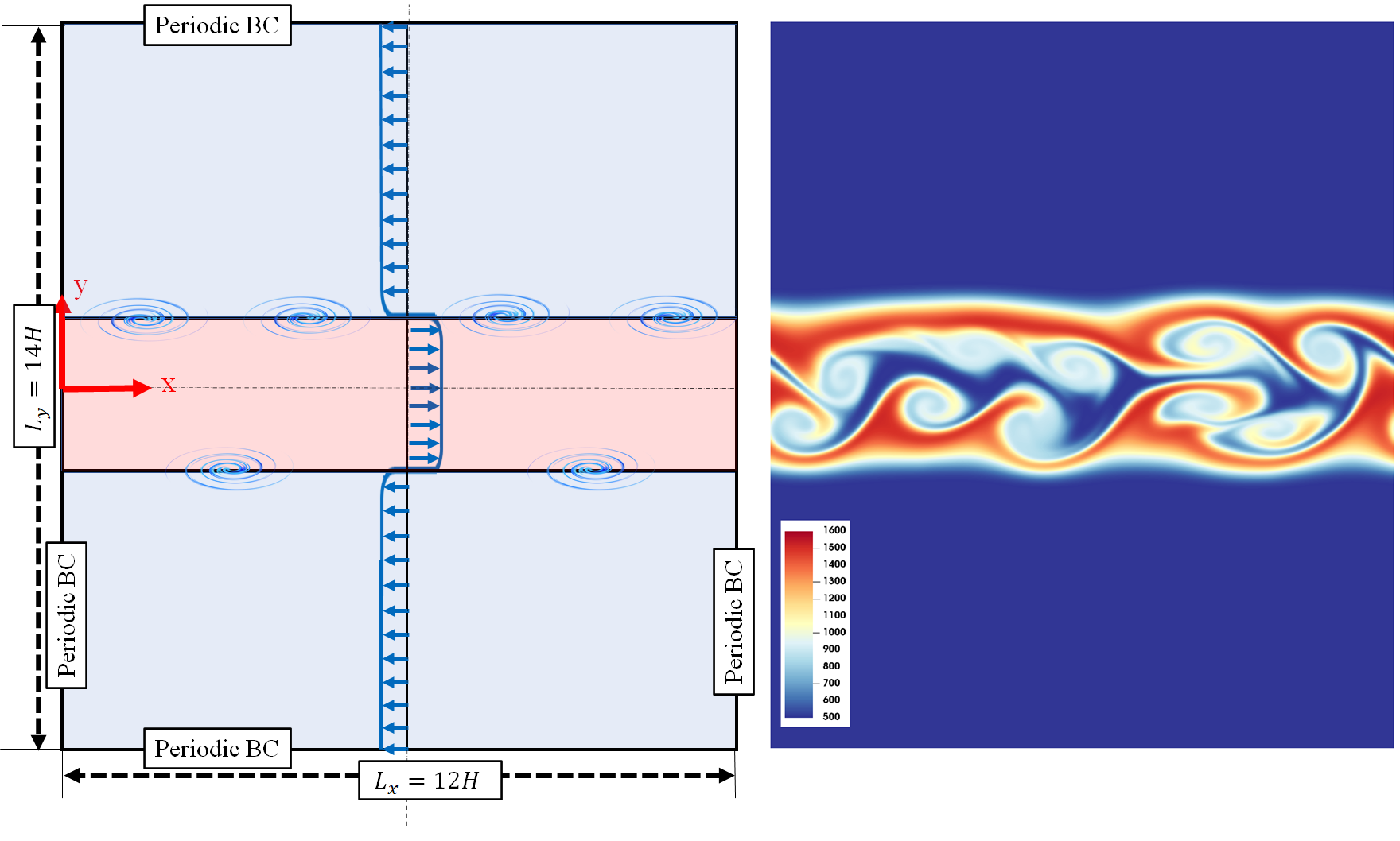
Fig. 1: Schematics of the temporally developing turbulent jet flame.

4 Results and Discussions

Two DBO-ROMs with ranks $r=6$ and $r=8$ are considered in conjunction with GRI-Mech 3.0 mechanism. In Fig. 2, the low-rank composition subspace is shown for I-PCA, PCA, and DBO. In particular, the absolute values of the first three dominant modes are shown. The species with very small $Y$ values are eliminated for clarity. The PCA and I-PCA are both extracted from the DNS data. It is observed that the PCA subspace is static, but the DBO subspace evolves with time. The subspace extracted by DBO matches well with the low-rank subspace extracted by I-PCA, which is the optimal instantaneous subspace in the $L_{2}$ sense. The main difference between the PCA and DBO is that in the former the composition subspace ($Y_{PCA}$) extracts low-rank structures in a time-averaged sense. In fact, $Y_{PCA}$ are the dominant eigenvectors of the space- and time-averaged correlation matrix constructed from the DNS data. The DBO composition subspace can change temporally and can closely approximate the eigenvectors of the instantaneous correlation matrix, as it is evidenced by a good agreement between $Y_{I-PCA}$ and $Y_{DBO}$. The DBO reduction does not require any data, and all of its components ($U$, $\Sigma$ and $Y$) are extracted directly from the composition transport equations (Eqs. (7a-7c)).

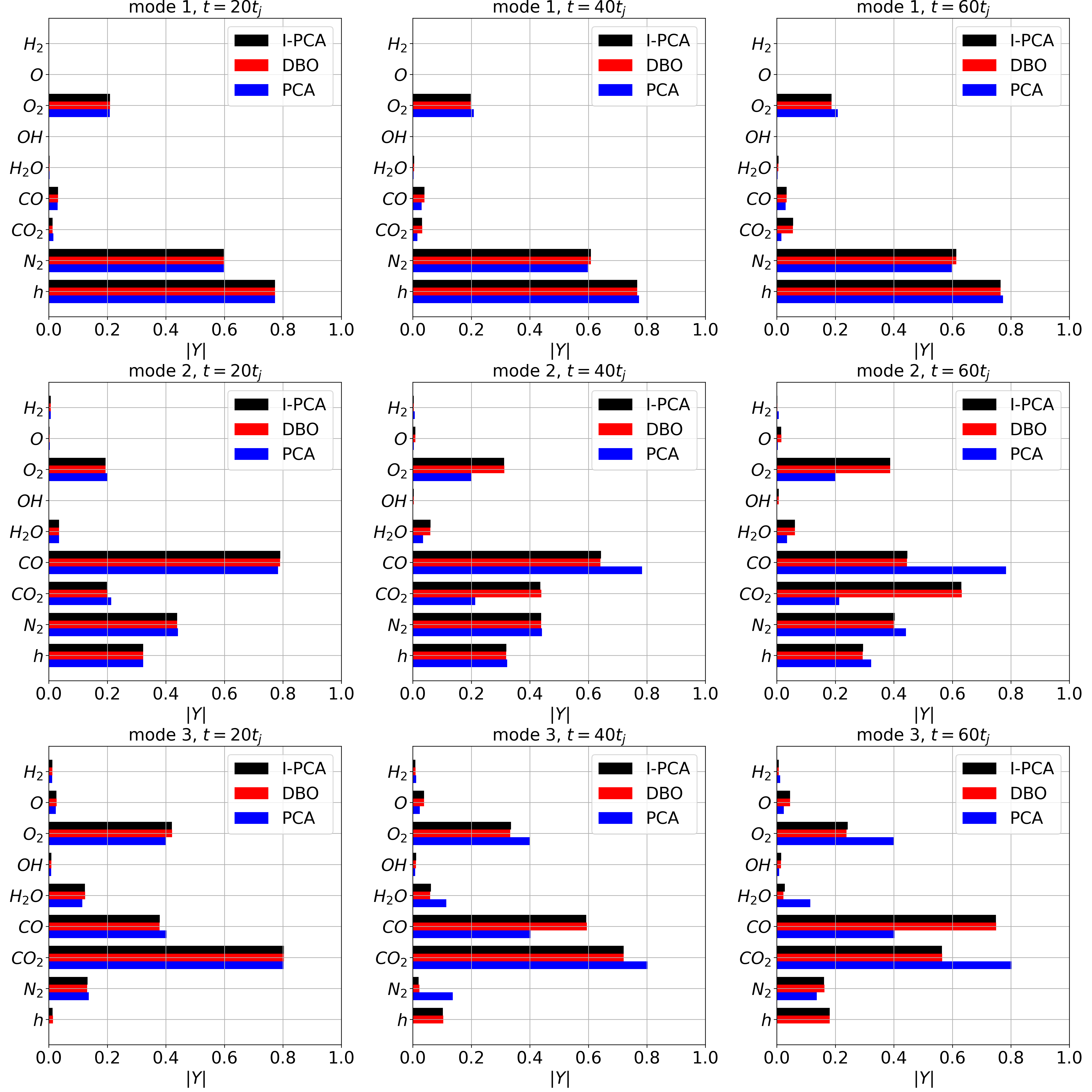
Fig. 2: Temporal evolution of species modes $Y$. For clarity, only most dominant scalars are shown.

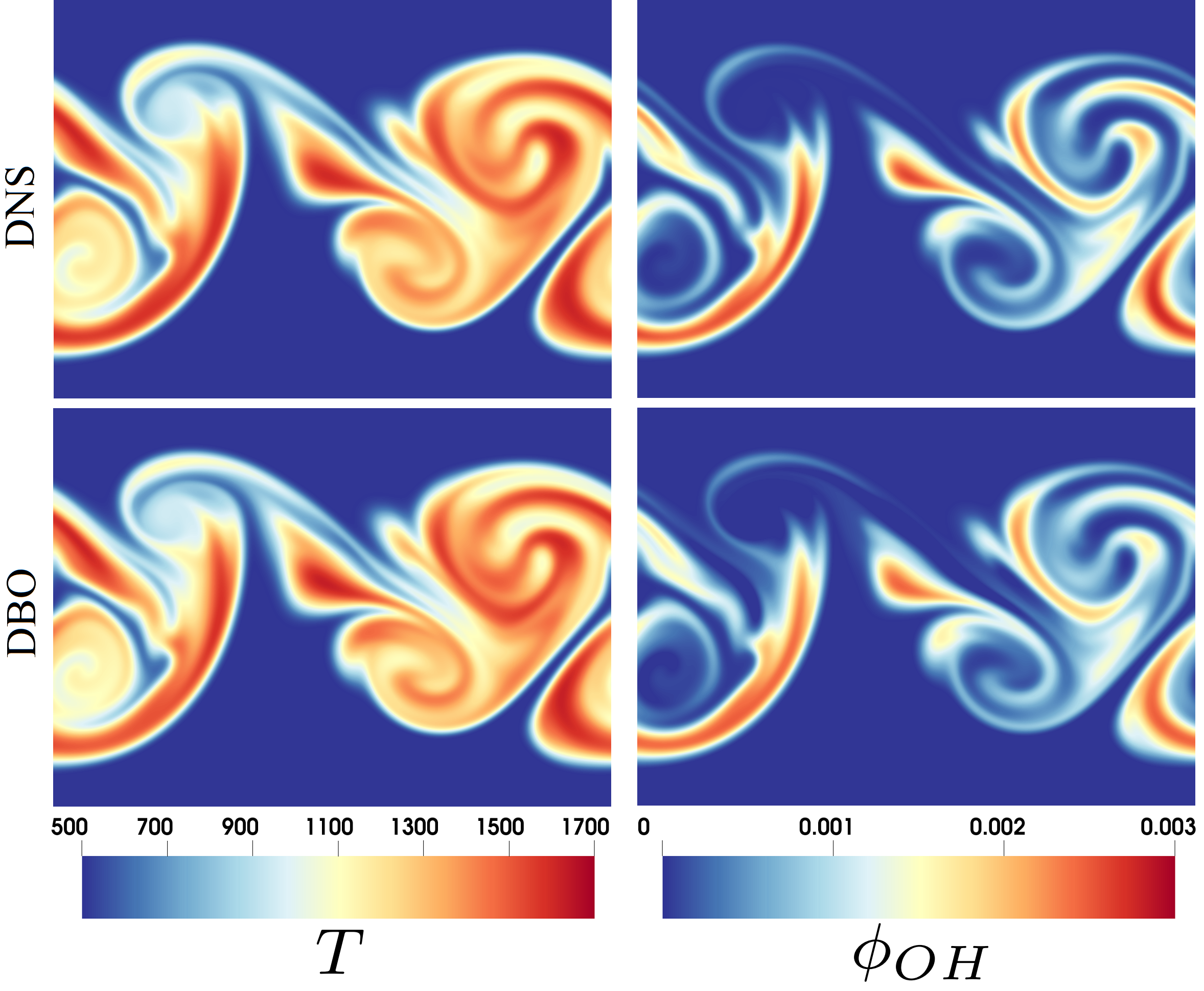
Fig. 3: Contour plots of the temperature ($T$) and the hydroxyl radical mass fraction ($\phi_{OH}$) fields at $t=30t_{j}$ obtained from DNS and DBO with $r=6$.

For a visual inspection, in Fig. 3, the temperature ($T$) and the mass fraction of the hydroxyl radical ($\phi_{OH}$) as obtained by DNS and DBO ($r=6$) are presented. The agreement is very good. Figure 4(a) provides the comparison between singular values obtained from I-PCA, i.e., the optimal reduction and those obtained from DBO with ranks $r=6$ and $r=8$. For both cases the leading singular values are captured very well. However, there is an error in capturing the lowest singular values due to the effects of the unresolved subspace. This error can be reduced by increasing the reduction rank $r$ as shown in Fig. 4(b).

For a comparative assessment of the compositional structure of the flame, representative manifolds encompassed by O₂-OH-Z, and temperature are presented in Fig.  5. This figure corroborates the agreements observed via visual inspections of the flowfield. Comparisons are also made of various statistics of the reactive trasnport ariables. The joint probability density functions (PDFs) of $Z$ and $\phi_{OH}$ ($P\left(\psi_{Z},\psi_{OH}\right)$) are generated by data sampled over the entire domain and are presented in Fig. 6. Here $\psi_{Q}$ denotes the sample space of scalar $Q$. The agreement between DBO approximation and DNS data are very good and, as expected, improves as $r$ increases. These PDFs are very similar to those attained in previous three-dimensional DNS of the same fuel [52].

To highlight the non-equilibrium character of the flame, the averaged temperature values, conditioned on the instantaneous mixture fraction $\overline{T|Z=\psi_{Z}}$ are shown in Fig. 7. Here, the overbar denotes the volume averaging and the vertical bar denotes the conditional statistics. The trends portrayed in this figure are identical to those in previous DNS [52] exhibiting initial flame extinction and its subsequent re-ignition. The excellent agreements between DBO and DNS is simply due to the fact that bases $U$ and $Y$ adapt to the physics for the conditions (in this case extinction and re-ignition). The higher the $r$ value is, the more details DBO resolves and more of the physics is captured.

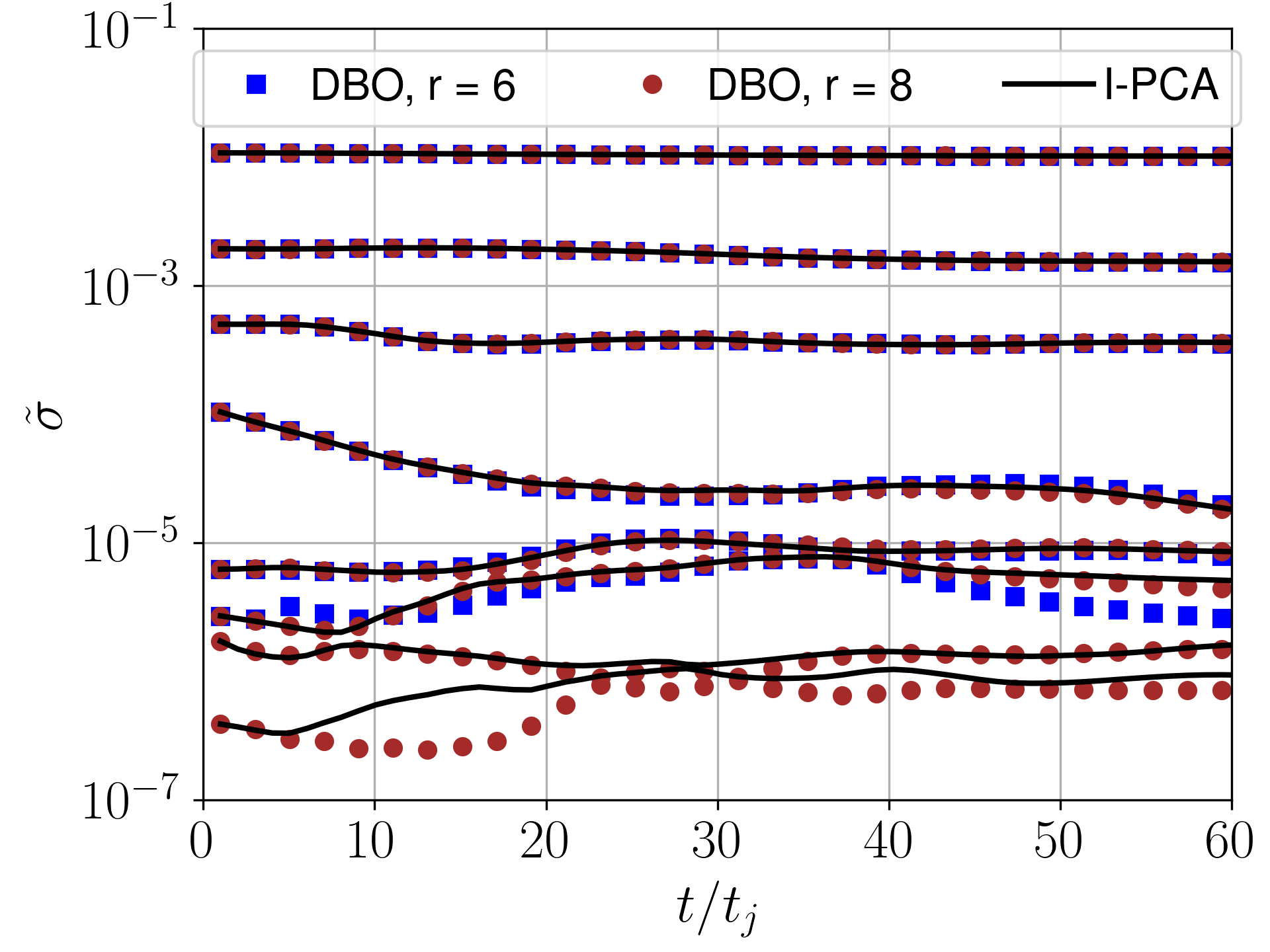
(a)

(b)

Fig. 4: Temporal evolution of (a) singular values and (b) Frobenius error in DBO.

Fig. 5: 3D manifolds of mixture fraction ($Z$), mass fractions of oxygen ($\phi_{O_{2}}$) and hydroxyl radical ($\phi_{OH}\times 100$) colored by temperature ($T$) at $t=40t_{j}$.

Fig. 6: Joint PDFs of mixture fraction and hydroxyl radical, $P\left(\psi_{Z},\psi_{OH}\right)$.

Fig. 7: Conditionally averaged temperature values.

5 Conclusions

An assessment is made of the performance of a recently developed dynamically bi-orthogonal (DBO) reduced-order modeling of turbulent combustion [43]. The DBO decomposition is an on-the-fly ROM technique with two distinguishing characteristics in comparison to PCA-based ROMs: (i) in DBO, the low-rank composition subspace is time-dependent as opposed to static; and (ii) no offline data generation is required in DBO and closed-form evolution equations for the low-rank subspaces are derived. The performance of the DBO approximation is assessed via simulations of a non-premixed CO/H₂ flame in a temporally evolving jet. The GRI-Mech 3.0 model with 53 species is used to model the chemical kinetics. This flame exhibits strong non-equilibrium effects including extinction and subsequent re-ignition. The simulated results clearly indicates that DBO yields excellent predictions of various statistics of the thermo-chemical variables. This warrants future implementation of DBO for simulation of complex turbulent combustion systems [61].

Acknowledgments

This work is sponsored by the National Science Foundation (NSF), USA under Grant CBET-2042918, and by the Air Force Office of Scientific Research award (PM: Dr. Fariba Fahroo) FA9550-21-1-0247. Computational resources are provided by the Center for Research Computing (CRC) at the University of Pittsburgh.

References

- [1] R. Bilger, S. Pope, K. Bray, J. Driscoll, Paradigms in turbulent combustion research, Proc. Combust. Inst. 30 (1) (2005) 21–42.
- [2] S. B. Pope, Small scales, many species and the manifold challenges of turbulent combustion, Proc. Combust. Inst. 34 (1) (2013) 1 – 31.
- [3] V. Raman, M. Hassanaly, Emerging trends in numerical simulations of combustion systems, Proc. Combust. Inst. 37 (2) (2019) 2073–2089.
- [4] T. Lu, C. Law, Toward accommodating realistic fuel chemistry in large-scale computations, Prog. Energy Combust. Sci. 35 (2) (2009) 192–215.
- [5] C. K. Westbrook, Y. Mizobuchi, T. J. Poinsot, P. J. Smith, J. Warnatz, Computational combustion, Proc. Combust. Inst. 30 (1) (2005) 125–157.
- [6] J. H. Chen, Petascale direct numerical simulation of turbulent combustion – fundamental insights toward predictive models, Proc. Combust. Inst. 33 (1) (2011) 99–123.
- [7] A. G. Nouri, P. Givi, D. Livescu, Modeling and simulation of turbulent nuclear flames in Type Ia supernovae, Prog. Aerosp. Sci. 108 (2019) 156–179.
- [8] P. A. Libby, F. A. Williams (Eds.), Turbulent Reacting Flows, Academic Press, London, UK, 1994.
- [9] W. R. Hawthorne, D. S. Wedell, H. C. Hottel, Mixing and combustion in turbulent gas jets, in: 3rd Symp. on Combustion, Flames and Explosion Phenomena, The Combustion Institute, Pittsburgh, PA, 1949, pp. 266–288.
- [10] H. L. Toor, Mass transfer in dilute turbulent and non-turbulent systems with rapid irreversible reactions and equal diffusivities, AIChE J. 8 (1) (1962) 70–78.
- [11] P. A. Libby, F. A. Williams (Eds.), Turbulent Reacting Flows, Vol. 44 of Topics in Applied Physics, Springer-Verlag, Heidelberg, 1980.
- [12] N. Peters, Laminar diffusion flamelet models in non-premixed turbulent combustion, Prog. Energ. Combust. 10 (3) (1984) 319–339.
- [13] R. S. Miller, C. K. Madnia, P. Givi, Structure of a turbulent reacting mixing layer, Combust. Sci. Technol. 99 (1994) 1–36.
- [14] S. M. de Bruyn Kops, J. J. Riley, G. Kosály, A. W. Cook, Investigation of modeling for non-premixed turbulent combustion, Flow Turbul. Combust. 60 (1) (1998) 105–122.
- [15] H. Pitsch, H. Steiner, Large-eddy simulation of a turbulent piloted methane/air diffusion flame (Sandia Flame D), Phys. Fluids 12 (10) (2000) 2541–2554.
- [16] M. Muradoglu, K. Liu, S. B. Pope, PDF modeling of a bluff-body stabilized turbulent flame, Combust. Flame 132 (1–2) (2003) 115–137.
- [17] H. Pitsch, Large-eddy simulation of turbulent combustion, Annu. Rev. Fluid Mech. 38 (2006) 453–482.
- [18] T. G. Drozda, M. R. H. Sheikhi, C. K. Madnia, P. Givi, Developments in formulation and application of the filtered density function, Flow Turbul. Combust. 78 (1) (2007) 35–67.
- [19] M. Ihme, H. Pitsch, Modeling of radiation and nitric oxide formation in turbulent nonpremixed flames using a flamelet/progress variable formulation, Phys. Fluids 20 (5) (2008) 055110–20.
- [20] M. B. Nik, S. L. Yilmaz, P. Givi, M. R. H. Sheikhi, S. B. Pope, Simulation of Sandia Flame D using velocity-scalar filtered density function, AIAA J. 48 (7) (2010) 1513–1522.
- [21] K. Bray, Laminar flamelets in turbulent combustion modeling, Combust. Sci. Technol. 188 (9) (2016) 1372–1375.
- [22] J. van Oijen, A. Donini, R. Bastiaans, J. ten Thije Boonkkamp, L. de Goey, State-of-the-art in premixed combustion modeling using flamelet generated manifolds, Prog. Energy Combust. Sci. 57 (2016) 30–74.
- [23] P. Trisjono, K. Kleinheinz, E. Hawkes, H. Pitsch, Modeling turbulence–chemistry interaction in lean premixed hydrogen flames with a strained flamelet model, Combust. Flame 174 (2016) 194–207.
- [24] N. Peters, Turbulent Combustion, Cambridge University Press, Cambridge, UK, 2000.
- [25] J. Sutherland, A. Parente, Combustion modeling using principal component analysis, Proc. Combust. Inst. 32 (1) (2009) 1563–1570.
- [26] O. Owoyele, T. Echekki, Toward computationally efficient combustion DNS with complex fuels via principal component transport, Combust. Theory Model 21 (4) (2017) 770–798.
- [27] L. van der Maaten, E. O. Postma, H. J. van den Herik, Dimensionality reduction: A comparative review, Published online (2007).
- [28] P. G. Constantine, Active Subspaces: Emerging Ideas for Dimension Reduction in Parameter Studies, SIAM, USA, 2015.
- [29] R. Vidal, Y. Ma, S. Sastry, Generalized principal component analysis (GPCA), IEEE T. Pattern Anal. 27 (12) (2005) 1945–1959.
- [30] J. Cardoso, Blind signal separation: Statistical principles, P. IEEE 86 (10) (1998) 2009–2025.
- [31] B. Schölkopf, A. Smola, K.-R. Müller, Nonlinear component analysis as a kernel eigenvalue problem, Neural Comput. 10 (5) (1998) 1299–1319.
- [32] N. D. Lawrence, Gaussian process latent variable models for visualisation of high dimensional data, in: Proceedings of the 16th International Conference on Neural Information Processing Systems, NIPS’03, MIT Press, Cambridge, MA, USA, 2003, pp. 329––336.
- [33] J. B. Tenenbaum, V. de Silva, J. C. Langford, A global geometric framework for nonlinear dimensionality reduction, Science 290 (5500) (2000) 2319–2323.
- [34] S. T. Roweis, L. K. Saul, Nonlinear dimensionality reduction by locally linear embedding, Science 290 (5500) (2000) 2323–2326.
- [35] S. Lafon, A. Lee, Diffusion maps and coarse-graining: A unified framework for dimensionality reduction, graph partitioning, and data set parameterization, IEEE T. Pattern Anal. 28 (9) (2006) 1393–1403.
- [36] J. N. Kutz, S. L. Brunton, B. W. Brunton, J. L. Proctor, Dynamic Mode Decomposition, SIAM, Philadelphia, PA, 2016.
- [37] K. Taira, S. L. Brunton, S. T. M. Dawson, C. W. Rowley, T. Colonius, B. J. McKeon, O. T. Schmidt, S. Gordeyev, V. Theofilis, L. S. Ukeiley, Modal analysis of fluid flows: An overview, AIAA J. 55 (12) (2017) 4013–4041.
- [38] T. P. Sapsis, P. F. Lermusiaux, Dynamically orthogonal field equations for continuous stochastic dynamical systems, Physica D 238 (23) (2009) 2347–2360.
- [39] H. Babaee, M. Choi, T. P. Sapsis, G. E. Karniadakis, A robust bi-orthogonal/dynamically-orthogonal method using the covariance pseudo-inverse with application to stochastic flow problems, J. Comput. Phys. 344 (2017) 303–319.
- [40] H. Babaee, An observation-driven time-dependent basis for a reduced description of transient stochastic systems, P. Roy. Soc. A 475 (2231) (2019) 20190506.
- [41] M. Cheng, T. Y. Hou, Z. Zhang, A dynamically bi-orthogonal method for time-dependent stochastic partial differential equations I: Derivation and algorithms, J. Comput. Phys. 242 (2013) 843–868.
- [42] P. Patil, H. Babaee, Real-time reduced-order modeling of stochastic partial differential equations via time-dependent subspaces, J. Comput. Phys. 415 (2020) 109511.
- [43] D. Ramezanian, A. G. Nouri, H. Babaee, On-the-fly reduced order modeling of passive and reactive species via time-dependent manifolds, Comput. Methods Appl. Mech. Eng. 382 (2021) 113882.
- [44] H. Babaee, T. P. Sapsis, A minimization principle for the description of modes associated with finite-time instabilities, P. Roy. Soc. A 472 (2186) (2016) 20150779.
- [45] A. G. Nouri, H. Babaee, P. Givi, H. Chelliah, D. Livescu, Skeletal model reduction with forced optimally time dependent modes, Combust. Flame 235 (2022) 111684.
- [46] M. Choi, T. P. Sapsis, G. E. Karniadakis, On the equivalence of dynamically orthogonal and bi-orthogonal methods: Theory and numerical simulations, J. Comput. Phys. 270 (2014) 1–20.
- [47] E. Musharbash, F. Nobile, T. Zhou, Error analysis of the dynamically orthogonal approximation of time dependent random PDEs, SIAM J. Sci. Comput. 37 (2) (2015) A776–A810.
- [48] H. Babaee, M. Farazmand, G. Haller, T. Sapsis, Reduced-order description of transient instabilities and computation of finite-time Lyapunov exponents, Chaos 27 (6) (2017) 063103.
- [49] M. Beck, A. Jäckle, G. Worth, H.-D. Meyer, The multiconfiguration time-dependent hartree (MCTDH) method: A highly efficient algorithm for propagating wavepackets, Phys. Rep. 324 (1) (2000) 1–105.
- [50] O. Koch, C. Lubich, Dynamical low-rank approximation, SIAM J. Matrix Anal. A. 29 (2) (2007) 434–454.
- [51] A. Aitzhan, S. Sammak, P. Givi, A. G. Nouri, PeleLM-FDF large eddy simulator of turbulent combustion, arXiv preprint arXiv:2201.00898 (2022).
- [52] E. R. Hawkes, R. Sankaran, J. C. Sutherland, J. H. Chen, Scalar mixing in direct numerical simulations of temporally evolving plane jet flames with skeletal CO/H2 kinetics, Proc. Combust. Inst. 31 (1) (2007) 1633–1640.
- [53] Y. Yang, H. Wang, S. B. Pope, J. H. Chen, Large-eddy simulation/probability density function modeling of a non-premixed CO/H2 temporally evolving jet flame, Proc. Combust. Inst. 34 (1) (2013) 1241–1249.
- [54] N. Punati, J. C. Sutherland, A. R. Kerstein, E. R. Hawkes, J. H. Chen, An evaluation of the one-dimensional turbulence model: Comparison with direct numerical simulations of CO/H2 jets with extinction and reignition, Proc. Combust. Inst. 33 (1) (2011) 1515–1522.
- [55] S. Vo, A. Kronenburg, O. T. Stein, M. J. Cleary, MMC-LES of a syngas mixing layer using an anisotropic mixing time scale model, Combust. Flame 189 (2018) 311–314.
- [56] S. Yang, R. Ranjan, V. Yang, W. Sun, S. Menon, Sensitivity of predictions to chemical kinetics models in a temporally evolving turbulent non-premixed flame, Combust. Flame 183 (2017) 224–241.
- [57] B. A. Sen, E. R. Hawkes, S. Menon, Large eddy simulation of extinction and reignition with artificial neural networks based chemical kinetics, Combust. Flame 157 (3) (2010) 566–578.
- [58] G. P. Smith, D. M. Golden, M. Frenklach, N. W. Moriarty, B. Eiteneer, M. Goldenberg, C. T. Bowman, R. K. Hanson, S. Song, W. C. Gardiner, Jr., V. V. Lissianski, Z. Qin, GRI-Mech home page, available at http://combustion.berkeley.edu/gri-mech/, (last accessed: 12-31-2021) (1999).
- [59] A. Nonaka, M. S. Day, J. B. Bell, A conservative, thermodynamically consistent numerical approach for low Mach number combustion. Part I: Single-level integration, Combust. Theor. Model. 22 (1) (2018) 156–184.
- [60] R. W. Bilger, The structure of diffusion flames, Combust. Sci. Technol. 13 (1-6) (1976) 155–170.
- [61] L. Y. M. Gicquel, G. Staffelbach, T. Poinsot, Large eddy simulation of gaseous flames in gas turbine combustion chambers, Prog. Energ. Combust. 38 (6) (2012) 782–817.