Asymptotic Behavior of Inter-Event Times in Planar Systems under Event-Triggered Control

Abstract

This paper analyzes the asymptotic behavior of inter-event times in planar linear systems, under event-triggered control with a general class of scale-invariant event triggering rules. In this setting, the inter-event time is a function of the “angle” of the state at an event. This viewpoint allows us to analyze the inter-event times by studying the fixed points of the “angle” map, which represents the evolution of the “angle” of the state from one event to the next. We provide a sufficient condition for the convergence or non-convergence of inter-event times to a steady state value under a scale-invariant event-triggering rule. Following up on this, we further analyze the inter-event time behavior in the special case of threshold based event-triggering rule and we provide various conditions for convergence or non-convergence of inter-event times to a constant. We also analyze the asymptotic average inter-event time as a function of the angle of the initial state of the system. With the help of ergodic theory, we provide a sufficient condition for the asymptotic average inter-event time to be a constant for all non-zero initial states of the system. Then, we consider a special case where the “angle” map is an orientation-preserving homeomorphism. Using rotation theory, we comment on the asymptotic behavior of the inter-event times, including on whether the inter-event times converge to a periodic sequence. We illustrate the proposed results through numerical simulations.

1 Introduction

Event-triggered control is commonly used in several applications with resource constraints. Efficiency of this control method is due to the state dependent and non-constant inter-event times, which are implicitly determined by a state-dependent event-triggering rule. However, this also means that the evolution of the inter-event times is difficult to predict, which makes higher level planning and scheduling difficult. Further, there is not enough work that analytically quantifies the improvement in resource usage by event-triggered controllers compared to time-triggered controllers. From both these points of view, it is very useful to analyze the inter-event times generated by event-triggered controllers. With these motivations, in this paper, we carry out a systematic analysis of the asymptotic behavior of inter-event times for planar linear systems under a general class of scale-invariant event-triggering rules.

1.1 Literature review

Event-triggered control is a popular control method in the field of networked control systems [1, 2, 3, 4]. In the literature on this topic, inter-event time analysis is typically limited to showing the existence of a positive lower bound on the inter-event times to guarantee the absence of zeno behavior. Among the exceptions to this rule, a few works provide bounds on the average sampling rate [5, 6, 7]. References [8, 9] consider a scalar stochastic event-triggered control system and provide a closed form expression for the expected average sampling period or communication rate. There are also some works [10, 11, 12, 13] that determine the necessary and sufficient data rates for achieving the control objective irrespective of the controller that is used. References [14, 15] take a different point of view and design event triggering rules that guarantee better performance than periodic time-triggered control, for a given average sampling rate. Reference [16] designs an event-triggered controller that ensures exponential stability of the closed loop system while satisfying some given interval constraints on event times. Whereas, self-triggered [17] and periodic event triggered [18] control methods guarantee the absence of zeno behavior by design.

Evolution of inter-event times is far less studied topic in the literature. We believe reference [19] is the first paper to analyze the periodic and chaotic patterns exhibited by the inter-event sequences of linear time invariant systems under homogeneous event-triggering rules. Reference [20] analyzes the evolution of inter-event times for planar linear systems under time-regularized relative thresholding event-triggering rule. Specifically, this paper explains the commonly observed behaviors of inter-event times, such as steady-state convergence and oscillatory nature, under the “small” thresholding parameter and “small” time-regularization parameter scenario. However, these results are qualitative in nature as they do not clearly specify the bounds on the parameters for which the claims hold. At the same time,  [20] does not provide explicit bounds on the behavior of inter-event times. Reference [21] takes a different approach to characterize the sampling behavior of linear time-invariant event-triggered control systems by using finite-state abstractions of the system. The same idea is extended to nonlinear and stochastic event-triggered control systems by references [22] and [23], respectively. On the other hand, [24] provides a framework to estimate the smallest, over all initial states, average inter-sample time of a linear periodic event-triggered control system by using finite-state abstractions. Reference [25] improves the above approach by showing robustness to small enough model uncertainties. The paper [26] shows that the abstraction based method can also be used to analyze the chaotic behavior exhibited by the traffic patterns of periodic event-triggered control systems.

Our previous work [27] analyzes the evolution of inter-event times for planar linear systems under a general class of event-triggering rules. This work is a continuation of the same. In one of our recent works [28], we analyze the inter-event time evolution in linear systems under region-based self-triggered control. In this control method, the state space is partitioned into a finite number of conic regions and each region is associated with a fixed inter-event time.

1.2 Contributions

The major contribution of our work is that we analyze the asymptotic behavior of the inter-event times, such as convergence to a constant or to a periodic sequence, in planar linear systems under a general class of scale-invariant event-triggering rules. We carry out this analysis by essentially studying how the “angle” of the state evolves from one event to the next. We also leverage the literature on ergodic theory and rotation theory in our analysis. Under mild technical assumptions, we catalogue the different kinds of asymptotic behavior of the “angle” of the state and as a consequence the asymptotic behavior of the inter-event times. We also analyze the asymptotic average inter-event time as a function of the “angle” of the initial state of the system. Our results are quantitative in nature and are applicable for a very broad class of event-triggering rules. We next provide an overview of the contributions of our paper relative to closely related works from the literature.

While [19] seeks to study the evolution of inter-event times by understanding the state evolution, the results in the paper are quite preliminary. In the current paper, we provide several necessary conditions and sufficient conditions on the system parameters which could be used to predict convergence or lack of convergence of inter-event times to a constant. The results in [20] are restricted to planar linear systems under time-regularized relative thresholding based event-triggering in the “small relative threshold parameter and time-regularization parameter” setting. [20] does not explicitly mention the bounds on these parameters for which the results hold, nor is the derivation of such bounds obvious from the analysis. In contrast, our results hold for all range of parameters. In fact, aided by one of our analytical results, we show through simulations that the analytical results and interpretations in [20] are not necessarily true for large enough parameters. Further,  [19, 20] analyze specific triggering rules, whereas our results hold for a general class of scale invariant rules. References [21, 22, 23, 24, 25, 26] characterize the sampling behavior of event-triggered control systems by using finite state-space abstractions of the system. However, this approach can be computationally very demanding.

The main contributions of this paper with respect to our previous work [27] are stability analysis of the fixed points of the “angle” map under any scale-invariant quadratic event-triggering rule and a framework to analyze the asymptotic average inter-event time as a function of the initial state of the system. We also provide several important new results and improve some of the existing results. We also improve the numerical examples section by including more simulation results.

1.3 Organization

Section 2 formally sets up the problem and states the objective of this paper. Section 3 and Section 4 analyze the properties of the inter-event time as a function of the state at an event and the steady-state behavior of inter-event times under the event-triggered control method, respectively. In Section 5, with the help of ergodic theory and rotation theory, we study the asymptotic average inter-event time as a function of the initial state of the system. Section 6 illustrates the results using numerical examples. Finally, we provide some concluding remarks in Section 7.

1.4 Notation

Let , $\mathbb{R}_{\geq 0}$, and $\mathbb{R}_{>0}$ denote the set of all real, non-negative real and positive real numbers, respectively. $\mathbb{R}\setminus\{0\}$ and $\mathbb{R}^{n}\setminus\{0\}$ denote the set of all non-zero real numbers and the set of all non-zero vectors in ⁿ, respectively. Let ${\mathbb{N}}$ and ${\mathbb{N}}_{0}$ denote the set of all positive and non-negative integers, respectively. For any $x\in^{n}$, $\left\lVert x\right\rVert$ denotes the euclidean norm of $x$. For an $n\times n$ square matrix $A$, let $\det(A)$ and $\mathrm{tr}(A)$ denote determinant and trace of $A$, respectively. $B_{\epsilon}(u):=\{x\in^{n}:\left\lVert x-u\right\rVert\leq\epsilon\}$ represents an $n-$dimensional ball of radius $\epsilon$ centered at $u\in^{n}$. Let $(X,\mathcal{B},\mu)$ be a measure space where $X$ is a set, $\mathcal{B}=\mathcal{B}(X)$ is the borel $\sigma-$algebra on the set $X$ and $\mu$ is a measure on the measurable space $(X,\mathcal{B})$.

2 Problem Setup

In this section, we formulate the problem of analyzing the asymptotic behavior of inter-event times in event-triggered control systems. We begin by specifying the class of systems and event-triggering rules that we consider and then state the main objective of this paper.

2.1 System Dynamics

Consider a linear time invariant planar system,

$$\dot{x}(t)=Ax(t)+Bu(t),$$ (1a)

where $$x\in^{2} u\in^{m} A\in^{2\times 2} B\in^{2\times m} \{t_{k}\}_{k\in{\mathbb{N}}_{0}}$$ is the plant state and is the control input, while and are the system matrices. Consider a sampled data controller and let be the sequence of event times at which the state is sampled and the control input is updated as follows,

$$u(t)=Kx(t_{k}),\quad\forall t\in[t_{k},t_{k+1}).$$ (1b)

Let the control gain $K$ be such that $A_{c}:=A+BK$ is Hurwitz.

2.2 Triggering Rules

In this paper, we assume that the event times $\{t_{k}\}_{k\in{\mathbb{N}}_{0}}$ are generated in an event-triggered manner so as to implicitly guarantee asymptotic stability of the origin of the closed loop system. It is common to construct such event-triggering rules based on a candidate Lyapunov function. For example, consider a quadratic candidate Lyapunov function $V(x)=x^{T}Px$, where $P\in^{2\times 2}$ is a positive definite symmetric matrix that satisfies the Lyapunov equation

$$PA_{c}+A_{c}^{T}P=-Q,$$ (2)

for a given symmetric positive definite matrix $Q$. Following are three different event-triggering rules that are commonly used in the literature for stabilization tasks.

$$t_{k+1} =\min\{t>t_{k}:\dot{V}(x(t))=0\}$$ (3a)

$$t_{k+1} =\min\{t>t_{k}:\left\lVert x(t_{k})-x(t)\right\rVert=\sigma\left\lVert x(t)\right\rVert\},$$ (3b)

$$t_{k+1} =\min\{t>t_{k}:V(x(t))=V(x(t_{k}))e^{-r(t-t_{k})}\}.$$ (3c)

First two triggering rules render the origin of the closed loop system asymptotically stable, with $\sigma$ sufficiently small in the latter rule. The third event-triggering rule ensures exponential stability for a sufficiently small $r>0$.

During the inter-event intervals, we can write the solution $x(t)$ of system (1) as

$$x(t)=G(\tau)x(t_{k}),\quad\forall t\in[t_{k},t_{k+1}),$$

where $\tau:=t-t_{k}$ and

$$G(\tau):=\mathrm{e}^{A\tau}+\int_{0}^{\tau}\mathrm{e}^{A(\tau-s)}\mathrm{d}s(A_{c}-A).$$

Using this structure of the solution, we can write the three triggering rules (3) as

$$t_{k+1}-t_{k}=\min\{\tau>0:f(x(t_{k}),\tau):=x^{T}(t_{k})M(\tau)x(t_{k})=0\},$$ (4)

where $M(\tau)$ is a time varying symmetric matrix. In particular, for the triggering rules (3a)-(3c) $M(\tau)$ is equal to $M_{1}(\tau)$, $M_{2}(\tau)$ and $M_{3}(\tau)$, respectively, where

$$M_{1}(\tau) :=\frac{\mathrm{d}G^{T}(\tau)}{\mathrm{d}\tau}PG(\tau)+G^{T}(\tau)P\frac{\mathrm{d}G(\tau)}{\mathrm{d}\tau}$$ (5a)

$$M_{2}(\tau) :=(1-\sigma^{2})G^{T}(\tau)G(\tau)-(G^{T}(\tau)+G(\tau))+I$$ (5b)

$$M_{3}(\tau) :=G^{T}(\tau)PG(\tau)-P\mathrm{e}^{-r\tau}.$$ (5c)

Note that if $A$ is invertible, then the expression and computation of $M(\tau)$ is simplified significantly as

$$G(\tau)=I+A^{-1}(\mathrm{e}^{A\tau}-I)A_{c}.$$

2.3 Objective

The main objective of this paper is to analyze the evolution of inter-event times along the trajectories of system (1) for the general class of event triggering rules (4). We seek to provide analytical guarantees for the asymptotic behavior of inter-event times under these rules. Specifically, we would like to answer the questions: when do the inter-event times converge to a steady-state value or to a periodic sequence and when do the asymptotic average inter-event times becomes a constant for all initial states of the system. We also want to analyze the asymptotic average inter-event time as a function of the initial state of the system. The approach we take is to analyze inter-event time and the state at the next event as functions of the state at the time of the current event.

3 Inter-event time as a function of the state

In this section, we analyze the inter-event time $t_{k+1}-t_{k}$, as a function of $x(t_{k})$, for the system (1) under the general class of event triggering rules (4). Formally, we define the inter-event time function $\tau_{e}:\mathbb{R}^{2}\setminus\{0\}\rightarrow\mathbb{R}_{>0}$ as

$$\tau_{e}(x):=\min\{\tau>0:f(x,\tau)=x^{T}M(\tau)x=0\}.$$ (6)

We can write $t_{k+1}-t_{k}=\tau_{e}(x(t_{k}))$ for all $k\in{\mathbb{N}}_{0}$. Next, we analyze the properties of this inter-event time function such as scale-invariance, periodicity and continuity.

3.1 Properties of the inter-event time function

Remark 1.

(The inter-event time function is scale-invariant). Note from (6) that $f(\alpha x,\tau)=\alpha^{2}f(x,\tau)$ for all $\alpha\in$ and $x\in^{2}$. Hence, $\tau_{e}(\alpha x)=\tau_{e}(x)$, for any $x\in\mathbb{R}^{2}\setminus\{0\}$ and for any $\alpha\in\mathbb{R}\setminus\{0\}$. $\bullet$

The scale-invariance property implies that we can redefine the inter-event time function for planar systems as a scalar function $\tau_{s}:\rightarrow\mathbb{R}_{>0}$,

$$\tau_{s}(\theta):=\min\{\tau>0:f_{s}(\theta,\tau):=x_{\theta}^{T}M(\tau)x_{\theta}=0\},$$ (7)

where $x_{\theta}:=\begin{bmatrix}\cos(\theta)&\sin(\theta)\end{bmatrix}^{T}$, so that $\tau_{e}(x)=\tau_{s}(\theta)$ for $x=\alpha x_{\theta}$ for all $\alpha\in\mathbb{R}\setminus\{0\}$. Hence for a planar system, the inter-event time $t_{k+1}-t_{k}=\tau_{s}(\theta_{k})$ for all $k\in{\mathbb{N}}_{0}$, where $\theta_{k}$ is the angle between $x(t_{k})$ and the $x_{1}$ axis.

Remark 2.

($\tau_{s}(\theta)$ is a periodic function with period $\pi$). We know that for
$x_{\theta}=\begin{bmatrix}\cos(\theta)&\sin(\theta)\end{bmatrix}^{T}$, $\tau_{s}(\theta)=\tau_{e}(x_{\theta})=\tau_{e}(-x_{\theta})=\tau_{s}(\theta+\pi)$ for all $\theta\in$. $\bullet$

Periodicity of $\tau_{s}(\theta)$ helps us to restrict our analysis to the domain $[0,\pi)$. Next, we present an important property of $f_{s}(\theta,\tau)$ that plays a major role in the subsequent analysis.

Lemma 3.

(For any fixed $\tau$, $f_{s}(\theta,\tau)$ is a sinusoidal function with a shift in phase and mean). Let $m_{ij}(\tau)$ be the $(ij)^{th}$ element of $M(\tau)\in^{2\times 2}$. For any fixed $\tau\in\mathbb{R}_{>0}$,

$$f_{s}(\theta,\tau)=\frac{\mathrm{tr}(M(\tau))}{2}+a\sin\left(2\theta+\arctan\left(b\right)\right),$$ (8)

$$a:=\frac{1}{2}\sqrt{(\mathrm{tr}(M(\tau)))^{2}-4\det(M(\tau))},\ b:=\frac{m_{11}(\tau)-m_{22}(\tau)}{2m_{12}(\tau)}.$$

Proof.

Here, we skip the time argument of $m_{ij}(\tau)$ for brevity. Note that $m_{12}=m_{21}$. Then, for any fixed $\tau\in\mathbb{R}_{>0}$,

$$f_{s}(\theta,\tau) =\begin{bmatrix}\cos(\theta)&\sin(\theta)\end{bmatrix}M(\tau)\begin{bmatrix}\cos(\theta)\\ \sin(\theta)\end{bmatrix},$$ (9)

$$=m_{11}\cos^{2}(\theta)+m_{22}\sin^{2}(\theta)+2m_{12}\cos(\theta)\sin(\theta),$$

$$=m_{11}+(m_{22}-m_{11})\sin^{2}(\theta)+m_{12}\sin(2\theta),$$

$$=\frac{m_{11}+m_{22}}{2}+\frac{m_{11}-m_{22}}{2}\cos(2\theta)+m_{12}\sin(2\theta),$$

which when suitably re-expressed gives the result. ∎

Using the structure of $f_{s}(\theta,\tau)$ in (8) and the quadratic form (9), we can easily determine the number of solutions to $f_{s}(\theta,\tau)=0$ for any fixed $\tau$.

Corollary 4.

(Number of solutions $\theta$ to $f_{s}(\theta,\tau)=0$ for a fixed $\tau$). For any fixed $\tau\in\mathbb{R}_{>0}$, if $\det(M(\tau))>0$, then $f_{s}(\theta,\tau)=0$ has no solutions; if $\det(M(\tau))=0$ then $f_{s}(\theta,\tau)=0$ has a single solution $\theta\in[0,\pi)$ or $f_{s}(\theta,\tau)=0$ for all $\theta\in[0,\pi)$; if $\det(M(\tau))<0$ then $f_{s}(\theta,\tau)=0$ has exactly two solutions $\theta\in[0,\pi)$. ∎

From the quadratic form (9), we can also obtain a necessary and sufficient condition for the event-triggering rule (4) to reduce to a periodic triggering rule, with inter-event times that are independent of the state.

Corollary 5.

(Necessary and sufficient condition for the triggering rule (4) to reduce to periodic triggering). $\tau_{s}(\theta)=\tau_{1},\forall\theta\in[0,\pi)$ if and only if $\det(M(\tau))>0$ for all $\tau\in(0,\tau_{1})$, $\tau_{1}=\min\{\tau>0:\det(M(\tau))=0\}$ and $M(\tau_{1})=0$, the zero matrix. ∎

Note that this necessary and sufficient condition depends only on the time varying matrix $M(\tau)$, which can be determined given the system parameters and the event-triggering rule. If we know that the triggering rule for a given event-triggered control system is periodic, then further analysis of inter-event times is not required.

3.2 Continuity of the inter-event time function $\tau_{s}(\theta)$

In this subsection, we seek to obtain conditions under which the inter-event time function $\tau_{s}(\theta)$ is continuous. Towards this aim, we make the following assumption about the matrix function $M(\tau)$ since the general class of event-triggering rules (4) for an arbitrary $M(\tau)$ is very broad.

1. Every element of the matrix $M(.)$ is a real analytic function of $\tau$ and there exists a $\tau_{m}$ such that $M(\tau)$ is negative definite for $(0,\tau_{m})$, where

   $$\tau_{m}:=\min\{\tau>0:\det(M(\tau))=0\}.$$

It is easy to verify that each $M_{i}(.)$ in (5), corresponding to the three triggering rules (3), satisfies Assumption (A1). This is because in $M_{1}(.)$ and $M_{2}(.)$ the dependence on $\tau$ comes from the matrix exponential $\mathrm{e}^{A\tau}$ and its integral with respect to $\tau$. In $M_{3}(.)$, there is an additional exponential function $\mathrm{e}^{-r\tau}$ which is combined linearly with other terms dependent on $\tau$. Letting $J:=S^{-1}AS$ be the real Jordan form of $A$, we have $\mathrm{e}^{A\tau}=S\mathrm{e}^{J\tau}S^{-1}$. Thus, each element of $M_{i}(.)$ is a linear combination of products of exponential functions, polynomials (in case $A$ is not diagonalizable) and sinusoidal functions (in case $A$ has complex eigenvalues), all of which are real analytic functions of $\tau$. Thus, each of the $M_{i}(.)$’s are real analytic functions of $\tau$. Note that these arguments hold true even if $A$ is singular. Further, both $M_{1}(0)$ and $M_{2}(0)$ are negative definite. Though $M_{3}(0)=0$ the time derivative of $M_{3}$ at $\tau=0$, $\dot{M}_{3}(0)$, is negative definite for suitable $P$ and $r$.

Now, let $\tau_{\min}$ and $\tau_{\max}$ denote the global minimum and the global maximum of $\tau_{s}(\theta)$, respectively, that is,

$$\tau_{\min}:=\min_{\theta\in[0,\pi)}\tau_{s}(\theta),\quad\tau_{\max}:=\max_{\theta\in[0,\pi)}\tau_{s}(\theta).$$

For a matrix $M(.)$ that satisfies Assumption (A1), clearly $\tau_{\min}=\tau_{m}$ as $\det(M(\tau))>0$ in the interval $(0,\tau_{m})$ and according to Corollary 4, $f_{s}(\theta,\tau)=0$ has no solution for $\tau\in(0,\tau_{m})$ and has a solution for $\tau=\tau_{m}$. In general, $\tau_{\max}$ may not exist, that is $\tau_{\max}=\infty$. In this case, it means that there exists a $x_{0}\in\mathbb{R}^{2}\setminus\{0\}$ such that if $x(t_{k})=x_{0}$ then $t_{k+1}=\infty$. However, such an $x_{0}$ cannot exist if $A$ has positive real parts for both its eigenvalues and if the triggering rule (4) ensures $x=0$ is asymptotically stable. In such a case, $\tau_{\max}$ is a finite quantity.

We approach the question of continuity of the inter-event time function $\tau_{s}(\theta)$ by first analyzing the smoothness properties of the level set $f_{s}(\theta,\tau)=0$ in the $(\theta,\tau)$ space. In particular, Assumption (A1) implies that $\det(M(\tau))$ is also real analytic and as a result it has finitely many zeros in the interval $\tau\in[0,\tau_{\max}]$. This observation, along with Corollary 4, can be used to say that $f_{s}(\theta,\tau)=0$ has finitely many connected branches, which are arbitrarily smooth, in the set $\{(\theta,\tau)\in[0,\pi)\times[0,\tau_{\max}]\}$. We formally state this claim in the following result.

Lemma 6.

(The level set $f_{s}(\theta,\tau)=0$ has finitely many connected branches, which are arbitrarily smooth). Suppose that $M(.)$ in (7) satisfies Assumption (A1) and $\tau_{\max}<\infty$. Then, the level set $f_{s}(\theta,\tau)=0$ has finitely many connected branches in the set $\{(\theta,\tau)\in[0,\pi)\times[0,\tau_{\max}]\}$. Each branch is an arbitrarily smooth curve in $(\theta,\tau)$ space and can be parameterized by $\tau$ in a closed interval.

Proof.

First note that under Assumption (A1), all elements of $M(.)$ are real analytic functions, which implies that $\det(M(\tau))$ is also a real analytic function of $\tau$. This is true because the determinant of a matrix is a polynomial of its elements, and products and sums of real analytic functions are also real analytic. As a consequence, on the closed and bounded interval $[0,\tau_{\max}]$, $\det(M(\tau))$ has finitely many zeros. This implies that there are finitely many sub-intervals $[g_{i},h_{i}]$ of $[0,\tau_{\max}]$ such that $\det(M(g_{i}))=\det(M(h_{i}))=0$ and $\det(M(\tau))<0$ for all $\tau\in(g_{i},h_{i})$. Then, Corollary 4 guarantees that $f_{s}(\theta,\tau)=0$ has exactly two solutions for each $\tau\in[g_{i},h_{i}]$ for each of the finitely many $i$, with the two solutions coincident at $g_{i}$ and $h_{i}$ but nowhere else. Thus, $f_{s}(\theta,\tau)=0$ has finitely many branches in $\{(\theta,\tau)\in[0,\pi)\times[0,\tau_{\max}]\}$. Smoothness of the branches is a consequence of the fact that $f_{s}(\theta,\tau)$ is an arbitrarily smooth function, which is also evident from (8). ∎

Lemma 6 allows us to apply the implicit function theorem on $f_{s}(\theta,\tau)=0$ at all $(\theta,\tau_{s}(\theta))\in[0,\pi)\times[0,\tau_{\max}]$, except at finitely many points. From this, we guarantee that $\tau_{s}(\theta)$ is continuously differentiable in $[0,\pi)$, except at finitely many points.

Theorem 7.

(Inter-event time function is continuously differentiable except for finitely many $\theta$). Suppose that $M(.)$ in (7) satisfies Assumption (A1) and $\tau_{\max}<\infty$. Then, the inter-event time function $\tau_{s}(\theta)$, defined as in (7), is continuously differentiable on $[0,\pi)$ except at finitely many $\theta$.

Proof.

Recalling Lemma 6, consider any one of the finitely many branches of the level set $f_{s}(\theta,\tau)=0$ in the set $\{(\theta,\tau)\in[0,\pi)\times[0,\tau_{\max}]\}$. We denote the smooth parameterization of the branch by $\tau$ as $\theta(\tau)$. Then, by Theorem 1 in [29] (Morse-Sard Theorem for real analytic functions), we can say that the critical values $\theta$ of the function $\theta(\tau)$ form a finite set. We can infer two observations from this. First, in tracing out the $\tau_{s}(\theta)$ function, there are finitely many jumps between the branches of the level set $f_{s}(\theta,\tau)=0$ in the set $\{(\theta,\tau)\in[0,\pi)\times[0,\tau_{\max}]\}$. Second, for all $\theta\in[0,\pi)$ except at finitely many $\theta$, $\frac{\partial f_{s}(\theta,\tau)}{\partial\tau}|_{(\theta,\tau_{s}(\theta))}\neq 0$ and therefore the implicit function theorem guarantees continuous differentiability of $\tau_{s}(\theta)$ on $[0,\pi)$ except at finitely many $\theta$. ∎

Based on Theorem 7 and its proof, we provide a sufficient condition for $\tau_{s}(\theta)$ to be continuously differentiable.

Corollary 8.

(Corollary to Theorem 7). If $\frac{\partial f_{s}(\bar{\theta},\bar{\tau})}{\partial\tau}\neq 0$ for all $(\bar{\theta},\bar{\tau})\in\times$ such that $f_{s}(\bar{\theta},\bar{\tau})=0$, then the inter-event time function $\tau_{s}:\rightarrow\mathbb{R}_{>0}$ defined as in (7) is continuously differentiable. ∎

Since in simulations, we encounter $\tau_{s}(\theta)$ functions that visually seem to be continuous quite often, we present the following result in the special case where $\tau_{s}(\theta)$ is a continuous function.

Proposition 9.

If the inter-event time function $\tau_{s}(\theta)$ is a continuous function, then every local extremum of $\tau_{s}(\theta)$ is a global extremum.

Proof.

We prove this result by contradiction. Suppose there exists an extremum of $\tau_{s}(\theta)$ at $\theta_{1}$ with value $\tau_{1}\in(\tau_{\min},\tau_{\max})$. That is, the extremum at $\theta_{1}$ is not a global extremum. Then, the assumptions that $\tau_{s}(\theta)$ is continuous and $\theta_{1}$ is a local extremizer and the fact that $\tau_{s}(\theta)$ is periodic with period $\pi$ imply that there exist $\theta_{2},\theta_{3}\in(\theta_{1},\theta_{1}+\pi)$ such that $\tau_{s}(\theta_{2})=\tau_{s}(\theta_{3})=\tau_{s}(\theta_{1})=\tau_{1}$. However, this contradicts Corollary 4, which says that for any given $\tau_{1}>0$, $f_{s}(\theta,\tau_{1})=0$, and hence $\tau_{s}(\theta)=\tau_{1}$, can at most have two solutions for $\theta$. Therefore, the claim in the result must be true. ∎

4 Evolution of the inter-event time

In this section, we provide a framework for analyzing the evolution of the inter-event time along the trajectories of the system (1) under the general class of event-triggering rules (4). In the previous section we showed that, for scale-invariant event-triggering rules, the inter-event time is determined completely by the angle of the state at the current event-triggering instant. So, we restrict our analysis to the domain $R^{1}:=/2\pi{\mathbb{Z}}$, which is defined as the quotient of real numbers by the equivalence relation of differing by an integer multiple of $2\pi$. Then we define a map $\phi:R^{1}\to R^{1}$, referred to as “angle” map, which represents the evolution of the “angle” of the state from one event to the next as,

$$\theta_{k+1}=\phi(\theta_{k}):=\text{arg}\left(G(\tau_{s}(\theta_{k}))\begin{bmatrix}\cos(\theta_{k})\\ \sin(\theta_{k})\end{bmatrix}\right),$$ (10)

where

$$\text{arg}(x):=\begin{cases}\arctan(\frac{x_{2}}{x_{1}}),\ &\text{if }x_{1}>0,x_{2}\geq 0\\ \pi+\arctan(\frac{x_{2}}{x_{1}}),\ &\text{if }x_{1}<0\\ 2\pi+\arctan(\frac{x_{2}}{x_{1}}),\ &\text{if }x_{1}>0,x_{2}<0\\ \frac{\pi}{2},\ &\text{if }x_{1}=0,x_{2}>0\\ \frac{-\pi}{2},\ &\text{if }x_{1}=0,x_{2}<0\\ \text{undefined},\ &\text{if }x_{1}=0,x_{2}=0.\end{cases}$$

and $\theta_{k}=\text{arg}(x(t_{k}))$ denotes the angle between the state $x(t_{k})$ and the positive $x_{1}$ axis. Thus, analysis of the inter-event time function $\tau_{s}(\theta)$ and the “angle” map $\phi(\theta)$ helps us to understand the evolution of the inter-event time for an arbitrary initial condition $x(t_{0})$. In particular, the analysis of fixed points of the “angle” map helps us to determine the steady state behavior of the inter-event times. This is the main idea behind the following result.

Theorem 10.

(Sufficient condition for the convergence or non-convergence of inter-event times to a steady state value). Consider the planar system (1) along with the event-triggering rule (4), for a general $M(.)$ that satisfies Assumption (A1).

• Suppose there exists a fixed point of the “angle” map, i.e., $\exists\theta$ s.t. $\phi(\theta)=\theta$. Then $t_{k+1}-t_{k}=\tau_{s}(\theta)$, $\forall k\in{\mathbb{N}}_{0}$ and for all initial conditions $x(t_{0})=\alpha\begin{bmatrix}\cos(\theta)&\sin(\theta)\end{bmatrix}^{T}$, with $\alpha\in\mathbb{R}\setminus\{0\}$. Moreover, if $\theta$ is an asymptotically stable fixed point of the “angle” map then $\displaystyle\lim_{k\to\infty}(t_{k+1}-t_{k})=\tau_{s}(\theta)$ for all initial conditions in the region of convergence of $\theta$ under the “angle” map $\phi(.)$.

• If there does not exist a fixed point of $\phi^{k}(.)$ map for all $k\in\{1,2,3,4\}$ and if the inter-event time function $\tau_{s}(.)$ is not a constant function, then the inter-event times do not converge to a steady state value for any initial state of the system.

Proof.

Proof of the first statement of this theorem follows directly from the definition of the “angle” map. So, let us prove the second statement of this theorem. Note that the inter-event time converges to a constant $c$ if and only if there exists a subset of the level set $\tau_{s}(\theta)=c$ which is positively invariant under the “angle” map $\phi(.)$. Note that the domain of $\phi(.)$ is an interval of length $2\pi$. According to Corollary 4 and Remark 2, the level set $\tau_{s}(\theta)=c$ is either empty, or equal to $[0,2\pi]$ or consists of two points or four points only in $[0,2\pi]$. Assuming $\tau_{s}(.)$ is not a constant function, the inter-event times converge to a steady state value, for some initial condition, only if $\phi^{k}(.)$ map has a fixed point for some $k\in\{1,2,3,4\}$. ∎

Theorem 10 establishes a connection between the steady state behavior of inter-event times and the evolution of the angle under the “angle” map. Having established this connection, in the rest of this section, we focus on analysis of the “angle” map and its fixed points.

4.1 Stability of the Fixed Points of the “Angle” Map

Next, we are interested in analyzing the stability of the fixed points of the “angle” map as this will help us understand the steady state behavior of the inter-event times. First, we make the following observation about the number of fixed points of the “angle” map.

Remark 11.

(“Angle” map has a bounded number of fixed points or every $\theta$ is a fixed point). Note that, there exists a fixed point for the $\phi(\theta)$ map if and only if there exists an $x\in\mathbb{R}^{2}\setminus\{0\}$ such that $x(t_{k})=x$ implies $x(t_{k+1})=\alpha x$ for some $\alpha\in\mathbb{R}\setminus\{0\}$. This can happen if and only if $\det(L(\tau))=0$ for some $\tau\in\mathbb{R}_{>0}$, and $\exists x\in^{2}$ such that $\tau_{e}(x)=\tau$ and $L(\tau)x=0$, where

$$L(\tau):=G(\tau)-\alpha I.$$ (11)

As $\det(L(\tau))$ is an analytic function of $\tau$, it has a bounded number of zeros in the interval $[\tau_{\min},\tau_{\max}]$. So, if there does exist a $\tau\in[\tau_{\min},\tau_{\max}]$ such that $\det(L(\tau))=0$ then either $\phi(\theta)=\theta$ for all $\theta\in[0,\pi)$ or the “angle” map $\phi(.)$ has a bounded number of fixed points. $\bullet$

Next, we present a lemma which helps to prove the main result of this subsection, which gives sufficient conditions for the stability and instability of the fixed points of the “angle” map. Then, we make some observations that are used for further analysis.

Lemma 12.

(Sufficient condition for asymptotic stability of a fixed point of the “angle” map). Consider the planar system (1) under the event-triggering rule (4). Assume that the “angle” map $\phi(.)$ is continuous. Let $\theta^{\star}\in(0,\pi)$ be a fixed point of the “angle” map. If there exists an interval $[\bar{\theta}_{1},\bar{\theta}_{2}]$ such that the following conditions hold:

• $\theta^{\star}\in(\bar{\theta}_{1},\bar{\theta}_{2})$

• $\phi(\theta)>\theta$ for all $\theta\in M_{1}:=[\bar{\theta}_{1},\theta^{\star})$ and $\phi(\theta)<\theta$ for all $\theta\in M_{2}:=(\theta^{\star},\bar{\theta}_{2}]$

• $\phi^{2}(\theta)>\theta$ for all $\theta\in M_{1}=[\bar{\theta}_{1},\theta^{\star})$

• $[\bar{\theta}_{1},\bar{\theta}_{2}]$ is positively invariant under the $\phi(.)$ map

then the fixed point $\theta^{\star}$ is asymptotically stable and $[\bar{\theta}_{1},\bar{\theta}_{2}]$ is a subset of the region of convergence of $\theta^{\star}$.

Proof.

We structure the proof around the following claims.

Claim (a): $\phi^{2}(\theta)<\theta$ for all $\theta\in M_{2}$.

Claim (b): Consider an arbitrary $\theta_{0}\in[\bar{\theta}_{1},\bar{\theta}_{2}]$, let $\theta_{k}:=\phi^{k}(\theta_{0})$. The subsequences $\{\theta_{k}\ |\ \theta_{k}\in M_{1}\}$ and $\{\theta_{k}\ |\ \theta_{k}\in M_{2}\}$ are strictly increasing and decreasing, respectively.

We prove Claim (a) first. Let $\theta\in M_{2}$. By assumption $\phi(\theta)<\theta$. If $\phi(\theta)\in M_{2}$ then again we have $\phi^{2}(\theta)<\phi(\theta)<\theta$, in which case the claim is true. If $\phi(\theta)=\theta^{*}$ then again the claim is true as $\phi^{2}(\theta)=\theta^{*}<\theta$. So, the only remaining case is $\phi(\theta)\in M_{1}$. In this case, we prove the claim by contradiction. So, suppose $\phi^{2}(\theta)\geq\theta>\theta^{*}$. As $\phi(.)$ is continuous and $\phi(\theta^{*})=\theta^{*}$, there must exist a $\bar{\theta}\in[\phi(\theta),\theta^{\star})$ such that $\phi(\bar{\theta})=\theta$ and hence $\phi^{2}(\bar{\theta})=\phi(\theta)$. But as $\bar{\theta}\in M_{1}$, we have that $\phi^{2}(\bar{\theta})>\bar{\theta}$. Putting all these together, we have $\phi(\theta)=\phi^{2}(\bar{\theta})>\bar{\theta}\geq\phi(\theta)$. This contradiction proves Claim (a).

Now, we prove Claim (b) using induction. Given Claim (a), we have symmetry in the properties of $\phi(.)$ around $\theta^{*}$. Thus, without loss of generality, suppose that $\theta_{0},\ldots,\theta_{l}\in M_{1}$, $\theta_{l+1},\ldots,\theta_{m}\in M_{2}$ and $\theta_{m+1}\in M_{1}$ for some $l,m\in{\mathbb{N}}_{0}$ with $m>l$. Then, we have by assumption that $\theta_{0}<\theta_{1}<\ldots<\theta_{l}<\theta^{*}$ and $\theta^{*}<\theta_{m}<\ldots<\theta_{l+1}$. Notice that $\phi(\theta_{l})=\theta_{l+1}$, $\phi(\theta^{*})=\theta^{*}$ and $\phi(.)$ is continuous. So, there must exist a $\theta\in(\theta_{l},\theta^{*})\subset M_{1}$ such that $\phi(\theta)=\theta_{m}$ and as a result $\theta_{m+1}=\phi^{2}(\theta)>\theta>\theta_{l}$. In this way, by using induction, and by invoking the symmetry in the properties of $\phi(.)$ around $\theta^{*}$, we can conclude that Claim (b) is true.

Now, the subsequences $\{\theta_{k}\ |\ \theta_{k}\in M_{1}\}$ and $\{\theta_{k}\ |\ \theta_{k}\in M_{2}\}$ may have finite or infinite length. Both subsequences having finite length can happen only if the original sequence $\{\theta_{k}\}_{k\in{\mathbb{N}}_{0}}$ hits $\theta^{*}$ exactly in finite $k$. Now, notice that these subsequences are bounded and monotonic and hence must converge to something if they have infinite length. If one of these subsequences is of finite length then the limit of the sequence exists and it is $\theta^{*}$ as $\displaystyle\lim_{k\rightarrow\infty}(\phi(\theta_{k})-\theta_{k})=0$ and $\theta^{*}$ is the only fixed point in $[\bar{\theta}_{1},\bar{\theta}_{2}]$. If both the subsequences are infinite then suppose $\{\theta_{k}\ |\ \theta_{k}\in M_{1}\}$ and $\{\theta_{k}\ |\ \theta_{k}\in M_{2}\}$ converge to $a_{1}\in\mathrm{cl}(M_{1})$ and $a_{2}\in\mathrm{cl}(M_{2})$, respectively. But this can happen only if $\phi^{2}(a_{1})=\phi(a_{2})=a_{1}$ and which in turn is possible only if $a_{1}=a_{2}=\theta^{*}$ since we have $\phi^{2}(\theta)\neq\theta$ for all $\theta\in[\bar{\theta}_{1},\bar{\theta}_{2}]\setminus\{\theta^{*}\}$. Finally, notice that if the original sequence $\{\theta_{k}\}_{k\in{\mathbb{N}}_{0}}$ does not hit $\theta^{*}$ in finite $k$ then

$$\{(k,\theta_{k})\}_{k\in{\mathbb{N}}_{0}}=\{(k,\theta_{k})\ |\ \theta_{k}\in M_{1}\}\cup\{(k,\theta_{k})\ |\ \theta_{k}\in M_{2}\}.$$

Thus, the original sequence $\{\theta_{k}\}_{k\in{\mathbb{N}}_{0}}$ also converges to $\theta^{*}$. ∎

Note that Lemma 12 only requires the function $\phi(.)$ to be continuous and not differentiable, unlike linearization or Lyapunov function based results. Now, we present the main result of this subsection. Note that this result is applicable to any scale-invariant event-triggering rule.

Theorem 13.

(Sufficient condition for a fixed point of the “angle” map to be stable or unstable). Consider the planar system (1) under the event-triggering rule (4). Assume that the “angle” map $\phi(.)$ is continuous. Let $\theta^{\star}\in(0,\pi)$ be an isolated fixed point of the “angle” map. Then, $\theta^{\star}$ is stable (asymptotically stable) if the following two conditions are satisfied.

• there exists a neighborhood of $\theta^{\star}$ in which $\phi(\theta)-\theta$ decreases (strictly decreases).

• there exists $\bar{\theta}<\theta^{\star}$ such that $\phi^{2}(\theta)\geq(>)\theta$ for all $\theta\in[\bar{\theta},\theta^{\star})$.

If there does not exist a neighborhood of $\theta^{\star}$ in which $\phi(\theta)-\theta$ decreases, then $\theta^{\star}$ is an unstable fixed point of the “angle” map.

Proof.

We first prove the claim on stability of the fixed point. For each $\epsilon>0$, we can choose $\delta>0$ small enough (compared to $\theta^{*}-\bar{\theta}$) such that $\phi(\theta)-\theta$ decreases in $B_{\delta}(\theta^{*})$, $\phi^{2}(\theta)\geq\theta$ for all $\theta\in[\theta^{\star}-\delta,\theta^{*})$ and

$$M_{\epsilon}:=\left[\min_{\theta\in B_{\delta}(\theta^{*})}\{\phi(\theta)\},\max_{\theta\in B_{\delta}(\theta^{*})}\{\phi(\theta)\}\right]\in B_{\epsilon}(\theta^{*}).$$

The last condition is possible because $\phi(.)$ is continuous and $\phi(\theta^{*})=\theta^{*}$. Now, we can show that $M_{\epsilon}$ is positively invariant by similar arguments as in Lemma 12. Thus, $\theta^{\star}$ is a stable fixed point.

For the claim on asymptotic stability, notice that for each $\epsilon>0$, we can again construct a neighborhood around $\theta^{*}$ such that the conditions of Lemma 12 are satisfied. Thus, $\theta^{\star}$ is an asymptotically stable fixed point.

Now, suppose there does not exist a neighborhood of $\theta^{\star}$ in which $\phi(\theta)-\theta$ decreases. Note that, according to Remark 11, the “angle” map has a finite number of fixed points. Then, atleast one of the following two conditions is true. 1) There exists $\bar{\theta}_{1}<\theta^{\star}$ such that $\phi(\theta)-\theta<0$ for all $\theta\in[\bar{\theta}_{1},\theta^{\star})$ or 2) there exists $\bar{\theta}_{2}>\theta^{\star}$ such that $\phi(\theta)-\theta>0$ for all $\theta\in(\theta^{\star},\bar{\theta}_{2}]$. In both the cases, we can show the existence of an $\epsilon>0$ such that for any $\delta\in(0,\epsilon]$, there exists $\theta_{0}$ in the $\delta-$neighborhood of $\theta^{\star}$ such that the sequence $\{\theta_{k}\}_{k\in{\mathbb{N}}_{0}}$ generated by the $\phi(.)$ map exits the $\epsilon-$neighborhood of $\theta^{\star}$ for some $k\in{\mathbb{N}}$. This implies that $\theta^{\star}$ is an unstable fixed point. ∎

In numerical examples, we have often observed that the “angle” map has pairs of stable and unstable fixed points in the interval $[0,\pi)$. We provide some analytical guarantees for this behavior in the following corollary.

Corollary 14.

(“Angle” map with pairs of stable and unstable fixed points). Consider the planar system (1) under the event-triggering rule (4). Assume that the “angle” map $\phi(.)$ is continuous. Let the “angle” map have a set of fixed points $\{\theta_{1},\theta_{2}\ldots,\theta_{2m}\}$ in the interval $[0,\pi)$ where $\theta_{i}<\theta_{i+1}\quad\forall i\in\{1,2,\ldots,2m-1\}$. Let $\phi(\theta)>\theta$ for all $\theta\in(\theta_{2i-1},\theta_{2i})$ and $\phi(\theta)<\theta$ for all $\theta\in(\theta_{2i},\theta_{2i+1})$ for all $i\in\{1,2,\ldots,m\}$ where $\theta_{2m+1}=\theta_{1}+\pi$. Then $\theta_{2i-1}$ is an unstable fixed point of the “angle” map $\forall i\in\{1,2,..,m\}$. Assume also that the interval $[\theta_{2i-1},\theta_{2i+1}]$ is invariant under the “angle” map $\forall i\in\{1,2,..m\}$. If $\phi^{2}(\theta)>\theta$ for all $\theta\in(\theta_{2i-1},\theta_{2i})$, then $\theta_{2i}$ is an asymptotically stable fixed point and the region of convergence is $(\theta_{2i-1},\theta_{2i+1})$ for all $i\in\{1,2,\ldots,m\}$. $\bullet$

Proof.

Proof of this result follows directly from Lemma 12 and Theorem 13. ∎

Theorem 10 helps to analyze the evolution of inter-event times under the general class of event-triggering rules (4). But, it is difficult to say anything more specific that holds for all the triggering rules. Thus, in the following subsection, we consider the specific event-triggering rule (3b), or equivalently (4) with $M(.)=M_{2}(.)$ given in (5b). We analyze the inter-event times that are generated by this rule for the planar system (1).

4.2 Analysis of fixed points of $\phi(.)$ with $M(.)=M_{2}(.)$

Here, our goal is to provide necessary and sufficient conditions for the existence of a fixed point for the “angle” map $\phi(.)$ under the specific event-triggering rule (3b) or equivalently (4) with $M(.)=M_{2}(.)$ given in (5b). First, in the following lemma, we present a necessary and sufficient condition on a function of time that must be satisfied if the “angle” map is to have a fixed point. Building on this lemma, we then present an algebraic necessary condition.

Lemma 15.

(Necessary and sufficient condition for the “angle” map to have a fixed point under triggering rule (3b)). Consider the planar system (1) under the event-triggering rule (3b) or equivalently (4) with $M(.)=M_{2}(.)$ given in (5b). Suppose that the parameter $\sigma\in(0,1)$ is such that the origin of the closed loop system is globally asymptotically stable. Then, there exists a fixed point for the “angle” map $\phi(.)$ if and only if $\det(L(\tau))=0$ for some $\tau\in\mathbb{R}_{>0}$ and there exists $x\neq 0$ in the nullspace of $L(\tau)$ such that $\tau_{e}(x)=\tau$, where $L(\tau)$ is defined as in (11) with $\alpha=(1+\sigma)^{-1}$.

Proof.

There exists a fixed point for the $\phi(\theta)$ map if and only if there exists an $x\in\mathbb{R}^{2}\setminus\{0\}$ such that $x(t_{k})=x$ implies $x(t_{k+1})=\alpha x$ for some $\alpha>0$. Note that $\alpha$ cannot be negative because then $\left\lVert x(t_{k})-x(t_{k+1})\right\rVert=(1-\alpha^{-1})\left\lVert x(t_{k+1})\right\rVert>\left\lVert x(t_{k+1})\right\rVert$, which is not possible for the event-triggering rule (3b) with $\sigma\in(0,1)$. Further, if $\alpha>1$ then for the initial condition $x(t_{0})=x$, $x(t_{k})=\alpha^{k}x$ would grow unbounded, which violates the assumption that $\sigma$ is such that the event-triggering rule (3b) guarantees global asymptotic stability. Thus, it must be that $\alpha\in(0,1)$. Using this information, from the event-triggering rule (3b), we obtain $\alpha=(1+\sigma)^{-1}$. Now, we can express

$$x(t_{k+1})=G(\tau^{\prime})x(t_{k})=\alpha x(t_{k}),$$

where $\tau^{\prime}=\tau_{e}(x(t_{k}))$. This is possible if and only if $\tau^{\prime}=\tau_{e}(x(t_{k}))$ and $L(\tau^{\prime})x(t_{k})=0$. In this case, $\det(L(\tau^{\prime}))=0$. ∎

While Lemma 15 provides a necessary and sufficient condition for the “angle” map $\phi(.)$ to have a fixed point, it may not be easy to verify if $\det(L(\tau))=0$ for some $\tau\in[\tau_{\min},\tau_{\max}]$. Thus, we next present an algebraic necessary condition for the existence of fixed points for the “angle” map $\phi(.)$.

Proposition 16.

(Algebraic necessary condition for the “angle” map to have a fixed point under triggering rule (3b)). Consider the planar system (1) under the event-triggering rule (3b) or equivalently (4) with $M(.)=M_{2}(.)$ given in (5b). Suppose that the parameter $\sigma\in(0,1)$ is such that the origin of the closed loop system is globally asymptotically stable. Further, assume that both the eigenvalues of $A$ have positive real parts. Let $A=:SJS^{-1}$, where $J\in^{2\times 2}$ is the real Jordan form of $A$. Let

$$R:=S^{-1}\left[I-(1-\alpha)AA_{c}^{-1}\right]S,$$

$$\sigma_{m}(\tau):=\mathrm{e}^{\lambda\tau}\sqrt{\frac{(\tau^{2}+2)-\tau\sqrt{\tau^{2}+4}}{2}}.$$

Then, there exists a fixed point for the “angle” map $\phi(.)$ only if

• $\left\lVert R\right\rVert>1$, if either $A$ is non-diagonalizable with eigenvalue $\lambda\geq 0.5$ or $A$ is diagonalizable.

• $\left\lVert R\right\rVert\geq\sigma_{m}\left(\sqrt{\frac{1}{\lambda^{2}}-4}\right)$, if $A$ is non-diagonalizable with eigenvalue $\lambda\in(0,0.5)$.

Proof.

First note that

$$AL(\tau)=(1-\alpha)A+(\mathrm{e}^{A\tau}-I)A_{c}.$$

Suppose there exists a fixed point for the $\phi(\theta)$ map. Then by Lemma 15, we know that there exists a $\tau\in\mathbb{R}_{>0}$ such that $L(\tau)x_{0}=0$ for some $x_{0}\in\mathbb{R}^{2}\setminus\{0\}$. This implies that $AL(\tau)x_{0}=0$ for some $x_{0}\in\mathbb{R}^{2}\setminus\{0\}$ and $\tau\in\mathbb{R}_{>0}$. However this is equivalent to saying

$$\left(\mathrm{e}^{A\tau}-I\right)z_{0}=-(1-\alpha)AA_{c}^{-1}z_{0},\quad z_{0}=A_{c}x_{0}.$$

Note that $A_{c}$ is invertible because we have assumed it is Hurwitz. Thus, there exists a vector $v:=S^{-1}A_{c}x_{0}$ such that

$$\mathrm{e}^{J\tau}v=Rv,\ \text{for some }\tau>0.$$ (12)

Note that $\left\lVert\mathrm{e}^{J\tau}v\right\rVert\geq\sigma_{min}(\mathrm{e}^{J\tau})\left\lVert v\right\rVert$, where $\sigma_{min}(\mathrm{e}^{J\tau})$ denotes the minimum singular value of $\mathrm{e}^{J\tau}$. Thus, $\left\lVert R\right\rVert\geq\sigma_{min}(\mathrm{e}^{J\tau})$ for some $\tau>0$. Recall that we assumed that both the eigenvalues of $A$ have positive real parts. We can show that if $A$ is diagonalizable and has real positive eigenvalues, then $\sigma_{min}(\mathrm{e}^{J\tau})=\mathrm{e}^{\lambda_{1}\tau}$ where $\lambda_{1}$ is the minimum eigenvalue of $A$. Similarly, if $A$ has complex conjugate eigenvalues then $\sigma_{min}(\mathrm{e}^{J\tau})=\mathrm{e}^{\mu\tau}$ where $\mu>0$ is the real part of the eigenvalues. On the other hand, if $A$ is non-diagonalizable with eigenvalue $\lambda$, then $\sigma_{min}(\mathrm{e}^{J\tau})=\mathrm{e}^{\lambda\tau}\sqrt{\frac{(\tau^{2}+2)-\tau\sqrt{\tau^{2}+4}}{2}}=:\sigma_{m}(\tau)$. If $A$ is non-diagonalizable with eigenvalue $\lambda\geq 0.5$ or if $A$ is diagonalizable, $\sigma_{min}(\mathrm{e}^{J\tau})$ is a monotonically increasing function of $\tau$. Thus, $\sigma_{min}(\mathrm{e}^{J\tau})>1$ for all $\tau>0$. If $A$ is non-diagonalizable with eigenvalue $\lambda\in(0,0.5)$, $\sigma_{min}(\mathrm{e}^{J\tau})$ attains a minimum value when $\tau=\sqrt{\frac{1}{\lambda^{2}}-4}$. Thus, $\sigma_{min}(\mathrm{e}^{J\tau})\geq\sigma_{m}\left(\sqrt{\frac{1}{\lambda^{2}}-4}\ \right)$ for all $\tau>0$. This completes the proof of the result. ∎

Next we show that the algebraic necessary condition for the “angle” map to have a fixed point under event-triggering rule (3b) is always satisfied if $A$ is diagonalizable with eigenvalues having positive real parts and $A_{c}$ has real negative eigenvalues.

Proposition 17.

(Algebraic necessary condition for the “angle” map to have a fixed point under triggering rule (3b) is always satisfied if $A$ is diagonalizable and $A_{c}$ has real negative eigenvalues). Consider planar system (1) under the event-triggering rule (3b) or equivalently (4) with $M(.)=M_{2}(.)$ given in (5). Suppose that the parameter $\sigma\in(0,1)$ is such that the origin of the closed loop system is globally asymptotically stable. Further, assume that both the eigenvalues of $A$ have positive real parts and $A$ is diagonalizable. Let $A=:SJS^{-1}$, where $J$ is the real Jordan form of $A$ and let $A_{c}$ have real negative eigenvalues. Then, $\left\lVert R\right\rVert>1$, where

$$R:=S^{-1}\left[I-(1-\alpha)AA_{c}^{-1}\right]S.$$

Proof.

Note that the induced 2-norm of matrix $R$ can be expressed as $\left\lVert R\right\rVert=\sup\{u^{T}Rv:\left\lVert u\right\rVert=\left\lVert v\right\rVert=1,u,v\in^{2}\}$. Let $(\lambda_{c},x)$ be an eigen-pair of $A_{c}$, where $\lambda_{c}<0$. Let $y$ be a unit vector defined as $y:=\frac{S^{-1}x}{\left\lVert S^{-1}x\right\rVert}$. Then,

$$\left\lVert R\right\rVert \geq y^{T}Ry=y^{T}y-(1-\alpha)y^{T}JS^{-1}A_{c}^{-1}Sy$$

$$=1-\frac{1-\alpha}{\lambda_{c}}y^{T}Jy\geq 1-\frac{1-\alpha}{\lambda_{c}}\lambda>1$$

where $\lambda=\lambda_{\min}(A)>0$ if $A$ has real eigenvalues or $\lambda=\text{Re}(\lambda(A))>0$ if $A$ has complex conjugate eigenvalues. For obtaining the last inequality, we have used the facts that $\alpha\in(0,1)$ (see proof of Lemma 15) and that $\lambda_{c}<0$. ∎

Next, we present a geometric interpretation of the event-triggering rule (3b), which we then use to give bounds on the difference between an angle $\theta$ and $\phi(\theta)$.

Remark 18.

(Geometric interpretation of the event-triggering rule (3b)). The locus of points $x$ which satisfy the equation $\left\lVert x-\hat{x}\right\rVert=\sigma\left\lVert x\right\rVert$ for a fixed $\hat{x}$ and $\sigma$ is a circle with center at $\frac{\hat{x}}{1-\sigma^{2}}$ and radius $\frac{\sigma}{1-\sigma^{2}}\left\lVert\hat{x}\right\rVert$. Also note that origin is always outside this circle. Hence, the event-triggering rule (3b) ensures that for all $k\in{\mathbb{N}}_{0}$, $x(t_{k})$ and $x(t_{k+1})$ satisfy $\left\lVert x(t_{k+1})-\frac{x(t_{k})}{1-\sigma^{2}}\right\rVert=\frac{\sigma}{1-\sigma^{2}}\left\lVert x(t_{k})\right\rVert$. $\bullet$

This observation leads us to an upper bound for $|\phi(\theta_{k})-\theta_{k}|,\ \forall k\in{\mathbb{N}}_{0}$, which we present in the following result. Note that this bound is useful from a computational point of view for determining the fixed points of the “angle” map.

Lemma 19.

(Upper bound on $|\phi(\theta_{k})-\theta_{k}|$). Consider the planar system (1) under the event-triggering rule (3b) or equivalently (4) with $M(.)=M_{2}(.)$ given in (5). Suppose that the parameter $\sigma\in(0,1)$ is such that the origin of the closed loop system is globally asymptotically stable. Then the evolution of the “angle” of the state from one sampling time to the next is uniformly bounded by $\sin^{-1}\left(\sigma\right)$. That is, $|\phi(\theta_{k})-\theta_{k}|\leq\sin^{-1}\left(\sigma\right),\quad\forall k\in{\mathbb{N}}_{0}$.

Proof.

According to the geometric interpretation of the event-triggering rule (3b) provided in Remark 18, $x(t_{k+1})$ is on the circle with center at $\frac{x(t_{k})}{1-\sigma^{2}}$ and radius $\frac{\sigma}{1-\sigma^{2}}\left\lVert x(t_{k})\right\rVert$. Thus, the angle between $x(t_{k})$ and $x(t_{k+1})$ is the maximum when $x(t_{k+1})$ is on a tangent to this circle that passes through the origin. As a tangent to the circle is perpendicular to the radial line passing through the point of tangency, the maximum possible angle is exactly equal to $\sin^{-1}\left(\sigma\right)$. That is, $|\phi(\theta_{k})-\theta_{k}|\leq\sin^{-1}\left(\sigma\right),\ \forall k\in{\mathbb{N}}_{0}$. ∎

We also make an observation regarding the periodicity of $\phi(\theta)-\theta$ map which is presented as a remark here.

Remark 20.

($\phi(\theta)-\theta$ is periodic with period $\pi$). As the iner-event time function $\tau_{s}(\theta)$ is periodic with period $\pi$, $\phi(\theta+\pi)=\arg(G(\tau_{s}(\theta+\pi))x_{\theta+\pi})=\arg(-G(\tau_{s}(\theta))x_{\theta})=\phi(\theta)+\pi$. Thus $\phi(\theta+\pi)-(\theta+\pi)=\phi(\theta)-\theta$ for all $\theta\in$. $\bullet$

Remark 21.

(Comparison with [20]).

• The main results in [20] are restricted to planar linear systems under time-regularized relative thresholding based event-triggering rule. In comparison, our results, except the results in this subsection, are applicable to any event-triggering rule of the form (4).

• The analysis in [20] is under the assumption of a sufficiently small relative thresholding and time regularization parameters. On the other hand, our results in this subsection do not require the relative thresholding parameter to be small. For example, based on Proposition 16, we constructed a scenario, Case 3 in Section 6, which illustrates that the analytical results and interpretations in [20] do not hold for all possible relative thresholding parameters in general.

• Finally, the results in [20] provide sufficient conditions under which the inter-event times either converge to some neighborhood of a given constant or lie in some neighborhood of a given constant for all positive times or oscillate in a near periodic manner. The “size” of these neighborhoods shrinks to zero in the limiting case of the relative thresholding parameter going to zero. However, the quantification of the “size” of the neighborhoods or the “nearness” to periodicity is not clear for specific system parameters and relative thresholding parameter.

$\bullet$

5 Asymptotic average inter-event time

In this section, we analyze the asymptotic average inter-event time as a function of the angle of the initial state of the system (1) under the event-triggering rule (4). First, we study ergodicity of the “angle” map and then, with the help of ergodic theory, we provide a sufficient condition for the asymptotic average inter-event time to be a constant for all non-zero initial conditions of the system state. Later, with the help of rotation theory, we analyze the asymptotic behavior of the inter-event times, such as convergence or non-convergence to a periodic orbit, for a special case where the “angle”map is an orientation preserving homeomorphism. We make the following assumption in this section of the paper.

1. The inter-event time function $\tau_{s}(.)$, defined as in (7), is continuous.

Assumption  (A2) is not very restrictive as in Theorem 7 we show, under mild technical assumptions on $M(\tau)$, that in general the inter-event time function $\tau_{s}(.)$ is continuous except at finitely many angles $\theta$. In Corollary 8, we also provide a sufficient condition under which the function $\tau_{s}(.)$ is continuous. Note also that the “angle” map $\phi(.)$ is a continuous map on a compact metric space under Assumption (A2).

5.1 Ergodicity of the “angle” map

In this subsection, we study about the ergodicity of the “angle” map to analyze the asymptotic average inter-event time as a function of the initial state of the system.

Remark 22.

(“Angle” map is ergodic under Assumption (A2)). Consider system (1) under the event-triggering rule (4). Let Assumption (A2) hold. Then according to Krylov-Bogolyubov theorem [30], there exists an invariant probability measure under the “angle” map $\phi:R^{1}\to R^{1}$, defined as in (10), as it is a continuous map on the compact space $R^{1}$. Moreover, according to Theorem 4.1.11 in [31], there exists at least one ergodic measure in the set of all $\phi-$invariant probability measures. Hence, the “angle” map is ergodic under Assumption (A2). $\bullet$

Now, we define the asymptotic average inter-event time function, $\tau_{\text{avg}}$, as

$$\tau_{\text{avg}}(\theta):=\lim_{k\to\infty}\frac{1}{k}\sum_{j=0}^{k-1}\tau_{s}(\phi^{j}(\theta)).$$ (13)

Note that in general, this function may not be defined for every $\theta\in R^{1}$, but for the $\theta$ for which the limit exists, $\tau_{\text{avg}}(\theta)$ denotes the asymptotic average inter-event time when the angle of the initial state of the system is $\theta$. Now, based on the Birkhoff Ergodic theorems [32], we can say the following regarding $\tau_{\text{avg}}(\theta)$.

Lemma 23.

(Asymptotic average inter-event time function is a constant almost everywhere). Consider system (1) under the event-triggering rule (4). Let Assumption (A2) hold. Let the “angle” map $\phi:R^{1}\to R^{1}$, defined as in (10), be ergodic on the probability space $(R^{1},\mathcal{B},\mu)$. Then the asymptotic average inter-event time function $\tau_{\text{avg}}$ defined as in  (13) exists for $\mu$-almost every $\theta\in R^{1}$. Moreover, $\tau_{\text{avg}}(\theta)=\int\tau_{s}d\mu$ for $\mu$-almost every $\theta\in R^{1}$.

Proof.

Proof of this lemma follows directly from the Birkhoff ergodic theorems for measure preserving transformations and ergodic transformations, respectively. ∎

Ergodicity of the “angle” map implies that the asymptotic average inter-event time function is a constant almost everywhere, with respect to the measure $\mu$, on $R^{1}$. However, $\tau_{\text{avg}}$ may be different in each invariant set of the “angle” map. Now, we provide a sufficient condition for the uniform convergence of average inter-event time to a constant for every point on $R^{1}$.

Theorem 24.

(Sufficient condition for the uniform convergence of average inter-event time to a constant for every point on $R^{1}$). Consider system (1) under the event-triggering rule (4). Let Assumption (A2) hold. If the “angle” map, $\phi:R^{1}\to R^{1}$ defined as in  (10), has at most one distinct periodic orbit, then the average inter-event time converges uniformly to a constant for every point in $R^{1}$.

Proof.

According to the theorem in [33], the “angle” map, $\phi:R^{1}\to R^{1}$, is uniquely ergodic if and only if $\phi$ has at most one distinct periodic orbit. Hence, by the Oxtoby ergodic theorem [32], if the “angle” map has at most one distinct periodic orbit then the average inter-event time converges uniformly to a constant for every point on $R^{1}$. ∎

Note that, Theorem 24 provides a sufficient condition for the asymptotic average inter-event time function, $\tau_{\text{avg}}(\theta)$ to be a constant for all $\theta\in R^{1}$. This result also suggests that the analysis of periodic orbits of the “angle” map helps in analyzing the asymptotic average inter-event time function.

5.2 Asymptotic behavior of the inter-event times

In this subsection, we consider a special case where the “angle” map is an orientation preserving homeomorphism.

1. The “angle” map, $\phi:R^{1}\to R^{1}$ defined as in (10), is an orientation-preserving homeomorphism.

Note that, the “angle” map is said to be a homeomorphism if it is continous and bijective with a continuous inverse. The “angle” map is said to be orientation-preserving if it admits a monotonically increasing lift. Note that, the “angle” map is a homeomorphism if it is continuous and orientation-preserving. Under this special case, we provide a framework to analyze the asymptotic behavior of the inter-event times, such as convergence or non-convergence to a periodic orbit, with the help of rotation theory. This analysis also gives us insights into the asymptotic average inter-event time as a function of the initial state.

Now, let $\bar{\pi}:\to R^{1}$ be defined as $\bar{\pi}(x)=x(\text{mod}\hskip 4.30554pt2\pi)$, i.e., the projection of the real line onto $R^{1}$. Let $\Phi:\to$ be a lift of $\phi$, that is $(\bar{\pi}\circ\Phi)(x)=(\phi\circ\bar{\pi})(x)$ for all $x\in$. Next, we define the rotation number of the “angle” map,

$$\bar{\rho}(\phi):=\bar{\pi}(\rho(\Phi)),$$ (14)

where $\rho(.)$ is defined as,

$$\rho(\Phi)=\lim_{n\to\infty}{\frac{\Phi^{n}(x)-x}{n}}.$$

Note that, according to Proposition 11.1.1 in [31], as $\phi(.)$ is an orientation-preserving homeomorphism of the circle, this limit exists for every $x\in$ and is independent of the point $x$. The rotation number plays a crucial role in determining the qualitative behavior of the orbits of an orientation-preserving homeomorphism. We can determine the existence of a periodic point of an orientation-preserving homeomorphism if we know the rationality of the rotation number of the map. Thus, the rationality of the rotation number of the “angle” map indirectly helps us to comment about the uniform convergence of the average inter-event time to a constant for every point on $R^{1}$.

Proposition 25.

(“Angle” map with irrational rotation number). Consider system (1) under the event-triggering rule (4). Let Assumptions (A2) and (A3) hold. If the rotation number of the “angle” map, defined as in (14), is irrational, then the average inter-event time converges to a constant uniformly for all initial states of the system. Moreover, the $\omega-$limit set $\omega(\theta)$ is independent of $\theta\in R^{1}$ and is either $R^{1}$ or perfect and nowhere dense.

Proof.

According to Proposition 11.1.4 and Proposition 11.1.5 in [31], if the rotation number of the “angle” map is irrational then there does not exist a periodic orbit for the “angle” map. Hence, by Theorem 24, the average inter-event time converges to a constant uniformly for all initial states of the system. Moreover, according to Proposition 11.2.5 in [31], the $\omega-$limit set $\omega(\theta)$ is independent of $\theta\in R^{1}$ and is either $R^{1}$ or perfect and nowhere dense. ∎

Rotation theory also helps us to describe the qualitative behavior of the orbits of an orientation-preserving homeomorphism with rational rotation number.

Proposition 26.

(“Angle” map with rational rotation number). Consider system (1) under the event-triggering rule (4). Let Assumptions (A2) and (A3) hold. If the rotation number of the “angle” map, defined as in (14), is rational, $\bar{\rho}(\phi)=\frac{p}{q}$, then every forward orbit of $\phi$ converges to a periodic sequence with period $q$. Moreover, for all initial states of the system, inter event times converges to a periodic orbit with period $q$.

Proof.

Proof of this proposition follows directly from Proposition 11.1.4, Proposition 11.1.5 and the Poincare classification in [31]. ∎

Remark 27.

(Number of periodic points and distinct periodic orbits). If the rotation number of $\phi$ is rational, $\bar{\rho}(\phi)=\frac{p}{q}$, then $\phi^{q}$ map has $mq$ fixed points where $m\in{\mathbb{N}}$ denotes the number of distinct periodic orbits of the “angle” map. If there are $m>1$ periodic orbits, without semi-stable periodic orbits, then $m$ is always even. $\bullet$

Remark 28.

(Stability of periodic orbits and $\tau_{\text{avg}}(\theta)$ in the region of convergence of a stable periodic orbit). Note that, if we know the rotation number of the “angle” map precisely and if it is a rational number, $\bar{\rho}(\phi)=\frac{p}{q}$, then we can determine the periodic orbits of the “angle” map by analyzing the fixed points of $\phi^{q}(.)$ map. Further, we can analyze stability and region of convergence of periodic orbits of $\phi(.)$ map by analyzing stability and region of convergence of fixed points of $\phi^{q}(.)$ map. Note also that, the asymptotic average inter-event time $t_{avg}(\theta)$ is a constant for all $\theta$ in the region of convergence of a stable periodic orbit. And this constant is equal to the average of $\tau_{s}(\theta)$, averaged over the finitely many (q number of them) periodic points $\theta$ in the corresponding periodic orbit. $\bullet$

Note that, we can easily analyze stability and region of convergence of periodic orbits $\phi(.)$ map by using Lemma 12 and Theorem 13.

There are a number of papers, see for example [34, 35, 36], which propose different methods to determine a numerical approximation of the rotation number of a circle homeomorphism. In these papers, authors claim that it is possible to check the rationality of the rotation number. Specifically, if the rotation number is rational then it is possible to find the exact value in finite number of steps. But one drawback is, if the rotation number is irrational then these algorithms will not terminate in finite number of steps. Moreover, due to the inevitability of numerical errors in finite-precision arithmetic on computers, in general it is practically not possible to conclusively determine if the rotation number is rational or irrational. Nevertheless, results that we have presented in this paper are still valuable as they provide a mathematical explanation for and catalogue different kinds of asymptotic behavior of the orbits of the angle as well as the inter-event times. For the situations in which we know that the “angle” map has a fixed point or that it has periodic points of a certain period then one could use the insights from our results to determine $\tau_{\text{avg}}(\theta)$ for different $\theta$ in an efficient manner.

6 Numerical examples

In this section, we illustrate our results and highlight some interesting behavior of the inter-event times using numerical examples of several different systems of the form (1) with the event-triggering rule (3a) and (3b). In each case, we choose the control gain matrix $K$ so that $A_{c}=(A+BK)$ is Hurwitz. We choose a quadratic Lyapunov function $V(x)=x^{T}Px$, where $P$ is the solution of the Lyapunov equation (2) with $Q=I$. Then, from an analysis as in [1], we set the thresholding parameter $\sigma=\frac{0.99\lambda_{\min}(Q)}{2\left\lVert PBK\right\rVert}$ in the event-triggering rule (3b) for the sampled data controller (1b). Next, we describe specific cases in detail.

Case 1:

Consider the system

$$\dot{x}=\begin{bmatrix}[r]0&1\\ -2&3\end{bmatrix}x+\begin{bmatrix}1&0\\ 0&1\end{bmatrix}u=:Ax+Bu.$$

The system matrix $A$ has real eigenvalues at $\{1,2\}$. We let the control gain $K=\begin{bmatrix}[r]-1&-0.8\\ 3&-4\end{bmatrix}$ so that $A_{c}$ has real eigenvalues at $\{-0.5528,-1.4472\}$. Figure 1 shows the simulation results for Case 1. For this case, the inter-event time function $\tau_{s}(\theta)$ is continuous and periodic with period $\pi$. From Figure 1(a) and Figure 1(b) we can verify that $\det(M(\tau))=0$ has exactly two solutions and they are precisely $\tau_{\min}$ and $\tau_{\max}$ respectively. Figure 1(c) shows that there are two points at which $\det(L(\tau))=0$. Figure 1(d) verifies that the “angle” map $\phi(.)$ has exactly two fixed points at $\theta_{1}=1.15$rad and $\theta_{2}=1.85$rad in the interval $[0,\pi)$, where $\theta_{1}$ is a stable fixed point. Figure 1(e) presents a lift of the “angle” map. As the lift $\Phi(.)$ is increasing monotonically, the “angle” map $\phi(.)$ is an orientation preserving homeomorphism. Based on our analysis, we can say that there does not exist any periodic orbit with period greater than one. We also know that every forward orbit of the “angle” map converges to one of the fixed points. Figure 1(f) is the phase portrait of the closed loop system. Notice that the state trajectories converge to a radial line which makes an angle of $1.15$ radian with the positive $x_{1}$ axis, which is exactly the point at which the “angle” map $\phi(.)$ has the stable fixed point. From Figure 1(g) it is clear that, for multiple values for the initial state of the system, the inter-event time converges to a steady state value of $0.18$, which is exactly equal to $\tau_{s}(\theta_{1})$. Figure 1(h) presents the average inter-event time, evaluated for different values of total number of sampling instants, as a function of the angle of the initial state of the system. Note that as the total number of sampling instants ($N$) increases, the average inter-event time, for all initial conditions except the case where the angle of the initial state of the system is an unstable fixed point of the “angle” map, converges to the value of inter-event time function at the stable fixed points of the “angle” map. Due to the error in numerical computations, as $N$ increases, the computed value of the average inter-event time at the unstable fixed points of the “angle” map diverges from the actual value of the inter-event time function at those points.

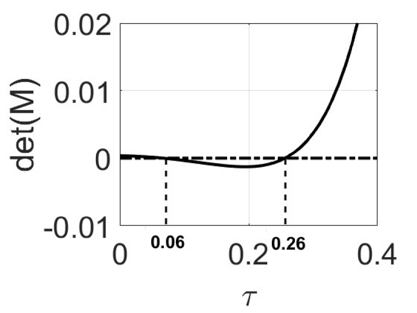
(a) Evolution of $\det(M)$

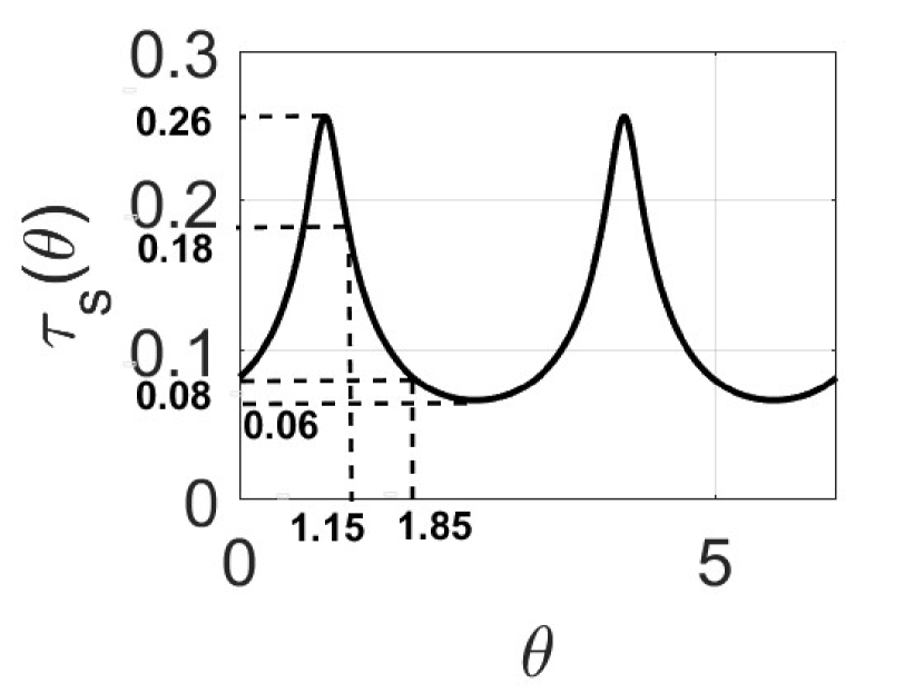
(b) Inter-event time function

(c) Evolution of $\det(L)$

(d) $\phi(\theta)-\theta$ map

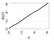
(e) Lift of the “angle” map

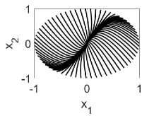
(f) Phase portrait

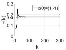
(g) Inter-event time evolution

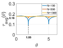
(h) Average inter-event time

Figure 1: Simulation results of Case 1 when $A_{c}$ has real eigenvalues at $\{-0.5528,-1.4472\}$.

Case 2:

In this case, we use the same $A$ matrix as in Case 1 but choose the input matrix $B=[0\quad 1]^{T}$ and the control gain $K=[0\quad-5]$ so that $A_{c}$ has complex conjugate eigenvalues at $\{-1+i,-1-i\}$. Figure 2 shows the simulation results for Case 2. For this case also the inter-event time function is continuous and periodic with period $\pi$. From Figure 2(a) and Figure 2(b) we can verify that $\det(M(\tau))=0$ has exactly two solutions and these two points are $\tau_{\min}$ and $\tau_{\max}$ respectively. Figure 2(c) shows that $\det(L(\tau))$ is always positive. Therefore the $\phi$ map in Figure 2(d) has no fixed point. As $\phi^{k}(.)$ map, for all $k\in\{1,2,3,4\}$, has no fixed point, we can say that the inter-event times does not converge to a steady state value for any initial condition. Figure 2(e) presents a lift of the “angle” map $\phi(.)$. As the lift $\Phi(.)$ is increasing monotonically, the “angle” map $\phi(.)$ is an orientation preserving homeomorphism. Figure 2(f) represents the phase portrait of the closed loop system. Figure 2(g) shows the evolution of inter-event times, for two arbitrary initial conditions, is oscillating in nature. Figure 2(h) presents the average inter-event time, for the total number of sampling instants equal to 1000, as a function of the angle of the initial state of the system. For this case, the average inter-event time is a constant for all inital states of the system. This may be due to several reasons. Either there does not exist a periodic orbit for the “angle” map or the “angle” map has a unique periodic orbit with period greater than one or the average inter-event time correspoding to all periodic orbits of the “angle” map is the same. It is not easy to distinguish between these cases from the simulation results.

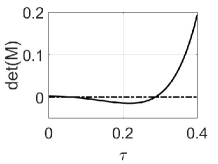
(a) Evolution of $\det(M)$

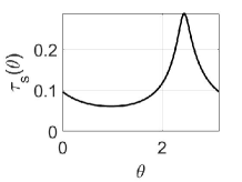
(b) Inter-event time function

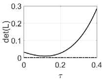
(c) Evolution of $\det(L)$

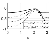
(d) $\phi^{k}(\theta)-\theta$ map

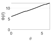
(e) Lift of the “angle” map

(f) Phase portrait of the closed loop system

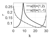
(g) Evolution of inter-event times

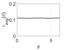
(h) Average inter-event time

Figure 2: Simulation results of Case 2 when $A_{c}$ has complex conjugate eigenvalues at $\{-1+i,-1-i\}$.

Case 3:

Consider another system,

$$\dot{x}=\begin{bmatrix}[r]0&1\\ -2&3\end{bmatrix}x+\begin{bmatrix}1&0\\ 0&1\end{bmatrix}u=:Ax+Bu.$$

The system matrix $A$ has real eigenvalues at $\{1,2\}$. The control gain $K=\begin{bmatrix}[r]-1&-0.8\\ 1.8&-4\end{bmatrix}$ so that $A_{c}$ has complex conjugate eigenvalues at $\{-1+0.2i,-1-0.2i\}$. Figure 3 shows the simulation results of this system for the event triggering rule (3b) with $\sigma=0.2251$. Figure 3(a) shows that the “angle” map $\phi(.)$ has two fixed points, where the larger one is a stable fixed point. Note that according to Proposition 16, there exists a fixed point for the “angle” map only if $\left\lVert R\right\rVert>1$. In this case, we can verify that $\left\lVert R\right\rVert=1.3136$. In Figure 3(b) the inter-event time is converging to a steady state value for two different initial conditions. Under the assumption of sufficiently small relative threshold parameters,  [20] says that if the eigenvalues of the closed loop system matrix $A_{c}$ are complex conjugates then the inter-event times oscillate in a near periodic manner. But, in this example we show that even if $A_{c}$ has only complex conjugate eigenvalues, the inter-event times may still converge to a steady state value. Note however, that we cannot claim that this is a counter-example to the results of [20] as the bound on the relative thresholding parameter for which their results hold is not explicitly stated.

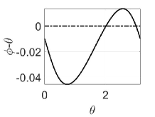
(a) $\phi(\theta)-\theta$ map

(b) Evolution of inter-event times

Figure 3: Simulation results of Case 3 when $A_{c}$ has complex conjugate eigenvalues at $[-1+0.2i,-1-0.2i]$.

Case 4:

Now consider the system,

$$\dot{x}=\begin{bmatrix}1&4\\ 0&1\end{bmatrix}x+\begin{bmatrix}0\\ 1\end{bmatrix}u=:Ax+Bu.$$

$A$ has real and equal eigenvalues at $\{1,1\}$. We let the control gain $K=[-2\quad-4]$, so that $A_{c}$ has eigenvalues at $\{-1+2i,-1-2i\}$. Figure 4 shows the simulation results of this system for the triggering rule (3a). Figure 4(a) shows that the inter-event time function $\tau_{s}(\theta)$ is discontinuous around $\theta=$ 2.3 radians. In Figure 4(b), we can see that around $\theta=2.3$ radians, there is a jump in the smallest $\tau$ value at which $f_{s}(\theta,\tau)=0$. This causes a point of discontinuity in the inter-event time function.

(a) Inter-event time function

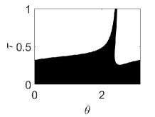
(b) 0-sub-level set of $f_{s}$

Figure 4: Simulation results of Case 4 with discontinuous inter-event time function.

7 Conclusion

In this paper, we analyzed the asymptotic behavior of inter-event times in planar linear systems under a general class of scale-invariant event-triggering rules. We first analyzed the properties, such as periodicity and continuity, of the inter-event time as a function of the “angle” of the state at an event triggering instant. We then analyzed the map that determines the evolution of the “angle” of the state from one event to the next. We provided a sufficient condition for the convergence or non-convergence of inter-event times to a steady state value under a scale-invariant event-triggering rule by analyzing the fixed points of the “angle” map. We also analyzed the stability and region of convergence of a fixed point of the “angle” map. We, then, analyzed the ergodicity of the “angle” map and with the help of ergodic theory, we provided a sufficient condition for the asymptotic average inter-event time to be a constant for all initial states of the system. Then, we considered a special case where the “angle” map is an orientation-preserving homeomorphism. Using rotation theory, we explained the asymptotic behavior of the inter-event times, including on whether the inter-event times converge to a periodic sequence. We also analyzed the asymptotic average inter-event time as a function of the angle of the initial state of the system. Finally, we illustrated the proposed results through numerical examples. Future work includes extensions of the analysis to discontinuous “angle” maps, extensions to systems of higher dimensions and possibly to nonlinear systems. Other potential research directions include development of algorithms that can estimate the asymptotic average inter-event times for different regions of the state space.

References

- [1] P. Tabuada, Event-triggered real-time scheduling of stabilizing control tasks, IEEE Transactions on Automatic Control 52 (9) (2007) 1680–1685.
- [2] W. Heemels, K. Johansson, P. Tabuada, An introduction to event-triggered and self-triggered control, in: 2012 IEEE 51st IEEE Conference on Decision and Control (CDC), 2012, pp. 3270–3285.
- [3] M. Lemmon, Event-triggered feedback in control, estimation, and optimization, in: Networked control systems, Springer, 2010, pp. 293–358.
- [4] D. Tolić, S. Hirche, Networked control systems with intermittent feedback, CRC Press, 2017.
- [5] F. D. Brunner, W. P. M. H. Heemels, F. Allgower, Robust event-triggered MPC with guaranteed asymptotic bound and average sampling rate, IEEE Transactions on Automatic Control 62 (11) (2017) 5694–5709.
- [6] P. Tallapragada, M. Franceschetti, J. Cortés, Event-triggered second-moment stabilization of linear systems under packet drops, IEEE Transactions on Automatic Control 63 (8) (2018) 2374–2388.
- [7] S. Bose, P. Tallapragada, Event-triggered second moment stabilisation under action-dependent Markov packet drops, IET Control Theory and Applications 15 (7) (2021) 949–964.
- [8] K. Astrom, B. Bernhardsson, Comparison of Riemann and Lebesgue sampling for first order stochastic systems, in: Proceedings of the 41st IEEE Conference on Decision and Control, Vol. 2, 2002, pp. 2011–2016.
- [9] B. Demirel, A. S. Leong, D. E. Quevedo, Performance analysis of event-triggered control systems with a probabilistic triggering mechanism: The scalar case, 20th IFAC World Congress 50 (1) (2017) 10084–10089.
- [10] P. Tallapragada, J. Cortés, Event-triggered stabilization of linear systems under bounded bit rates, IEEE Transactions on Automatic Control 61 (6) (2016) 1575–1589.
- [11] Q. Ling, Bit rate conditions to stabilize a continuous-time scalar linear system based on event triggering, IEEE Transactions on Automatic Control 62 (8) (2017) 4093–4100.
- [12] J. Pearson, J. P. Hespanha, D. Liberzon, Control with minimal cost-per-symbol encoding and quasi-optimality of event-based encoders, IEEE Transactions on Automatic Control 62 (5) (2017) 2286–2301.
- [13] M. J. Khojasteh, P. Tallapragada, J. Cortés, M. Franceschetti, The value of timing information in event-triggered control, IEEE Transactions on Automatic Control 65 (3) (2020) 925–940.
- [14] B. Asadi Khashooei, D. J. Antunes, W. P. M. H. Heemels, A consistent threshold-based policy for event-triggered control, IEEE Control Systems Letters 2 (3) (2018) 447–452.
- [15] F. D. Brunner, D. Antunes, F. Allgower, Stochastic thresholds in event-triggered control: A consistent policy for quadratic control, Automatica 89 (2018) 376 – 381.
- [16] P. Tallapragada, M. Franceschetti, J. Cortés, Event-triggered control under time-varying rate and channel blackouts, IFAC Journal of Systems and Control 9 (2019) 100064.
- [17] A. Anta, P. Tabuada, To sample or not to sample: Self-triggered control for nonlinear systems, IEEE Transactions on Automatic Control 55 (9) (2010) 2030–2042.
- [18] W. P. M. H. Heemels, M. C. F. Donkers, A. R. Teel, Periodic event-triggered control for linear systems, IEEE Transactions on Automatic Control 58 (4) (2013) 847–861.
- [19] M. Velasco, P. Martí, E. Bini, Equilibrium sampling interval sequences for event-driven controllers, in: European Control Conference (ECC), 2009, pp. 3773–3778.
- [20] R. Postoyan, R. G. Sanfelice, W. Heemels, Explaining the “mystery” of periodicity in inter-transmission times in two-dimensional event-triggered controlled system, IEEE Transactions on Automatic Control (2022).
- [21] A. Sharifi Kolarijani, M. Mazo, Formal traffic characterization of lti event-triggered control systems, IEEE Transactions on Control of Network Systems 5 (1) (2018) 274–283.
- [22] G. Delimpaltadakis, M. Mazo, Traffic abstractions of nonlinear homogeneous event-triggered control systems, in: 59th IEEE Conference on Decision and Control (CDC), 2020, pp. 4991–4998.
- [23] G. Delimpaltadakis, L. Laurenti, M. Mazo, Abstracting the sampling behaviour of stochastic linear periodic event-triggered control systems, in: 2021 60th IEEE Conference on Decision and Control (CDC), 2021, pp. 1287–1294.
- [24] G. de A. Gleizer, M. Mazo, Computing the sampling performance of event-triggered control, in: Proceedings of the 24th International Conference on Hybrid Systems: Computation and Control, 2021.
- [25] G. de Albuquerque Gleizer, M. Mazo, Computing the average inter-sample time of event-triggered control using quantitative automata, Nonlinear Analysis: Hybrid Systems 47 (2023) 101290.
- [26] G. d. A. Gleizer, M. Mazo, Chaos and order in event-triggered control, IEEE Transactions on Automatic Control (2023) 1–16.
- [27] A. Rajan, P. Tallapragada, Analysis of inter-event times for planar linear systems under a general class of event triggering rules, in: 59th IEEE Conference on Decision and Control (CDC), 2020, pp. 5206–5211.
- [28] A. Rajan, P. Tallapragada, Analysis of inter-event times in linear systems under region-based self-triggered control, arXiv preprint arXiv:2212.14273 (2022).
- [29] J. Souček, V. Souček, Morse-sard theorem for real-analytic functions, Commentationes Mathematicae Universitatis Carolinae 013 (1) (1972) 45–51.
- [30] N. Kryloff, N. Bogoliouboff, The general theory of measurement in its application to the study of dynamical systems of nonlinear mechanics, Annals of Mathematics 38 (1937) 65.
- [31] A. Katok, B. Hasselblatt, Introduction to the Modern Theory of Dynamical Systems, Encyclopedia of Mathematics and its Applications, Cambridge University Press, 1995.
- [32] P. Walters, An Introduction to Ergodic Theory, Graduate texts in mathematics, Springer-Verlag, 1982.
- [33] C. Arteaga, Unique ergodicity of continuous self-maps of the circle, Journal of Mathematical Analysis and Applications 163 (1992) 536–540.
- [34] M. Van Veldhuizen, On the numerical approximation of the rotation number, Journal of Computational and Applied Mathematics 21 (2) (1988) 203–212.
- [35] R. Pavani, A numerical approximation of the rotation number, Applied Mathematics and Computation 73 (1995) 191–201.
- [36] A. Belova, Rigorous enclosures of rotation numbers by interval methods, Journal of Computational Dynamics 3 (1) (2016) 81–91.