Exponential size scaling of the Liouvillian gap in boundary-dissipated systems with Anderson localization

Abstract

We carry out a systematical study of the size scaling of Liouvillian gap in boundary-dissipated one-dimensional quasiperiodic and disorder systems. By treating the boundary-dissipation operators as a perturbation, we derive an analytical expression of the Liouvillian gap, which indicates clearly the Liouvillian gap being proportional to the minimum of boundary densities of eigenstates of the underlying Hamiltonian, and thus give a theoretical explanation why the Liouvillian gap has different size scaling relation in the extended and localized phase. While the Liouvillian gap displays a power-law size scaling $\Delta_{g}\propto L^{-3}$ in the extended phase, our analytical result unveils that the Liouvillian gap fulfills an exponential scaling relation $\Delta_{g}\propto e^{-\kappa L}$ in the localized phase, where $\kappa$ takes the largest Lyapunov exponent of localized eigenstates of the underlying Hamiltonian. By scrutinizing the extended Aubry-André-Harper model, we numerically confirm that the Liouvillian gap fulfills the exponential scaling relation and the fitting exponent $\kappa$ coincides pretty well with the analytical result of Lyapunov exponent. The exponential scaling relation is further verified numerically in other one-dimensional quasiperiodic and random disorder models. We also study the relaxation dynamics and show the inverse of Liouvillian gap giving a reasonable timescale of asymptotic convergence to the steady state.

I Introduction

In the past years, advances in manipulating dissipation and quantum coherence in laboratory have led to a renewed interest in the study of open quantum systems with intriguing dissipative dynamics (Weimer2021RMP, ; Diehl2008, ; Cirac2009, ; CaiZ, ; Prosen2012, ; Zhong2019PRL, ; LiuCHPRR, ; Poletti, ; Prosen2008NJP, ; Ueda, ). Understanding dynamical processes evolving to steady states in open quantum systems driven by boundary dissipations is a central problem of out-of-equilibrium statistical physics attracted intensive theoretical studies Prosen2008PRL ; Prosen2014PRL ; Znidaric2015PRE ; GuoC2018 ; Yoo ; Popkov ; Lacerda ; Shibata2020PTEP ; Popkov2013 ; Vicari ; Znidaric2021 ; Znidaric2017 ; Schulz ; Carollo ; Briegel2013PRE ; Znidaric2010JSM ; Popkov2016PRA ; ZhouZW ; Monthus ; Schaller2021arXiv Within the Markovian approximation, the density matrix of the system evolves according to the Lindblad master equation with the Liouvillian gap $\Delta_{g}$ defined as the smallest modulus of the real part of nonzero eigenvalues of the Liouvillian superoperator. Usually, the inverse of the Liouvillian gap gives an estimation on the timescale of the relaxation time CaiZ ; Prosen2008NJP ; Znidaric2015PRE . Although discrepancy between the inverse of Liouvillian gap and the relaxation time is found in some recent works Ueda ; Znidaric2015PRE ; Mori ; Mori2021PRR ; Bensa2022PRR , the Liouvillian gap is still an important quantity characterizing the asymptotic convergence to the steady state Mori ; Schaller2021arXiv ; DengDL . Numerical results have demonstrated that the Liouvillian gap scales with the system length $L$ in terms of $L^{-z}$ for various boundary-dissipated systems Znidaric2015PRE ; Shibata2020PTEP ; Mori ; Prosen2008PRL , where $z\in[1,2)$ for chaotic systems and $z=3$ for integrable systems.

While most previous studies focus on the homogeneous systems, less is known for the relaxation dynamics in disorder systems with boundary dissipation. As localization has been recognized as important physical implication of interference of waves in dissipative media, recently there is growing interesting in the disorder effect on non-Hermitian physics Hatano ; ZengQB ; JiangH ; Longhi ; LiuYX ; Hughes ; Ryu ; ZhangDW ; XuY and open quantum systems Denisov ; Luitz ; Can , as well as the dynamical effect of Anderson localization induced by the Markovian noise Lorenzo ; Lezama . In Ref.Prosen2008NJP , Prosen has provided numerical evidence that the Liouvillian gap of the boundary-dissipated disordered XY chain is exponentially small, i.e., $\Delta_{g}\propto e^{-L/\ell}$ with $\ell$ being the localization length of normal master mode. Although the numerical result in Ref.Prosen2008NJP suggests that the Liouvillian gap should fulfill an exponential scaling relation with the system length, a theoretical analysis and systematic study of the Liouvillian gap for disorder systems with boundary dissipations are still lacking. For a 1D disordered system, the localization length of a localized eigenstate is usually energy dependent, and thus the localization length of normal master mode is expected to be mode dependent, so the meaning of $\ell$ is somewhat ambiguous. Natural questions arising here are how to understand the role of normal master modes in the formation of the Liouvillian gap and the connection of Liouvillian gap to the localization lengths of eigenstates of the underlying disordered chain?

To understand how the Liouvillian gap is affected by the disorder, we first carry out a perturbative calculation by treating the boundary-dissipation operators as a perturbation and give an analytical derivation of the Liouvillian gap on the basis of perturbation theory. Our analytical result indicates that the size of Liouvillian gap is proportional to the minimum of boundary densities of eigenstates of the underlying Hamiltonian, and thus the Liouvillian gap displays an exponential size scaling when the underlying system possesses localized eigenstates. To get an intuitive understanding from concrete examples, we then study the scaling relation of Liouvillian gap numerically for various one-dimensional quasiperiodic and disorder systems with boundary dissipations described by the Lindblad master equation. The first example we consider is the extended Aubry-André-Harper (AAH) model with boundary dissipations. One of the reason for choosing the extended AAH model is that it exhibits rich phase diagram with extended (or delocalized), critical and localized phases depending on the quasiperiodical modulation parameters Hatsugai ; Takada ; HanJH ; WangYC , and the other reason is that the Lyapunov exponent (inverse of the localization length) of the localized eigenstate of the model has an analytical expression which is very helpful for checking our numerical fitting results. Our numerical results illustrate that Liouvillian gap $\Delta_{g}$ displays different features in the underlying distinct phase regions. While $\Delta_{g}\propto L^{-3}$ in the extended phase, the Liouvillian gap scales with $L$ in an exponential way $e^{-aL}$ in the localized phase, where $a$ is identified to be identical to the Lyapunov exponent $\kappa$ of the localized state. To confirm the validity of the exponential scaling relation, we further study a quasiperiodical model with mobility edge and the 1D Anderson lattice, in which the localization length of a localized eigenstate is energy dependent. Our numerical results show that the Liouvillian gap displays similar exponential scaling relation $e^{-aL}$ with $a$ determined by the Lyapunov exponent of states in the band edges.

The rest of paper is organized as follows. In Sec. II A, we introduce the formalism for the calculation of Liouvillian gap and present the analytical derivation of Liouvillian gap in the scheme of perturbation theory. In Sec.II B, we first study the scaling relation of Liouvillian gap in the boundary-dissipated extended AAH model, and then extend our study to the boundary-dissipated quasiperiodic model with mobility edge and the 1D Anderson model. In Sec.II C, we discuss the relaxation time by numerically studying the dynamical evolution of average occupation number. A summary is given in the last section.

II Formalism, models and results

II.1 Formalism and perturbative calculation of Liouvillian gap

We consider open systems with the dissipative dynamics of density matrix $\rho(t)$ governed by the Lindblad master equation Lindblad ; GKS :

$$\frac{d\rho}{dt}=\mathcal{L}\left[\rho\right]=-i\left[H,\rho\right]+\sum_{\mu}\left(2L_{\mu}\rho L_{\mu}^{\dagger}-\left\{L_{\mu}^{\dagger}L_{\mu},\rho\right\}\right),$$ (1)

where $H$ is the Hamiltonian governing the unitary part of dynamics of the system and $L_{\mu}$ are the Lindblad operators describing the dissipative process with the index $\mu$ denoting the dissipation channels. Particularly, we consider the boundary-dissipated systems with the Lindblad operators acting only on the first and the last site of the lattice and taking the form of

$$L_{1}=\sqrt{\gamma_{1}}c_{1},\,\,\,\,\,\,\,\,\,\,\,\,L_{L}=\sqrt{\gamma_{L}}c_{L},$$ (2)

where $c_{j}$ is the fermion annihilation operator acting on the site $j$ and $\gamma_{1}$ ($\gamma_{L}$) denotes the boundary dissipation strength. In this work, we shall consider 1D quasiperiodic and disorder fermion systems with quasiperiodic or random on-site potentials described by the Hamiltonian

$$H=\sum_{i=1}^{L-1}J_{i}(c_{i}^{\dagger}c_{i+1}+c_{i+1}^{\dagger}c_{i})+\sum_{i=1}^{L}V_{i}c_{i}^{\dagger}c_{i},$$ (3)

where $J_{i}$ represents the hopping amplitude between the $i$-th and $(i+1)$-th sites and $V_{i}$ denotes the chemical potential on the $i$-th site. Since the Hamiltonian is quadratic in fermionic operators, Eq. (1) with linear dissipations also takes a quadratic form. For a quadratic open fermionic model with $L$ sites, solving for the Liouvillian gap of the quantum Lindblad equation can be reduced to the diagonalization of a $4L\times 4L$ antisymmetric matrix (Prosen2008NJP, ) or $L\times L$ non-Hermitian matrix (Poletti, ; Zhong2019PRL, ).

In Ref.Zhong2019PRL , it is shown that the Liouvillian gap can be obtained by

$$\Delta_{g}=\min[2\text{Re}(-\beta_{n})],$$ (4)

where $\beta_{n}$ is the eigenvalue of damping matrix given by (Zhong2019PRL, )

$$X=ih^{T}-\left(M_{1}+M_{L}\right)^{T}$$ (5)

with $\left(h\right)_{jk}=J_{j}(\delta_{j,k+1}+\delta_{j+1,k})+V_{j}\delta_{jk}$, $\left(M_{1}\right)_{jk}=\delta_{j1}\delta_{k1}\gamma_{1}$ and $\left(M_{L}\right)_{jk}=\delta_{jL}\delta_{kL}\gamma_{L}$. By numerical diagonalization of the damping matrix $X$ for systems with different $L$, we can explore the size scaling relation of the Liouvillian gap for the quasiperiodic or disorder chain with boundary dissipations. Before studying the concrete models, we shall use perturbation theory to derive an analytical expression of the Liouvillian gap under the weak dissipation limit, which is very helpful for understanding the scaling relation of Liouvillian gap.

By using Jordan-Wigner transformation to replace fermion creation and annihilation operators with spin operators, $c_{i}^{\dagger}=P_{i}\sigma_{i}^{+}$, $c_{i}=P_{i}\sigma_{i}^{-}$, $P_{i}=\prod_{k=1}^{i-1}\sigma_{k}^{z}$, and introducing the Choi-Jamiolkwski isomorphism Choi ; Jamiolkowski ; Tyson ; Vidal which turns the matrix into a vector:

$$\rho=\sum_{mn}\rho_{mn}|m\rangle\langle n|\ \rightarrow\ |\rho\rangle=\sum_{mn}\rho_{mn}|m\rangle\otimes|n\rangle,$$

the Lindblad equation can then be rewritten into the vectorized form

$$\frac{d|\rho(t)\rangle}{dt}=\mathbb{L}|\rho(t)\rangle=(\mathbb{L}_{0}+\mathbb{L}_{1})|\rho(t)\rangle,$$ (6)

where explicit forms of $\mathbb{L}_{0}$ and $\mathbb{L}_{1}$ are given in the appendix A.

By virtue of the parity operator $Q=\prod_{k=1}^{L}\sigma_{k}^{z}\tau_{k}^{z}$, which satisfies $[Q,\mathbb{L}]=0$ and has eigenvalues of $\pm 1$, we can define the projection operators $\mathcal{Q}_{\pm}=(1\pm Q)/2$ such that $\mathbb{L}=\mathbb{L}_{+}\bigoplus\mathbb{L}_{-}=(\mathcal{Q}_{+}\mathbb{L}\mathcal{Q}_{+})\bigoplus(\mathcal{Q}_{-}\mathbb{L}\mathcal{Q}_{-})$. Since the parity operator only appears in $\mathbb{L}_{1}$, we have $\mathcal{Q}_{+}\mathbb{L}_{0}\mathcal{Q}_{+}=\mathcal{Q}_{-}\mathbb{L}_{0}\mathcal{Q}_{-}=\mathbb{L}_{0}$. It can be proved that in the specific model we studied, the Liouvillian gap is not affected by the choice of parity when only considering perturbation to first-order correction, so we only need to consider $\mathbb{L}_{+}=\mathbb{L}_{0+}+\mathbb{L}_{1+}$ with

$$\begin{array}[]{cl}\mathbb{L}_{0+}=&\mathbb{L}_{0}=-i\left(\widetilde{H}\otimes\mathbb{I}-\mathbb{I}\otimes\widetilde{H}^{T}\right),\\ \mathbb{L}_{1+}=&\mathcal{Q}_{+}\mathbb{L}_{1}\mathcal{Q}_{+}=\sum_{\mu}\left[2\widetilde{L_{\mu}}\otimes\widetilde{L_{\mu}}^{*}-(\widetilde{L_{\mu}}^{\dagger}\widetilde{L_{\mu}})\otimes\mathbb{I}\right.\\ &\left.-\mathbb{I}\otimes(\widetilde{L_{\mu}}^{\dagger}\widetilde{L_{\mu}})^{T}\right],\ \ \mu=1,L\end{array}$$ (7)

where $\widetilde{H},\ \widetilde{L_{1}},\ \widetilde{L_{L}}$ differ from $H,\ L_{1},\ L_{L}$ only by replacing fermion operators $c_{i},\ c_{i}^{\dagger}$ with spin operators $\sigma_{i}^{-},\ \sigma_{i}^{+}$ (see Appendix A for details).

Taking $\mathbb{L}_{1+}$ as a perturbation to $\mathbb{L}_{0+}$ and considering only the first-order perturbation, we assume that the eigenvalues $\eta_{r,s}^{(0)}$ without perturbation are $d(r,s)$-fold degenerate, and the corresponding eigenvectors are denoted as set $\{|\Psi_{r,s}\rangle\}$, where $|\Psi_{r,s}\rangle:=|\psi_{r}\rangle\otimes|\psi_{s}\rangle^{*}$ is the right eigenvector of $\mathbb{L}_{0+}$ with both $|\psi_{r}\rangle$ and $|\psi_{s}\rangle$ being the eigenvectors of $\widetilde{H}$. It can be known that the first-order perturbation to eigenvalues of Liouvillian superoperator $\mathbb{L}_{+}$, denoted by $\eta_{r,s}^{(1)}$, are the eigenvalues of matrix $W$ with matrix elements $W_{k,k^{\prime}}=\langle\Psi_{k}|\mathbb{L}_{1+}|\Psi_{k^{\prime}}\rangle:=\langle\Psi_{r,s}|\mathbb{L}_{1+}|\Psi_{r^{\prime},s^{\prime}}\rangle$, where $|\Psi_{k^{\prime}}\rangle\equiv|\Psi_{r^{\prime},s^{\prime}}\rangle$ and $|\Psi_{k}\rangle\equiv|\Psi_{r,s}\rangle$ have the same zero order eigenvalue $\eta_{r,s}^{(0)}$.

Considering $[\widetilde{H},N]=0$, where $N=\sum_{j=1}^{L}\sigma_{i}^{+}\sigma_{i}^{-}$, we can order the degenerate eigenstates $|\Psi_{r,s}\rangle$ with the same eigenvalue $\eta_{r,s}^{0}$ from the smallest to largest in order of $N_{r,s}\equiv\langle\psi_{r}|N|\psi_{r}\rangle+\langle\psi_{s}|N|\psi_{s}\rangle$. Simple analysis shows that the first term of $\mathbb{L}_{1+}$ has no effect on the eigenvalues of $W$ and thus does not contribute to $\eta_{r,s}^{(1)}$. Then we obtain the Liouvillian spectrum

$$\eta=i(E_{r}-E_{s})-\sum_{\mu}\gamma_{\mu}(n_{\mu}^{r}+n_{\mu}^{s})$$ (8)

under the first order approximation and the Liouvillian gap

$$\Delta_{g}=\underset{\eta}{\min}^{\prime}\{\Re(-\eta)\}=2\underset{r}{\min}^{\prime}\{\sum_{\mu}\gamma_{\mu}n_{\mu}^{r}\},$$ (9)

in which both $E_{r}$ and $E_{s}$ being the eigenvalues of the Hamiltonian and $n_{\mu}^{r}\equiv\langle\psi_{r}|\sigma_{\mu}^{+}\sigma_{\mu}^{-}|\psi_{r}\rangle$, $\underset{r}{\min}^{\prime}\{x_{r}\}\equiv\underset{r}{\min}\{x_{r}|x_{r}\neq 0\}$. In our model, $\mu=1,L$, it can be seen that the Liouvillian gap corresponds to the minimum of nonzero sum of $2(\gamma_{1}n_{1}^{r}+\gamma_{L}n_{L}^{r})$, where $n_{1}^{r}$ ($n_{L}^{r}$) represents the left (right) boundary density of the $r$-th eigenstate of the underlying Hamiltonian $H$. For the case $\gamma_{1}=\gamma_{L}=\gamma$, we have

$$\Delta_{g}=2\gamma\underset{r}{\min}^{\prime}(n_{1}^{r}+n_{L}^{r}),$$ (10)

which indicates that the Liouvillian gap is proportional to the minimum of boundary densities of eigenstates of the underlying Hamiltonian.

Now we apply Eq.(10) to give a theoretical interpretation for the different scaling relations of Liouvillian gap in localized and extended phases. For simplicity, we shall focus on the case of $\gamma_{1}=\gamma_{L}=\gamma$ in the following discussions and calculations. Eq.(10) does not rely on the details of underlying Hamiltonian, and the Liouvillian gap is only relevant to the boundary densities of eigenstates of $H$. For the non-interacting Hamiltonian described by Eq.(3), solving Liouvillian gap only needs to consider the single particle space of the Hamiltonian. When the system is in a localized phase, the modulus of a localized wavefunction can be approximately described by $|\psi_{r}(j)|\propto e^{-|j-r_{0}|/\xi_{r}}$, where $r_{0}$ is the index of the localization center and $\xi_{r}$ is the localization length. Then the corresponding density distribution is given by $n_{j}^{r}\propto e^{-2\kappa_{r}\left|j-r_{0}\right|}$, where $\kappa_{r}=1/\xi_{r}$ is the Lyapunov exponent of the localized eigenstate. For the quasiperiodic system described by the extended AAH model (see Eq.(14)), all eigenstates have the same localization length and Lyapunov exponent, and thus we can denote the state-independent Lyapunov exponent as $\kappa$ (given by Eq.(15) for the extended AAH model). The different localized eigenstate with the same localization length can be characterized by different localization center $r_{0}$, i.e., $n_{j}^{r}\propto e^{-2\kappa\left|j-r_{0}\right|}$. Then we can estimate the Liouvillian gap by using Eq.(10), which gives rise to

$$\Delta_{g}\propto 2\gamma\underset{r_{0}}{\min}^{\prime}\{e^{-2\kappa(r_{0}-1)}+e^{-2\kappa(L-r_{0})}\}\propto\gamma e^{-\kappa L}.$$ (11)

In general, the Lyapunov exponent of a localized eigenstate of quasiperiodic and disordered systems is state-dependent, e.g., the Lyapunov exponent of a localized eigenatate of the quasiperiodic model (18) is given by Eq.(19), which is energy dependent. The Lyapunov exponent $\kappa(E)$ takes its maximum in the top of energy band, and thus applying Eq.(10) we can estimate

$$\Delta_{g}\propto\gamma e^{-\kappa(E_{\text{top}})L},$$ (12)

where $E_{\text{top}}$ represents the eigenvalue of the localized eigenstate on the top of energy band.

Now we apply Eq.(10) to give a theoretical interpretation for the scaling relation of Liouvillian gap $\Delta_{g}\propto L^{-3}$ in the extended phase. For simplicity, we consider an extreme case of Hamiltonian (3) with $J_{i}=1$ and $V_{i}=0$, then we have $n_{\mu}^{r}=\frac{2}{L+1}\sin^{2}\left(k_{r}\mu\right)$, where $k_{r}=\frac{r\pi}{L+1}$. By using Eq.(10), it follows

$$\begin{array}[]{cl}\Delta_{g}&=2\gamma(n_{1}^{1}+n_{L}^{1})=\frac{8\gamma}{L+1}\sin^{2}\left(\frac{\pi}{L+1}\right)\\ &\approx 8\gamma\pi^{2}L^{-3}\propto\gamma L^{-3},\end{array}$$ (13)

which is consistent with results in references Prosen2008NJP ; Znidaric2015PRE .

II.2 Liouvillian gap in boundary-dissipated quasiperiodic and disorder systems

Our perturbative derivation of Liouvillian gap does not depend on the details of Hamiltonian. Eq.(10) suggests that the Liouvillian gap is closely related to the minimum of boundary densities of eigenstates of the underlying Hamiltonian. As long as $H$ supports localized eigenstates, similar argument holds true by following the procedure of deriving Eq.(12), and thus we expect the exponential scaling relation of Liouvillian gap is quite universal. To get an intuitive understanding, next we numerically study the scaling relation of Liouvillian gap in various boundary-dissipated quasiperiodic and disorder systems with equal boundary dissipation strengthes $\gamma_{1}=\gamma_{L}=\gamma$.

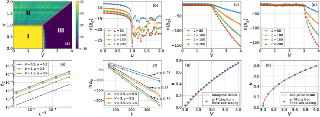
Figure 1: (a) $\ln\Delta_{g}$ with respect to $V$ and $u$ for $L=200$ and $\gamma=1$. The dashed lines denote the phase boundaries of the underlying phase diagram of the extended AAH model. (b) $\ln\Delta_{g}$ versus $u$ for various size of lattices with $V=0.5$. $\ln\Delta_{g}$ versus $V$ for various size of lattices with (c) $u=0.5$ and (d) $u=1.5$. Finite size scaling of Liouvillian gap in (e) the extended phase and (f) the localized phase, where the black dashed lines guide the value of $\Delta_{g}=L^{-3}$ and $\Delta_{g}=e^{-\kappa L}$, respectively. Here $L=55,89,144,233,377$ are chosen as the Fibonacci numbers. Comparing the numerical fitting data $a$ obtained from the finite size scaling with the analytical result of Lyapunov exponent for (g) $u=0.5$ and (h) $u=1.5$. The data of (g) and (h) are the same as (c) and (d) in localized phase, respectively.

To be concrete, we first consider the quasiperiodic system with $H$ described by the extended AAH model Hatsugai ; Takada ; HanJH :

$$H= J\sum_{j=1}^{L-1}\left\{1+u\cos\left[2\pi(j+\frac{1}{2})\alpha\right]\right\}\left(c_{j}^{\dagger}c_{j+1}+\text{H.c.}\right)$$

$$+V\sum_{j=1}^{L}\cos\left(2\pi j\alpha\right)c_{j}^{\dagger}c_{j},$$ (14)

where $\alpha=(\sqrt{5}-1)/2$, the hopping strength $J$ defines the energy scale and is set to 1, $c_{j}^{\dagger}(c_{j})$ is the fermion creation (annihilation) operator, $u$ represents the modulation amplitude for the off-diagonal hopping, and $V$ is the strength of the on-site quasiperiodic potential. In the absence of boundary dissipations, the phase diagram of AAH model is shown in the Fig. 1(a) with the regions I, II and III corresponding to extended, critical, and localized phases, respectively Hatsugai ; Takada ; HanJH . The phase boundaries can be obtained with finite-size scaling analyses for the wavefunction properties and level statistics Hatsugai ; Takada ; HanJH . For the extended AAH model (14), we note that the Lyapunov exponent can be analytically expressed as Jitomirskaya ; HanJH

$$\kappa=\begin{cases}\max\left\{\ln\left|\frac{\left|V\right|+\sqrt{V^{2}-4u^{2}}}{2u}\right|,0\right\},&\left|u\right|\geqslant 1\\ \max\left\{\ln\left|\frac{\left|V\right|+\sqrt{V^{2}-4u^{2}}}{2\left(1+\sqrt{1-u^{2}}\right)}\right|,0\right\}.&\left|u\right|<1\end{cases}$$ (15)

By using the above analytical result, the phase boundaries between localized phase and extended (critical) phase can be analytically determined.

Without loss of generality, we fix $\gamma=1$ and calculate the Liouvillian gap for various parameters $u$ and $V$. The value of $\ln(\Delta_{g})$ is displayed in the underlying phase diagram in Fig.1(a), which indicates the Liouvillian gap exhibiting different features in different phase regions. As shown in Fig. 1(b)-(d), $\ln(\Delta_{g})$ also displays an abrupt change in the phase boundaries of the underlying phase diagram. By analyzing the size scaling of $\Delta_{g}$ as shown in Fig.1(e), we demonstrate that the Liouvillian gap in the extended region fulfills

$$\Delta_{g}(L)\propto L^{-3},$$ (16)

which is consistent with Eq.(13). In the critical region, the Liouvillian gap approximately fulfills the algebraic form

$$\Delta_{g}(L)\propto L^{-\eta},$$

where $\eta>3$ is a non-universal exponent sensitive to parameters of $u$ and $V$. The sensitivity to parameter $u$ can be also witnessed by the oscillation behavior in Fig.1(b). For the localized phase, the finite size scaling of $\Delta_{g}$ in Fig.1(f) shows the Liouvillian gap taking the exponential form:

$$\Delta_{g}(L)\propto e^{-aL},$$ (17)

where $a$ is a parameter-dependent constant. Our numerical results unveil that $a$ is identical to the Lyapunov exponent of the localized phase with $\kappa$ given by Eq.(15), which is obviously independent of eigenvalues of localized states. In Fig. 1(g) and (h), we plot the Lyapunov exponent versus $V$ according to Eq. (15) by taking $u=0.5$ and $1.5$, respectively, in comparison with the numerical fitting data $a$ obtained from the finite size scaling, which indicates clearly $a\approx\kappa$ in the whole underlying localized region.

To scrutinize the scaling relation for more complex quasiperiodic systems, next we consider a quasiperiodic system with a mobility edge described by the following Hamiltonian Ganeshan :

$$H=J\sum_{j=1}^{L-1}\left(c_{j}^{\dagger}c_{j+1}+\text{H.c.}\right)+2\lambda\sum_{j=1}^{L}\frac{\cos\left(2\pi\alpha j\right)}{1-b\cos\left(2\pi\alpha j\right)}c_{j}^{\dagger}c_{j},$$ (18)

where $\alpha=(\sqrt{5}-1)/2$ and $b\in(-1,1)$, the hopping strength $J$ defines the energy scale and is set to 1. While Eq. (18) reduces to the AAH model for $b=0$, the model with $b\neq 0$ exhibits an exact mobility edge following the expression $E=2\,\text{sgn}(\lambda)(1-|\lambda|)/b$. The Lyapunov exponent for the localized state can be obtained from $\kappa(E)=\max\left\{\kappa_{c}(E),0\right\}$ with the analytical expression of $\kappa_{c}(E)$ given by LiuYX2 ; XiaX

$$\kappa_{c}(E)=\ln\left|\frac{\left|bE+2\lambda\right|+\sqrt{\left(bE+2\lambda\right)^{2}-4b^{2}}}{2\left(1+\sqrt{1-b^{2}}\right)}\right|,$$ (19)

where $E$ denotes the eigenvalue of Eq. (18). In Fig. 2(a), we show the energy spectrum with respect to $\lambda$ of Eq. (18) with $b=0.2$ and the value of $\kappa(E)$ is denoted by the color. The mobility edge can be determined by $\kappa_{c}(E)=0$, as illustrated by the blue solid line in Fig.2(a), which separates the extended states from the localized states above it. It can be seen that the non-zero value of the Lyapunov exponent would appear in spectrum as $\lambda$ increases across the mobility edge.

By fixing the boundary dissipation strength $\gamma=1$, we display the Liouvillian gap with respect to $\lambda$ in Fig. 2(b) for different system sizes. When $\lambda$ exceeds a critical value, corresponding to the emergence of mobility edge, the size scaling relation of Liouvillian gap has an obvious change. The finite size analysis demonstrates that the Liouvillian gap fulfills an exponential form $\Delta_{g}\propto e^{-aL}$. The exponent $a$ with respect to $\lambda$ extracted from the exponential fitting of the data is shown in the Fig. 2(c), which is found to agree well with $\kappa(E_{\text{top}})$, where $E_{\text{top}}$ denotes the eigenvalue in the top of the energy band with the corresponding Lyapunov exponent taking the largest value. It turns out that the size scaling of Liouvillian gap for this quasiperiodic model can be well described by $\Delta_{g}\propto e^{-\kappa(E_{\text{top}})L}$, consistent with Eq.(12) as predicted by our theoretical analysis.

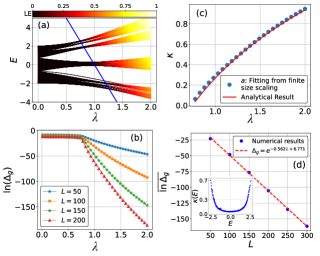
Figure 2: (a) Energy spectrum of Eq.(18) with respect to $\lambda$ for $L=200$ with the color representing the value of Lyapunov exponent of the eigenstate with the corresponding eigenvalue. The blue solid line represents the exact mobility edge. (b) $\ln\Delta_{g}$ versus $\lambda$ for various size of lattices with $b=0.2$; (c) Comparing the numerical fitting data $a$ obtained from the finite size scaling with the analytical result of Lyapunov exponent. (d) Finite size scaling of $\ln\Delta_{g}$ for 1D Anderson model by averaging 100 samples. The insert in (d) shows the Lyapunov exponent of 1D Anderson model for $L=200$ by averaging 1000 samples.

Finally, we study the boundary-dissipated 1D Anderson model Schulz with $H$ described by

$$H=J\sum_{j=1}^{L-1}\left(c_{j}^{\dagger}c_{j+1}+\text{H.c.}\right)+\sum_{j=1}^{L}V_{j}c_{j}^{\dagger}c_{j},$$ (20)

where the on-site random potential $V_{j}$ uniformly distributes among $[-V,V]$, the hopping strength $J$ defines the energy scale and is set to 1. For the 1D Anderson model, the state is always localized for arbitrarily weak disorder strength $V$. By taking $\gamma=1$ and $V=1$, we calculate the Liouvillian gap numerically and find it also fulfills exponential size scaling relation $\Delta_{g}\propto e^{-aL}$ with $a\approx 0.562$, as shown in Fig. 2(d). As no analytical expression for the Lyapunov exponent of the Anderson model is available, we can numerically calculate the Lyapunov exponent by using $\kappa\left(E\right)=\ln\left(\max\left(\theta_{i}^{+},\theta_{i}^{-}\right)\right)$, where $\theta_{i}^{\pm}$ represents eigenvalues of the matrix $\mathbf{\Theta}=\left(T_{L}^{{\dagger}}T_{L}\right)^{1/(2L)}$ and

$$T_{L}\left(E,\theta\right)=\prod_{j=1}^{L}T^{j}=\prod_{j=1}^{L}\left(\begin{array}[]{cc}E-V_{j}&-1\\ 1&0\end{array}\right)$$

is the transfer matrix LiuYX . The numerical value of Lyapunov exponent versus $E$ for $V=1$ is displayed in the inset of Fig. 2(d). The numerical result indicates that the Lyapunov exponent for the Anderson model takes its maximum on the band edges. Since the center of localized wave function randomly distributes on the lattice site, we take an average over 10 states close to the band edges, which gives a mean value of Lyapunov exponent $\bar{\kappa}\approx 0.589\pm 0.066$. It can be seen that $\bar{\kappa}$ matches well with $a\approx 0.562$, i.e., the decaying exponent can be described by the mean value of Lyapunov exponent close to band edges of the 1D Anderson model.

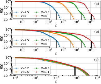
Figure 3: The average occupation number $\overline{n}(t)$ in the localized region of boundary-dissipated generalized AAH model for the initial state chosen as (a) the state localized at the center site 16; (b) the fully occupied state. (c) $\overline{n}(t)$ in the extended region with the fully occupied initial state. The black lines guide values of the inverse of Liouvillian gaps corresponding to different $V$. Here we have taken $L=30$, $u=0.2$ and $\gamma=1$.

II.3 Relaxation dynamics

To see clearly how the relaxation timescale related to the Liouvillian gap, we study the dynamical evolution of the average occupation number for the extended AAH model with boundary dissipation. The average occupation number is defined as $\overline{n}(t)=\sum_{j=1}^{L}\langle n_{j}(t)\rangle/[\sum_{j=1}^{L}\langle n_{j}(t=0)\rangle]$, where $\langle n_{j}(t)\rangle=\text{Tr}[\rho(t)c_{j}^{\dagger}c_{j}]$. We demonstrate $\overline{n}(t)$ versus $t$ for the system of $L=30$, $u=0.2$, $\gamma=1$ and various $V$ with the initial state chosen as the state localized at the center site $16$ in Fig. 3(a) and a fully occupied state in Fig. 3(b), respectively. For the open system with pure loss dissipation, the nonequilibrium steady state is the empty state with $\overline{n}(t\rightarrow\infty)=0$. Since the late-stage dynamics of the system near a steady state is governed by eigenmodes of Liouvillian whose eigenvalues are close to zero, the relaxation times can be estimated by the inverse of Liouvillian gaps, which are labeled by the black lines in the Fig. 3 for guidance. It can be observed that the inverse of Liouvillian gap gives a reasonable timescale for estimating the time of asymptotic convergence to the steady state. With the increase in $V$, the relaxation time in the localized phase increases quickly in terms of $\tau\propto e^{\kappa L}$, which can be approximately represented as $\tau\propto|V|^{L}$ and is much longer than the relaxation time in the extended state as shown in Fig. 3(c).

Next we show the evolution of $\overline{n}(t)$ for the boundary-dissipated 1D Anderson model with $L=30$, $\gamma=1$ and various $V$. The initial state in Fig. 4(a) is chosen as the state localized at the center site 16, and in Fig. 4(b) is the fully occupied state. For guidance, we also mark the values of the inverse of Liouvillian gaps by the black dashed lines in the figures. The dynamical evolution displays similar behaviors as in the localized phase of the quasiperiodic system. In can be found that the relaxation time increases quickly as the strength of random potential $V$ increases. Since the states in the 1D Anderson model are always localized, the relaxation time increases exponentially with the increase of system size for any nonzero disorder strength $V$.

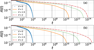
Figure 4: The average occupation number $\overline{n}(t)$ of 1D Anderson model for the initial state chosen as (a) the state localized at the center site 16; (b) the fully occupied state. The black lines guide values of the inverse of Liouvillian gaps corresponding to different $V$. Here we take $L=30$ and averaged 1000 samples for $V>0$.

III Summary and outlook

In summary, we study the size scaling relation of Liouvillian gap of boundary-dissipated 1D quasiperiodic and disorder systems both analytically and numerically. In the framework of perturbation theory, we give an analytical derivation of the Liouvillian gap by taking the boundary-dissipation terms as a perturbation. Our analytical result unveils that the Liouvillian gap is proportional to the minimum of boundary densities of eigenstates of the underlying Hamiltonian, and thus gives a theoretical explanation why the Liouvillian gap fulfills different size scaling relations when the underlying system is in the extended, critical and localized phase. When the underlying Hamiltonian has localized eigenstates, the Liouvillian gap displays an exponential size scaling with the decay exponent determined by the largest Lyapunov exponent of the localized eigenstates. The exponential size scaling relation was numerically verified in various quasiperiodic and disorder systems. By studying the dynamical evolution of average occupation number, we show that the inverse of Liouvillian gap gives a reasonable timescale for estimating the relaxation time.

The quasiperiodic optical lattices have provided an ideal platform for studying the localization transition in one dimension Bloch2018 ; Roati , and schemes for engineering quasiperiodic optical lattices in open quantum systems are proposed through purely dissipative processes YiW ; LiuYG . Manipulation of laser-induced dissipations LuoL at the boundaries allows us to study the relaxation dynamics of the quasiperiodic lattices. As the localization length in quasiperiodic optical lattice can be tuned by engineering the strength of incommensurate potential, we expect that the relation between the relaxation time and the localization length of boundary-dissipated quasiperiodic lattice could be unveiled in the experiment. By considering the interaction effect, it is interesting to study the stability of the many-body localized phase subjected to boundary dissipation both theoretically Sels and experimentally.

Appendix A First-order degenerate perturbation of Liouvillian gap

In this appendix, we give details of the perturbative calculation of Liouvillian gap.

A.1 Matrix representation of Liouvillian superoperators

We consider a dissipative quantum system governed by the Lindblad equation with the Hamiltonian given by Eq.(3) and the boundary dissipation operators described by the form of Eq.(2). Applying the Jordan-Wigner transformation to replace fermion operators with spin operators, $c_{j}^{\dagger}=P_{j}\sigma_{j}^{+},\ \ c_{j}=P_{j}\sigma_{j}^{-},\ \ P_{j}=\prod_{l=1}^{j-1}\sigma_{l}^{z}$, we get

$$H^{(spin)}=\sum_{j=1}^{L-1}J_{j}(\sigma_{j}^{+}\sigma_{j+1}^{-}+\sigma_{j+1}^{+}\sigma_{j}^{-})+\sum_{j=1}^{L}V_{j}\sigma_{j}^{+}\sigma_{j}^{-}$$ (21)

$$L_{1}^{(spin)}=\sqrt{\gamma_{1}}\sigma_{1}^{-}\ \ \ \ ,\ \ \ \ L_{L}^{(spin)}=\sqrt{\gamma_{L}}P_{L}\sigma_{L}^{-}$$ (22)

In order to give the matrix representation of Liouvillian superoperator, we introduce the Choi-Jamiolkwski isomorphism that turns the matrix into a vector: $\rho=\sum_{mn}\rho_{mn}|m\rangle\langle n|\ \ \rightarrow\ \ |\rho\rangle=\sum_{mn}\rho_{mn}|m\rangle\otimes|n\rangle$, the Lindblad equation can then be rewritten into the vectorized form $\frac{d|\rho(t)\rangle}{dt}=\mathbb{L}|\rho(t)\rangle=(\mathbb{L}_{0}+\mathbb{L}_{1})|\rho(t)\rangle$ with

$$\begin{array}[]{cl}\mathbb{L}_{0}&=-i\left(H^{(spin)}\otimes\mathbb{I}-\mathbb{I}\otimes H^{(spin)T}\right)\\ &=-i\left[\sum_{j=1}^{L-1}J_{j}(\sigma_{j}^{+}\sigma_{j+1}^{-}+\sigma_{j+1}^{+}\sigma_{j}^{-}-\tau_{j}^{+}\tau_{j+1}^{-}-\tau_{j+1}^{+}\tau_{j}^{-})\right.\\ &\left.+\sum_{j=1}^{L}V_{j}(\sigma_{j}^{+}\sigma_{j}^{-}-\tau_{j}^{+}\tau_{j}^{-})\right]\end{array}$$ (26)

$$\begin{array}[]{cl}\mathbb{L}_{1}&=\sum_{\mu}\left[2L_{\mu}^{(spin)}\otimes L_{\mu}^{(spin)*}-(L_{\mu}^{(spin)\dagger}L_{\mu}^{(spin)})\otimes\mathbb{I}\right.\\ &\left.-\mathbb{I}\otimes(L_{\mu}^{(spin)\dagger}L_{\mu}^{(spin)})^{T}\right]\\ &=2\sigma_{1}^{-}\tau_{1}^{-}+2Q\sigma_{L}^{-}\tau_{L}^{-}-\sum_{\mu=1,L}(\sigma_{\mu}^{+}\sigma_{\mu}^{-}+\tau_{\mu}^{+}\tau_{\mu}^{-})\end{array}$$ (30)

where $\sigma_{j}^{\alpha},\ \ \tau_{j}^{\alpha}(\alpha=+,-,z)$ are the Pauli matrices, $Q=\prod_{j=1}^{L}\sigma_{j}^{z}\tau_{j}^{z}$ is the parity operator which satisfies $[Q,\mathbb{L}]=0$. Since the operator $Q$ has two eigenvalues 1 and -1, we can define the projection operators $\mathcal{Q}_{+}$, $\mathcal{Q}_{-}$, and divide the Liouville superoperator space into two parts, thus we have $\mathbb{L}=\mathbb{L}_{+}\bigoplus\mathbb{L}_{-}=(\mathcal{Q}_{+}\mathbb{L}\mathcal{Q}_{+})\bigoplus(\mathcal{Q}_{-}\mathbb{L}\mathcal{Q}_{-})$. We will see later that if we consider only the first order perturbation, the part $\sum_{\mu}L_{\mu}^{(spin)}\otimes L_{\mu}^{(spin)*}$ that parity $Q$ can affect does not contribute to the Liouvillian spectrum, so we only need to consider $\mathbb{L}_{+}$.

We label $\widetilde{H}=\sum_{j=1}^{L-1}J_{j}(\sigma_{j}^{+}\sigma_{j+1}^{-}+\sigma_{j+1}^{+}\sigma_{j}^{-})+\sum_{j=1}^{L}V_{j}\sigma_{j}^{+}\sigma_{j}^{-},\ \ \widetilde{L_{1}}=\sqrt{\gamma_{1}}\sigma_{1}^{-},\ \ \widetilde{L_{L}}=\sqrt{\gamma_{L}}\sigma_{L}^{-}$, then we have

$$\begin{array}[]{cl}\mathbb{L}_{0+}=\mathcal{Q}_{+}\mathbb{L}_{0}\mathcal{Q}_{+}&=-i\left(\widetilde{H}\otimes\mathbb{I}-\mathbb{I}\otimes\widetilde{H}^{T}\right),\\ \mathbb{L}_{1+}=\mathcal{Q}_{+}\mathbb{L}_{1}\mathcal{Q}_{+}&=\underset{\mu=1,L}{\sum}\left[2\widetilde{L_{\mu}}\otimes\widetilde{L_{\mu}}^{*}-(\widetilde{L_{\mu}}^{\dagger}\widetilde{L_{\mu}})\otimes\mathbb{I}\right.\\ &\left.-\mathbb{I}\otimes(\widetilde{L_{\mu}}^{\dagger}\widetilde{L_{\mu}})^{T}\right]\end{array}$$ (31)

The difference between $H,\ L_{1},\ L_{L}$ and $\widetilde{H},\ \widetilde{L_{1}},\ \widetilde{{\color[rgb]{0,0,1}{\normalcolor L}_{{\normalcolor L}}}}$ is just replacing $c_{j},\ c_{j}^{\dagger}$ with $\sigma_{j}^{-},\ \sigma_{j}^{+}$, we will drop the superscript ${}^{\prime\prime}\sim^{\prime\prime}$ of $\widetilde{H},\ \widetilde{L_{\mu}}$ in the following discussion.

A.2 Perturbation theory

We consider the boundary dissipation term as a perturbation. The unperturbed part of the Liouvillian is a unitary part, $\mathcal{L}_{0+}:=-i\left[H,\rho\right]$, while the perturbation term is $\mathcal{L}_{1+}:=\sum_{\mu}\left(2L_{\mu}\rho L_{\mu}^{\dagger}-\left\{L_{\mu}^{\dagger}L_{\mu},\rho\right\}\right)=\gamma\sum_{\mu}\left(2L_{\mu}^{\prime}\rho L_{\mu}^{\prime\dagger}-\left\{L_{\mu}^{\prime\dagger}L_{\mu}^{\prime},\rho\right\}\right)$ with $L_{\mu}^{\prime}=L_{\mu}/\sqrt{\gamma}$, where $\gamma$ is a small quantity of dissipative strength, which can be taken as the maximum of $\gamma_{\mu}$. Here the introduction of a perturbation parameter $\gamma$ is for the purpose of the convenience of perturbation calculation. The vectorized form of the Liouville superoperator $\mathbb{L}_{+}=\mathbb{L}_{0+}+\mathbb{L}_{1+}=\mathbb{L}_{0+}+\gamma\mathbb{L^{\prime}}_{1+}$ can be written as

$$\mathbb{L}_{0+}= -i\left(H\otimes\mathbb{I}-\mathbb{I}\otimes H^{T}\right),$$ (32)

$$\mathbb{L^{\prime}}_{1+}= \sum_{\mu}\left[2L_{\mu}^{\prime}\otimes L_{\mu}^{\prime*}-(L_{\mu}^{\prime\dagger}L_{\mu}^{\prime})\otimes\mathbb{I}-\mathbb{I}\otimes(L_{\mu}^{\prime\dagger}L_{\mu}^{\prime})^{T}\right]$$ (33)

The right eigenvectors of the unperturbed part $\mathbb{L}_{0+}$ can be written as

$$|\Psi_{r,s}\rangle:=|\psi_{r}\rangle\otimes|\psi_{s}\rangle^{*},$$ (34)

with both $|\psi_{r}\rangle$ and $|\psi_{s}\rangle$ are the eigenvectors of the Hamiltonian. The right eigenvalues of $|\Psi_{r,s}\rangle$ are $\eta_{r,s}^{(0)}=i\left(E_{r}-E_{s}\right)$, where $E_{r}$ and $E_{s}$ are the eigenvalues of $H$ with respect to the eigenvectors $|\psi_{r}\rangle$ and $|\psi_{s}\rangle$, respectively. We assume that the eigenvalue $\eta_{r,s}^{(0)}$ without perturbation is $d(r,s)$-fold degenerate, and the corresponding eigenvector is denoted as set $\{|\Psi_{r,s}\rangle\}.$ Let $\mathcal{P}_{0}$ be a projection operator onto the space span of $\{|\Psi_{r,s}\rangle\}$, $\mathcal{P}_{1}=\mathbf{1}-\mathcal{P}_{0}$ to be the projection onto the remaining states. Let $|\Phi_{r,s}\rangle$ denote the right eigenvectors of $\mathbb{L}_{+}$ with right eigenvalues $\eta_{r,s}$, i.e.,

$$\mathbb{L}_{+}|\Phi_{r,s}\rangle=\eta_{r,s}|\Phi_{r,s}\rangle.$$ (35)

Then it follows

$$0 =\left(\eta_{r,s}-\mathbb{L}_{0+}-\gamma\mathbb{L^{\prime}}_{1+}\right)|\Phi_{r,s}\rangle$$

$$=\left(\eta_{r,s}-\eta_{r,s}^{(0)}-\gamma\mathbb{L^{\prime}}_{1+}\right)\mathcal{P}_{0}|\Phi_{r,s}\rangle$$

$$\ \ \ \ \ +\left(\eta_{r,s}-\mathbb{L}_{0+}-\gamma\mathbb{L^{\prime}}_{1+}\right)\mathcal{P}_{1}|\Phi_{r,s}\rangle.$$ (36)

We note that $[\mathcal{P}_{0},\mathbb{L}_{0+}]=0,\ \ [\mathcal{P}_{1},\mathbb{L}_{0+}]=0,\ \ \mathcal{P}_{0}^{2}=\mathcal{P}_{0},\ \ \mathcal{P}_{0}\mathcal{P}_{1}=0$. By applying $\mathcal{P}_{0}$ and $\mathcal{P}_{1}$ on Eq. (36) respectively, we can get two equations:

$$\left(\eta_{r,s}-\eta_{r,s}^{(0)}-\gamma\mathcal{P}_{0}\mathbb{L^{\prime}}_{1+}\right)\mathcal{P}_{0}|\Phi_{r,s}\rangle-\gamma\mathcal{P}_{0}\mathbb{L}_{1+}^{\prime}\mathcal{P}_{1}|\Phi_{r,s}\rangle =0,$$ (37)

$$-\gamma\mathcal{P}_{1}\mathbb{L^{\prime}}_{1+}\mathcal{P}_{0}|\Phi_{r,s}\rangle+\left(\eta_{r,s}-\mathbb{L}_{0+}-\gamma\mathcal{P}_{1}\mathbb{L^{\prime}}_{1+}\right)\mathcal{P}_{1}|\Phi_{r,s}\rangle =0.$$ (38)

Eq. (38) can be rewritten as

$$\mathcal{P}_{1}|\Phi_{r,s}\rangle=\frac{\gamma\mathcal{P}_{1}\mathbb{L^{\prime}}_{1+}\mathcal{P}_{0}}{\eta_{r,s}-\mathbb{L}_{0+}-\gamma\mathcal{P}_{1}\mathbb{L^{\prime}}_{1+}\mathcal{P}_{1}}|\Phi_{r,s}\rangle.$$ (39)

Substituting it into Eq. (37), we get

$$\left(\eta_{r,s}-\eta_{r,s}^{(0)}-\gamma\mathcal{P}_{0}\mathbb{L^{\prime}}_{1+}\mathcal{P}_{0}-\frac{\gamma^{2}\mathcal{P}_{0}\mathbb{L^{\prime}}_{1+}\mathcal{P}_{1}\mathbb{L^{\prime}}_{1+}\mathcal{P}_{0}}{\eta_{r,s}-\mathbb{L}_{0+}-\gamma\mathcal{P}_{1}\mathbb{L}_{1+}^{\prime}\mathcal{P}_{1}}\right)\mathcal{P}_{0}|\Phi_{r,s}\rangle=0.$$ (40)

For the eigenvalues to the first order of $\gamma$ and eigenvectors to the zero order, we obtain

$$\left(\eta_{r,s}-\eta_{r,s}^{(0)}-\gamma\mathcal{P}_{0}\mathbb{L^{\prime}}_{1+}\mathcal{P}_{0}\right)\mathcal{P}_{0}|\Phi_{r,s}\rangle=0.$$ (41)

Define $W=\gamma\mathcal{P}_{0}\mathbb{L^{\prime}}_{1+}\mathcal{P}_{0}=\mathcal{P}_{0}\mathbb{L}_{1+}\mathcal{P}_{0}$ and $\eta_{r,s}^{(1)}=\eta_{r,s}-\eta_{r,s}^{(0)}$, then Eq.(41) becomes

$$W\left(\mathcal{P}_{0}|\Phi_{r,s}\rangle\right)=\eta_{r,s}^{(1)}\left(\mathcal{P}_{0}|\Phi_{r,s}\rangle\right)$$ (42)

The first-order Liouvillian spectrum correction $\eta_{r,s}^{(1)}$ is the eigenvalue of the $d(r,s)$-dimensional square matrix $W$ with matrix elements $W_{k,k^{\prime}}=\langle\Psi_{k}|\mathbb{L}_{1+}|\Psi_{k^{\prime}}\rangle:=\langle\Psi_{r,s}|\mathbb{L}_{1+}|\Psi_{r^{\prime},s^{\prime}}\rangle$.

A.3 The Liouvillian gap

We assume $[H,N]=0$, where $N=\sum_{j=1}^{L}\sigma_{j}^{+}\sigma_{j}^{-}$ and $L$ is the system size, then the eigenstates of Hamiltonian have a definite total number of particles. We can label the eigenstates of the Hamiltonian in terms of energy eigenvalues, total number of particles, and other expected values of physical quantities: $\left|\psi_{r}\right\rangle=\left|E_{r},N_{r},...\right\rangle,\ \ r=1,2,...,2^{L}$.

Considering the case with all dissipations taking the form of loss: $L_{\mu}=\sqrt{\gamma_{\mu}}\sigma_{\mu}^{-}$ , we have

$$(L_{\mu}\otimes L_{\mu}^{*})|\Psi_{r,s}\rangle=L_{\mu}|\psi_{r}\rangle\otimes L_{\mu}^{*}|\psi_{s}\rangle^{*}=\underset{r^{\prime},s^{\prime}}{\sum}g_{r^{\prime},s^{\prime}}|\Psi_{r^{\prime},s^{\prime}}\rangle.$$ (43)

The operators $L_{\mu}$ will reduce the particle number of state $|\psi_{s}\rangle$, and $|\Psi_{r,s}\rangle:=|\psi_{r}\rangle\otimes|\psi_{s}\rangle^{*}$ has a fixed total particle number $N_{r,s}=N_{r}+N_{s}$. Using formula (43), we have $N_{r^{\prime},s^{\prime}}<N_{r,s}$. We can order the degenerate eigenstates $|\Psi_{r,s}\rangle$ with the same eigenvalue $\eta_{r,s}^{(0)}$ from the smallest to largest in order of $N_{r,s}$. For convenience, we relabel $|\Psi_{k}\rangle:=|\Psi_{r,s}\rangle$ with the double index $r,s$ replaced by a new index $k$, and $N_{r^{\prime},s^{\prime}}<N_{r,s}$ can be substituted by $k^{\prime}<k$. So only if $k^{\prime}<k$, we have $\langle\Psi_{k^{\prime}}|(L_{\mu}\otimes L_{\mu}^{*})|\Psi_{k}\rangle\neq 0$.

If $\eta_{k}^{(0)}=i(E_{r}-E_{s})=i(E_{r^{\prime}}-E_{s^{\prime}})=\eta_{k^{\prime}}^{(0)}$, assume that the eigenvalues of Hamiltonian has no degeneracy, then we have $\delta_{r,r^{\prime}}=\delta_{s,s^{\prime}}=\delta_{k,k^{\prime}}$. Labeling $n_{\mu}^{r}=\langle\psi_{r}|\sigma_{\mu}^{+}\sigma_{\mu}^{-}|\psi_{r}\rangle$, then we have

$$\langle\Psi_{k^{\prime}}|[I\otimes(L_{\mu}^{\dagger}L_{\mu})^{T}]|\Psi_{k}\rangle=\langle\psi_{r^{\prime}}|\psi_{r}\rangle\left(\langle\psi_{s^{\prime}}|(L_{\mu}^{\dagger}L_{\mu})^{\dagger}|\psi_{s}\rangle\right)^{*}=\delta_{k,k^{\prime}}\gamma_{\mu}n_{\mu}^{s},$$ (44)

$$\langle\Psi_{k^{\prime}}|[(L_{\mu}^{\dagger}L_{\mu})\otimes I]|\Psi_{k}\rangle=\langle\psi_{r^{\prime}}|(L_{\mu}^{\dagger}L_{\mu})|\psi_{r}\rangle\left(\langle\psi_{s^{\prime}}|\psi_{s}\rangle\right)^{*}=\delta_{k,k^{\prime}}\gamma_{\mu}n_{\mu}^{r}.$$ (45)

It turns out that $W$ is an upper triangular matrix with eigenvalues of $\eta_{r,s}^{(1)}=-\sum_{\mu}\gamma_{\mu}(n_{\mu}^{r}+n_{\mu}^{s})$. Since the effect of $\sum_{\mu}L_{\mu}\otimes L_{\mu}^{*}$ appears in the off-diagonal part of $W$, the effect of different parity is not reflected in the first-order perturbation correction of the Liouvillian spectrum, but in the higher-order perturbation correction.

We obtain the first-order modified Liouvillian spectrum

$$\eta=i(E_{r}-E_{s})-\sum_{\mu}\gamma_{\mu}(n_{\mu}^{r}+n_{\mu}^{s})$$ (46)

and Liouvillian gap

$$\Delta_{g}=\underset{\eta}{\min}^{\prime}\{\Re(-\eta)\}=2\underset{r}{\min}^{\prime}\{\sum_{\mu}\gamma_{\mu}n_{\mu}^{r}\},$$ (47)

where $\underset{r}{\min}^{\prime}\{x_{r}\}\equiv\underset{r}{\min}\{x_{r}|x_{r}\neq 0\}$ means taking the minimum among all nonzero elements of $x_{r}$.

If all dissipations take the form of gain, $L_{\mu}=\sqrt{\gamma_{\mu}}\sigma_{\mu}^{+}$, following the similar calculation, we have

$$\left\{\begin{array}[]{c}\eta=i(E_{r}-E_{s})+\sum_{\mu}\gamma_{\mu}(n_{\mu}^{r}+n_{\mu}^{s}-2),\\ \Delta_{g}=2\underset{r}{\min^{\prime}}\{\sum_{\mu}\gamma_{\mu}(1-n_{\mu}^{r})\}.\end{array}\right.$$ (48)

In the situation that we are considering here, we can see that the Liouvillian eigenvalue, which determines the Liouvillian gap, is given by adding perturbation to the zero eigenvalue of $\mathbb{L}_{0}$.

Lemma 1: Given a one-dimensional Hermitian quadratic Hamiltonian $H$ composed of fermions (or bosons), its single particle eigenvalues and eigenstates are denoted as $\varepsilon_{j}$ and $\left|\varphi_{j}\right\rangle$, respectively. We select a sequence $\overrightarrow{\nu}=(\begin{array}[]{cccc}\nu_{1},&\nu_{2},&\cdots&,\nu_{L}\end{array})$ with $\nu_{j}\in\{0,1\}$(or $\nu_{j}\in\mathbb{N}$) and label the multiparticle eigenstate corresponding to the eigenvalue $E_{\overrightarrow{\nu}}\equiv\stackrel{{\scriptstyle[}}{{j}}=1]{L}{\sum}(\nu_{j}\varepsilon_{j})$ of $H$ as $\left|\varphi_{\overrightarrow{\nu}}\right\rangle$, then we have $\forall m\in\{1,2,...,L\},\ \ \left\langle\varphi_{\overrightarrow{\nu}}\right|c_{m}^{\dagger}c_{m}\left|\varphi_{\overrightarrow{\nu}}\right\rangle=\stackrel{{\scriptstyle[}}{{j}}=1]{L}{\sum}\nu_{j}\left\langle\varphi_{j}\right|c_{m}^{\dagger}c_{m}\left|\varphi_{j}\right\rangle$.

According to the Lemma 1, when the dissipation terms are only loss, solving Liouvillian gap only need to consider the single particle space of the Hamiltonian. For the GAA model in the localized phase, we have $n_{\mu}^{j}\propto e^{-2\kappa\left|\mu-j_{0}\right|}$. Considering the dissipation $L_{1}=\sqrt{\gamma}c_{1}$ and $L_{L}=\sqrt{\gamma}c_{L}$, we get

$$\begin{array}[]{cl}\Delta_{g}&\propto 2\underset{j_{0}}{\min}^{\prime}\{\gamma e^{-2\kappa(j_{0}-1)}+\gamma e^{-2\kappa(L-j_{0})}\}\\ &=\left\{\begin{array}[]{c}4\gamma e^{\kappa}e^{-\kappa L},\ \ \text{when $L$ is odd,}\\ 2\gamma(1+e^{\kappa})e^{-\kappa L},\ \ \text{when $L$ is even,}\end{array}\right.\end{array}$$ (49)

which gives rise to $\Delta_{g}\propto\gamma e^{-\kappa L}$ for any $L$.

Similar analyses can be carried out for the extended phase. Consider the limit case of the extended AAH model with $V=u=0$, for which the expectation value of a local density operator for the $j$-th eigenstate under open boundary condition is given by $n_{\mu}^{j}=\frac{2}{L+1}\sin^{2}\left(k_{j}\mu\right)$, where $k_{j}=\frac{j\pi}{L+1}$ with $j=1,\cdots,L$ and $\mu$ is the label of site. It can be found that the boundary density at $\mu=1$ and $\mu=L$ is minimum for $j=1$ or $L$, i.e.,

$$\Delta_{g}=2\gamma(n_{1}^{1}+n_{L}^{1})=\frac{8\gamma}{L+1}\sin^{2}\left(\frac{\pi}{L+1}\right)\approx 8\gamma\pi^{2}L^{-3}.$$ (50)

The last approximation holds if $L$ is large enough. This derivation gives an explanation why the Liouvillian gap for the extended state scales in terms of $\Delta_{g}\propto\gamma L^{-3}$.

Now we give the proof of the Lemma 1: We consider that the Hamiltonian has quadratic fermionic (or bosonic) form:

$$H=\stackrel{{\scriptstyle[}}{{l}},j=1]{L}{\sum}h_{l,j}{\color[rgb]{1,0,1}{\normalcolor c_{l}^{\dagger}c_{j}}},$$ (51)

where $h$ can be diagonalized with matrix $P$ constructed from a single particle eigenvector $\left|\varphi_{j}\right\rangle$:

$$h=P\Lambda P^{-1},\ \ P=\left[\begin{array}[]{cccc}\left|\varphi_{1}\right\rangle&\left|\varphi_{2}\right\rangle&\cdots&\left|\varphi_{L}\right\rangle\end{array}\right].$$ (52)

The Hermitian property of the Hamiltonian guarantees that $P^{-1}=P^{\dagger}$. The Hamiltonian can be written as a diagonal form in the new fermion(or boson) operator $d_{j}$,

$$H=\sum_{j}\varepsilon_{j}d_{j}^{\dagger}d_{j},$$ (53)

where we denote $\varepsilon_{j}$ as energy eigenvalues which are the entries of the diagonal matrix $\Lambda$ and ${\color[rgb]{1,0,1}{\normalcolor c}}_{m}=\sum_{j}P_{mj}d_{j}$.

In the $d$-fermion (or boson) representation, the many-particle eigenvector can be written as

$$\begin{array}[]{cl}\left|\varphi_{\overrightarrow{\nu}}\right\rangle&:=\left|\nu_{1},\cdots,\nu_{L}\right\rangle\\ &=\left[\stackrel{{\scriptstyle[}}{{j}}=1]{L}{\Pi}\frac{(d_{j}^{\dagger})^{\nu_{j}}}{\sqrt{\nu_{j}!}}\right]\left|0\right\rangle,\ \nu_{j}\in\{0,1\}\ (or\ \nu_{j}\in\mathbb{N}),\end{array}$$ (54)

with the eigenvalue $E_{\overrightarrow{\nu}}=\stackrel{{\scriptstyle[}}{{j}}=1]{L}{\sum}(\nu_{j}\varepsilon_{j})$ and $\left|0\right\rangle$ is the vacuum state. Then the occupation number of the many-particle state can be calculated via

$$\begin{array}[]{cl}\left\langle\varphi_{\overrightarrow{\nu}}\right|c_{m}^{\dagger}c_{m}\left|\varphi_{\overrightarrow{\nu}}\right\rangle&=\stackrel{{\scriptstyle[}}{{l}},j=1]{L}{\sum}P_{l,m}^{\dagger}P_{m,j}\left\langle\nu_{1},\cdots,\nu_{L}\right|d_{l}^{\dagger}d_{j}\left|\nu_{1},\cdots,\nu_{L}\right\rangle\\ &=\stackrel{{\scriptstyle[}}{{l}},j=1]{L}{\sum}P_{l,m}^{\dagger}P_{m,j}\delta_{l,j}\nu_{j}\\ &=\stackrel{{\scriptstyle[}}{{j}}=1]{L}{\sum}\nu_{j}P_{j,m}^{\dagger}P_{m,j}\\ &=\stackrel{{\scriptstyle[}}{{j}}=1]{L}{\sum}\nu_{j}\left\langle\varphi_{j}\right|c_{m}^{\dagger}c_{m}\left|\varphi_{j}\right\rangle.\end{array}$$

References

- (1) H. Weimer, A. Kshetrimayum, and R. Orus, Simulation methods for open quantum many-body systems, Rev. Mod. Phys. 93, 015008 (2021).
- (2) S. Diehl, A. Micheli, A. Kantian, B. Kraus, H. Büchler, and P. Zoller, Quantum computation and quantum-state engineering driven by dissipation, Nat. Phys. 4, 878 (2008).
- (3) F. Verstraete, M. M. Wolf, and J. Cirac, Quantum computation and quantum-state engineering driven by dissipation, Nat. Phys. 5, 633 (2009).
- (4) Z. Cai and T. Barthel, Algebraic versus Exponential Decoherence in Dissipative Many-Particle Systems, Phys. Rev. Lett. 111, 150403 (2013).
- (5) T. Prosen, PT-Symmetric Quantum Liouvillean Dynamics, Phys. Rev. Lett. 109, 090404 (2012).
- (6) T. Prosen, Third quantization: a general method to solve master equations for quadratic open Fermi systems, New J. Phys. 10, 043026 (2008).
- (7) C. Guo and D. Poletti, Solutions for bosonic and fermionic dissipative quadratic open systems, Phys. Rev. A 95, 052107 (2017).
- (8) F. Song, S. Yao, and Z. Wang, Non-Hermitian skin effect and chiral damping in open quantum systems, Phys. Rev. Lett. 123, 170401 (2019).
- (9) C.-H. Liu, K. Zhang, Z. Yang, and S. Chen, Helical damping and dynamical critical non-Hermitian skin effect in open quantum systems, Phys. Rev. Research 2, 043167 (2020).
- (10) T. Haga, M. Nakagawa, R. Hamazaki, and M. Ueda, Liouvillian Skin Effect: Slowing Down of Relaxation Processes without Gap Closing, Phys. Rev. Lett. 127, 070402 (2021).
- (11) B. Bua and T. Prosen, Exactly Solvable Counting Statistics in Open Weakly Coupled Interacting Spin Systems, Phys. Rev. Lett. 112, 067201, (2014).
- (12) T. Prosen and I. Piorn, Quantum phase transition in a far-from-equilibrium steady state of an XY spin chain, Phys. Rev. Lett. 101, 105701 (2008).
- (13) M. nidari, Relaxation times of dissipative many-body quantum systems, Phys. Rev. E 92, 042143 (2015).
- (14) N. Shibata and H. Katsura, Quantum Ising chain with boundary dephasing, Prog. Theor. Exp. Phys. 2020, 12A108 (2020).
- (15) D. Karevski, V. Popkov, and G. M. Schütz, Exact Matrix Product Solution for the Boundary-Driven Lindblad XXZ Chain, Phys. Rev. Lett. 110, 047201 (2013).
- (16) V. Popkov, T. Prosen, and L. Zadnik, Exact Nonequilibrium Steady State of Open XXZ/XYZ Spin-1/2 Chain with Dirichlet Boundary Conditions, Phys. Rev. Lett. 124, 160403 (2020).
- (17) Y. Yoo, J. Lee, and B. Swingle, Nonequilibrium steady state phases of the interacting Aubry-André-Harper model, Phys. Rev. B 102, 195142 (2020).
- (18) M. nidari, Comment on “Nonequilibrium steady state phases of the interacting Aubry-André-Harper model", Phys. Rev. B 103, 237101 (2021)
- (19) C. Guo and D. Poletti, Analytical solutions for a boundary-driven XY chain, Phys. Rev. A 98, 052126 (2018).
- (20) A. M. Lacerda, J. Goold, and G. T. Landi, Dephasing enhanced transport in boundary-driven quasiperiodic chains, Phys. Rev. B 104, 174203 (2021).
- (21) F. Tarantelli and E. Vicari, Quantum critical systems with dissipative boundaries, Phys. Rev. B 104 075140 (2021).
- (22) F. Carollo, J. P. Garrahan, I. Lesanovsky, and C. Pérez-Espigares, Fluctuating hydrodynamics, current fluctuations, and hyperuniformity in boundary-driven open quantum chains, Phys. Rev. E 96, 052118 (2017).
- (23) V. K. Varma, C. de Mulatier, and M. nidari, Fractality in nonequilibrium steady states of quasiperiodic systems, Phys. Rev. E 96, 030130 (2017).
- (24) A. Asadian, D. Manzano, M. Tiersch, and H. J. Briegel Heat transport through lattices of quantum harmonic oscillators in arbitrary dimensions, Phys. Rev. E 87, 012109 (2013).
- (25) M. nidari, Exact solution for a diffusive nonequilibrium steady state of an open quantum chain, J. Stat. Mech. 2010, L05002 (2010).
- (26) M. Schulz, S. R. Taylor, A. Scardicchio, and M. Znidaric, Phenomenology of anomalous transport in disordered one-dimensional systems, J. Stat. Mech. 2020, 023107 (2020).
- (27) C. Monthus, Boundary-driven Lindblad dynamics of random quantum spin chains: strong disorder approach for the relaxation, the steady state and the current, J. Stat. Mech. 2017, 043303 (2017).
- (28) S.-Y. Zhang, M. Gong, G.-C. Guo, and Z.-W. Zhou, Anomalous relaxation and multiple timescales in the quantum XY model with boundary dissipation, Phys. Rev. B 101, 155150 (2020).
- (29) V. Popkov, Obtaining pure steady states in nonequilibrium quantum systems with strong dissipative couplings, Phys. Rev. A 93, 022111 (2016).
- (30) G. T. Landi, D. Poletti, and G. Schaller, Non-equilibrium boundary driven quantum systems: models, methods and properties, arXiv:2104.14350v2 (2021).
- (31) T. Mori, Metastability associated with many-body explosion of eigenmode expansion coefficients, Phys. Rev. Research 3, 043137 (2021).
- (32) J. Bensa and M. nidari,, Two-step phantom relaxation of out-of-time-ordered correlations in random circuits, Phys. Rev. Research 4, 013228 (2022).
- (33) T. Mori and T. Shirai, Resolving a Discrepancy between Liouvillian Gap and Relaxation Time in Boundary-Dissipated Quantum Many-Body Systems, Phys. Rev. Lett. 125, 230604 (2020).
- (34) D. Yuan, H.-R. Wang, Z. Wang, and D.-L. Deng, Solving the Liouvillian Gap with Artificial Neural Networks, Phys. Rev. Lett. 126 160401 (2021).
- (35) N. Hatano and D. R. Nelson, Localization Transitions in Non-Hermitian Quantum Mechanics, Phys. Rev. Lett. 77, 570 (1996).
- (36) Q.-B. Zeng, S. Chen, and R. Lü, Anderson localization in the non-Hermitian Aubry-André-Harper model with physical gain and loss, Phys. Rev. A 95, 062118 (2017).
- (37) H. Jiang, L. J. Lang, C. Yang., S. L. Zhu, and S. Chen, Interplay of non-hermitian skin effects and anderson localization in nonreciprocal quasiperiodic lattices, Phys. Rev. B 100, 054301 (2019).
- (38) S. Longhi, Topological Phase Transition in non- Hermitian Quasicrystals, Phys. Rev. Lett. 122, 237601 (2019).
- (39) Y. Liu, Q. Zhou, and S. Chen, Localization transition, spectrum structure and winding numbers for one-dimensional non-Hermitian quasicrystals, Phys. Rev. B 104, 024201 (2021).
- (40) D.-W. Zhang, L.-Z. Tang, L.-J. Lang, H. Yan, and S.-L. Zhu, Non-Hermitian topological Anderson insulator, Sci. China-Phys. Mech. Astron. 63, 267062 (2020).
- (41) Q.-B. Zeng and Y. Xu, Winding numbers and generalized mobility edges in non-Hermitian systems, Phys. Rev. Research 2, 033052 (2020).
- (42) J. Claes and T. L. Hughes, Skin effect and winding number in disordered non-Hermitian systems, Phys. Rev. B 103 L140201 (2021).
- (43) K. Kawabata and S. Ryu, Nonunitary Scaling Theory of Non-Hermitian Localization, Phys. Rev. Lett. 126, 166801 (2021).
- (44) T. Can, V. Oganesyan, D. Orgad, and S. Gopalakrishnan, Spectral Gaps and Midgap States in Random Quantum Master Equations, Phys. Rev. Lett. 123, 234103 (2019).
- (45) S. Denisov, T. Laptyeva, W. Tarnowski, D. Chruciski, and K. Zyczkowski, Universal Spectra of Random Lindblad Operators, Phys. Rev. Lett. 123, 140403 (2019).
- (46) K. Wang, F. Piazza, and D. J. Luitz, Hierarchy of Relaxation Timescales in Local Random Liouvillians, Phys. Rev. Lett. 124, 100604 (2020).
- (47) S. Lorenzo, T. Apollaro, G. M. Palma, R. Nandkishore, A. Silva, and J. Marino, Remnants of Anderson localization in prethermalization induced by white noise, Phys. Rev. B 98, 054302 (2018).
- (48) T. Lezama, M. Love, and Y. Bar Lev, Logarithmic, noise-induced dynamics in the Anderson insulator, SciPost Phys. 12, 174 (2022).
- (49) Y. Hatsugai and M. Kohmoto, Energy spectrum and the quantum Hall effect on the square lattice with next-nearest-neighbor hopping, Phys. Rev. B 42, 8282 (1990).
- (50) J. H. Han, D. J. Thouless, H. Hiramoto, and M. Kohmoto, Critical and bicritical properties of Harper’s equation with next-nearest-neighbor coupling, Phys. Rev. B 50, 11365 (1994).
- (51) Y. Takada, K. Ino, and M. Yamanaka, Statistics of spectra for critical quantum chaos in one-dimensional quasiperiodic systems, Phys. Rev. E 70, 066203 (2004).
- (52) Y. Wang, C. Cheng, X.-J. Liu, and D. Yu, Many-Body Critical Phase: Extended and Nonthermal, Phys. Rev. Lett. 126, 080602 (2021).
- (53) G. Lindblad, On the generators of quantum dynamical semigroups, Commun. Math. Phys. 48, 119 (1976).
- (54) V. Gorini, A. Kossakowski, and E. C. G. Sudarshan, Completely positive dynamical semigroups of N-level systems, J. Math. Phys. 17, 821 (1976).
- (55) S. Jitomirskaya and C. A. Marx, Analytic quasi-periodic cocycles with singularities and the Lyapunov exponent of extended Harper’s model, Commun. Math. Phys. 316, 237 (2012).
- (56) M.-D. Choi, Completely positive linear maps on complex matrices, Linear Algebra and its Applications 10, 285 (1975).
- (57) A. Jamiolkowski, Linear transformations which preserve trace and positive semidefiniteness of operators, Reports on Mathematical Physics 3, 275 (1972).
- (58) J. E. Tyson, Operator-Schmidt decompositions and the Fourier transform, with applications to the operator-Schmidt numbers of unitaries, J. Phys. A: Math. Gen. 36, 10101 (2003).
- (59) M. Zwolak and G. Vidal, Mixed-State Dynamics in OneDimensional Quantum Lattice Systems: A Time-Dependent Superoperator Renormalization Algorithm, Phys. Rev. Lett. 93, 207205 (2004).
- (60) S. Ganeshan, J. H. Pixley, and S. Das Sarma, Nearest Neighbor Tight Binding Models with an Exact Mobility Edge in One Dimension, Phys. Rev. Lett. 114, 146601 (2015).
- (61) Y. Liu, Y. Wang, Z. Zheng and S. Chen, Exact non-Hermitian mobility edges in one-dimensional quasicrystal lattice with exponentially decaying hopping and its dual lattice, Phys. Rev. B 103, 134208 (2021).
- (62) Y. J. Wang, X. Xia, J. You, Z. Zheng, and Q. Zhou, Exact mobility edges for 1D quasiperiodic models, arXiv:2110.00962.
- (63) G. Roati, C. DErrico, L. Fallani, M. Fattori, C. Fort, M. Zaccanti, G. Modugno, M. Modugno, and M. Inguscio, Anderson localization of a non-interacting Bose-Einstein condensate, Nature (London) 453, 895 (2008).
- (64) H. P. Lüschen, S. Scherg, T. Kohlert, M. Schreiber, P. Bordia, X. Li, S. Das Sarma, and I. Bloch, Single-Particle Mobility Edge in a One-Dimensional Quasiperiodic Optical Lattice, Phys. Rev. Lett. 120, 160404 (2018).
- (65) P. He, Y.-G. Liu, J.-T. Wang, and S.-L. Zhu, Damping transition in an open generalized Aubry-André-Harper model, Phys. Rev. A 105, 023311 (2022).
- (66) T. Li, Y.-S. Zhang, and W. Yi, Engineering Dissipative Quasicrystals, Phys. Rev. B 105, 125111 (2022).
- (67) J. Li, A. K. Harter, J. Liu, L. de Melo, Y. N. Joglekar, and L. Luo, Observation of parity-time symmetry breaking transitions in a dissipative Floquet system of ultracold atoms, Nature Communications, 10, 855 (2019).
- (68) D. Sels, Markovian baths and quantum avalanches, Phys. Rev. B 106, L020202 (2022).