Simplicial cascades are orchestrated by the multidimensional geometry of neuronal complexes

Abstract

Abstract

Cascades arise in many contexts (e.g., neuronal avalanches, social contagions, and system failures). Despite evidence that propagations often involve higher-order dependencies, cascade theory has largely focused on models with pairwise/dyadic interactions. Here, we develop a simplicial threshold model (STM) for nonlinear cascades over simplicial complexes that encode dyadic, triadic and higher-order interactions. We study STM cascades over “small-world” models that contain both short- and long-range $k$-simplices, exploring how spatio-temporal patterns manifest as a frustration between local and nonlocal propagations. We show that higher-order coupling and nonlinear thresholding can coordinate to robustly guide cascades along a simplicial-generalization of paths that we call $k$-dimensional “geometrical channels”. We also find this coordination to enhance the diversity and efficiency of cascades over a “neuronal complex”, i.e., a simplicial-complex-based model for a neuronal network. We support these findings with bifurcation theory and a data-driven approach based on latent geometry. Our findings and mathematical techniques provide fruitful directions for uncovering the multiscale, multidimensional mechanisms that orchestrate the spatio-temporal patterns of nonlinear cascades.

I Introduction

Cascading activity has been widely observed in diverse types of real-world systems including networks of spiking neurons luczak ; beggsetal ; shew2011information , the dissemination of information and opinions across social networks dirketal ; centola2010spread ; Watts5766 ; ruan2015kinetics , epidemic spreading colizza2007modeling ; masuda2013predicting ; pastor2015epidemic , failures within critical infrastructures BrummittE680 ; Buldetal ; dobson2007complex , and traffic jams Li669 . Models of such phenomena are often formulated as a spreading process in which a small, localized dynamical change produces an avalanche of effects across a network, and as such the mathematical models of these disparate applications are often closely related gleeson2013binary ; porter2016dynamical . Frequently, the network is spatially embedded barthelemy2011spatial and there exist both short- and long-range edges roxin2004self ; percha2005transition ; watts1998collective ; bassett2006small , causing a cascade’s spatio-temporal patterns to exhibit two competing phenomena taylor2015topological ; centola2007cascade ; centola2007complex ; mahler2021analysis ; marvel2013small : wavefront propagation (WFP), where spreading propagates locally across short-range edges; and the appearance of new clusters (ANC), where it propagates to distant locations across long-range edges. Whether a cascade predominantly propagates locally versus globally informs experts on how to take appropriate steps toward analysis, prediction, control and/or sampling for various applications including advertisement-seeding strategies onnela2010spontaneous ; bentley2021social , mitigation and containment of epidemics hollingsworth2006will ; epstein2007controlling ; colizza2007modeling , neuromodulation and stimulation gu2015controllability ; medaglia2020personalizing , contingency analysis for power grids dobson2007complex ; hines2016cascading , and management of supply chains pathak2007complexity ; dolgui2018ripple ; mari2015adaptivity .

However, local WFP and non-local ANC also depend on a cascade’s precise propagation mechanism. In social networks, for example, people are often reluctant to adopt a new belief/opinion unless several friends and family have already adopted it centola2010spread ; ruan2015kinetics , and such a threshold criterion causes social contagions to preferably spread by local WFP, and ANC occurs less frequently taylor2015topological ; centola2007cascade ; centola2007complex ; mahler2021analysis . The integrate-and-fire mechanism of neurons is also a threshold criterion kistler1997reduction ; however, neurons exhibit a variety of other dynamical features (e.g., stochasticity, refractory periods, and inhibitory interactions brette2007simulation ), thereby complicating the relation between neuronal threshold mechanisms and WFP/ANC. Importantly, it has been shown that the diversity of spatio-temporal patterns for neuronal cascades reflects a neuro-systems’ memory capacity shew2013functional , which helps explain certain cognitive impairments li2021collapse and can be optimized by tuning the dynamics to criticality via a balancing of excitation/inhibition beggsetal ; larremore2011predicting . While considerable empirical and theoretical progress has been made regarding the origins and benefits of neuronal cascades having various properties (e.g., wide dynamic range), uncovering the mathematical and biological mechanisms responsible for orchestrating in real time how and where cascades propagate remains an open challenge. An important step in this direction is to identify and understand structural/dynamical mechanisms that are plausible and can potentially organize whether cascades can robustly spread locally along intended pathways despite the presence of structural and dynamical noise.

A promising direction is that recent research has highlighted that dyadic (i.e., pairwise) interactions encoded in graphs are insufficient representations for many dynamical processes (e.g., circuit logic james2016information , neuron responses Yu17514 ; maclean , ecological networks mayfield , power-grid failures ghasemi2021data , supply chains dass2011holistic , and group decision making lanchier2013stochastic ; civilini2021evolutionary ; noonan2021dynamics ; patania ), which has inspired rapid growth in developing models and theory for dynamical processes over hypergraphs and simplicial complexes that encode dyadic, triadic, and higher-order combinatorial interactions. Simplicial-complex models have been employed to study the macroscopic activity of brain regions petri2014homological ; petri2021simplicial ; giusti2016two , and dynamical theory has been recently extended to many higher-order systems including synchronization models PhysRevLett.124.218301 ; PhysRevResearch.2.023281 ; gambuzzaetal ; calmon2021topological , social contagions petri2018simplicial ; PhysRevResearch.2.023032 ; neuhauser2021opinion , epidemic spreading petrietal ; barratetal ; restrepoetal ; PhysRevResearch.2.012049 ; higham2021epidemics , random walks and diffusion mukherjee2016random ; parzanchevski2017simplicial ; estrada2018random ; carletti2021random , consensus yu2011distributed ; neuhauser2020multibody general models of ordinary differential equations ferrazetal ; landry2021hypergraph , and the optimization of higher-order dynamics skardal2021higher ; ziegler2021balanced . Nevertheless, it has not been explored how higher-order interactions affect cascades’ spatio-temporal WFP/ANC patterns nor the subsequent implications for neuronal avalanches.

Thus motivated, we extend a popular threshold model for cascades Watts5766 with binary dynamics gleeson2013binary to develop theoretical insights for the combined effects of thresholding and higher-order interactions on nonlinear cascades over simplicial complexes. We propose a simplicial threshold model (STM) for cascades in which a vertex $v_{i}$ becomes active only when the aggregate activity across its simplicial neighbors—which includes the states of adjacent edges, 2-simplices, and larger combinatorial sets of vertices—surpasses a threshold $T_{i}$. By assigning active/inactive states to vertices, edges, and higher-dimensional simplices, STM cascades provide a bridge between modeling frameworks that exclusively describe dynamics at the individual level (e.g., belief propagation and neuron firing) or at the group level (e.g., group decision making and the collective dynamics of cortical columns). It is natural to assume for some systems that groups influence individuals, and vice versa. However, such interactions are inherently difficult to represent by graphs, due to the different dimensionality of individuals and groups. STM cascades assign states to $k$-simplices of various dimension $k$, thereby allowing simplicial cascades to nonlinearly propagate in response to the states of individuals as well as groups of different sizes.

We study WFP and ANC phenomena for STM cascades over noisy geometric complexes that contain both short- and long-range simplices. Short-range simplices provide a “geometrical substrate” structure comprised of $k$-dimensional simplices that are are “lower adjacent” by their $(k-1)$-dimensional faces kaczynski2004computational . In contrast, long-range simplices impose a topological perturbation, or ‘noise’, to the geometrical substrate. Networks containing both short and long-range connections have been widely observed and analyzed in the context of neuronal networks and other applications roxin2004self ; percha2005transition ; watts1998collective ; bassett2006small . As shown in Fig. 1, the presence of short- and long-range simplices, coupled with the nonlinear interplay between higher-order interactions and threshold-based activations, yields complicated spatio-temporal patterns for STM cascades. We find that thresholding and higher-order interactions play a similar mechanistic function: they both inhibit long-range spreading, which leads to less frequent ANC and promotes local WFP. However, their combination more robustly guides STM cascades along the geometrical substrate, thereby enabling cascades to reliably spread by WFP despite the presence of topological noise. This mechanism for robustly organizing the spatio-temporal patterns of higher-order cascades has significant implications for the aforementioned applications in which dyadic-interaction models insufficiently represent real-world cascades.

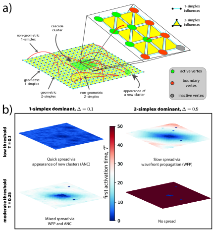
Figure 1: Local and non-local spreading patterns for a simplicial threshold model (STM) for cascades. a)  We initialize a STM cascade near the center of a two-dimensional (2D) noisy geometric complex, which contains both short-range geometric $k$-simplices and long-range non-geometric $k$-simplices. In this example, we study the clique complex kaczynski2004computational associated with a spatial graph in which vertices are arranged in $30\times 30$ triangular lattice (yielding a “geometrical substrate” comprised of vertices and geometric 1- and 2-simplices) and non-geometric edges are added uniformly at random (yielding a “topological noise” that manifest by non-geometric $k$-simplices in the clique complex).STM cascades can propagate by either local wavefront propagation (WFP) over a geometrical substrate or non-locally over non-geometric simplices to yield appearances of new clusters (ANC). Propagation to any boundary vertex $v_{i}$—which is inactive but has active simplicial neighbors (i.e., adjacent 1-simplices, 2-simplices, etc)—requires that the total activity across its simplicial neighbors (which can be aggregated in different ways) surpasses a threshold $T$. b)  We study 2D STM cascades that utilizes $k$-simplices with dimension $k\leq\kappa=2$, the relative interaction strength of 2-simplices versus 1-simplices is tuned by a parameter $\Delta\in[0,1]$ (see Eq. (2)). We depict the influence of $T$ and $\Delta$ on cascades’ spatio-temporal patterns by visualizing the activation times $\tau_{i}$ at which each vertex $v_{i}$ first becomes active. When $T$ and $\Delta$ are both small (top-left subpanel), STM cascades rapidly progress via ANC, yielding a ‘splotchy’ pattern. Increasing either $T$ or $\Delta$ suppresses ANC, thereby robustly guiding cascades along a geometrical substrate despite the presence of non-geometric $k$-simplices. (Observe in the bottom-right subpanel that STM cascades won’t spread if $T$ and/or $\Delta$ are too large.) In summary, multidimensional interactions and thresholding can coordinate to direct how and where cascades spread, which has implications for neuronal avalanches and other spatio-temporal cascades. See Section ‘Simplicial cascades robustly follow geometrical substrates and channels’ for further experiment details.

Our work is especially motivated by the study of cascading neuronal activity in brains shew2011information ; larremore2011predicting ; shew2013functional , since it is well-known that such dynamics involves both thresholding and higher-order interactions Yu17514 ; reimann2017cliques . Nevertheless, it has not been explored whether these two dynamical features coordinate in a nonlinear way to benefit brain function or play a role in orchestrating the propagation paths for brain activity. As an initial step in this direction, we study STM cascades over a simplicial complex model for a C. elegans synapse network Choe-2004-connectivity ; Kaiser-2006-placement in which pairwise edges represent neuronal synapses, and we use higher-order $k$-simplices in a simplicial complex to encode $(k+1)$-dimensional nonlinear dependencies (e.g., co-activations) among neurons reimann2017cliques . We refer to this model as a “neuronal complex,” and our experiments reveal that higher-order interactions promote the diversity and energy efficiency of STM cascades over the C. elegans neuronal complex. We emphasize that our findings for STM cascades are obtained for a model that we define to be intentionally simple so as to isolate and study nonlinear interplay between thresholding and higher-order coupling. Therefore, it remains unknown whether similar phenomena arise for biological networks of neurons and if our findings/methodologies can extend to more bio-realistic neuron models (e.g., Hodgkin–Huxley neurons brette2007simulation ). Nevertheless, our findings provide an important baseline of understanding for how higher-order interactions can potentially help orchestrate the spatio-temporal propagation of cascades over a neuronal network.

We support these findings with bifurcation theory to characterize WFP and ANC for STM cascades spreading over $k$-dimensional channels, which we define as a geometrical substrate comprised of $k$-simplices that extends in one dimension, thereby generalizing the graph-based notion of a ‘path’ to the setting of simplicial complexes. Our theory relies on a combinatorial analysis that considers the various possible dynamical responses for boundary vertices, which have simplicial neighbors that are active, but they themselves are not yet active. We also introduce simplicial cascade maps that attribute simplicial complexes with a latent geometry in which pairwise distances reflect the time required for STM cascades to travel between vertices. Simplicial cascade maps are a simplicial-complex generalization of contagion maps taylor2015topological , and they may similarly be used to quantitatively study the competition between WFP and ANC using techniques from high-dimensional data analysis, nonlinear-dimension reduction, manifold learning, and topological data analysis. Our proposed mathematical tools and computational experiments reveal that the multidimensional geometry of simplicial complexes can coordinate with the nonlinear propagation mechanism of thresholding to robustly orchestrate higher-order cascades, which is a promising direction for uncovering the multiscale, multidimensional mechanisms that facilitate higher-order information processing in neuro-systems, and more broadly, that determine the spatio-temporal patterns of cascades across other social, biological, and technological systems.

II Results

II.1 Simplicial threshold model (STM) for cascades

We first briefly describe simplicial complexes kaczynski2004computational . Consider a set $\mathcal{C}_{0}=\{v_{1},\dots,v_{N}\}$ of $N$ vertices. Each vertex $v_{i}\in\mathcal{C}_{0}$ is assigned a coordinate ${\bf y}^{(i)}\in\mathbb{R}^{p}$ in a $p$-dimensional ambient metric space. (We note in passing that vertices in “abstract” simplicial complexes do not have such coordinates; however, we will focus on the traditional definition herein.) We assume a Euclidean metric, although it may also be advantageous to explore other metric spaces krioukov2010hyperbolic ; boguna2021network . We can define a $k$-dimensional simplex $(v_{0},\dots,v_{k})$, or simply $k$-simplex, by an unordered set of vertices $v_{i}$ with cardinality $k+1$. For example, a $0$-simplex is equivalent to a vertex $v_{i}$ and a 1-simplex is equivalent to an undirected, unweighted edge $(v_{i},v_{j})$. Lastly, we define a $K$-dimensional simplicial complex $\{\mathcal{C}_{k}\}_{k=0}^{K}$ as the union of sets $\mathcal{C}_{k}$, each of which contain simplices of dimension $k$. For example, a 1-dimensional (1D) simplicial complex is a graph $\{\mathcal{C}_{k}\}_{k=0}^{1}$, where $\mathcal{C}_{0}$ is a set of vertices having spatial coordinates and $\mathcal{C}_{1}$ is a set of undirected, unweighted edges. Intuitively, a 2-dimensional simplicial complex is a spatial graph with “filled in” triangles. To define our cascade model, we further define notions of degree, or connectivity, among $k$-simplices. For each vertex $v_{i}\in\mathcal{C}_{0}$, we define $d_{i}^{k}$ as the number of $k$-simplices to which it is adjacent: $d_{i}^{1}$ is the 1-simplex degree of vertex $v_{i}$ (often called node degree for graphs), $d_{i}^{2}$ is its 2-simplex degree, and so on. We also define for each vertex $v_{i}$ the sets $\mathcal{N}^{k}(i)=\{s\in\mathcal{C}_{k}|i\in s\}$ that contain its $k$-dimensional simplicial neighbors. It follows that $d^{k}_{i}=|\mathcal{N}^{k}(i)|$ for each vertex $v_{i}$ and simplex dimension $k$.

We now define STM cascades in which all $k$-simplices of dimension $k\leq\kappa$ are given binary dynamical states $x_{i}^{k}(t)\in\{0,1\}$, i.e., inactive vs active, where index $i$ enumerates the simplices of dimension $k$ and $t\geq 0$ is time. For 2-dimensional (2D) STM cascades (i.e., $\kappa=2$), the states of vertices, 1-simplices, and 2-simplices are given by $\{x_{i}^{0}(t)\}$, $\{x_{i}^{1}(t)\}$, and $\{x_{i}^{2}(t)\}$, respectively. Parameter $\kappa$ is called the STM cascade’s dimension, and it may differ from that of the simplicial complex as long as $\kappa\leq K$. For $k>0$, the states of $k$-simplices are directly determined by the states of vertices; a $k$-simplex $(v_{0},\dots,v_{k})$ is active only when $k$ of the vertices are active. For example, an edge $(v_{i},v_{j})$ is active if at least one vertex $v_{i}$ or $v_{j}$ is active, a 2-simplex is active if at least two vertices are active, and so on. See Fig. 2a) for a visualization of states for vertices, 1-simplices, 2-simplices, and 3-simplices. We present these examples from the perspective of a boundary vertex, which we define as a vertex that is inactive but has at least one active simplicial neighbor.

The vertices’ states evolve via a discrete-time process that we define for general $\kappa$ in Methods section ‘STM cascades’. Here, we present a simplified dynamics for 2D STM cascades, and our later simulations will also focus on $\kappa=2$. At time step $t+1$, the state $x_{i}^{0}(t)$ of each vertex $v_{i}$ possibly changes according to a threshold criterion

$$x_{i}^{0}({t+1})=\left\{\begin{array}[]{rcl}1,&&\text{ if either }x_{i}^{0}({t})=1\text{ or }R_{i}({t})>T_{i}\,,\\ 0,&&\text{ if }x_{i}^{0}({t})=0\text{ and }R_{i}({t})\leq T_{i}\,,\end{array}\right.$$ (1)

where $T_{i}$ is an activation threshold intrinsic to vertex $v_{i}$ and

$$R_{i}({t})=(1-\Delta)f_{i}^{1}({t})+\Delta~{}f_{i}^{2}({t})$$ (2)

is a weighted average of cascade activity across the simplicial neighbors of vertex $v_{i}$. Parameter $\Delta$ tunes the relative influence of 2-simplices and $f_{i}^{1}(t)=\frac{1}{d^{1}_{i}}\sum_{j\in\mathcal{N}_{A}^{1}(i,t)}x_{j}^{1}(t)$ and $f_{i}^{2}(t)=\frac{1}{d^{2}_{i}}\sum_{j\in\mathcal{N}_{A}^{2}(i,t)}x_{j}^{2}(t)$ are the fractions of adjacent $1$- and $2$-simplices that are active at time $t$. One can also interpret $R_{i}({t})$ as $v_{i}$’s “simplicial exposure” to a cascade at time $t$. When vertices change their states, we allow $k$-simplices with $k>0$ to update their states instantaneously, and we leave open the investigation of more complicated dependencies such as delayed state changes for higher-dimensional $k$-simplices. Also, note that the limit $\Delta\to 0$ yields a 1D STM cascade, which is equivalent to the Watts threshold model Watts5766 for cascades over graphs.

To narrow the scope of our experiments, herein we initialize all STM cascades at time $t=0$ using cluster seeding (see Methods section ‘Cluster seeding’), in which case we select a vertex and set all of its adjacent vertices to be active, while all other vertices are inactive. Thresholding can potentially prevent localized initial conditions from propagating into large-scale cascades, and cluster seeding helps overcome this dynamical barrier gleeson2007seed ; taylor2015topological . Our experiments are also simplified by assuming an identical threshold $T_{i}=T$ for each vertex $v_{i}$. This allows us to explore the cooperative effects of thresholding and higher-order interactions for 2D STM cascades by varying only two parameters: threshold $T$ and 2-simplex influence $\Delta$.

Notably, we also define and study a stochastic variant of STM cascades in Supplementary Note ‘Stochastic Simplicial Threshold Model’ in which the vertices’ states change via a nonlinear stochastic process instead of the deterministic nonlinear dynamics defined by Eqs. (1)–(2).

Figure 2: Wavefront propagation (WFP) for $\kappa$-dimensional STM cascades on noisy ring complexes. a)  Each $k$-simplex with $k\leq\kappa$ is given a binary state $x_{i}^{k}(t)\in\{0,1\}$ indicating whether it is inactive or active, respectively, at time $t=0,1,2,\dots$. Cascade propagation occurs when an inactive boundary vertex is adjacent to sufficiently many active $k$-simplices, in which case it (and possibly some of its adjacent $k$-simplex neighbors) will become active upon the next time step. There are different types of inactive $k$-simplices, depending on how many of their vertices are active. b)  Noisy ring complexes (see Methods section ‘Generative model for noisy ring complexes’) generalize noisy ring lattices taylor2015topological and contain vertices that lie on a 1D ring manifold that is embedded in a 2D ‘ambient’ space. Each vertex has $d^{(NG)}=1$ non-geometric edge (red lines) to a distant vertex and $d^{(G)}$ geometric edges (blue lines) to nearby vertices with $d^{(G)}\in\{2,4,6\}$ (left, middle, and right columns, respectively). Higher-dimensional simplices arise in the associated clique complexes and are similarly classified as geometric/non-geometric. To simplify our illustrations, we place vertices alongside the manifold when $d^{(G)}>2$, and we do not visualize $3$-simplices. c)  Geometric $k$-simplices with $k\leq K$ compose a $K$-dimensional geometrical substrate. For noisy ring complexes, $K=d^{(G)}/2$ and the substrate is a $K$-dimensional channel—which is a non-intersecting sequence of lower-adjacent $K$-simplices. Channels generalize the graph-theoretic notion of a ‘path’. d)  STM cascades with different dimension $\kappa\leq K$ can propagate by WFP along a $K$-dimensional channel. Note that an STM cascade does not utilize all available $k$-simplices when $\kappa<K$.

II.2 Noisy geometric complexes, geometrical substrates and channels

We study the spatio-temporal patterns of STM cascades over noisy geometric complexes, which contain both short- and long-range simplices and are a generalization of noisy geometric networks taylor2015topological . Short- and long-range interactions have been observed in a wide variety of applications (e.g., face-to-face and online interactions in social networks) and are known to play an important structural/dynamical role for neuronal activity roxin2004self ; percha2005transition . It’s also worth noting that noisy geometric networks exhibit the small-world property watts1998collective under certain parameter choices, and noisy geometric complexes will likely exhibit a simplicial analogue to this property klamt2009hypergraphs ; bolle2006thermodynamics .

To explore WFP and ANC in an analytically tractable setting, we assume that the vertices $\mathcal{C}_{0}$ lie along a manifold within an ambient space $\mathbb{R}^{p}$, and that all $k$-simplices are one of two types: geometric simplices that connect vertices that are nearby on the manifold, and long-range non-geometric simplices that connect distant vertices. Each $k$-simplex is considered to be geometric if and only if all of its associated faces are geometric. After categorizing $k$-simplices as geometric or non-geometric, we further refine the notion of $k$-simplex degrees. Specifically, we let $d^{k,G}_{i}$ and $d^{k,NG}_{i}$ denote geometric and non-geometric $k$-simplex degrees, respectively, of a vertex $v_{i}$ so that $d^{k}_{i}=d^{k,G}_{i}+d^{k,NG}_{i}$. We provide visualizations of synthetic examples of noisy geometric complexes in Fig. 1 and Fig. 2b), where the vertices lie on a 2D plane and a 1D ring manifold, respectively. In these synthetic models, we construct geometric edges by connecting each vertex to several of its nearest neighbors, and we create non-geometric edges uniformly at random between pairs of vertices that do not yet have an edge. In either case, we construct noisy geometric complexes by considering the associated clique complexes for these vertices and edges. See Methods section ‘Generative model for noisy ring complexes’ for further details about this construction.

We define the subgraph (or sub-complex) restricted to geometric edges (or simplices) as a geometrical substrate, and propagation along a substrate is called WFP, by definition. Importantly, a substrate’s geometry and dimensionality can in principle differ from that of the manifold and that of the full simplicial complex that contains both geometric and non-geometric edges. For example, in Fig. 2b) we depict three noisy ring complexes in which the vertices have different geometric degrees: $d^{(G)}\in\{2,4,6\}$. In all cases, the vertices lie on a 1D ring manifold that is embedded in a 2D ambient space; however, as shown in Fig. 2c), the resulting $K$-dimensional geometrical substrates have different dimensions with $K=d^{(G)}/2$. Because each substrate extends in 1 dimension along the 1D ring manifold, each is a $K$-dimensional geometrical channel, which we define as a non-intersecting sequence of lower-adjacent $K$-simplices (i.e., each subsequent $K$-simplex intersects with the preceding $K$-simplex by a $(K-1)$-simplex that is a face to both $K$-simplices kaczynski2004computational ). A channel is a higher-dimensional generalization of a “non-intersecting path” in a graph in which wavefronts travel the fastest, and it is closely related to the graph-based concepts of $k$-clique rolling derenyi2005clique and complex paths guilbeault2021topological .

Before continuing, we highlight that it is important to understand the different types of ‘dimension’ that have been introduced. We assume that a noisy geometric complex lies on a manifold of some dimension and is within a $p$-dimensional metric space. The dimension $K$ of a simplicial complex refers to the maximum dimension of its $k$-simplices. Within a given simplicial complex, there can exist a geometrical substrate of some possibly smaller dimension $k$. Finally a STM cascade has its own dimension, $\kappa$, which is the largest $k$-simplex dimension that is utilized by the nonlinear dynamics. In principle, all of these dimensions can differ.

II.3 Simplicial cascades robustly follow geometrical substrates and channels

We study the coordinated effects of thresholding and higher-order interactions on WFP and ANC, and it is helpful to first provide precise definitions of these two phenomena that manifest as a frustration between local and non-local connections in a noisy geometric complex. We characterize a propagation to a vertex as WFP if at the time of propagation, it is adjacent to at least one active vertex via a geometric $k$-simplex. In contrast, a propagation to a vertex is called ANC if and only if that propagation occurs solely due to its adjacency to non-geometric active $k$-simplices, and all of its adjacent geometric $k$-simplices are inactive at the time of propagation.

Thresholding and higher-order interactions can both suppress non-local ANC across non-geometric edges, which promotes simplicial cascades to locally propagate via WFP along a geometrical substrate. This is visualized in Fig. 1, where we study 2D STM cascades over a 2D noisy geometric complex (The manifold, simplicial complex, geometrical substrate, and STM cascades all have the same dimension in this simple example.). We initialized the STM cascades with cluster seeding at a center vertex so that they could potentially spread outward via WFP along the 2D manifold (which is discretized by the geometrical substrate). In Fig. 1b), we visualize the activation times $\tau_{i}$ (i.e., when each vertex $v_{i}$ first becomes active), showing results for STM cascades with four choices for the parameters $T$ and $\Delta$. We study 2D STM cascades over a 2D noisy geometric complex in which the vertices are positioned in a $30\times 30$ triangular lattice, and each vertex $v_{i}$ has $d_{i}^{1,G}=6$ geometric edges to nearest neighbors (although vertices on the outside have fewer) as well as $d_{i}^{1,NG}=1$ non-geometric edge, which are added uniformly at random between pairs of vertices. We then study the resulting clique complex. Observe for small $T$ and $\Delta$ (top-left subpanel) that STM cascades rapidly spread and predominantly exhibit ANC, which results in the ‘splotchy’ pattern. In contrast, when either $T$ or $\Delta$ is increased, the simplicial cascade predominantly exhibits WFP, and not ANC, which slows propagation and enables the cascade to more reliably follow along the geometrical substrate (i.e., thereby overcoming the presence of long-range “topological noise”). Finally, observe that if $T$ and $\Delta$ are too large (bottom-right subpanel), then the initial seed cluster does not lead to a cascade.

This finding extends existing knowledge about the effects of short- and long-range connections on cascades. It is well-known that long-range edges allow traditional pairwise-progressing cascades to rapidly spread via the mechanism of ANC. This concept is most apparent in the context of epidemic spreading, and as a response, banning international airline travel is often a first response to prevent long-range transmissions for epidemics hollingsworth2006will ; epstein2007controlling ; colizza2007modeling . However, ANC is also suppressed when the cascade’s propagation mechanism requires a vertex’s neighboring activity (i.e., ‘exposure’) to surpass a threshold $T$ centola2007cascade ; centola2007complex ; centola2010spread ; taylor2015topological ; mahler2021analysis . We find that higher-order interactions can be as, if not more, effective at suppressing non-local ANC. Moreover, these two mechanisms can coordinate to more robustly guide cascades along a geometrical substrate despite the presence of topological (i.e., non-geometric) noise. In the next sections, we explore the potential benefits of this structural/dynamical coordination as a multiscale/multidimensional mechanism to orchestrate neuronal avalanches.

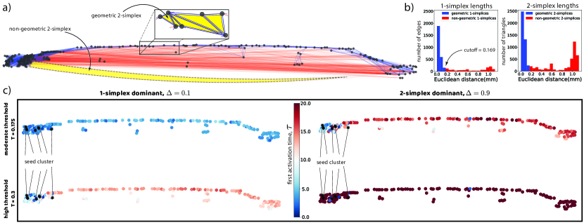
Figure 3: STM cascades on a C. elegans neuronal complex. a) 2D visualization of experimentally measured locations and synapse connections between neurons in nematode C. elegans Choe-2004-connectivity ; Kaiser-2006-placement . We model higher-order nonlinear dynamical dependencies among sets of $(k+1)$ neurons using $k$-simplices in the associated clique complex for which we ignore edge directions. b) Histograms depict the distribution of lengths for 1- and 2-simplices, where we define the length of a 2-simplex as the maximum length over its faces. We distinguish geometric and non-geometric $1$-simplices by selecting a cutoff distance of 0.169 mm, and we characterize a 2-simplex as geometric if and only if all of its faces are geometric. c) Vertex colors depict their first-activation times $\tau_{i}$ for a 2D STM cascade that is initialized with the indicated seed cluster. Observe that $T$ and $\Delta$ affect the spatio-temporal pattern of activations (i.e., WFP and ANC) similarly to what was shown in Fig. 1a).

II.4 STM cascades on a C. elegans neuronal complex

We observe similar cooperative effects of thresholding and higher-order interactions for STM cascades on a neuronal complex, which we define as a simplicial complex model that represents the higher-order nonlinear interdependencies between neurons. We study simplicial cascades over a neuronal complex representation for the neural circuitry and dynamics for nematode C. elegans Choe-2004-connectivity ; Kaiser-2006-placement . In this example, vertices represent neurons’ somas (i.e., cell bodies), edges represent experimentally observed synapses, and we use higher-order simplices to encode potential higher-order nonlinear dynamical relationships (e.g., co-activations) between combinatorial sets of neurons reimann2017cliques . Notably, we simulate STM cascades on an undirected C. elegans synapse network since our model and theory doesn’t involve directed $k$-simplices.

In Fig. 3a), we visualize the C. elegans neuronal complex. The locations of vertices reflect experimental measurements for the somas’ centers. The length of each edge gives the distance between somas, which we use as an estimate for the combined lengths of the axon and dendrite involved in each synapse. Geometric and non-geometric edges are indicated by blue and red lines, respectively. For simplicity, we do not visualize higher-dimensional simplices. We provide a histogram of edge lengths in Fig. 3b), and observe that most edges are short-range, but there are also many long-range connections. We heuristically classify edges as geometric/non-geometric depending on whether edge lengths are less than or greater than a “cutoff” distance of 0.169 mm. Note that this choice of threshold has no effect on the dynamics of STM cascades. Finally, we construct a neuronal complex by considering the graph’s associated clique complex kaczynski2004computational .

Observe that the C. elegans neuronal complex approximately lies on a 1D manifold that is embedded 2D, which occurs due to the elongated shape of a nematode worm. Thus, we are interested in understanding the extent to which simplicial cascades locally propagate by WFP along the 1D manifold versus non-local ANC. To provide insight, in Fig. 3c) we visualize first activation times $\tau_{i}$ for 2D STM cascades with different parameters $T$ and $\Delta$. These subpanels recapitulate our visualizations in Fig. 1b): thresholding and higher-order interactions both suppress non-local ANC and can cooperatively promote WFP along a geometrical substrate or channel. (We will support this quantitatively below.)

While our knowledge of neuronal cascades has grown immensely in recent years luczak ; beggsetal ; shew2011information ; shew2013functional ; larremore2011predicting , the mathematical mechanisms responsible for directing where and how cascades propagate have remained elusive. The coordination of higher-order nonlinear thresholding and the multidimensional geometry of simplicial complexes is a plausible structural/dynamical mechanism that can help self-organize neuronal cascades. Of course, the combined effects of other dynamical features (e.g., refractory periods, inhibition, and stochasticity brette2007simulation ) should also be explored. In particular, neurons are known to exhibit alternating states of polarization/depolarization. In contrast, the STM cascades that we study here involve irreversible state transitions as a way to a baseline of understanding for the interplay between thresholding and higher-order interactions in the absence of the confounding effects of other dynamical features. As an initial step toward generalising STM cascades, we provide extended experiments in Supplementary Note ‘Stochastic Simplicial Threshold Model.’ Nevertheless, our work highlights this emerging field as a promising direction for unveiling the multiscale mechanisms that orchestrate higher-order information processing within, but not limited to, neuronal systems.

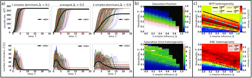
Figure 4: Higher-order interactions enhance diversity and efficiency for STM cascade patterns on a C. elegans neuronal complex. a)  Cascade size $q(t)$ (top) and the number $C(t)$ of spatially disjoint clusters (bottom) versus time $t$ for 2D STM cascades with threshold $T=0.1$ and $\Delta\in\{0.1,0.5,0.9\}$. Different curves represent different initial conditions, and black curves give their means. b)  For STM cascades with different $T$ and $\Delta$, colors indicate (top) the fraction $\phi$ of initial conditions in which a cascade saturates the neuronal complex (i.e., spreads everywhere) and (bottom) the standard deviation $\sigma$ of the times at which saturations occur. Black regions indicate $(T,\Delta)$ values for which no cascades saturate the network. Cascades are most heterogeneous when $T$ and $\Delta$ are neither too small or large. c)  Colors indicate the heterogeneity of WFP and ANC properties by showing (top) $h(\{q(t)\})$ and (bottom) $h(\{C(t)\})$, where $h(\cdot)$ denotes the discrete Shannon entropy of a set of cascades with different initial conditions (see Methods section ‘Entropy Calculation’). We focus on time $t=5$, since these measures are most reflective of WFP and ANC at early times. Lines indicate bifurcation theory that we will develop for STM cascades over noisy ring lattices, but as can be seen, the theory is also qualitatively predictive for this neuronal complex. Observe that increasing $\Delta$ causes the spatio-temporal patterns’ changes (i.e., bifurcations) to occur for smaller $T$ values, which lowers the energy consumption per neuron activation.

II.5 Higher-order interactions enhance patterns’ diversity and efficiency

Higher-order interactions promote heterogeneity for STM cascades’ spatio-temporal patterns, which has important implications in the context of neuronal cascades. Specifically, neuronal networks that exhibit more ‘expressive’ activity patterns have broader memory capacity shew2011information ; shew2013functional , which has been shown to occur for neuronal networks that are tuned near ‘criticality’—i.e., a dynamical phase transition. At the same time, there is extensive empirical evidence that neuron interactions are higher-order Yu17514 ; reimann2017cliques , yet mathematical theory development for neuronal cascades has largely remained limited to dyadic-interaction models (see, e.g., larremore2011predicting ).

Motivated by these insights, here we study the diversity and efficiency for STM cascades over the C. elegans neuronal complex. In Fig. 4, we study how parameters $T$ and $\Delta$ effect the heterogeneity of STM cascades. In Fig. 4a), we study WFP (top) and ANC (bottom) properties by plotting the cascade size $q(t)$ and the number of clusters $C(t)$, respectively, as STM cascades propagate. The left, center, and right columns show results for STM cascades that are 1-simplex dominant ($\Delta=0.1$), averaged ($\Delta=0.5$) and 2-simplex dominant ($\Delta=0.9$), respectively. In each subpanel, different curves represent different initial conditions, whereby we select different vertices to initiate cluster seeding. Black curves indicate the means across initial conditions. Observe that some STM cascades spread to the entire neuronal complex and are said to saturate the network, whereas others do not. Also, early on, the numbers of clusters increase due to ANC, but they can later decrease as cascade clusters grow and merge. Moreover, there is significant heterogeneity across the different cascades’ initializations, which arises due to the heterogeneous connectivity of neurons within the neuronal complex. This heterogeneity becomes more prominent as $\Delta$ (the 2-simplex influence) increases.

In Fig. 4b), we further study cascade heterogeneity for different initial conditions and different choices for $T$ and $\Delta$. We plot (top) the fraction $\phi$ of cascades that saturate the network (i.e., when all vertices become active) and (bottom) the standard deviation $\sigma$ for the times at which saturations occur. The black-colored regions highlight that no STM cascades saturate the network if $T$ and/or $\Delta$ are too large. Observe that the cascades’ saturation fractions and times are most heterogeneous when $T$ and $\Delta$ are neither too small nor too large. This suggests thresholding and higher-order interactions may also play a ‘critical’ role for helping tune neuronal networks to exhibit maximal cascade pattern diversity (which is called ‘wide dynamic range’ when considered from a multiscale perspective).

In Fig. 4c), we focus on $q(t)$ and $C(t)$ when $t=5$, which is an early time in which these values provide empirical quantitative measures for WFP and ANC, respectively. (At larger times $t$, it is difficult to distinguish WFP and ANC propagations since the cascades are so large.) For different $T$ and $\Delta$, we study the heterogeneity of these values by computing the Shannon entropy of (top) $h(\{q(t)\})$ and (bottom) $h(\{C(t)\})$ across the different initial conditions. See Methods section ‘Entropy Calculation’ for details. Observe that the entropy of cascade sizes is largest when $T$ and $\Delta$ are neither too small or too large, which is similar to our finding in Fig. 4b). When considering $h(\{C(t)\})$, we do not observe a similar peak for intermediate values of $T$ and $\Delta$; however the changes in entropy for $C(t)$ and $q(t)$ occur at approximately the same values of $T$ and $\Delta$, since the spatio-temporal patterns (i.e., ANC and WFP) undergo changes at these particular parameter choices.

We further highlight in Figs. 4b) and 4c) that as $\Delta$ increases, the dynamical changes can be observed to occur at smaller values of $T$. This has important implications for the efficiency of STM cascades. Specifically, we define the ‘activation energy’ of a vertex to equal the minimum fraction of active vertices that are required in order for that vertex to become active. For our model, a vertex’s activation energy monotonically decreases as $T$ decreases, since fewer neighboring activations are be required to overcome a smaller threshold barrier. In other words, a small threshold would allow a cascade to propagate efficiently, with each vertex’s activation requiring the activation of only a small number of other vertex activations.

However, it can also be important that a threshold $T$ allows cascades with different initial conditions to produce heterogeneous cascade patterns. Our experimental results in Fig. 4b) and 4c) have shown that increasing the 2-simplex influence $\Delta$ shifts the phase transitions for dynamical behavior to occur for smaller $T$ values. In other words, the introduction of higher-order interactions for these experiments allows cascades with similarly complex patterns to occur for smaller $T$ values (i.e., when their activation energies are smaller).

As a concrete example, consider our visualization of $h(\{q(t)\})$ in in Fig. 4c), which is given by the Shannon entropy of cascade sizes at time $t=5$ across all initial conditions with cluster seeding. For each $\Delta$, we can consider the threshold $T$ at which $h(\{q(t)\})$ are most heterogeneous. For $\Delta\approx 0$, $h(\{q(t)\})$ obtains its maximum near $T=0.25$, but for $\Delta\approx 1$, $h(\{q(t)\})$ obtains its maximum near $T=0.1$ (i.e., when vertices have a smaller activation energy). In both cases, the maximum is approximately $h(\{q(5)\})\approx 2.8$. In this way, the presence of higher-order interactions allows cascade patterns with similarly complexity to be produced more efficiently.

Finally, by considering STM cascades across the $(T,\Delta)$ parameter space, we can systematically investigate the complementary effects of thresholding and higher-order interactions. We will develop bifurcation theory in the next section to guide this exploration, which is represented by the solid and dashed lines in Fig. 4c). Importantly, our theory will be developed for STM cascades over the family of noisy ring complexes that we presented in Methods section ‘Generative model for noisy ring complexes’, and as such, it is not guaranteed to be predictive for other simplicial complexes. That said, one can remarkably observe in Fig. 4c) that this theory is qualitatively predictive for C. elegans neuronal complex.

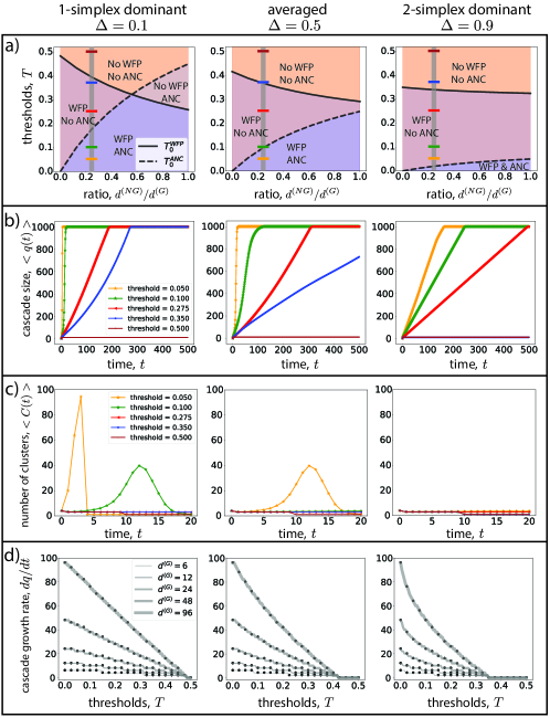
Figure 5: Bifurcation theory characterizes WFP and ANC over $K$-dimensional geometrical channels. We consider 2D STM cascades over a noisy ring complex (recall Fig. 2) for various $T$ and either (left) $\Delta=0.1$, (center) $\Delta=0.5$, or (right) $\Delta=0.9$. a)  Bifurcation diagrams depict the critical thresholds $T_{0}^{WFP}$ and $T_{0}^{ANC}$ given by Eqs. (3) and (4), respectively, for different $T$, $d^{(NG)}$ and $d^{(G)}$. We find four regimes that are characterized by the absence/presence of WFP and ANC. Observe that increasing $\Delta$ suppresses ANC, and the regime that exhibits ANC with no WFP disappears under higher-order coupling with $\Delta>0.1$. Vertical gray lines and horizontal colored marks identify the values $d^{(NG)}/d^{(G)}=0.25$ and $T\in\{0.05,0.1,0.275,0.35,0.5\}$, and in panels b) and c) we show for these values that the spatio-temporal patterns of STM cascades are as predicted. b)  Colored curves indicate the sizes $q(t)$ of STM cascades versus time $t$, averaged across all possible initial conditions with cluster seeding. c)  Colored curves indicate the average number $C(t)$ of cascade clusters, and one can observe a peak only when ANC occurs. Three scenarios give rise to WFP and ANC: $(\Delta,T)\in\{(0.1,0.05),(0.1,0.1),(0.5,0.05)\}$. Four scenarios give rise to no spreading: $(\Delta,T)\in\{(0.1,0.5),(0.5,0.5),(0.9,0.35),(0.9,0.5)\}$. The other selected values of $\Delta$ and $T$ yield WFP and no ANC, in which case $q(t)$ grows linearly, $dq/dt=2(j+1)$ for $T\in[T^{WFP}_{j+1},T^{WFP}_{j})$. d)  Black symbols and gray curves indicate observed and predicted values, respectively, of cascade growth rates, $dq/dt$, for STM cascades exhibiting WFP and no ANC for a noisy ring complex with $d^{(NG)}=0$ and $d^{(G)}\in\{6,12,24,48,96\}$ (i.e., channel dimensions $K\in\{3,6,12,24,48\}$). Combining high-dimensional channels with higher-order interactions allows cascade growth rates to have a nonlinear sensitivity to changes for the threshold $T$.

II.6 Bifurcation theory for STM Cascades over geometrical channels

We analyze WFP and ANC for STM cascades over a family of simplicial complexes in which $N$ vertices lie along a 1D manifold as shown in Fig. 2b), and for which the vertices’ degrees lack heterogeneity (although our experiments highlight that the theory can be qualitatively predictive beyond this assumption). See Methods section ‘Generative model for noisy ring complexes’ for their formation, which generalizes the noisy ring lattices that are studied in taylor2015topological , wherein the authors developed bifurcation theory to predict WFP and ANC properties for a threshold-based cascade model that is restricted to dyadic interactions. In the Methods section ‘Combinatorial analysis for bifurcation theory’ we describe bifurcation theory that characterizes STM cascades over noisy ring complexes. We present general theory for $\kappa$-dimensional STM cascades, and we summarize here bifurcation theory for 2D STM cascades. Our theory assumes large $N$ and is based on a combinatorial analysis for the different possible state changes for boundary vertices that have active simplicial neighbors, but they themselves are not yet active. We focus on the early stage of cascades in which they are just beginning to spread, and we summarize our results below.

Our primary findings are two sequences of critical thresholds that characterize WFP and ANC and which depend on the STM parameter $\Delta$ and degrees $d^{(G)}$, $d^{(NG)}$, $d_{i}^{1}$, and $d_{i}^{2}$. The qualitative properties of WFP are determined by critical thresholds

$$T^{WFP}_{j}=(1-\Delta)\frac{s_{j}}{d_{i}^{1}}+\Delta\frac{1}{d_{i}^{2}}\binom{s_{j}}{2},$$ (3)

where $s_{j}={d^{(G)}}/{2}-j$ is the number of active geometric 1-simplex neighbors and $j\in\{0,1,..,{d^{(G)}}/{2}\}$. The first and second terms in Eq. (3) represent 1-simplex and 2-simplex influences, respectively. Here, we highlight that $\binom{s_{j}}{2}$ equals the number of geometric 2-simplex neighbors that are active, since we assume that for every pair of active geometric 1-simplex neighbors of $v_{i}$, there exists an associated geometric 2-simplex neighbor of $v_{i}$. This is true for the geometric substrate for which we develop theory, which is a clique complex associated with geometric edges that are arranged in a $k$-regular ring lattice. While the thresholds $T^{WFP}_{j}$ may differ for vertices $v_{i}$ that have different $k$-simplex degrees, they are the same for simplicial complexes that are “$k$-simplex degree-regular” and have identical local connectivity in the geometric substrate. Moreover, Eq. (3) has assumed that non-geometric $k$-simplices are inactive, which occurs with very high probability for small cascades in which $q(t)/N\ll 1$. The resulting critical thresholds identify ranges $T\in[T^{WFP}_{j+1},T^{WFP}_{j})$ such that the speed of WFP is identical for any threshold $T$ within a given range. Within each range, the WFP speed is $j+1$. For noisy ring complexes, WFP progresses in the clockwise and counter-clockwise directions, given the cascade growth $q(t)\approx(2j+2)t$ for small $t$. There is no WFP when $T>T^{WFP}_{0}$.

Similarly, the qualitative properties of ANC are determined by critical thresholds

$$T^{ANC}_{j}=(1-\Delta)\frac{d^{(NG)}-j}{d_{i}^{1}},$$ (4)

where $j\in\{0,1,..,d^{(NG)}\}$ and $d^{(NG)}-j$ represents the number of adjacent non-geometric 1-simplices that are active. Note that there is not a second term in the right-hand side of Eq. (4), since our theory assumes that the non-geometric 2-simplex neighbors of a vertex $v_{i}$ are inactive at early cascade times (i.e., small $t$). Such an event occurs with vanishing probability when $q(t)/N$ is small. Also note that Eq. (4) assumes all geometric neighbors are inactive, which is required by the definition of ANC. It follows that the probability of ANC occurrences is the same for any $T\in[T^{ANC}_{j+1},T^{ANC}_{j})$, and it is different for any two $T$ values in different regions. Notably, there is no ANC if $T>T^{ANC}_{0}$.

In Fig. 5a), we show bifurcation diagrams that characterize WFP and ANC for different choices of $T$ and the ratio $d^{(NG)}/d^{(G)}$. Solid and dashed black lines indicate $T^{WFP}_{0}$ and $T^{ANC}_{0}$, respectively. Different columns depict bifurcation diagrams for different STM cascades that are either: (left, $\Delta=0.1$) 1-simplex dominant; (center, $\Delta=0.5$) averaged; or (right, $\Delta=0.9$) 2-simplex dominant. The vertical gray lines and horizontal colored marks indicate choices for the ratio $d^{(NG)}/d^{(G)}$ and $T$ that are further studied in Figs. 5b) and 5c). Observe in Fig. 5a) that as $\Delta$ increases, the region of parameter space exhibiting WFP and no ANC expands, whereas the region exhibiting WFP and ANC shrinks. Notably, the region exhibiting ANC and no WFP vanishes altogether for $\Delta>0.1$. In other word, as STM cascades are more strongly influenced by higher-order interactions, they exhibit an increase in WFP and a decrease in ANC; they more robustly propagate via WFP along a geometrical channel/substrate, and they are less impacted by the ‘topological noise’ that is imposed by the presence of long-range, non-geometric $k$-simplices.

In Figs. 5b) and 5c), we plot the cascade size $q(t)$ and number $C(t)$ of clusters, respectively, as a function time $t$. These are averaged across all possible initial conditions with cluster seeding. As before, the left, center and right columns depict the choices $\Delta\in\{0.1,0.5,0.9\}$. In each panel, we show several curves for different thresholds $T\in\{0.05,0.1,0.275,0.37,0.5\}$. All panels reflect results for noisy ring complexes with $d^{(G)}=8$ and $d^{(NG)}=2$ (i.e., $d^{(NG)}/d^{(G)}=0.25$). Our selection for these parameter choices was guided by the bifurcation diagrams in Fig. 5a). We chose these particular values to highlight the impact of $\Delta$ and $T$ on WFP and ANC properties. In particular, cascades exhibiting WFP and no ANC will have linear growth for $q(t)$ and the number of clusters $C(t)$ does not increase. (Note that it would be quadratic growth for WFP on the 2D manifold shown in Fig. 1, cubic growth for 3D manifolds, and so on.) On the other hand, cascades exhibiting WFP and ANC will have very rapid growth for $q(t)$ and an initial spike for the number of clusters $C(t)$. $C(t)$ can later decrease as clusters merge together. Finally, cascades do not spread if they neither exhibit WFP nor ANC.

One can observe in Figs. 5b) and 5c) that the qualitative features of WFP and ANC occur for different choices of $T$ and $\Delta$ exactly as predicted by our bifurcation theory. First, there is no spreading when $T=0.5$ and $\Delta\in\{0.1,0.5\}$ (left and center columns), or when $T\in\{0.35,0.5\}$ and $\Delta=0.9$ (right column), since $T>T_{0}^{WFP}$ and $T>T_{0}^{ANC}$ in these cases and there is neither WFP nor ANC. Second, there is a sharp rise in the number of clusters and rapid, super-linear growth only when $T\in\{0.05,0.1\}$ and $\Delta=0.1$ (left column) and when $T=0.05$ with $\Delta=0.5$ (center column), since $T<T_{0}^{WFP}$ and $T<T_{0}^{ANC}$ in these cases and both WFP and ANC occur. Third, for all other values of $T$ and $\Delta$, the curves exhibit linear growth when $t$ is small, since $T<T_{0}^{WFP}$ and $T>T_{0}^{ANC}$ and there is WFP but no ANC. (The growth rate of spreading can be faster at later times $t$, since our bifurcation theory focuses on the nature of spreading dynamics at early stages of the cascades.)

In Fig. 5d), we study how the speed of WFP along a geometric channel is affected by the threshold $T$, 2-simplex influence parameter $\Delta$, and the channel dimension $K=d^{(G)}/2$. Black symbols and gray curves indicate observed and predicted values of cascade growth size, $dq/dt$, for $d^{(NG)}=0$ and different choices of $d^{(G)}\in\{6,12,24,48,96\}$. First, observe that our prediction $dq/dt=2(j+1)$ for $T\in[T^{WFP}_{j+1},T^{WFP}_{j})$ is very accurate for the different parameter values. Second, observe that ${dq}/{dt}$ generally increases with the channel dimension $K$. Lastly, observe in the right column of Fig. 5d) that by introducing higher-order interactions (i.e., large $\Delta$), cascade growth rates ${dq}/{dt}$ have a nonlinear sensitivity to changes of the threshold $T$. Such a nonlinear response could benefit the directing of cascade propagation via mechanisms that modulate activation thresholds (e.g., neurochemical modulations).

In Fig. 6, we study how increasing either $T$ or $\Delta$ generically slows the spread of STM cascades, and in particular, it slows the rates of both WFP and ANC behaviors. This is predicted by the other critical thresholds given in Eqs. (3) and (4) for different values of $j\geq 0$. In Fig. 6a), we use color to depict the average rate of change for $q(t)$ at time $t=5$, which is an empirical measure for WFP speed. We predict linear growth for $q(t)$ at a rate of ${dq}/{dt}\approx 2j+2$ for $T\in[T^{WFP}_{j+1},T^{WFP}_{j})$, which is very close to what we empirically observe. Observe that as $\Delta$ increases, the ranges associated with larger $j$ broaden, whereas the ranges associated with smaller $j$ narrow. This can be understood by examining the right-hand side of Eq. (3) and noting that the first term is linear, whereas the second term is combinatorial. Hence, as STM cascades are more strongly influenced by 2-simplex interactions, slower WFP becomes a more dominant phenomenon across the $T$-parameter space.

In Fig. 6b), we use color to depict the average number $C(t)$ of clusters at time $t=5$, which is an empirical measure for the rate of ANC. Our bifurcation theory predicts three ranges $T\in[T^{ANC}_{j+1},T^{ANC}_{j})$, and as expected, the observed number of clusters is similar within these ranges and different across them. Importantly, increasing $\Delta$ causes all of the thresholds $T_{j}^{ANC}$ to approach 0. Thus, for any fixed $T$, increasing $\Delta$ will cause ANC events to vanish altogether. So while thresholding and higher-order interactions play a similar mechanistic role in that they both suppress ANC and allow WFP, higher-order interactions achieve this much more effectively.

In Figs. 6d) and 6e), we depict similar information as Figs. 6a) and 6b), except it is computed for the C. elegans neuronal complex, rather than a noisy ring complex for which the bifurcation theory was developed. See Methods section ‘Critical Regimes for C. elegans’ for further information. Despite being outside the assumptions of our bifurcation theory, Eqs. (3) and (4) surprisingly predictive for the qualitative behavior of WFP and ANC for the C. elegans neuronal complex (that is, spatio-temporal pattern changes still occur near the bifurcation lines). Also, observe that the transitions in Figs. 6d) and 6e) are not as abrupt as those shown in Figs. 6a) and 6b), since the neuronal complex has heterogeneous 1- and 2-simplex degrees, which is known to blur bifurcation taylor2015topological . Nevertheless, the theory accurately predicts the general trend for how increasing $\Delta$ leads to a suppression of ANC, thereby promoting WFP.

In Supplementary Note “Effects of 1-Simplex Degree Heterogeneity on STM Cascades”, we numerically study how heterogeneity added to the geometric and/or non-geometric 1-simplex degrees affects bifurcations that occur for WFP and ANC for 2D STM cascades over noisy ring complexes. Our main finding is that our analytically derived bifurcations remain qualitatively accurate even when a small amount of degree heterogeneity is introduced. We also find that the introduction of heterogeneity for non-geometric edges decreases the range of $T$ for which WFP is predominantly exhibited over ANC. Interestingly, increasing the influence of 2-simplices (i.e., increasing $\Delta$) counterbalances this effect. That is, higher-order interactions help simplicial cascades become more robust to the noise imposed by degree heterogeneity (see Supplementary Figure 6, lower row). In Supplementary Material Section ‘Effects of 2-simplex degree heterogeneity on STM cascades,’ we further extend this study, finding that the introduction of significant irregularity into a geometric substrate can significantly reduce WFP; however, the introduction of many non-geometric $2$-simplices has comparatively little effect on STM cascades for early times in which $q(t)$ is small.

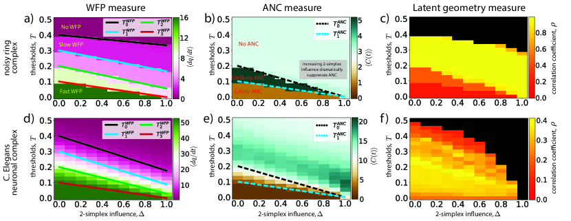
Figure 6: Empirical measurements for WFP and ANC rates predicted by critical thresholds $T_{j}^{WFP}$ and $T_{j}^{ANC}$. We study 2D STM cascades with various $T$ and $\Delta$ over (top row) a noisy ring complex with $N=1000$ vertices, $d^{(G)}=8$, and $d^{(NG)}=2$ and (bottom row) the C. elegans neuronal complex. a)  An empirical measure for WFP speed, $\frac{dq}{dt}$, which we compute at $t=5$ and average across all initial conditions with cluster seeding. Observe that $\frac{dq}{dt}$ undergoes changes at the critical thresholds $T_{j}^{WFP}$ given by Eq. (3), which vary with $\Delta$. Within each region $T\in[T_{j+1}^{WFP},T_{j}^{WFP})$, observe that the growth rate is close to our predicted rate of $2j+2$. b)  An empirical measure for ANC, $C(t)$, which we compute at $t=5$ and average across initial conditions. Observe that $C(t)$ undergoes changes that are accurately predicted by critical thresholds $T_{j}^{ANC}$ given in Eq. (4). That is, there are three regions $T\in[T_{j+1}^{ANC},T_{j}^{ANC})$, and ANC events occur at approximately the same rate within each region. c)  A Pearson correlation coefficient $\rho$ quantifies the extent to which STM cascades predominantly follow along the manifold via WFP. It is computed by comparing pairwise-distances between vertices $v_{i}$ to $v_{i^{\prime}}$ in the original 2D ambient space containing the ring manifold to pairwise-distances $||\bm{\tau}^{(i)}-\bm{\tau}^{(j)}||_{2}$ between a nonlinear embedding of $N$ vertices $v_{i}$ and $v_{j}$ using STM Cascade Maps $\{i\}\mapsto\{\bm{\tau}^{(i)}\}\in\mathbb{R}^{J}$ for which distances reflect the time required for STM cascades to travel between vertices (see Methods section ‘Simplicial cascade maps’). d)–f)  Similar information as in panels a)–c), except for the C. elegans neuronal complex.

II.7 Latent geometry of simplicial cascades quantifies WFP vs ANC

It was proposed in taylor2015topological to quantitatively study competition between WFP and ANC using techniques from high-dimensional data analysis, nonlinear dimension reduction, manifold learning, and topological data analysis. The approach relied on constructing “contagion maps” in which a set of vertices $\mathcal{C}_{0}$ in a graph are nonlinearly embedded in a Euclidean metric space so that the distances between vertices reflect the time required for contagions to traverse between them. Contagion maps are similar to other nonlinear embeddings that are based on diffusion coifman2006diffusion and shortest-path distance tenenbaum2000global , but in contrast, they provide insights about the dynamics of thresholded cascades (as opposed to the dynamics of heat diffusion, for example). We generalize this approach by attributing the vertices in a simplicial complex with a latent geometry so that pairwise distances between vertices reflect the time required for STM cascades to traverse between them. See Methods section ‘Simplicial cascade maps’ for details on this construction. Each cascade map uses $J$ different initial conditions with cluster seeding to yield a point cloud $\{v_{i}\}\mapsto\{\bm{\tau}^{(i)}\}\in\mathbb{R}^{J}$. For each, we compute the Pearson correlation coefficient $\rho$ between pairwise distances $||\bm{\tau}^{(i)}-\bm{\tau}^{(j)}||_{2}$ in the latent embedding and pairwise distances between vertices in the original ambient space (e.g., locations on a ring manifold in 2D or the empirically observed locations of somas for C. elegans). See Supplementary Note “Visualizations of STM Cascade Maps” for visualizations of these point clouds and further discussion.

In Figs. 6c) and 6f), we use the high-dimensional geometry of simplicial cascade maps to quantitatively study the competing phenomena for WFP and ANC for a noisy ring complex and the C. elegans neuronal complex, respectively. We use color to visualize $\rho$ for different simplicial cascade maps using STM cascades with different choices for $\Delta$ and $T$. Larger values of $\rho$ indicate parameter choices in which cascades exhibit a prevalence of WFP versus ANC, whereas smaller $\rho$ indicate the opposite. Observe in both Figs. 6c) and 6f) that larger $\rho$ values occur for an intermediate regime in which $T$ and $\Delta$ are neither too larger nor too small. In this regime, the geometry of simplicial cascade maps best matches the original 2D geometry, which occurs because STM cascades predominantly exhibit WFP along the geometrical substrate and are not disrupted by ANC across long-range simplices (i.e., the topological ‘noise’). By comparing the panels in Fig. 6c) to those in Figs. 6a) and 6b), observe that the regions of larger $\rho$ coincide with regions in which there is slow WFP and unlikely ANC, as is predicted by our bifurcation theory. Finally, observe that the $\rho$ values are generally larger for the noisy ring complex than for the C. elegans complex. This likely occurs because the noisy ring complexes that we study have no degree heterogeneity, whereas the C. elegans neuronal complex does have heterogeneous $k$-simplex degrees. Also, we note that the C. elegans neuronal complex contains many more non-geometric 2-simplices than that of the noisy ring complexes. That said, our extended experiments in Supplementary Material Section ‘Effects of 2-simplex degree heterogeneity on STM cascades’ suggest that it is the irregularity of geometric $k$-simplices—not the non-geometric $k$-simplices—that has the greatest impact on WFP and ANC.

III Discussion

Nonlinear cascades arise in diverse types of social, biological, physical and technological systems, many of which are insufficiently represented by cascade models that are restricted to pairwise (i.e., dyadic) interactions james2016information ; Yu17514 ; maclean ; mayfield ; ghasemi2021data ; dass2011holistic ; lanchier2013stochastic ; civilini2021evolutionary ; noonan2021dynamics ; patania . Thus motivated, we have proposed a simplicial threshold model (STM) for cascades over simplicial complexes that encode dyadic, triadic, and higher-order interactions. Our work complements recent higher-order models for epidemic spreading bodo2016sis ; petrietal ; barratetal ; chowdaryetal ; restrepoetal ; PhysRevResearch.2.012049 ; higham2021epidemics , social contagions PhysRevResearch.2.023032 ; neuhauser2021opinion , and consensus yu2011distributed ; neuhauser2020multibody ; neuhauser2021consensus ; sahasrabuddhe2021modelling , and in particular, the effects of higher-order interactions on spatio-temporal patterns (i.e., WFP vs ANC) and the implications for neuronal avalanches have not yet been explored. By assigning the states of active/inactive to individual vertices as well as groups of vertices, STM cascades provide a new modeling framework that can help bridge individual-based threshold models (e.g., social contagions and neuron interactions) with group-based threshold models (e.g., group decision making and interacting neuron groups such as cortical columns or structural communities). In particular, simplicial cascades allow for the modeling of “multidimensional cascades” in which the states of individuals influence the states of groups, and vice versa, and such interactions cannot be appropriately represented by graph-based modeling. Herein, the dynamical states of higher-dimensional simplices are inherited by their associated vertices’ states, and it would be interesting in future work to explore more complicated dependencies such as allowing time lags between when a vertex becomes active and when its adjacent higher-dimensional simplices subsequently become active. Such multidimensional models remain an exciting open avenue for research.

By studying STM cascades over “noisy geometric complexes”—a family of spatially embedded simplicial complexes that contain both short- and long-range $k$-simplices—our work reveals the interplay between higher-order dynamical nonlinearity and the multidimensional geometry of simplicial complexes to be a promising direction for research into how complex systems organize the spatio-temporal patterns of cascade dynamics. We have shown that the coordination of higher-order coupling and thresholding allows STM cascades to robustly suppress the appearance of new clusters (ANC), yielding local wavefront propagation (WFP) along a geometrical substrate. STM cascades can propagate along $k$-dimensional geometrical channels (i.e., a sequence of “lower adjacent” $k$-simplices) despite the presence of long-range simplices (which introduce a “topological noise” to the geometry). While taylor2015topological ; mahler2021analysis presents bifurcation theory describing how thresholding impacts WFP and ANC on noisy geometric networks containing short- and long-range edges, no prior work has explored the effects of higher-order coupling on WFP and ANC. This is problematic, since understanding whether a cascade predominantly spreads locally or non-locally significantly impacts the steps that one takes, e.g., to predict and control cascades onnela2010spontaneous ; bentley2021social ; hollingsworth2006will ; epstein2007controlling ; colizza2007modeling ; gu2015controllability ; medaglia2020personalizing ; dobson2007complex ; hines2016cascading ; pathak2007complexity ; dolgui2018ripple ; mari2015adaptivity . Our bifurcation theory for STM cascades over geometrical channels (see Fig. 2 and Eqs. (3) and (4)) was shown to accurately predict how WFP and ANC change depending on parameters of the cascade (i.e., threshold $T$ and a parameter $\Delta$ that tunes the relative strength of 2-simplex interactions) and parameters of the noisy geometric complex (i.e., the $k$-simplex degrees, which measure the number of number of geometric edges, $d^{(G)}$, non-geometric edges, $d^{(NG)}$, and 2-simplices, $d^{2}$, that are adjacent to a vertex). This theory characterizes the absence/presence of WFP and ANC and their respective rates, and it provides a solid theoretical foundation to support the exploration of WFP and ANC for higher-order cascades in a variety applied settings (e.g., neuronal avalanches, cascading failures, and so on).

Our work provides important insights for higher-order information processing in neuronal networks and other complex systems. Higher-order dependencies are widely observed for neuronal activity Yu17514 ; reimann2017cliques , yet theory development for neuronal cascades is largely restricted to pairwise-interaction models larremore2011predicting . Thus motivated, we studied STM cascades over a ‘neuronal complex’ that represents the structural and higher-order nonlinear dynamical dependencies among neurons in nematode C. elegans. We have shown that thresholding and higher-order interactions can collectively orchestrate the spatio-temporal patterns of STM cascades that spread across the multidimensional geometry of a neuronal complex, which we predict to be an important mathematical mechanism that can potentially help brains direct neuronal cascades and optimize the diversity and efficiency of cascades’ spatio-temporal patterns (see Fig. 4). Given the importance of efficiency in brains, simplicial-complex modeling is expected to also lead to new perspectives for other types of efficiency, such as wiring efficiency sporns . Moreover, we have shown (see Fig. 2d)) that the combination of higher-order coupling with high-dimensional channels allows the growth-rates of STM cascades to be nonlinearly sensitive to changes in $T$, which may benefit the directing of multiscale cascades via the (e.g., neurochemical) modulation of activation thresholds $T_{i}$. Moreover, the sizes and durations of neuronal avalanches are known to exhibit wide dynamical range shew2011information ; larremore2011predicting ; shew2013functional , and we have shown that higher-order interactions can provide a mechanism for growth rates to have similar heavy-tailed heterogeneity (which we pose as a measurable hypothesis for the neuroscience community).

It is also worth noting that we have proposed an intentionally simple model for higher-order cascades with the goal of gaining concrete, analytically tractable insights. Future work should investigate the combined effects of other dynamical properties of neurons (e.g., alternating states of activity/inactivity, refractory periods, inhibition, directed edges, and stochasticity brette2007simulation ) and other dynamical behaviors such as local/non-local patterns for synchronized neuron firings (which may benefit from recent advances in synchronization theory for higher-order systems PhysRevLett.124.218301 ; PhysRevResearch.2.023281 ; gambuzzaetal ; calmon2021topological ; skardal2021higher ). In this same vein, future research should also investigate biological processes that could possibly mediate the coordination of higher-order interactions and thresholding, particularly by incorporating empirical neuronal data. Thus motivated, we introduce and study a stochastic variant of STM cascades in Supplementary Note ‘Stochastic Simplicial Threshold Model’. We show that our results for deterministic STM cascades remain qualitatively similar as long as the propagation mechanism remains dominated by thresholding and not stochasticity.

Finally, we have introduced a technique called ‘simplicial cascade maps’ that embed a simplicial complex in a latent metric space. This nonlinear embedding extends contagion maps taylor2015topological , which are recovered under the assumption of 1D STM cascades, and both mappings embed vertices so that the distance between vertices reflects how long cascades take to traverse from one vertex to another. Simplicial cascade maps generalize the well-developed field of graph embedding to the context of simplicial complexes, and we have used them to quantitatively study the extent to which STM cascades follow geometrical channels within a simplicial complex, i.e., as opposed to exhibiting non-local ANC phenomena. Although it is not our focus herein, simplicial cascade maps are expected to support higher-order generalizations of methodology development for manifold learning, topological data analysis, and nonlinear dimension reduction. Notably, STM cascades can robustly follow geometrical substrate despite the presence of topological noise, which is a property that can benefit these data-science pursuits when they are applied to noisy data.

IV Methods

IV.1 STM cascades

In the text above, we focused on the case of 2D STM cascades. We now define a general version for STM cascades of dimension $\kappa\geq 1$. At time step $t+1$, the state $x_{i}^{0}(t)$ of each vertex $v_{i}$ possibly changes according to the threshold criterion given by Eq. (2) except that we now define the simplicial exposure to be

$$R_{i}^{t}=\sum_{k=1}^{\kappa}\alpha_{k}f_{i}^{k}(t),$$ (5)

where $f_{i}^{k}(t)=\frac{1}{d^{k}_{i}}\sum_{j\in\mathcal{N}_{A}^{k}(i)}x_{j}^{k}(t)$ is the fraction of vertex $v_{i}$’s neighboring $k$-simplices that are active and $\{\alpha_{k}\}$ are non-negative weights that satisfy $1=\sum_{k}\alpha_{k}$. The choice $\alpha_{1}=(1-\Delta)$, $\alpha_{2}=\Delta$ and $\kappa=2$ recovers the model for 2D STM cascades that we studied above. In Supplementary Note ‘Stochastic Stochastic Simplicial Threshold Model’, we formulate and study a stochastic generalization of this model.

IV.2 Cluster seeding

We initialize an STM cascade at a vertex $v_{i}$ with cluster seeding, which we define as follows. Let $\mathcal{N}^{1}(i)\subset\mathcal{C}_{0}$ denote the set of vertices that are adjacent to $v_{i}$ through $1$-simplices. We set $x_{j}^{0}(0)=1$ for any $j\in\mathcal{N}^{1}(i)$ at time $t=0$ and $x_{j^{\prime}}^{0}(0)=0$ for any $j^{\prime}\not\in\mathcal{N}^{1}(i)$. Thus, the size of an STM cascade at time $t=0$ is $q(0)=d_{i}^{1}$, which can possibly vary depending on the vertex degrees. Note that the seed vertex $v_{i}$ itself is not in the set $\mathcal{N}^{1}(i)$, since we assume no self loops. Therefore $x_{i}^{0}(0)$ is inactive at $t=0$, but it will very likely become active at time $t=1$ (excluding the situation of pathologically large $\Delta$ and $T$).

IV.3 Generative model for noisy ring complexes

We construct noisy ring complexes by considering the clique complexes associated with noisy ring lattices taylor2015topological . First, we place $N$ vertices $v_{i}$ at angles $\theta_{i}=2\pi(i/N)$ for $i\in\{1,\dots,N\}$. We then create geometric edges by connecting each vertex to its $d^{(G)}$ nearest neighbors. We assume $d^{(G)}$ to be an even number so that ${d^{(G)}}/{2}$ edges go in either direction along the 1D manifold. Next, we create non-geometric edges uniformly at random between the vertices so that each vertex has exactly $d^{(NG)}$ non-geometric edges. We generate non-geometric edges using the configuration model, except we introduce a re-sampling procedure to avoid adding an edge that already exists. The resulting graph is a noisy ring lattice, and we construct its associated clique complex to yield a noisy ring complex. (Recall that a clique complex is a simplicial complex that is derived from a graph, and there is a one-to-one correspondence between each clique involving $(k+1)$ vertices in the graph and each $k$-simplex in the simplicial complex.) Finally, each $k$-simplex is then defined to be geometric or non-geometric, depending on whether it involves one or more non-geometric edge. This generative model yields noisy ring complexes that are specified by three parameters: $N$, $d^{(G)}$ and $d^{(NG)}$.

Noisy ring complexes are particularly amenable to theory development because they are degree regular with respect to the 1-simplex degrees; each vertex $v_{i}$ is adjacent to exactly $d_{i}^{1}=d^{(G)}+d^{(NG)}$ 1-simplices, where $d^{(G)}$ and $d^{(NG)}$ are the geometric and non-geometric 1-simplex degrees, respectively. The degrees $d_{i}^{k}$ of higher-order simplices are not degree regular; however, the geometric degrees $d_{i}^{k,G}$ for $k\geq 1$ are identical across vertices due to the symmetry of the geometrical substrate (i.e., the ‘sub’ simplicial complex that includes only geometric simplices).

While STM cascades can be studied over any simplicial complex, we focus herein on clique complexes, which helps facilitate the identification of adjacencies among $k$-simplices. If ${\bf A}$ is a graph’s adjacency matrix so that $A_{ij}=1$ if $(v_{i},v_{j})\in\mathcal{C}_{1}$ and $A_{ij}=0$ otherwise, then an entry $B_{ij}$ in matrix ${\bf B}={\bf A}^{2}*{\bf A}$ encodes the number of 2-simplices that are shared by vertices $v_{i}$ and $v_{j}$. (Here, $*$ denotes the Haddamard, or ‘entrywise’, product.) In this work, we make use of matrices ${\bf A}$ and ${\bf B}$ when numerically implementing 2D STM cascades over clique complexes.

IV.4 Entropy calculation

We use Shannon entropy in Fig. 4c) to quantify the diversity of spatio-temporal patterns of 2D STM cascades on a C. elegans neuronal complex, and we compute it as follows. In each panel of Fig. 4a), we plot (top) cascade size $q(t)$ and (bottom) the number of spatially distant cascade clusters $C(t)$, and different curves indicate $q(t)$ and $C(t)$ for different initial conditions with cluster seeding. Focusing on $t=5$, we consider the sets $\{q(5)\}$ and $\{C(5)\}$ and approximate their probability distributions by constructing histograms with $20$ bins. Letting $p_{i}$ denote the fraction of entries that fall into the $i$-th bin, we compute the associated discrete Shannon entropy

$$h=-\sum_{i=1}^{20}p_{i}\log{p_{i}}.$$ (6)

We note that our choice for the number of bins does effect the total entropy; however, we find that it has little effect on the qualitative behavior for how heterogeneity changes across the $(T,\Delta)$ parameter space, which is our main interest for Fig. 4c).

IV.5 Combinatorial analysis for bifurcation theory

We now present the derivation of our bifurcation theory given in Eqs. (3) and (4) for 2D STM cascades over noisy ring complexes. Recall for this model that $N$ nodes are positioned along a the unit circle and are spaced apart by an angle $\delta=2\pi/N$. Therefore, neighboring vertices are positioned apart by angles $1\delta$, $2\delta$, and so on. Also, recall that each vertex has exactly $d^{(G)}$ geometric edges to nearest-neighbor vertices and $d^{(NG)}$ non-geometric edges to other vertices, which are added uniformly at random. This generative model for noisy geometric complexes helps us to develop theory for ANC and WFP, but as we shall show, it also has important implications for such phenomena.

We first describe ANC in the limit of large $N$ when the cascade size $q(t)$ is small. By definition, an ANC event occurs when a cascade propagates to a vertex $v_{i}$ that is far from a cascade cluster, implying that all of its geometric $k$-simplices are inactive. It follows that the fractions of active adjacent $k$-simplices can only take on the following values

$$f^{k}_{i}\in\left\{0,\frac{1}{d_{i}^{k}},\frac{2}{d_{i}^{k}},\dots,\frac{d_{i}^{k,NG}}{d_{i}^{k}}\right\},$$ (7)

depending on the number of active non-geometric $k$-simplices. For STM cascades over noisy ring complexes that are generated via the model that we describe in Methods section ‘Generative model for noisy ring complexes’, we find that ANC events occur predominantly due to influences by non-geometric 1-simplices. In contrast, we find non-geometric 2-simplices to have a negligible effect on ANC in the limit of large $N$, small $q(t)$, and fixed $d^{(G)}$ and $d^{(NG)}$, which implies $f^{2}_{i}\approx 0$ under these assumptions. Specifically, non-geometric 2-simplices (and higher-dimensional simplices) are rare, because non-geometric edges are added uniformly at random. Consider a vertex $v_{i}$ that is distant from a cascade cluster, and suppose that it has one non-geometric edge to an active vertex $v_{j}$. That edge is the face of a 2-simplex only if $v_{i}$ has a second non-geometric edge to a third vertex that is already adjacent to $v_{j}$. This occurs with probability $1-[(N-1-d^{1}_{i})/N]^{(d^{(NG)}-1)}\sim\mathcal{O}({N}^{-1})$, which approaches zero with increasing $N$. This result uses that there are $N-1-d^{1}_{i}$ possible vertices that $v_{i}$ can connect to without creating a non-geometric 2-simplex $v_{j}$. Since non-geometric edges are created uniformly at random, each of the remaining non-geometric edges for $v_{i}$ don’t create a 2-simplex with probability $[(N-1-d^{1}_{i})/N]$. Moreover, $[(N-1-d^{1}_{i})/N]^{(d^{(NG)}-1)}$ gives the probability that none of them do. Subtracting this probability by 1 gives the probability that there is at least one non-geometric 2-simplex between $v_{i}$ and $v_{j}$ (that is, given that they are already connected by a non-geometric edge). Therefore, while non-geometric 2-simplices (and higher-dimensional simplices) do arise in our generative model for noisy ring complexes, they are rare and have little effect on ANC for large systems.

To obtain the critical thresholds given in Eq. (4), we approximate $R_{i}(t)\approx(1-\Delta)f^{1}_{i}$ and observe that

$$f^{1}_{i}\in\left\{0,\frac{1}{d^{(G)}+d^{(NG)}},\dots,\frac{d^{(NG)}}{d^{(G)}+d^{(NG)}}\right\},$$ (8)

which uses that the 1-simplices are degree regular. If one considers a variable threshold $T$, then the probability that ANC events occur will significantly change as $T$ surpasses the different $R_{i}(t)$ values corresponding to different $f^{1}_{i}$. For example, there are no ANC events when $T>(1-\Delta)\frac{d^{(NG)}}{d^{(G)}+d^{(NG)}}$.

Notably, our bifurcation theory for ANC naturally extends to $\kappa$-dimensional STM cascades in which $R_{i}(t)=\sum_{k=1}^{\kappa}\alpha_{k}f_{i}^{k}(t)$. In this case, non-geometric $k$-simplices with $k>1$ also have little effect on ANC, and the critical thresholds are identical to those in Eq. (4) with the variable substitution $(1-\Delta)\mapsto\alpha_{1}$.

We next develop bifurcation theory for WFP dynamics, and in this case, higher-dimensional simplices have a significant effect. Our analysis stems from considering boundary vertices that are not yet active but have geometric simplicial neighbors—i.e., adjacent geometric 1-simplices, geometric 2-simplices, etc.—that are active. The propagation speed of a wavefront along a geometrical channel is determined by the number of boundary vertices that become active upon each time step. For example, in Fig. 7a) we visualize a noisy ring complex with $d^{(G)}=6$ so that there are $d^{(G)}/2=3$ boundary vertices $\{v_{1},v_{2},v_{3}\}$ for the clockwise-progressing wavefront. (Recall that each vertex connects to $d^{(G)}/2$ nearest-neighbor vertices in either direction along the ring manifold.) Therefore, the speed of a wavefront is either 1, 2, or 3, depending on how many of them become active at each time step. Note that the cascade exposure $R_{i}(t)$ defined in Eq. (2) will be different for each boundary vertex, and because they are enumerated closest-to-farthest from the wavefront, one has $f_{1}^{k}(t)\geq f_{2}^{k}(t)\geq f_{3}^{k}(t)$ and $R_{1}(t)\geq R_{2}(t)\geq R_{3}(t)$. Therefore, as a threshold $T_{i}$ increases, the criterion $R_{i}(t)>T_{i}$ defined in Eq. (1) will first fail for $v_{3}$, then $v_{2}$, and finally $v_{1}$. The wavefront shown in Fig. 7 won’t propagate for any threshold that is larger than $R_{1}(t)$.

The $R_{i}(t)$ values of boundary vertices reveal critical threshold values for WFP, and we identify them for noisy ring complexes by considering how each $v_{i}$ is adjacent to geometric $k$-simplices that are either active or inactive. We may assume that the non-geometric $k$-simplices are inactive in the limit of large $N$ and small cascades size $q(t)$ [technically, a non-geometric $k$-simplex is active with probability that is at most $\mathcal{O}(q(t)/N)$], and so we initially focus on $d^{(NG)}=0$. We will later allow for nonzero $d^{(NG)}$ when we compute the fractions $f_{i}^{k}(t)$. To this end, we define for each $v_{i}$ the sets $\mathcal{N}^{k}(i)$ of adjacent $k$-simplices, which we partition into sets $\mathcal{N}_{A}^{k}(i,t)$ and $\mathcal{N}_{I}^{k}(i,t)$ of adjacent $k$-simplices that are active and inactive, respectively, at time $t$. Note that $\mathcal{N}^{k}(i)=\mathcal{N}_{A}^{k}(i,t)\cup\mathcal{N}_{I}^{k}(i,t)$ and $d^{k}_{i}=|\mathcal{N}^{k}(i)|$ is the degree of $v_{i}$ with respect to $k$-simplices. With these definitions, the fractions of active $k$-simplices are given by

$$f_{i}^{k}(t)=\frac{|\mathcal{N}_{A}^{k}(i,t)|}{d_{i}^{k}}.$$ (9)

In Fig. 7b), we visualize a wavefront propagating along a geometrical channel for the noisy ring complex shown in Fig. 7a). Vertices are positioned so that we may more easily identify whether $2$-simplices are active or inactive. Focusing on the boundary vertex $v_{1}$ that is closest to the wavefront and has the largest exposure $R_{i}(t)$, we illustrate its set of adjacent 2-simplices that are active. Because $v_{1}$ is adjacent to $|\mathcal{N}_{A}^{1}(1,t)|=3$ active 1-simplices and $|\mathcal{N}_{A}^{2}(1,t)|=3$ active 2-simplices, it follows that $f_{1}^{1}(t)=\frac{3}{d_{i}^{1}}$ and $f_{1}^{2}(t)=\frac{3}{d_{i}^{2}}$. (Note that the denominators include both geometric and non-geometric $k$-simplices.) We also visualize in Fig. 7b) the inactive 2-simplices that are adjacent to boundary vertex $v_{1}$. Recall from Fig. 2 that there are two types of inactive 2-simplices, depending on whether a 2-simplex contains only one active vertex (type 1) or no active vertices (type 2). We let $\mathcal{N}^{2}_{I_{1}}(i,t)$ and $\mathcal{N}^{2}_{I_{2}}(i,t)$ denote the sets of inactive 2-simplices of types 1 and 2, respectively, and depict them for $v_{1}$. Observe that $|\mathcal{N}_{I}^{1}(1,t)|=|\mathcal{N}_{I_{1}}^{2}(1,t)|=|\mathcal{N}_{I_{2}}^{2}(1,t)|=3$.

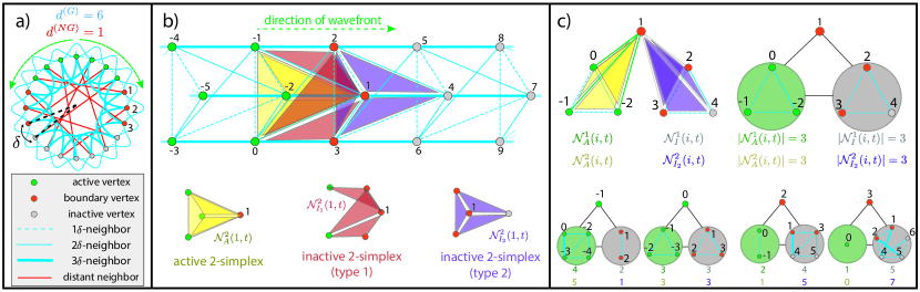
Figure 7: Bifurcation theory obtained by examining the connections between boundary vertices and active/inactive $1$- and $2$-simplices. a)  Visualization of a noisy ring complex with $d^{(G)}=6$ and $d^{(NG)}=1$ with $N$ vertices that are spaced apart by an angle $\delta=2\pi/N$. Linestyles highlight that edges connect neighbors with different proximity, and we label vertices so that vertex $v_{1}$ is positioned $1\delta$ to the right of the wavefront, $v_{2}$ is at position $2\delta$, and so on. The speed of WFP is determined by the number of boundary vertices $\{v_{1},v_{2},v_{3}\}$ that become active upon the next time step. b)  Visualization of active and inactive $k$-simplices for the boundary vertex $v_{1}$ that is closest to the wavefront. For each $v_{i}$, we define a set $\mathcal{N}_{A}^{k}(i,t)$ of adjacent $k$-simplices that are active and sets $\mathcal{N}_{I_{1}}^{k}(i,t)$ and $\mathcal{N}_{I_{2}}^{k}(i,t)$ of inactive 2-simplices that are type 1 and 2, respectively. (Recall Fig. 2.) c)  By identifying a set of neighboring active vertices (green shaded regions) for a boundary vertex $v_{i}$, one can compute the number of adjacent 1- and 2-simplices that are active by counting the number of those vertices and the number of edges among them, respectively. One can identify the number of inactive 1-simplices and type-2 inactive 2-simplices in a similar way (gray shaded regions). This approach is depicted for vertex $v_{1}$ (top) as well as other nearby vertices (bottom), and the associated numbers are indicated for each.

In Fig. 7c), we highlight that one can easily compute the number of active 1- and 2-simplices that are adjacent to a boundary vertex $v_{i}$ using three steps. First, we identify the set $\{v_{j}|(i,j)\in\mathcal{N}_{A}^{1}(i,t)\}$ of active vertices that are connected to $v_{i}$ by active 1-simplices (see green shaded regions). Second, we count the number of vertices in that set, which yields $|\mathcal{N}_{A}^{1}(i,t)|$ since there is a one-to-one correspondence between these vertices and the active 1-simplices that are adjacent to $v_{i}$. Third, we count the number of edges among those vertices, which yields $|\mathcal{N}_{A}^{2}(i,t)|$ since there is a one-to-one correspondence between those edges and active 2-simplices. We can also calculate the number of type-2 inactive 2-simplices in a similar way. That is, we first identify the set $\{v_{j}|(i,j)\in\mathcal{N}_{I}^{1}(i,t)\}$ of inactive vertices that are connected to $v_{i}$ by inactive 1-simplices (see gray shaded regions in Fig. 7c)). We then count how many vertices are in the set (which yields $|\mathcal{N}_{I}^{1}(i,t)|$) and the number of edges among those vertices (which yields $|\mathcal{N}_{I_{2}}^{2}(i,t)|$). The upper part of Fig. 7c) illustrates this approach for $v_{1}$, and we do not visualize type-1 inactive 2-simplices, because they are more difficult to compute directly but can be found after the other sets are determined: $|\mathcal{N}_{I_{1}}^{2}(i,t)|=d_{i}^{2}-|\mathcal{N}_{A}^{2}(i,t)|-|\mathcal{N}_{I_{2}}^{2}(i,t)|$. The lower part of Fig. 7c) illustrates this approach for the other two boundary vertices $\{v_{2},v_{3}\}$ as well as two vertices $\{v_{-1},v_{0}\}$ that are already active, since they are to the left of the wavefront.

Importantly, because each vertex has exactly $d^{(G)}/2$ 1-simplices going in either side along the ring manifold left, there is always a clique of edges among vertices in a set $\{v_{j}|(i,j)\in\mathcal{N}_{A}^{1}(i,t)\}$ for the boundary vertices. (This is not true for active vertices, such as $v_{-1}$, as shown in the lower part of Fig. 7c).) Therefore, if a boundary vertex has $s_{j}$ active 1-simplices, then it must also have $\binom{s_{j}}{2}$ active 2-simplices. It follows that the different possible $f_{i}^{1}$ values for a boundary vertex $v_{i}$ are given by

$$f^{1}_{i}\in\left\{0,\frac{1}{d^{1}_{i}},\frac{2}{d^{1}_{i}},\dots,\frac{d^{(G)/2}}{d^{1}_{i}}\right\},$$ (10)

and the corresponding $f_{i}^{2}$ values are

$$f^{2}_{i}\in\left\{0,\frac{1}{d^{2}_{i}}\binom{1}{2},\frac{1}{d^{2}_{i}}\binom{2}{2},\dots,\frac{1}{d^{2}_{i}}\binom{d^{(G)}/2}{2}\right\}.$$ (11)

We enumerate these possibilities by $j$ and use the definition $R_{i}(t)=(1-\Delta)f^{1}_{i}+\Delta f^{2}_{i}$ to obtain the critical threshold values for WFP given by Eq. (3). For $\kappa$-dimensional STM cascades, setting $T=R_{i}(t)$ yields a more general set of bifurcation lines:

$$T^{WFP}_{j}=\sum_{k=1}^{\kappa}\alpha_{k}\frac{1}{d_{i}^{2}}\binom{s_{j}^{(G)}}{k}.$$ (12)

In either case, $(j+1)$ boundary vertices will become active upon each time step when $T\in[T_{j+1}^{WFP},T_{j}^{WFP})$. Since wavefronts progress both clockwise and counter-clockwise around the ring manifold, the cascade size $q(t)$ will grow linearly at a rate $2j+2$.

IV.6 Critical regimes for C. elegans

Our bifurcation theory describes WFP and ANC on a 1D geometrical substrate is degree regular, so that STM cascade propagations occur identically for all boundary vertices. However, the empirical neuronal complex for C. elegans is degree heterogeneous, and so we instead examine the median bifurcation curves that are associated with median degrees, including geometric degrees, non-geometric degrees, and 2-simplex. In principle, we could plot a different bifurcation curve for each vertex $v_{i}$ based on its unique degrees. (See Supplementary Figure 9 and related discussion on ‘Perturbed Bifurcation Results’ in Supplementary Note 3 of taylor2015topological .) For simplicity, here we instead plot a single representative bifurcation curve for C. elegans using the median values $d^{(G)}=8$, $d^{(NG)}=2$, and $d^{2}=34$ to construct the bifurcation curves. Finally, we reiterate that the C. elegans neuronal complex has a structure that is outside our assumed structure of a noisy ring complex, and so our bifurcation theory should not be expected to be perfectly predictive. Our experiments highlight that these bifurcation curves are qualitatively predictive for the general effects of $T$ and $\Delta$.

IV.7 Simplicial cascade maps

We introduce a notion of latent geometry for simplicial complexes called simplicial cascade maps in which the set $\mathcal{C}_{0}=\{1,\dots,N\}$ of vertices is nonlinearly mapped as a set of points (i.e., a ‘point cloud’) in an $J$-dimensional Euclidean metric space $\mathbb{R}^{J}$. Simplicial cascade maps directly generalize contagion maps taylor2015topological , which are recovered under the choice of 1D STM cascades (and which do not utilize $k$-simplices for $k>1$).

We construct simplicial cascade maps using the activation times for STM cascades. Given $J$ realizations of a STM cascade on a simplicial complex with different initial conditions with cluster seeding, the associated STM map is a map $\{v_{i}\}\mapsto\{\bm{\tau}^{(i)}\}\in\mathbb{R}^{J}$ in which each vertex $v_{i}\in\mathcal{C}_{0}$ maps to a point $\bm{\tau}^{(i)}=[\tau^{(i)}_{1},\dots,\tau^{(i)}_{J}]^{T}$, where $\tau^{(i)}_{j}$ is the activation time for vertex $v_{i}$ for the STM cascade with the $j$-th initial condition. See Supplementary Note “Visualizations of STM Cascade Maps” for visualizations of these point clouds and further discussion.

In practice, we often let $J=N$ so that the $j$-th initial condition corresponds to seed clustering at vertex $v_{j}$. However, extra attention is required for handling cascades that don’t saturate the network, in which case there would be $\tau^{(i)}_{j}$ values that are undefined. Herein, we choose to neglect such cascades. See taylor2015topological for alternative strategies in the context of cascades over graphs.

IV.8 Data and code availability

The authors declare that all data supporting the findings of this study are available within the paper. A codebase that implements STM cascades over noisy geometric complexes and reproduces our computational experiments can be found in a Python library neuronal_cascades . Documentation on how to use this software is available at neuronal_cascades_doc . The C. elegans synapse network with physical vertex positions is publicly available and was downloaded from Kaiser-2011 ; data .

Author Contributions

Both authors developed the research plan and wrote the paper. BUK conducted the numerical experiments.

Competing Interests

The authors declare that there are no competing interests.

- [1] Alain Barrat, Guilherme Ferraz de Arruda, Iacopo Iacopini, and Yamir Moreno. Social contagion on higher-order structures. arXiv:2103.03709, 2021.
- [2] Marc Barthélemy. Spatial networks. Physics Reports, 499(1-3):1–101, 2011.
- [3] D. Bassett and ED Bullmore. Small-world brain networks. The Neuroscientist, 12(6):512–523, 2006.
- [4] Plenz D. Beggs JM. Neuronal avalanches in neocortical circuits. Journal of Neuroscience, 23(35):11167–1117, 2003.
- [5] Kara Bentley, Charlene Chu, Cristina Nistor, Ekin Pehlivan, and Taylan Yalcin. Social media engagement for global influencers. Journal of Global Marketing, pages 1–15, 2021.
- [6] J. Billings, M. Saggar, J. Hlinka, S. Keilholz, and G. Petri. Simplicial and topological descriptions of human brain dynamics. Network Neuroscience, 5(2):549–568, 2021.
- [7] Ágnes Bodó, Gyula Y Katona, and Péter L Simon. SIS epidemic propagation on hypergraphs. Bulletin of Mathematical Biology, 78(4):713–735, 2016.
- [8] Marian Boguna, Ivan Bonamassa, Manlio De Domenico, Shlomo Havlin, Dmitri Krioukov, and M Ángeles Serrano. Network geometry. Nature Reviews Physics, 3(2):114–135, 2021.
- [9] Désiré Bollé, Rob Heylen, and NS Skantzos. Thermodynamics of spin systems on small-world hypergraphs. Physical Review E, 74(5):056111, 2006.
- [10] Romain Brette, Michelle Rudolph, Ted Carnevale, Michael Hines, David Beeman, James M Bower, Markus Diesmann, Abigail Morrison, Philip H Goodman, Frederick C Harris, et al. Simulation of networks of spiking neurons: a review of tools and strategies. Journal of Computational Neuroscience, 23(3):349–398, 2007.
- [11] Dirk Brockmann and Dirk Helbing. The hidden geometry of complex, network-driven contagion phenomena. Science, 342(6164):1337–1342, 2013.
- [12] Charles D. Brummitt, Raissa M. D’Souza, and E. A. Leicht. Suppressing cascades of load in interdependent networks. Proceedings of the National Academy of Sciences, 109(12):E680–E689, 2012.
- [13] Paul G. et al. Buldyrev S., Parshani R. Catastrophic cascade of failures in interdependent networks. Nature, 464:1025–1028, 2010.
- [14] E. Bullmore and O. Sporns. The economy of brain network organization. Nature Review Neuroscience, 13:336–349, 2012.
- [15] Lucille Calmon, Juan G Restrepo, Joaquín J Torres, and Ginestra Bianconi. Topological synchronization: explosive transition and rhythmic phase. arXiv preprint arXiv:2107.05107, 2021.
- [16] Xu Can, Wang Xuebin, and Skardal Per Sebastian. Bifurcation analysis and structural stability of simplicial oscillator populations. Physical Review Research, 2:023281, Jun 2020.
- [17] Timoteo Carletti, Duccio Fanelli, and Renaud Lambiotte. Random walks and community detection in hypergraphs. Journal of Physics: Complexity, 2(1):015011, 2021.
- [18] Damon Centola. The spread of behavior in an online social network experiment. Science, 329(5996):1194–1197, 2010.
- [19] Damon Centola, Víctor M Eguíluz, and Michael W Macy. Cascade dynamics of complex propagation. Physica A: Statistical Mechanics and its Applications, 374(1):449–456, 2007.
- [20] Damon Centola and Michael Macy. Complex contagions and the weakness of long ties. American Journal of Sociology, 113(3):702–734, 2007.
- [21] MacLean JN Chambers B. Higher-order synaptic interactions coordinate dynamics in recurrent networks. PLoS Computational Biology, 12(8):e1005078., 2016.
- [22] Sandeep Chowdhary, Aanjaneya Kumar, Giulia Cencetti, Iacopo Iacopini, and Federico Battiston. Simplicial contagion in temporal higher-order networks. arXiv:2105.04455, 2021.
- [23] Andrea Civilini, Nejat Anbarci, and Vito Latora. Evolutionary game model of risk propensity in group decision making. arXiv preprint arXiv:2104.11270, 2021.
- [24] Ronald R Coifman and Stéphane Lafon. Diffusion maps. Applied and computational harmonic analysis, 21(1):5–30, 2006.
- [25] Vittoria Colizza, Alain Barrat, Marc Barthelemy, Alain-Jacques Valleron, and Alessandro Vespignani. Modeling the worldwide spread of pandemic influenza: baseline case and containment interventions. PLoS Medicine, 4(1):e13, 2007.
- [26] Mayukh Dass and Gavin L Fox. A holistic network model for supply chain analysis. International Journal of Production Economics, 131(2):587–594, 2011.
- [27] de Arruda Guilherme Ferraz, Petri Giovanni, and Moreno Yamir. Social contagion models on hypergraphs. Physical Review Research, 2:023032, Apr 2020.
- [28] Imre Derényi, Gergely Palla, and Tamás Vicsek. Clique percolation in random networks. Physical Review Letters, 94(16):160202, 2005.
- [29] Ian Dobson, Benjamin A Carreras, Vickie E Lynch, and David E Newman. Complex systems analysis of series of blackouts: Cascading failure, critical points, and self-organization. Chaos: An Interdisciplinary Journal of Nonlinear Science, 17(2):026103, 2007.
- [30] Alexandre Dolgui, Dmitry Ivanov, and Boris Sokolov. Ripple effect in the supply chain: an analysis and recent literature. International Journal of Production Research, 56(1-2):414–430, 2018.
- [31] Joshua M Epstein, D Michael Goedecke, Feng Yu, Robert J Morris, Diane K Wagener, and Georgiy V Bobashev. Controlling pandemic flu: the value of international air travel restrictions. PloS ONE, 2(5):e401, 2007.
- [32] Ernesto Estrada, Jean-Charles Delvenne, Naomichi Hatano, José L Mateos, Ralf Metzler, Alejandro P Riascos, and Michael T Schaub. Random multi-hopper model: super-fast random walks on graphs. Journal of Complex Networks, 6(3):382–403, 2018.
- [33] Tizzani M. Ferraz de Arruda G. and Y. Moreno. Phase transitions and stability of dynamical processes on hypergraphs. Communications Physics, 4:24, 2021.
- [34] Gallo L. et al. Gambuzza L.V., Di Patti F. Stability of synchronization in simplicial complexes. Nature Communications, 12:1255, 2021.
- [35] Abdorasoul Ghasemi and Holger Kantz. Data-driven interaction analysis of line failure cascading in power grid networks. arXiv preprint arXiv:2112.01061, 2021.
- [36] Chad Giusti, Robert Ghrist, and Danielle S Bassett. Two’s company, three (or more) is a simplex. Journal of computational neuroscience, 41(1):1–14, 2016.
- [37] James P Gleeson. Binary-state dynamics on complex networks: Pair approximation and beyond. Physical Review X, 3(2):021004, 2013.
- [38] James P Gleeson and Diarmuid J Cahalane. Seed size strongly affects cascades on random networks. Physical Review E, 75(5):056103, 2007.
- [39] Shi Gu, Fabio Pasqualetti, Matthew Cieslak, Qawi K Telesford, B Yu Alfred, Ari E Kahn, John D Medaglia, Jean M Vettel, Michael B Miller, Scott T Grafton, et al. Controllability of structural brain networks. Nature Communications, 6(1):1–10, 2015.
- [40] Douglas Guilbeault and Damon Centola. Topological measures for identifying and predicting the spread of complex contagions. Nature communications, 12(1):1–9, 2021.
- [41] Desmond John Higham and Henry-Louis de Kergorlay. Epidemics on hypergraphs: Spectral thresholds for extinction. arXiv preprint arXiv:2103.07319, 2021.
- [42] Paul DH Hines, Ian Dobson, and Pooya Rezaei. Cascading power outages propagate locally in an influence graph that is not the actual grid topology. IEEE Transactions on Power Systems, 32(2):958–967, 2016.
- [43] T Déirdre Hollingsworth, Neil M Ferguson, and Roy M Anderson. Will travel restrictions control the international spread of pandemic influenza? Nature Medicine, 12(5):497–499, 2006.
- [44] Barrat A. et al. Iacopini I., Petri G. Simplicial models of social contagion. Nature Communications, 10:2485, 2019.
- [45] Ryan G James, Nix Barnett, and James P Crutchfield. Information flows? a critique of transfer entropies. Physical Review Letters, 116(23):238701, 2016.
- [46] Tomasz Kaczynski, Konstantin Michael Mischaikow, and Marian Mrozek. Computational homology, volume 3. Springer, 2004.
- [47] Marcus Kaiser. C. elegans global network of 277 neurons. https://www.dynamic-connectome.org/resources/.
- [48] Marcus Kaiser and Claus C. Hilgetag. Nonoptimal component placement, but short processing paths, due to long-distance projections in neural systems. PLoS Computational Biology, 2(7):e95, 2006.
- [49] Werner M Kistler, Wulfram Gerstner, and J Leo van Hemmen. Reduction of the hodgkin-huxley equations to a single-variable threshold model. Neural Computation, 9(5):1015–1045, 1997.
- [50] Steffen Klamt, Utz-Uwe Haus, and Fabian Theis. Hypergraphs and cellular networks. PLoS Computational Biology, 5(5):e1000385, 2009.
- [51] Dmitri Krioukov, Fragkiskos Papadopoulos, Maksim Kitsak, Amin Vahdat, and Marián Boguná. Hyperbolic geometry of complex networks. Physical Review E, 82(3):036106, 2010.
- [52] Nicolas Lanchier and Jared Neufer. Stochastic dynamics on hypergraphs and the spatial majority rule model. Journal of Statistical Physics, 151(1):21–45, 2013.
- [53] Nicholas W Landry and Juan G Restrepo. Hypergraph dynamics: assortativity and the expansion eigenvalue. arXiv preprint arXiv:2109.01099, 2021.
- [54] Daniel B Larremore, Woodrow L Shew, and Juan G Restrepo. Predicting criticality and dynamic range in complex networks: effects of topology. Physical Review Letters, 106(5):058101, 2011.
- [55] Daqing Li, Bowen Fu, Yunpeng Wang, Guangquan Lu, Yehiel Berezin, H. Eugene Stanley, and Shlomo Havlin. Percolation transition in dynamical traffic network with evolving critical bottlenecks. Proceedings of the National Academy of Sciences, 112(3):669–672, 2015.
- [56] Jingwen Li, Patrick A Kells, Ayla C Osgood, Shree Hari Gautam, and Woodrow L Shew. Collapse of complexity of brain and body activity due to excessive inhibition and mecp2 disruption. Proceedings of the National Academy of Sciences, 118(43), 2021.
- [57] McNaughton B. Luczak A. and K. Harris. Packet-based communication in the cortex. Nature Review Neuroscience, 16,:745–755, 2015.
- [58] Barbara I Mahler. Analysis of contagion maps on a class of networks that are spatially embedded in a torus. SIAM Journal on Applied Mathematics, 81(4):1416–1440, 2021.
- [59] Sonia Irshad Mari, Young Hae Lee, Muhammad Saad Memon, Young Soo Park, and Minsun Kim. Adaptivity of complex network topologies for designing resilient supply chain networks. International Journal of Industrial Engineering, 22(1), 2015.
- [60] Seth A Marvel, Travis Martin, Charles R Doering, David Lusseau, and Mark EJ Newman. The small-world effect is a modern phenomenon. arXiv preprint arXiv:1310.2636, 2013.
- [61] Naoki Masuda and Petter Holme. Predicting and controlling infectious disease epidemics using temporal networks. F1000Prime Reports, 5, 2013.
- [62] M. Mayfield and D. Stouffer. Higher-order interactions capture unexplained complexity in diverse communities. Nature Ecology and Evolution, 0062, 2017.
- [63] John D Medaglia, Brian Erickson, Jared Zimmerman, and Apoorva Kelkar. Personalizing neuromodulation. International Journal of Psychophysiology, 154:101–110, 2020.
- [64] Sayan Mukherjee and John Steenbergen. Random walks on simplicial complexes and harmonics. Random Structures & Algorithms, 49(2):379–405, 2016.
- [65] Leonie Neuhäuser, Renaud Lambiotte, and Michael T Schaub. Consensus dynamics on temporal hypergraphs. arXiv preprint arXiv:2109.04985, 2021.
- [66] Leonie Neuhäuser, Andrew Mellor, and Renaud Lambiotte. Multibody interactions and nonlinear consensus dynamics on networked systems. Physical Review E, 101(3):032310, 2020.
- [67] Leonie Neuhäuser, Michael T Schaub, Andrew Mellor, and Renaud Lambiotte. Opinion dynamics with multi-body interactions. In International Conference on Network Games, Control and Optimization, pages 261–271. Springer, 2021.
- [68] James Noonan and Renaud Lambiotte. Dynamics of majority rule on hypergraphs. arXiv preprint arXiv:2101.03632, 2021.
- [69] Jukka-Pekka Onnela and Felix Reed-Tsochas. Spontaneous emergence of social influence in online systems. Proceedings of the National Academy of Sciences, 107(43):18375–18380, 2010.
- [70] Millán Ana P., Torres Joaquín J., and Bianconi Ginestra. Explosive higher-order kuramoto dynamics on simplicial complexes. Physical Review Letters, 124:218301, May 2020.
- [71] Ori Parzanchevski and Ron Rosenthal. Simplicial complexes: spectrum, homology and random walks. Random Structures & Algorithms, 50(2):225–261, 2017.
- [72] Romualdo Pastor-Satorras, Claudio Castellano, Piet Van Mieghem, and Alessandro Vespignani. Epidemic processes in complex networks. Reviews of Modern Physics, 87(3):925, 2015.
- [73] A. Patania, G. Petri, and F. Vaccarino. The shape of collaborations. EPJ Data Science, 6,18, 2017.
- [74] Surya D Pathak, Jamison M Day, Anand Nair, William J Sawaya, and M Murat Kristal. Complexity and adaptivity in supply networks: Building supply network theory using a complex adaptive systems perspective. Decision Sciences, 38(4):547–580, 2007.
- [75] Bethany Percha, Rhonda Dzakpasu, Michał Żochowski, and Jack Parent. Transition from local to global phase synchrony in small world neural network and its possible implications for epilepsy. Physical Review E, 72(3):031909, 2005.
- [76] Giovanni Petri and Alain Barrat. Simplicial activity driven model. Physical Review Letters, 121(22):228301, 2018.
- [77] Giovanni Petri, Paul Expert, Federico Turkheimer, Robin Carhart-Harris, David Nutt, Peter J Hellyer, and Francesco Vaccarino. Homological scaffolds of brain functional networks. Journal of The Royal Society Interface, 11(101):20140873, 2014.
- [78] Mason A Porter and James P Gleeson. Dynamical systems on networks. Frontiers in Applied Dynamical Systems: Reviews and Tutorials, 4, 2016.
- [79] Michael W Reimann, Max Nolte, Martina Scolamiero, Katharine Turner, Rodrigo Perin, Giuseppe Chindemi, Paweł Dłotko, Ran Levi, Kathryn Hess, and Henry Markram. Cliques of neurons bound into cavities provide a missing link between structure and function. Frontiers in Computational Neuroscience, 11:48, 2017.
- [80] Alex Roxin, Hermann Riecke, and Sara A Solla. Self-sustained activity in a small-world network of excitable neurons. Physical Review Letters, 92(19):198101, 2004.
- [81] Zhongyuan Ruan, Gerardo Iniguez, Márton Karsai, and János Kertész. Kinetics of social contagion. Physical Review Retters, 115(21):218702, 2015.
- [82] Rohit Sahasrabuddhe, Leonie Neuhäuser, and Renaud Lambiotte. Modelling non-linear consensus dynamics on hypergraphs. Journal of Physics: Complexity, 2(2):025006, 2021.
- [83] Woodrow L Shew and Dietmar Plenz. The functional benefits of criticality in the cortex. The Neuroscientist, 19(1):88–100, 2013.
- [84] Woodrow L Shew, Hongdian Yang, Shan Yu, Rajarshi Roy, and Dietmar Plenz. Information capacity and transmission are maximized in balanced cortical networks with neuronal avalanches. Journal of neuroscience, 31(1):55–63, 2011.
- [85] Per Sebastian Skardal, Lluís Arola-Fernández, Dane Taylor, and Alex Arenas. Higher-order interactions can better optimize network synchronization. Physical Review Research, 3(4):043193, 2021.
- [86] Marcus Kaiser Sreedevi Varier. Neural development features: Spatio-temporal development of the caenorhabditis elegans neuronal network. PLoS Computational Biology, 1(7):e1001044, 2011.
- [87] Matamalas Joan T., Gómez Sergio, and Arenas Alex. Abrupt phase transition of epidemic spreading in simplicial complexes. Physical Review Research, 2:012049, Feb 2020.
- [88] Dane Taylor, Florian Klimm, Heather A Harrington, Miroslav Kramár, Konstantin Mischaikow, Mason A Porter, and Peter J Mucha. Topological data analysis of contagion maps for examining spreading processes on networks. Nature communications, 6(1):1–11, 2015.
- [89] Joshua B Tenenbaum, Vin De Silva, and John C Langford. A global geometric framework for nonlinear dimensionality reduction. science, 290(5500):2319–2323, 2000.
- [90] Landry Nicholas W. and Restrepo Juan G. The effect of heterogeneity on hypergraph contagion models. Chaos: An Interdisciplinary Journal of Nonlinear Science, 30(10):103117, 2020.
- [91] Duncan J. Watts. A simple model of global cascades on random networks. Proceedings of the National Academy of Sciences, 99(9):5766–5771, 2002.
- [92] Duncan J Watts and Steven H Strogatz. Collective dynamics of ‘small-world’networks. Nature, 393(6684):440–442, 1998.
- [93] Choe Y, McCormick BH, and Koh W. Network connectivity analysis on the temporally augmented c. elegans web: A pilot study. 30(921.9), 2004.
- [94] Shan Yu, Hongdian Yang, Hiroyuki Nakahara, Gustavo S. Santos, Danko Nikolić, and Dietmar Plenz. Higher-order interactions characterized in cortical activity. Journal of Neuroscience, 31(48):17514–17526, 2011.
- [95] Wenwu Yu, Guanrong Chen, Wei Ren, Jürgen Kurths, and Wei Xing Zheng. Distributed higher order consensus protocols in multiagent dynamical systems. IEEE Transactions on Circuits and Systems I: Regular Papers, 58(8):1924–1932, 2011.
- [96] Cameron Ziegler, Per Sebastian Skardal, Haimonti Dutta, and Dane Taylor. Balanced Hodge Laplacians optimize consensus dynamics over simplicial complexes. arXiv preprint arXiv:2112.01070, 2021.
- [97] Bengier Ülgen Kılıç. Github, neuronal cascades. https://github.com/ulgenklc/Neuronal_Cascades.
- [98] Bengier Ülgen Kılıç. Read the docs, neuronal cascades. https://neuronal-cascades.readthedocs.io/en/latest/index.html.