Dimension Reduction for Spatially Correlated Data: Spatial Predictor Envelope

Paul Maya and Hossein Moradi Rekabdarkolaeeb∗
a Department of Geographical Sciences, University of Maryland,
b Department of Mathematics and Statistics,
South Dakota State University, Brookings, South Dakota.
Abstract

Dimension reduction is an important tool for analyzing high-dimensional data. The predictor envelope is a method of dimension reduction for regression that assumes certain linear combinations of the predictors are immaterial to the regression. The method can result in substantial gains in estimation efficiency and prediction accuracy over traditional maximum likelihood and least squares estimates. While predictor envelopes have been developed and studied for independent data, no work has been done adapting predictor envelopes to spatial data. In this work, the predictor envelope is adapted to a popular spatial model to form the spatial predictor envelope (SPE). Maximum likelihood estimates for the SPE are derived, along with asymptotic distributions for the estimates given certain assumptions, showing the SPE estimates to be asymptotically more efficient than estimates of the original spatial model. The effectiveness of the proposed model is illustrated through simulation studies and the analysis of a geochemical data set.


Keyword: Dimension Reduction, Envelope model, Major chemical elements, Rare earth elements, Spatial correlation.


1 Introduction

Spatial linear regression is a popular approach to estimate and interpret the relationship between different spatial variables (Lambert et al., 2004; Beguería et al., 2013), or to assist the interpolation/prediction of a spatial response, as in the regression-kriging procedure Hengl et al., 2007; Stein, 2012, Section 1.5. Estimates of the regression coefficients are often obtained via generalized least squares (GLS), which yields the maximum likelihood estimates for many spatial models (Mardia and Marshall, 1984). A large number of correlated predictors can result in high variance of the GLS estimates and subsequent poor prediction of the response. This is often addressed through dimension reduction, where the response is regressed on the predictors projected onto a lower-dimensional space. Many proposed methods of predictor dimension reduction for spatial regression are purely algorithmic. For example, Junttila and Laine (2017) used principal component regression, while Sampson et al. (2013) and Wijewardane et al. (2016) used partial least squares. These methods use algorithms for dimension reduction designed for independent data, only addressing the spatial correlation on the back-end, when regressing the response on the reduced predictors. Others have used a Bayesian approach: Taylor-Rodriguez et al. (2019) used a spatial factor model, where the response is linked to the predictors through a small number of latent spatial variables. In this paper, we propose a likelihood-based approach, called the spatial predictor envelope.

The predictor envelope (Cook et al., 2013) is a likelihood-based method of dimension reduction for regression that assumes certain linear combinations of the predictors are immaterial to the regression and therefore can be excluded. This can result in massive gains in efficiency for parameter estimation and prediction accuracy. In addition to predictor envelopes, many other envelope models have been developed. Lee and Su (2020) provide an extensive review of advances in envelope methods. Predictor envelopes have only been developed and studied assuming independent observations, an assumption often untenable for spatial data (Cressie, 2015). Rekabdarkolaee et al. (2020) proposed a spatial response envelope for regression with a multivariate spatial response that provides substantial advantages over the original response envelope for spatial data, as well as over other contemporary spatial models.

In this paper, we propose the spatial predictor envelope (SPE), providing a likelihood-based method for estimating the reduced predictor space and remaining model parameters. The model is an adaptation of the ‘separable’ multivariate spatial model (Mardia and Goodall, 1993), where the covariance between the response and predictors is of reduced rank via the predictor envelope. Maximum likelihood estimates (MLEs) are derived and the model and corresponding estimates are demonstrated through simulation and a data analysis. The simulations and data analysis are carried out with a univariate response, performing envelope dimension reduction on a multivariate predictor. However, the theory remains the same for a multivariate response, with meaningful changes only in notation. Therefore, the theoretical developments of this paper allow for a multivariate response to keep the notation as general as possible.

Section 2 gives a brief review of predictor envelopes and spatial regression. Section 3 presents the SPE model and parameter MLEs. Section 4 discusses the potential gains over the original spatial regression model and asymptotic distributions of the parameter estimates. Section 5 provides simulation studies and Section 6 demonstrates a real data analysis on a geochemical data set. Some technical details and proofs are given in the Appendix.

2 Brief Review

In this section, the predictor envelope and spatial regression are briefly reviewed.

2.1 Predictor Envelopes

Consider the linear regression model

Y|X=μY|X+𝜷TX+ϵY|X,conditional𝑌𝑋subscript𝜇conditional𝑌𝑋superscript𝜷𝑇𝑋subscriptitalic-ϵconditional𝑌𝑋\vec{Y}|\vec{X}=\vec{\mu}_{Y|X}+\bm{\beta}^{T}\vec{X}+\vec{\epsilon}_{Y|X}, (1)

where Y𝑌\vec{Y} is an r×1𝑟1r\times 1 response, X𝑋\vec{X} is a p×1𝑝1p\times 1 predictor, μY|Xsubscript𝜇conditional𝑌𝑋\vec{\mu}_{Y|X} is an r×1𝑟1r\times 1 intercept vector, 𝜷𝜷\bm{\beta} is an p×r𝑝𝑟p\times r matrix of regression coefficients and ϵY|Xsubscriptitalic-ϵconditional𝑌𝑋\vec{\epsilon}_{Y|X} is an r×1𝑟1r\times 1 error term with zero mean and constant variance. Under normality and iid assumptions, the MLE for 𝜷𝜷\bm{\beta} is the ordinary least squares estimate. Predictor envelopes assume certain linear combinations of the predictors are invariant to changes in the response (Cook et al., 2013). Let Y𝑌\vec{Y} and X𝑋\vec{X} be jointly multivariate normal. The envelope, psuperscript𝑝\mathcal{E}\subset\mathbb{R}^{p}, is the smallest subspace of the predictor space such that

QX|Y=y1conditionalsubscriptQ𝑋𝑌subscript𝑦1\displaystyle\textbf{Q}_{\mathcal{E}}\vec{X}|\vec{Y}=\vec{y}_{1} QX|Y=y2similar-toabsentconditionalsubscriptQ𝑋𝑌subscript𝑦2\displaystyle\sim\textbf{Q}_{\mathcal{E}}\vec{X}|\vec{Y}=\vec{y}_{2} (2)
PXsubscriptP𝑋\displaystyle\textbf{P}_{\mathcal{E}}\vec{X} QX,perpendicular-toabsentsubscriptQ𝑋\displaystyle\perp\textbf{Q}_{\mathcal{E}}\vec{X}, (3)

where PsubscriptP\textbf{P}_{\mathcal{E}} and QsubscriptQ\textbf{Q}_{\mathcal{E}} are projections onto the envelope and orthogonal complement superscriptperpendicular-to\mathcal{E}^{\perp} respectively. Orthogonality is with respect to the dot product, i.e. A,B,ATB=0\vec{A}\in\mathcal{E},\vec{B}\in\mathcal{E}^{\perp},\implies\vec{A}^{T}\vec{B}=0. The first condition declares the distribution of QXsubscriptQ𝑋\textbf{Q}_{\mathcal{E}}\vec{X} to be invariant to changes in Y𝑌\vec{Y}. The second condition prevents QXsubscriptQ𝑋\textbf{Q}_{\mathcal{E}}\vec{X} being affected by Y𝑌\vec{Y} through correlation with PXsubscriptP𝑋\textbf{P}_{\mathcal{E}}\vec{X}. Assume the envelope \mathcal{E} is of dimension up𝑢𝑝u\leq p. The previous conditions are equivalent to the parameterization:

𝜷𝜷\displaystyle\bm{\beta} =𝚪1𝜼absentsubscript𝚪1𝜼\displaystyle=\bm{\Gamma}_{1}\bm{\eta} (4)
Var[X]=𝚺XVardelimited-[]𝑋subscript𝚺𝑋\displaystyle\mathrm{Var}[\vec{X}]=\bm{\Sigma}_{X} =𝚪1𝛀1𝚪1T+𝚪0𝛀0𝚪0T,absentsubscript𝚪1subscript𝛀1superscriptsubscript𝚪1𝑇subscript𝚪0subscript𝛀0superscriptsubscript𝚪0𝑇\displaystyle=\bm{\Gamma}_{1}\bm{\Omega}_{1}\bm{\Gamma}_{1}^{T}+\bm{\Gamma}_{0}\bm{\Omega}_{0}\bm{\Gamma}_{0}^{T}, (5)

where 𝚪1subscript𝚪1\bm{\Gamma}_{1} is a p×u𝑝𝑢p\times u orthogonal basis for \mathcal{E}, 𝚪0subscript𝚪0\bm{\Gamma}_{0} is a p×(pu)𝑝𝑝𝑢p\times(p-u) orthogonal basis for the orthogonal complement, 𝜼𝜼\bm{\eta} is a u×r𝑢𝑟u\times r matrix of coordinates for 𝜷𝜷\bm{\beta} with respect to 𝚪1subscript𝚪1\bm{\Gamma}_{1}, and 𝛀1subscript𝛀1\bm{\Omega}_{1} and 𝛀0subscript𝛀0\bm{\Omega}_{0} are covariance matrices representing the variation within the envelope and orthogonal complement respectively. If u=p𝑢𝑝u=p, no dimension reduction is performed and the model reverts to ordinary regression. If u=0𝑢0u=0, then 𝜷=𝟎𝜷0\bm{\beta}=\bm{0} and no correlation exists between Y𝑌\vec{Y} and X𝑋\vec{X}. Although particular bases 𝚪1subscript𝚪1\bm{\Gamma}_{1} and 𝚪0subscript𝚪0\bm{\Gamma}_{0} are not identifiable, the spaces they span are. Parameters 𝛀1subscript𝛀1\bm{\Omega}_{1}, 𝛀0subscript𝛀0\bm{\Omega}_{0} and 𝜼𝜼\bm{\eta} are identifiable given a particular choice of basis for the envelope and its orthogonal complement. For fixed u𝑢u, the model parameters are estimated from the data via maximum likelihood. The estimated dimension u^^𝑢\hat{u} is selected via AIC, BIC or some other model selection technique.

Predictor envelopes improve estimation of 𝜷𝜷\bm{\beta} over ordinary least squares by reducing the parameter count and excluding small eigenvalues of 𝚺Xsubscript𝚺𝑋\bm{\Sigma}_{X} associated with dimensions within the orthogonal complement of \mathcal{E} that are therefore immaterial to the regression and needlessly inflating the variance of estimates. Predictor envelopes deliver the greatest gains when 𝛀0𝛀1much-less-thannormsubscript𝛀0normsubscript𝛀1\|\bm{\Omega}_{0}\|\ll\|\bm{\Omega}_{1}\|, where \|\cdot\| is the spectral norm. More information on predictor envelopes can be found in Cook et al. (2013), along with comparisons to other predictor reduction techniques.

Cook et al. (2013) derived MLEs for the predictor envelope parameters assuming independent observations. For spatial data, the assumption of independent observations is often untenable, as observations may be correlated based on their positions in space. Rekabdarkolaee et al. (2020) developed a spatial response envelope model, showing improvement over the traditional response envelope model of Cook et al. (2010) for spatially correlated data.

2.2 Spatial Regression

Let Y(s)𝑌𝑠\vec{Y}(s) be an r×1𝑟1r\times 1 response and X(s)𝑋𝑠\vec{X}(s) a p×1𝑝1p\times 1 predictor, indexed by location sD𝑠𝐷s\in D, where D𝐷D is a spatial domain, typically a subset of 2superscript2\mathbb{R}^{2}. Assume the linear regression

Y(s)|X(s)=μY|X+𝜷TX(s)+ϵY|X(s),sD.formulae-sequenceconditional𝑌𝑠𝑋𝑠subscript𝜇conditional𝑌𝑋superscript𝜷𝑇𝑋𝑠subscriptitalic-ϵconditional𝑌𝑋𝑠𝑠𝐷\vec{Y}(s)|\vec{X}(s)=\vec{\mu}_{Y|X}+\bm{\beta}^{T}\vec{X}(s)+\vec{\epsilon}_{Y|X}(s),~{}~{}s\in D. (6)

Let the error term ϵY|X(s)subscriptitalic-ϵconditional𝑌𝑋𝑠\vec{\epsilon}_{Y|X}(s) be a Gaussian process with mean zero and separable covariance (Mardia and Goodall, 1993), i.e.

Cov[ϵY|X(s),ϵY|X(s)]=ρθ(s,s)𝚺Y|X,s,sD,formulae-sequenceCovsubscriptitalic-ϵconditional𝑌𝑋𝑠subscriptitalic-ϵconditional𝑌𝑋superscript𝑠subscript𝜌𝜃𝑠superscript𝑠subscript𝚺conditional𝑌𝑋𝑠superscript𝑠𝐷\mathrm{Cov}[\vec{\epsilon}_{Y|X}(s),\vec{\epsilon}_{Y|X}(s^{\prime})]=\rho_{\theta}(s,s^{\prime})\bm{\Sigma}_{Y|X},~{}~{}s,s^{\prime}\in D, (7)

where 𝚺Y|Xsubscript𝚺conditional𝑌𝑋\bm{\Sigma}_{Y|X} is an r×r𝑟𝑟r\times r covariance matrix and ρθ(s,s)subscript𝜌𝜃𝑠superscript𝑠\rho_{\theta}(s,s^{\prime}) is a valid univariate correlation function (Genton, 2001), dependent on finite set of parameters θ𝜃\theta. Given n𝑛n observations of the response and predictors at locations s1,,snDsubscript𝑠1subscript𝑠𝑛𝐷s_{1},\ldots,s_{n}\in D, let

𝒀=[Y(s1)TY(sn)T],𝑿=[X(s1)TX(sn)T],𝑿~=[1n𝑿]formulae-sequence𝒀matrix𝑌superscriptsubscript𝑠1𝑇𝑌superscriptsubscript𝑠𝑛𝑇formulae-sequence𝑿matrix𝑋superscriptsubscript𝑠1𝑇𝑋superscriptsubscript𝑠𝑛𝑇~𝑿delimited-[]subscript1𝑛𝑿\bm{Y}=\begin{bmatrix}\vec{Y}(s_{1})^{T}\\ \vdots\\ \vec{Y}(s_{n})^{T}\end{bmatrix},~{}~{}~{}\bm{X}=\begin{bmatrix}\vec{X}(s_{1})^{T}\\ \vdots\\ \vec{X}(s_{n})^{T}\end{bmatrix},~{}~{}~{}\tilde{\bm{X}}=[\vec{1}_{n}~{}\bm{X}] (8)

be n×r𝑛𝑟n\times r, n×p𝑛𝑝n\times p and n×(p+1)𝑛𝑝1n\times(p+1) matrices respectively, and 𝝆(θ)𝝆𝜃\bm{\rho}(\theta) be an n×n𝑛𝑛n\times n matrix where [𝝆(θ)]ij=ρθ(si,sj)subscriptdelimited-[]𝝆𝜃𝑖𝑗subscript𝜌𝜃subscript𝑠𝑖subscript𝑠𝑗[\bm{\rho}(\theta)]_{ij}=\rho_{\theta}(s_{i},s_{j}). The MLEs for the intercept μY|Xsubscript𝜇conditional𝑌𝑋\vec{\mu}_{Y|X} and regression coefficients 𝜷𝜷\bm{\beta} are the generalized least squares (GLS) coefficients

[μ^Y|X𝜷^GLS]=(𝑿~T𝝆(θ^)1𝑿~)1𝑿~T𝝆(θ^)1𝒀,delimited-[]subscript^𝜇conditional𝑌𝑋subscript^𝜷GLSsuperscriptsuperscript~𝑿𝑇𝝆superscript^𝜃1~𝑿1superscript~𝑿𝑇𝝆superscript^𝜃1𝒀[\hat{\mu}_{Y|X}\ \hat{\bm{\beta}}_{\text{GLS}}]=(\tilde{\bm{X}}^{T}\bm{\rho}(\hat{\theta})^{-1}\tilde{\bm{X}})^{-1}\tilde{\bm{X}}^{T}\bm{\rho}(\hat{\theta})^{-1}\bm{Y}, (9)

where θ^^𝜃\hat{\theta} is the maximum likelihood estimate for θ𝜃\theta. The variance of 𝜷^GLSsubscript^𝜷GLS\hat{\bm{\beta}}_{\text{GLS}} is inversely proportionate to the magnitude of the eigenvalues of (𝑿~T𝝆(θ^)1𝑿~)superscript~𝑿𝑇𝝆superscript^𝜃1~𝑿(\tilde{\bm{X}}^{T}\bm{\rho}(\hat{\theta})^{-1}\tilde{\bm{X}}) (see Theorem 1 in Section 4.1). Small eigenvalues can result in poor estimation and inaccurate prediction of the response. Projecting the predictors onto a subspace not associated with some of these small eigenvalues while preserving information relevant to the regression results in improved estimation of the regression parameters and prediction of the response.

Predictor envelopes estimate a reducing subspace for the predictors through the likelihood, requiring joint modeling of the predictors. Let the joint process of Y(s),X(s)𝑌𝑠𝑋𝑠\vec{Y}(s),\vec{X}(s) be a multivariate Gaussian process

Z(s)=[Y(s)X(s)]=μZ+ϵZ(s),sD,formulae-sequence𝑍𝑠matrix𝑌𝑠𝑋𝑠subscript𝜇𝑍subscriptitalic-ϵ𝑍𝑠𝑠𝐷\vec{Z}(s)=\begin{bmatrix}\vec{Y}(s)\\ \vec{X}(s)\end{bmatrix}=\vec{\mu}_{Z}+\vec{\epsilon}_{Z}(s),~{}~{}s\in D, (10)

where μZ=[μXTμYT]Tsubscript𝜇𝑍superscriptdelimited-[]superscriptsubscript𝜇𝑋𝑇superscriptsubscript𝜇𝑌𝑇𝑇\vec{\mu}_{Z}=[\vec{\mu}_{X}^{T}~{}\vec{\mu}_{Y}^{T}]^{T} and ϵZ(s)subscriptitalic-ϵ𝑍𝑠\vec{\epsilon}_{Z}(s) is a mean-zero Gaussian process with covariance

Cov[ϵZ(s),ϵZ(s)]=ρθ(s,s)𝚺Z,𝚺Z=[𝚺Y𝚺XYT𝚺XY𝚺X],formulae-sequenceCovsubscriptitalic-ϵ𝑍𝑠subscriptitalic-ϵ𝑍superscript𝑠subscript𝜌𝜃𝑠superscript𝑠subscript𝚺𝑍subscript𝚺𝑍matrixsubscript𝚺𝑌superscriptsubscript𝚺𝑋𝑌𝑇subscript𝚺𝑋𝑌subscript𝚺𝑋\mathrm{Cov}[\vec{\epsilon}_{Z}(s),\vec{\epsilon}_{Z}(s^{\prime})]=\rho_{\theta}(s,s^{\prime})\bm{\Sigma}_{Z},~{}~{}~{}\bm{\Sigma}_{Z}=\begin{bmatrix}\bm{\Sigma}_{Y}&\bm{\Sigma}_{XY}^{T}\\ \bm{\Sigma}_{XY}&\bm{\Sigma}_{X}\end{bmatrix}, (11)

where 𝚺XY=𝚺X𝜷subscript𝚺𝑋𝑌subscript𝚺𝑋𝜷\bm{\Sigma}_{XY}=\bm{\Sigma}_{X}\bm{\beta}. Note that this assumes X(s)𝑋𝑠\vec{X}(s) has the same spatial correlation function as Y(s)𝑌𝑠\vec{Y}(s). The MLE for 𝜷𝜷\bm{\beta} is still the GLS coefficients of Equation 9, however the MLE for θ𝜃\theta will be effected by the joint modeling of X(s)𝑋𝑠\vec{X}(s).

3 Spatial Predictor Envelope

In this section, we present the SPE model and parameter estimates.

3.1 Model

While the assumption of independent observations is convenient, it is problematic for data correlated over space (Cressie, 2015). The predictor envelope can be adapted to spatial data by assuming the data follows the joint spatial model in Equation 10, but with the envelope parameterization of Conditions 4 and 5:

𝚺X=𝚪1𝛀1𝚪1T+𝚪0𝛀0𝚪0Tsubscript𝚺𝑋subscript𝚪1subscript𝛀1superscriptsubscript𝚪1𝑇subscript𝚪0subscript𝛀0superscriptsubscript𝚪0𝑇\displaystyle\bm{\Sigma}_{X}=\bm{\Gamma}_{1}\bm{\Omega}_{1}\bm{\Gamma}_{1}^{T}+\bm{\Gamma}_{0}\bm{\Omega}_{0}\bm{\Gamma}_{0}^{T}{}{} and𝚺XY=𝚪1𝛀1𝜼andsubscript𝚺𝑋𝑌subscript𝚪1subscript𝛀1𝜼\displaystyle\text{and}~{}~{}\bm{\Sigma}_{XY}=\bm{\Gamma}_{1}\bm{\Omega}_{1}\bm{\eta} (12)
𝜷absent𝜷\displaystyle\implies\bm{\beta} =𝚪1𝜼,absentsubscript𝚪1𝜼\displaystyle=\bm{\Gamma}_{1}\bm{\eta},

where the the envelope parameters are the same as those defined in Section 2. Throughout the paper, the model presented in Equation 10 that satisfies Conditions 12 is called the spatial predictor envelope (SPE). If u=p𝑢𝑝u=p, no dimension reduction is performed and the model is equivalent to the unconstrained, full spatial regression of Equation 10. If u=0𝑢0u=0, then 𝚺XY=𝜷=𝟎subscript𝚺𝑋𝑌𝜷0\bm{\Sigma}_{XY}=\bm{\beta}=\bm{0}, implying Y(s)𝑌𝑠\vec{Y}(s) and X(s)𝑋𝑠\vec{X}(s) are independent Gaussian processes. But if 0<u<p0𝑢𝑝0<u<p, then 𝚺XYsubscript𝚺𝑋𝑌\bm{\Sigma}_{XY} and 𝜷𝜷\bm{\beta} are of reduced rank, with column vectors contained within the envelope space =span(𝚪1)spansubscript𝚪1\mathcal{E}=\text{span}(\bm{\Gamma}_{1}). In this case, efficiency gains in estimation of 𝜷𝜷\bm{\beta} are possible through a reduced parameter count and omission of small eigenvalues of 𝚺Xsubscript𝚺𝑋\bm{\Sigma}_{X} (see Section 4.1). If spatial parameters θ𝜃\theta and envelope dimension u𝑢u are known, then the SPE is always asymptotically efficient versus the full spatial regression (see Section 4.2).

The conditional distribution Y(s)|X(s)conditional𝑌𝑠𝑋𝑠\vec{Y}(s)|\vec{X}(s) provides a more typical spatial regression format for the SPE

Y(s)|X(s)conditional𝑌𝑠𝑋𝑠\displaystyle\vec{Y}(s)|\vec{X}(s) =μY|X+𝜷TX(s)+ϵY|X(s)absentsubscript𝜇conditional𝑌𝑋superscript𝜷𝑇𝑋𝑠subscriptitalic-ϵconditional𝑌𝑋𝑠\displaystyle=\vec{\mu}_{Y|X}+\bm{\beta}^{T}\vec{X}(s)+\vec{\epsilon}_{Y|X}(s) (13)
=μY|X+(𝚪1𝜼)TX(s)+ϵY|X(s),absentsubscript𝜇conditional𝑌𝑋superscriptsubscript𝚪1𝜼𝑇𝑋𝑠subscriptitalic-ϵconditional𝑌𝑋𝑠\displaystyle=\vec{\mu}_{Y|X}+(\bm{\Gamma}_{1}\bm{\eta})^{T}\vec{X}(s)+\vec{\epsilon}_{Y|X}(s),

where ϵY|X(s)subscriptitalic-ϵconditional𝑌𝑋𝑠\vec{\epsilon}_{Y|X}(s) is a mean-zero Gaussian process of dimension r𝑟r with covariance

Cov[ϵY|X(s),ϵY|X(s)]Covsubscriptitalic-ϵconditional𝑌𝑋𝑠subscriptitalic-ϵconditional𝑌𝑋superscript𝑠\displaystyle\mathrm{Cov}[\vec{\epsilon}_{Y|X}(s),\vec{\epsilon}_{Y|X}(s^{\prime})] =ρθ(s,s)𝚺Y|Xabsentsubscript𝜌𝜃𝑠superscript𝑠subscript𝚺conditional𝑌𝑋\displaystyle=\rho_{\theta}(s,s^{\prime})\bm{\Sigma}_{Y|X} (14)
𝚺Y|Xsubscript𝚺conditional𝑌𝑋\displaystyle\bm{\Sigma}_{Y|X} =𝚺Y𝚺XYT𝚺X1𝚺XYabsentsubscript𝚺𝑌superscriptsubscript𝚺𝑋𝑌𝑇superscriptsubscript𝚺𝑋1subscript𝚺𝑋𝑌\displaystyle=\bm{\Sigma}_{Y}-\bm{\Sigma}_{XY}^{T}\bm{\Sigma}_{X}^{-1}\bm{\Sigma}_{XY}
=𝚺Y𝜼T𝛀1𝜼.absentsubscript𝚺𝑌superscript𝜼𝑇subscript𝛀1𝜼\displaystyle=\bm{\Sigma}_{Y}-\bm{\eta}^{T}\bm{\Omega}_{1}\bm{\eta}.

While this conditional formulation is useful for interpretation and prediction, the joint formulation of Equation 10 is used for parameter estimation, as the envelope parameters affect the distribution of X(s)𝑋𝑠\vec{X}(s).

3.2 Maximum Likelihood Estimation

Let 𝒀𝒀\bm{Y}, 𝑿𝑿\bm{X}, 𝑿~~𝑿\tilde{\bm{X}}, and 𝝆(θ)𝝆𝜃\bm{\rho}(\theta) be the observation matrices defined in Equation 8, and let 𝒀~=[1𝒀]~𝒀delimited-[]1𝒀\tilde{\bm{Y}}=[\vec{1}\ \bm{Y}]. For fixed envelope dimension u𝑢u, the maximum likelihood estimates for the SPE are

𝚪^1,θ^subscript^𝚪1^𝜃\displaystyle\hat{\bm{\Gamma}}_{1},\hat{\theta} =argminG1,ϕ{nlog|G1T𝑺X|Y(ϕ)G1|+nlog|G1T𝑺X1(ϕ)G1|\displaystyle=\operatorname*{\arg\!\min}_{\textbf{G}_{1},\phi}\{n\log|\textbf{G}_{1}^{T}\bm{S}_{X|Y}(\phi)\textbf{G}_{1}|+n\log|\textbf{G}_{1}^{T}\bm{S}_{X}^{-1}(\phi)\textbf{G}_{1}| (15)
+nlog|𝑺X(ϕ)|+nlog|𝑺Y(ϕ)|+(r+p)log|𝝆(ϕ)|},\displaystyle+n\log|\bm{S}_{X}(\phi)|+n\log|\bm{S}_{Y}(\phi)|+(r+p)\log|\bm{\rho}(\phi)|\},

where G1subscriptG1\textbf{G}_{1} is a p×u𝑝𝑢p\times u orthogonal matrix representing 𝚪1subscript𝚪1\bm{\Gamma}_{1} during the optimization, ϕitalic-ϕ\phi is a potential set of spatial correlation parameters representing θ𝜃\theta during the optimization, and

𝑺X|Y(ϕ)subscript𝑺conditional𝑋𝑌italic-ϕ\displaystyle\bm{S}_{X|Y}(\phi) =(𝑿𝒀~(𝒀~T𝝆(ϕ)1𝒀~)1𝒀~T𝝆(ϕ)1𝑿)T𝝆(ϕ)1(𝑿𝒀~(𝒀~T𝝆(ϕ)1𝒀~)1𝒀~T𝝆(ϕ)1𝑿)absentsuperscript𝑿~𝒀superscriptsuperscript~𝒀𝑇𝝆superscriptitalic-ϕ1~𝒀1superscript~𝒀𝑇𝝆superscriptitalic-ϕ1𝑿𝑇𝝆superscriptitalic-ϕ1𝑿~𝒀superscriptsuperscript~𝒀𝑇𝝆superscriptitalic-ϕ1~𝒀1superscript~𝒀𝑇𝝆superscriptitalic-ϕ1𝑿\displaystyle=\left(\bm{X}-\tilde{\bm{Y}}(\tilde{\bm{Y}}^{T}\bm{\rho}(\phi)^{-1}\tilde{\bm{Y}})^{-1}\tilde{\bm{Y}}^{T}\bm{\rho}(\phi)^{-1}\bm{X}\right)^{T}\bm{\rho}(\phi)^{-1}\left(\bm{X}-\tilde{\bm{Y}}(\tilde{\bm{Y}}^{T}\bm{\rho}(\phi)^{-1}\tilde{\bm{Y}})^{-1}\tilde{\bm{Y}}^{T}\bm{\rho}(\phi)^{-1}\bm{X}\right) (16)
𝑺X(ϕ)subscript𝑺𝑋italic-ϕ\displaystyle\bm{S}_{X}(\phi) =(𝑿1(1T𝝆(ϕ)11)11T𝝆(ϕ)1𝑿)T𝝆(ϕ)1(𝑿1(1T𝝆(ϕ)11)11T𝝆(ϕ)1𝑿)absentsuperscript𝑿1superscriptsuperscript1𝑇𝝆superscriptitalic-ϕ111superscript1𝑇𝝆superscriptitalic-ϕ1𝑿𝑇𝝆superscriptitalic-ϕ1𝑿1superscriptsuperscript1𝑇𝝆superscriptitalic-ϕ111superscript1𝑇𝝆superscriptitalic-ϕ1𝑿\displaystyle=\left(\bm{X}-\vec{1}(\vec{1}^{T}\bm{\rho}(\phi)^{-1}\vec{1})^{-1}\vec{1}^{T}\bm{\rho}(\phi)^{-1}\bm{X}\right)^{T}\bm{\rho}(\phi)^{-1}\left(\bm{X}-\vec{1}(\vec{1}^{T}\bm{\rho}(\phi)^{-1}\vec{1})^{-1}\vec{1}^{T}\bm{\rho}(\phi)^{-1}\bm{X}\right)
𝑺Y(ϕ)subscript𝑺𝑌italic-ϕ\displaystyle\bm{S}_{Y}(\phi) =(𝒀1(1T𝝆(ϕ)11)11T𝝆(ϕ)1𝒀)T𝝆(ϕ)1(𝒀1(1T𝝆(ϕ)11)11T𝝆(ϕ)1𝒀),absentsuperscript𝒀1superscriptsuperscript1𝑇𝝆superscriptitalic-ϕ111superscript1𝑇𝝆superscriptitalic-ϕ1𝒀𝑇𝝆superscriptitalic-ϕ1𝒀1superscriptsuperscript1𝑇𝝆superscriptitalic-ϕ111superscript1𝑇𝝆superscriptitalic-ϕ1𝒀\displaystyle=\left(\bm{Y}-\vec{1}(\vec{1}^{T}\bm{\rho}(\phi)^{-1}\vec{1})^{-1}\vec{1}^{T}\bm{\rho}(\phi)^{-1}\bm{Y}\right)^{T}\bm{\rho}(\phi)^{-1}\left(\bm{Y}-\vec{1}(\vec{1}^{T}\bm{\rho}(\phi)^{-1}\vec{1})^{-1}\vec{1}^{T}\bm{\rho}(\phi)^{-1}\bm{Y}\right),

𝑺X|Y(ϕ)subscript𝑺conditional𝑋𝑌italic-ϕ\bm{S}_{X|Y}(\phi), 𝑺X(ϕ)subscript𝑺𝑋italic-ϕ\bm{S}_{X}(\phi) and 𝑺Y(ϕ)subscript𝑺𝑌italic-ϕ\bm{S}_{Y}(\phi) being sample covariances adjusted for parameters ϕitalic-ϕ\phi. The remaining parameter estimates are then

[μ^Y|X𝜷^GLS*]=(𝑿~T𝝆(θ^)1𝑿~)1𝑿~T𝝆(θ^)1𝒀,𝜼^=𝚪^1T𝜷^GLS*,𝜷^=𝚪^1𝜼^,𝛀^1=𝚪^1T𝑺X(θ^)𝚪^1,𝛀^0=𝚪^0T𝑺X(θ^)𝚪^0.delimited-[]subscript^𝜇conditional𝑌𝑋subscript^𝜷GLS*superscriptsuperscript~𝑿𝑇𝝆superscript^𝜃1~𝑿1superscript~𝑿𝑇𝝆superscript^𝜃1𝒀^𝜼superscriptsubscript^𝚪1𝑇subscript^𝜷GLS*^𝜷subscript^𝚪1^𝜼subscript^𝛀1superscriptsubscript^𝚪1𝑇subscript𝑺𝑋^𝜃subscript^𝚪1subscript^𝛀0superscriptsubscript^𝚪0𝑇subscript𝑺𝑋^𝜃subscript^𝚪0missing-subexpression\begin{array}[]{c c c}[\hat{\mu}_{Y|X}\ \hat{\bm{\beta}}_{\text{GLS*}}]=(\tilde{\bm{X}}^{T}\bm{\rho}(\hat{\theta})^{-1}\tilde{\bm{X}})^{-1}\tilde{\bm{X}}^{T}\bm{\rho}(\hat{\theta})^{-1}\bm{Y},&\hat{\bm{\eta}}=\hat{\bm{\Gamma}}_{1}^{T}\hat{\bm{\beta}}_{\text{GLS*}},&\hat{\bm{\beta}}=\hat{\bm{\Gamma}}_{1}\hat{\bm{\eta}},\\ \hat{\bm{\Omega}}_{1}=\hat{\bm{\Gamma}}_{1}^{T}\bm{S}_{X}(\hat{\theta})\hat{\bm{\Gamma}}_{1},&\hat{\bm{\Omega}}_{0}=\hat{\bm{\Gamma}}_{0}^{T}\bm{S}_{X}(\hat{\theta})\hat{\bm{\Gamma}}_{0}.&\end{array} (17)

An asterisk is included in 𝜷^GLS*subscript^𝜷GLS*\hat{\bm{\beta}}_{\text{GLS*}} to distinguish it from the traditional MLE, 𝜷^GLSsubscript^𝜷GLS\hat{\bm{\beta}}_{\text{GLS}}, because the estimate for θ𝜃\theta is affected by joint estimation of 𝚪1subscript𝚪1\bm{\Gamma}_{1}. Derivation of the MLEs can be found in Appendix 8.1. Estimated dimension u^^𝑢\hat{u} can be chosen via AIC, BIC or cross-validation. It is suggested that BIC or cross-validation be used when prediction of the response is the goal, and AIC when a more conservative dimension reduction is desired.

Objective Function 15 requires optimization over p×u𝑝𝑢p\times u orthogonal G1subscriptG1\textbf{G}_{1}. The reparameterization of Cook et al. (2016) can be applied for an unconstrained optimization: Without loss of generality, let the rows of G1subscriptG1\textbf{G}_{1} be ordered such that the u×u𝑢𝑢u\times u matrix G11subscriptG11\textbf{G}_{11} formed by the first u𝑢u rows is non-singular. Such an ordering must exist, because rank(G1)=uranksubscriptG1𝑢\text{rank}(\textbf{G}_{1})=u. Then

G1=[G11G12]=[Iu𝑨]G11=C𝑨G11,subscriptG1matrixsubscriptG11subscriptG12matrixsubscriptI𝑢𝑨subscriptG11subscriptC𝑨subscriptG11\textbf{G}_{1}=\begin{bmatrix}\textbf{G}_{11}\\ \textbf{G}_{12}\end{bmatrix}=\begin{bmatrix}\textbf{I}_{u}\\ \bm{A}\end{bmatrix}\textbf{G}_{11}=\textbf{C}_{\bm{A}}\textbf{G}_{11}, (18)

where 𝑨=G12G111𝑨subscriptG12superscriptsubscriptG111\bm{A}=\textbf{G}_{12}\textbf{G}_{11}^{-1} is an unconstrained (pu)×u𝑝𝑢𝑢(p-u)\times u matrix and C𝑨=[Iu𝑨T]TsubscriptC𝑨superscriptdelimited-[]subscriptI𝑢superscript𝑨𝑇𝑇\textbf{C}_{\bm{A}}=[\textbf{I}_{u}\ \bm{A}^{T}]^{T}. Note that since the columns of G1subscriptG1\textbf{G}_{1} are linear combinations of the columns of CAsubscriptC𝐴\textbf{C}_{A}, and vice-versa, the two matrices have the same column space. Making the substitution given by Equation 18 in Objective Function 15 yields

𝑨^,θ^^𝑨^𝜃\displaystyle\hat{\bm{A}},\hat{\theta} =argmin𝑨,ϕ{nlog|C𝑨T𝑺X|Y(ϕ)C𝑨|+nlog|C𝑨T𝑺X1(ϕ)C𝑨|2nlog|C𝑨TC𝑨|\displaystyle=\operatorname*{\arg\!\min}_{\bm{A},\phi}\{n\log|\textbf{C}_{\bm{A}}^{T}\bm{S}_{X|Y}(\phi)\textbf{C}_{\bm{A}}|+n\log|\textbf{C}_{\bm{A}}^{T}\bm{S}_{X}^{-1}(\phi)\textbf{C}_{\bm{A}}|-2n\log|\textbf{C}_{\bm{A}}^{T}\textbf{C}_{\bm{A}}| (19)
+nlog|𝑺X(ϕ)|+nlog|𝑺Y(ϕ)|+(r+p)log|𝝆(ϕ)|}.\displaystyle+n\log|\bm{S}_{X}(\phi)|+n\log|\bm{S}_{Y}(\phi)|+(r+p)\log|\bm{\rho}(\phi)|\}.

Then any off-the-shelf optimization routine can be applied over the unconstrained {ϕ,𝑨}italic-ϕ𝑨\{\phi,\bm{A}\}, applying any necessary transformation to ensure ϕitalic-ϕ\phi is unconstrained. Typically the spatial correlation parameters are strictly positive, so a log-transformation will suffice. To reclaim the orthogonal parameterization 𝚪^1subscript^𝚪1\hat{\bm{\Gamma}}_{1} after the optimization is complete, take any orthogonal basis for the column space of C𝑨^subscriptC^𝑨\textbf{C}_{\hat{\bm{A}}}, for example, the eigenvectors with non-zero eigenvalues of C𝑨^C𝑨^TsubscriptC^𝑨superscriptsubscriptC^𝑨𝑇\textbf{C}_{\hat{\bm{A}}}\textbf{C}_{\hat{\bm{A}}}^{T}. The original, constrained Objective Function 15 can also be optimized using routines with orthogonality constraints, such as Wen and Yin (2013) which is implemented in ‘R’ package ‘rstiefel’ (Hoff and Franks, 2019; R Core Team, 2019).

4 Theoretical Results

In this section, we present the potential gains and asymptotic distributions of the SPE model parameters.

4.1 Potential Gains

General finite sample variances of 𝜷^^𝜷\hat{\bm{\beta}} are not readily available for the SPE model. However, if we assume some of the nuisance parameters are known, finite sample variances can be derived that are instructive to the potential gains of the SPE model over the full spatial regression.

Theorem 1.

Assume the envelope and corresponding basis 𝚪1subscript𝚪1\bm{\Gamma}_{1} are known, as well as spatial parameters θ𝜃\theta. The variance of the SPE estimates 𝜷^^𝜷\hat{\bm{\beta}} are

Var[vec(𝜷^)]=(1nu2)𝚺Y|X𝚪1𝛀11𝚪1T.Vardelimited-[]vec^𝜷tensor-product1𝑛𝑢2subscript𝚺conditional𝑌𝑋subscript𝚪1superscriptsubscript𝛀11superscriptsubscript𝚪1𝑇\mathrm{Var}[\mathrm{vec}(\hat{\bm{\beta}})]=\left(\frac{1}{n-u-2}\right)\bm{\Sigma}_{Y|X}\otimes\bm{\Gamma}_{1}\bm{\Omega}_{1}^{-1}\bm{\Gamma}_{1}^{T}. (20)

Proof of Theorem 1 can be found in Appendix 8.2. The following corollary provides the potential gains over the full spatial regression.

Corollary 1.

Given the assumptions of Theorem 1, the variance of the full spatial regression (GLS) estimates 𝜷^GLSsubscript^𝜷GLS\hat{\bm{\beta}}_{\text{GLS}} are

Var[vec(𝜷^GLS)]=(1np2)𝚺Y|X𝚺X1,Vardelimited-[]vecsubscript^𝜷GLStensor-product1𝑛𝑝2subscript𝚺conditional𝑌𝑋superscriptsubscript𝚺𝑋1\mathrm{Var}[\mathrm{vec}(\hat{\bm{\beta}}_{\text{GLS}})]=\left(\frac{1}{n-p-2}\right)\bm{\Sigma}_{Y|X}\otimes\bm{\Sigma}_{X}^{-1}, (21)

which implies the variance of the SPE estimates can be written as

Var[vec(𝜷^)]=(np2nu2)Var[vec(𝜷^GLS)](1nu2)𝚺Y|X𝚪0𝛀01𝚪0T.Vardelimited-[]vec^𝜷𝑛𝑝2𝑛𝑢2Vardelimited-[]vecsubscript^𝜷GLStensor-product1𝑛𝑢2subscript𝚺conditional𝑌𝑋subscript𝚪0superscriptsubscript𝛀01superscriptsubscript𝚪0𝑇\mathrm{Var}[\mathrm{vec}(\hat{\bm{\beta}})]=\left(\frac{n-p-2}{n-u-2}\right)\mathrm{Var}[\mathrm{vec}(\hat{\bm{\beta}}_{\text{GLS}})]-\left(\frac{1}{n-u-2}\right)\bm{\Sigma}_{Y|X}\otimes\bm{\Gamma}_{0}\bm{\Omega}_{0}^{-1}\bm{\Gamma}_{0}^{T}. (22)

By the previous corollary, the potential gains of the SPE over GLS are proportionate to the parameter reduction and inversely proportionate to the magnitude of 𝛀0subscript𝛀0\bm{\Omega}_{0}. While gains made through parameter reduction can be significant, especially for relatively small sample sizes, the greatest gains are possible via the omission of small eigenvalues in 𝛀0subscript𝛀0\bm{\Omega}_{0}.

4.2 Asymptotic Distributions

In this section, it is assumed that spatial parameters θ𝜃\theta are known, and the asymptotic distributions of the SPE parameter estimates are studied and compared to that of the unconstrained, full spatial regression model of Equation 10 with no dimension reduction. Under the assumption of known θ𝜃\theta, the asymptotic variances of the SPE are equivalent in form to those of the traditional predictor envelope.

Asymptotic variance of the estimates are not directly available through inversion of the Fisher Information matrix because 𝚪1subscript𝚪1\bm{\Gamma}_{1} is over parameterized: there are multiple possibilities for the pu𝑝𝑢p\cdot u entries in matrix 𝚪1subscript𝚪1\bm{\Gamma}_{1} that lead to an orthogonal basis for the same space, and therefore give equivalent models. The techniques of Cook et al. (2010, 2013) are followed, applying the results of Shapiro (1986) for deriving asymptotic variances of over-parameterized models. Let

ψ=[vech(𝚺Y|X)vec(𝚪1)vech(𝛀1)vech(𝛀0)]𝜓matrixvechsubscript𝚺conditional𝑌𝑋vecsubscript𝚪1vechsubscript𝛀1vechsubscript𝛀0\psi=\begin{bmatrix}\mathrm{vech}(\bm{\Sigma}_{Y|X})\\ \mathrm{vec}(\bm{\Gamma}_{1})\\ \mathrm{vech}(\bm{\Omega}_{1})\\ \mathrm{vech}(\bm{\Omega}_{0})\end{bmatrix}

and h(ψ)𝜓h(\psi) be a vector of the estimable parameters

h(ψ)=[vech(𝚺Y|X)vech(𝚺X)vec(𝜷)].𝜓matrixvechsubscript𝚺conditional𝑌𝑋vechsubscript𝚺𝑋vec𝜷h(\psi)=\begin{bmatrix}\mathrm{vech}(\bm{\Sigma}_{Y|X})\\ \mathrm{vech}(\bm{\Sigma}_{X})\\ \mathrm{vec}(\bm{\beta})\end{bmatrix}.

Intercept μZsubscript𝜇𝑍\vec{\mu}_{Z} is omitted because its estimates are asymptotically independent of the others. Let H be the gradient matrix [H]ij=hiψjsubscriptdelimited-[]H𝑖𝑗subscript𝑖subscript𝜓𝑗[\textbf{H}]_{ij}=\frac{\partial h_{i}}{\partial\psi_{j}} and let JFsubscriptJ𝐹\textbf{J}_{F} be the Fisher Information matrix of h(ψ)𝜓h(\psi) under the unconstrained model of Equation 10. Under the assumption of known θ𝜃\theta, the parameter estimates for the unconstrained model are consistent and asymptotically normal with variance JF1superscriptsubscriptJ𝐹1\textbf{J}_{F}^{-1} (more details in Appendix 8.3). Then by (Shapiro, 1986, Proposition 4.1) the following theorem results

Theorem 2.

Assume spatial parameters θ𝜃\theta are known. Then h(ψ^)N(h(ψ),JSPE1)^𝜓𝑁𝜓superscriptsubscriptJSPE1h(\hat{\psi})\rightarrow N(h(\psi),\textbf{J}_{\text{SPE}}^{-1}), where

avar[nh(ψ)]JSPE1=H(HTJFH)HT,avardelimited-[]𝑛𝜓superscriptsubscriptJSPE1HsuperscriptsuperscriptH𝑇subscriptJ𝐹HsuperscriptH𝑇\text{avar}[\sqrt{n}h(\psi)]\equiv\textbf{J}_{\text{SPE}}^{-1}=\textbf{H}(\textbf{H}^{T}\textbf{J}_{F}\textbf{H})^{\dagger}\textbf{H}^{T}, (23)

where \dagger is the Moore-Penrose inverse. In particular, the asymptotic variances for parameter estimates 𝜷𝜷\bm{\beta} are

avar[nvec(𝜷^)]=𝚺Y|X𝚪1𝛀11𝚪1T+(𝜼T𝚪0)M1(𝜼𝚪0T),avardelimited-[]𝑛vec^𝜷tensor-productsubscript𝚺conditional𝑌𝑋subscript𝚪1superscriptsubscript𝛀11superscriptsubscript𝚪1𝑇tensor-productsuperscript𝜼𝑇subscript𝚪0superscriptM1tensor-product𝜼superscriptsubscript𝚪0𝑇\text{avar}[\sqrt{n}\mathrm{vec}(\hat{\bm{\beta}})]=\bm{\Sigma}_{Y|X}\otimes\bm{\Gamma}_{1}\bm{\Omega}_{1}^{-1}\bm{\Gamma}_{1}^{T}+(\bm{\eta}^{T}\otimes\bm{\Gamma}_{0})\textbf{M}^{-1}(\bm{\eta}\otimes\bm{\Gamma}_{0}^{T}), (24)

where

M=𝜼𝚺Y|X1𝜼T𝛀0+𝛀1𝛀01+𝛀11𝛀02IuIpu.Mtensor-product𝜼superscriptsubscript𝚺conditional𝑌𝑋1superscript𝜼𝑇subscript𝛀0tensor-productsubscript𝛀1superscriptsubscript𝛀01tensor-productsuperscriptsubscript𝛀11subscript𝛀0tensor-product2subscriptI𝑢subscriptI𝑝𝑢\textbf{M}=\bm{\eta}\bm{\Sigma}_{Y|X}^{-1}\bm{\eta}^{T}\otimes\bm{\Omega}_{0}+\bm{\Omega}_{1}\otimes\bm{\Omega}_{0}^{-1}+\bm{\Omega}_{1}^{-1}\otimes\bm{\Omega}_{0}-2\textbf{I}_{u}\otimes\textbf{I}_{p-u}.

These asymptotic variances are the same as those of the traditional predictor envelope (Cook et al., 2013). Note that when these formulae are used in practice, the plug-in estimates of the asymptotic variance will use the MLEs for the SPE model, which can differ greatly than those of the traditional predictor envelope model.

The next theorem declares the SPE estimates are asymptotically efficient compared to the full spatial regression (GLS) estimates.

Theorem 3.

Let JF1superscriptsubscript𝐽𝐹1J_{F}^{-1} be the asymptotic variance for the full regression model and JSPE1superscriptsubscript𝐽SPE1J_{\text{SPE}}^{-1} be the asymptotic variance for the SPE estimates given by Equation 23. Then

JF1JSPE10.superscriptsubscriptJ𝐹1superscriptsubscriptJSPE10\textbf{J}_{F}^{-1}-\textbf{J}_{\text{SPE}}^{-1}\geq 0.

Proof of Theorem 3 is in the Appendix. In Section 5, the asymptotic distributions for 𝜷^^𝜷\hat{\bm{\beta}} given by Equation 24 are compared to the empirical distribution of simulation estimates of 𝜷𝜷\bm{\beta}, where θ𝜃\theta is estimated from the data for every sample. The two distributions match each other well, suggesting the above asymptotic variances are useful in practice.

5 Simulations

Simulations 1 and 2 present scenarios advantageous to the SPE, where Simulation 1 assumes envelope dimension u𝑢u is known and fixed to study estimation of 𝚪1subscript𝚪1\bm{\Gamma}_{1} and Simulation 2 assumes u𝑢u is unknown to study dimension selection and estimation of 𝜷𝜷\bm{\beta}. Simulations 3 and 4 present scenarios where the SPE provides no advantage over traditional spatial regression (GLS). Simulation 5 compares the asymptotic distributions of Equation 24 to the empirical distribution of the SPE regression estimates 𝜷^^𝜷\hat{\bm{\beta}}.
Simulation 1: The accuracy of envelope subspace estimation from objective function 15 is compared to the envelope subspace estimation in Cook et al. (2013, 2016). The response Y(s)𝑌𝑠\vec{Y}(s) and predictors X(s)𝑋𝑠\vec{X}(s) are simulated at n𝑛n locations s1,,snsubscript𝑠1subscript𝑠𝑛s_{1},\ldots,s_{n} according to the SPE model, given by Equation 10 subject to the envelope conditions 12. For this first simulation, envelope dimension u𝑢u is assumed to be known. The data dimensions are p=10𝑝10p=10, u=3𝑢3u=3, r=1𝑟1r=1, and the model parameters are 𝛀1=diag{exp(12/3),exp(22/3),exp(32/3}\bm{\Omega}_{1}=\text{diag}\{\exp(-1^{2/3}),\exp(-2^{2/3}),\exp(-3^{2/3}\}, 𝛀0=diag{exp(42/3,52/3,,102/3}\bm{\Omega}_{0}=\text{diag}\{\exp(-4^{2/3},-5^{2/3},\ldots,-10^{2/3}\}, 𝜼=[1 1 1]T𝜼superscriptdelimited-[]111𝑇\bm{\eta}=[1\ 1\ 1]^{T}, 𝚺Y|X=0.05subscript𝚺conditional𝑌𝑋0.05\bm{\Sigma}_{Y|X}=0.05. These particular data dimensions are chosen to mirror the data analysis in Section 6 and parameters 𝛀1,𝛀0subscript𝛀1subscript𝛀0\bm{\Omega}_{1},\bm{\Omega}_{0} are chosen such that 𝛀0𝛀1much-less-thannormsubscript𝛀0normsubscript𝛀1\|\bm{\Omega}_{0}\|\ll\|\bm{\Omega}_{1}\|, presenting a scenario advantageous to predictor envelopes. Basis 𝚪1subscript𝚪1\bm{\Gamma}_{1} is randomly generated every iteration according to the methods of Mezzadri (2006) using the ‘R’ package ‘pracma’ (Borchers, 2019; R Core Team, 2019), and spatial coordinates are randomly generated according to a uniform distribution on [0,1]×[0,1]0101[0,1]\times[0,1] every iteration. An exponential correlation function with white noise is used

ρ(s,s)=τ1s=s+(1τ)exp(ssλ),𝜌𝑠superscript𝑠𝜏subscript1𝑠superscript𝑠1𝜏norm𝑠superscript𝑠𝜆\rho(s,s^{\prime})=\tau 1_{s=s^{\prime}}+(1-\tau)\exp\left(-\frac{\|s-s^{\prime}\|}{\lambda}\right), (25)

where τ[0,1]𝜏01\tau\in[0,1] controls the proportion of noise relative to the spatial variation and λ+𝜆superscript\lambda\in\mathbb{R}^{+} is a range parameter. We used τ=0.1𝜏0.1\tau=0.1 and λ=0.3𝜆0.3\lambda=0.3, giving the data substantial spatial correlation. The simulation is repeated 500 times for n=50,100,200𝑛50100200n=50,100,200 respectively. Models are compared by the angle between the estimated and true envelope space, {span(𝚪^1),span(𝚪1)}spansubscript^𝚪1spansubscript𝚪1\angle\{\text{span}(\hat{\bm{\Gamma}}_{1}),\ \text{span}(\bm{\Gamma}_{1})\}, and the squared Euclidean distance between the estimated and true regression coefficients 𝜷^𝜷2superscriptnorm^𝜷𝜷2\|\hat{\bm{\beta}}-\bm{\beta}\|^{2} . The angle between two subspaces of equal dimension with orthogonal bases 𝑨𝑨\bm{A} and B respectively is computed as the arc-cosine of the largest singular value of 𝑨TBsuperscript𝑨𝑇B\bm{A}^{T}\textbf{B}, which is equivalent to the largest principal angle between the subspaces (Björck and Golub, 1973). Simulation results are provided in Table 1. The SPE improves estimation of span(𝚪1)spansubscript𝚪1\text{span}(\bm{\Gamma}_{1}) and 𝜷𝜷\bm{\beta} over the traditional predictor envelope by accounting for the spatial correlation. The SPE improves estimation of 𝜷^^𝜷\hat{\bm{\beta}} over the full spatial regression by excluding the small eigenvalues in 𝛀0subscript𝛀0\bm{\Omega}_{0}.

Table 1: Average error between estimated and true subspace, {span(𝚪^1),span(𝚪1)}spansubscript^𝚪1spansubscript𝚪1\angle\{\text{span}(\hat{\bm{\Gamma}}_{1}),\ \text{span}(\bm{\Gamma}_{1})\}, and average squared error of regression coefficients, 𝜷^𝜷2superscriptnorm^𝜷𝜷2\|\hat{\bm{\beta}}-\bm{\beta}\|^{2}. Standard deviations of the average are in parentheses.
n𝑛n Error Metric SPE PE GLS
50 {span(𝚪^1),span(𝚪1)}spansubscript^𝚪1spansubscript𝚪1\angle\{\text{span}(\hat{\bm{\Gamma}}_{1}),\ \text{span}(\bm{\Gamma}_{1})\} 0.082 (0.001) 0.130 (0.003) NA
𝜷^𝜷2superscriptnorm^𝜷𝜷2\|\hat{\bm{\beta}}-\bm{\beta}\|^{2} 0.144 (0.009) 0.361 (0.018) 0.530 (0.017)
100 {span(𝚪^1),span(𝚪1)}spansubscript^𝚪1spansubscript𝚪1\angle\{\text{span}(\hat{\bm{\Gamma}}_{1}),\ \text{span}(\bm{\Gamma}_{1})\} 0.054 (<< 0.001) 0.114 (0.002) NA
𝜷^𝜷2superscriptnorm^𝜷𝜷2\|\hat{\bm{\beta}}-\bm{\beta}\|^{2} 0.047 (0.002) 0.237 (0.012) 0.206 (0.006)
200 {span(𝚪^1),span(𝚪1)}spansubscript^𝚪1spansubscript𝚪1\angle\{\text{span}(\hat{\bm{\Gamma}}_{1}),\ \text{span}(\bm{\Gamma}_{1})\} 0.038 (<< 0.001) 0.108 (0.002) NA
𝜷^𝜷2superscriptnorm^𝜷𝜷2\|\hat{\bm{\beta}}-\bm{\beta}\|^{2} 0.022 (<< 0.001) 0.175 (0.007) 0.093 (0.003)

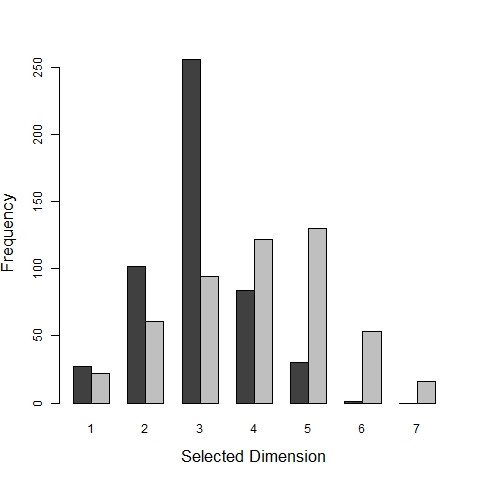
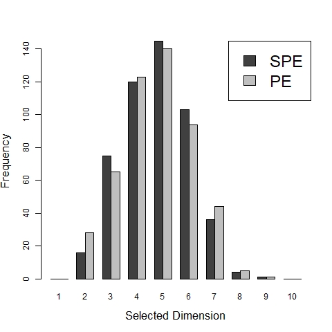
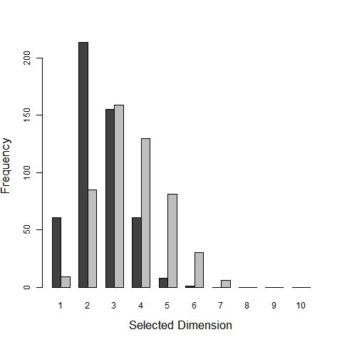
Simulation 2: Data is simulated according to the same parameters as Simulation 1, but u𝑢u is estimated via BIC. Table 2 gives average errors 𝜷^𝜷2superscriptnorm^𝜷𝜷2\|\hat{\bm{\beta}}-\bm{\beta}\|^{2} and Figure 4 in Appendix 8.4 gives histograms of selected envelope dimension u^^𝑢\hat{u}. The SPE improves estimation of 𝜷^^𝜷\hat{\bm{\beta}} over the traditional predictor envelope and the full spatial regression, and improves selection of u^^𝑢\hat{u} over the traditional predictor envelope. It appears that as n𝑛n\rightarrow\infty, the SPE selects to true dimension via BIC with probability approaching one.

Table 2: Average error 𝜷^𝜷2superscriptnorm^𝜷𝜷2\|\hat{\bm{\beta}}-\bm{\beta}\|^{2} with standard deviations in parentheses. Simulation scenario where u<p𝑢𝑝u<p and 𝛀0𝛀1much-less-thannormsubscript𝛀0normsubscript𝛀1\|\bm{\Omega}_{0}\|\ll\|\bm{\Omega}_{1}\|.
n𝑛n SPE PE GLS
50 0.221 (0.015) 0.625 (0.030) 0.530 (0.017)
100 0.075 (0.004) 0.443 (0.020) 0.206 (0.006)
200 0.029 (0.002) 0.370 (0.014) 0.093 (0.002)

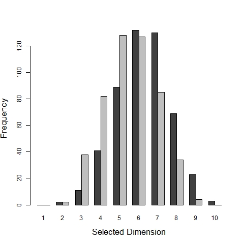
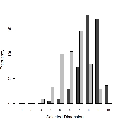
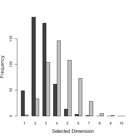
Simulation 3: Data is simulated according to the same parameters as Simulations 1 and 2, but u=p=10𝑢𝑝10u=p=10, 𝛀1=diag{exp(12/3),exp(22/3),,exp(102/3}\bm{\Omega}_{1}=\text{diag}\{\exp(-1^{2/3}),\exp(-2^{2/3}),\ldots,\exp(-10^{2/3}\} and 𝜼=[11]T𝜼superscriptdelimited-[]11𝑇\bm{\eta}=[1\cdots 1]^{T}, meaning 𝚺Xsubscript𝚺𝑋\bm{\Sigma}_{X} has small eigenvalues, but there is no proper envelope subspace. Envelope dimension is unknown and estimated via minimum BIC, giving the SPE an opportunity to falsely estimate a reducing subspace. Table 3 gives average errors 𝜷^𝜷2superscriptnorm^𝜷𝜷2\|\hat{\bm{\beta}}-\bm{\beta}\|^{2} and Figure 5 in Appendix 8.4 gives histograms of selected envelope dimension u^^𝑢\hat{u}. The SPE and GLS estimates perform similarly. The SPE often falsely estimates a reducing subspace via minimum BIC, but apparently not to the detriment (on average) of the regression estimates 𝜷^^𝜷\hat{\bm{\beta}}.

Table 3: Average error 𝜷^𝜷2superscriptnorm^𝜷𝜷2\|\hat{\bm{\beta}}-\bm{\beta}\|^{2} with standard deviations in parentheses. Simulation scenario where u=p𝑢𝑝u=p.
n𝑛n SPE PE GLS
50 0.517 (0.018) 0.970 (0.031) 0.530 (0.017)
100 0.213 (0.007) 0.629 (0.021) 0.206 (0.006)
200 0.091 (0.003) 0.475 (0.015) 0.093 (0.002)

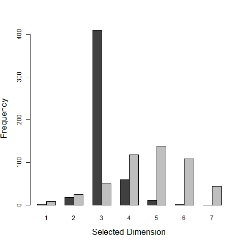
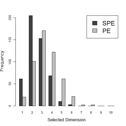
Simulation 4: Data is simulated according to the same parameters as Simulations 1 and 2, but 𝛀1=diag{ω1,ω2,ω3}subscript𝛀1diagsubscript𝜔1subscript𝜔2subscript𝜔3\bm{\Omega}_{1}=\text{diag}\{\omega_{1},\omega_{2},\omega_{3}\} and 𝛀0=diag{ω4,,ω10}subscript𝛀0diagsubscript𝜔4subscript𝜔10\bm{\Omega}_{0}=\text{diag}\{\omega_{4},\ldots,\omega_{10}\}, where ωj,j=1,,10formulae-sequencesubscript𝜔𝑗𝑗110\omega_{j},\ j=1,\dots,10 are randomly generated according to a uniform distribution of [0,1]01[0,1] every iteration. In this way, the magnitudes of 𝛀1normsubscript𝛀1\|\bm{\Omega}_{1}\| and 𝛀0normsubscript𝛀0\|\bm{\Omega}_{0}\| are on average comparable. Table 4 gives average errors 𝜷^𝜷2superscriptnorm^𝜷𝜷2\|\hat{\bm{\beta}}-\bm{\beta}\|^{2} and Figure 6 in Appendix 8.4 gives histograms of selected envelope dimension u^^𝑢\hat{u}. The SPE provides no significant advantage over the GLS estimates in this scenario, due to the comparable magnitudes of 𝛀1\bm{\Omega}_{1}\| and 𝛀1normsubscript𝛀1\|\bm{\Omega}_{1}\|.

Table 4: Average error 𝜷^𝜷2superscriptnorm^𝜷𝜷2\|\hat{\bm{\beta}}-\bm{\beta}\|^{2} with standard deviations in parentheses. Simulation scenario where u<p𝑢𝑝u<p and 𝛀1𝛀0normsubscript𝛀1normsubscript𝛀0\|\bm{\Omega}_{1}\|\approx\|\bm{\Omega}_{0}\|.
n𝑛n SPE PE GLS
50 0.105 (0.015) 0.189 (0.025) 0.122 (0.016)
100 0.040 (0.004) 0.115 (0.013) 0.042 (0.003)
200 0.019 (0.003) 0.151 (0.037) 0.020 (0.002)

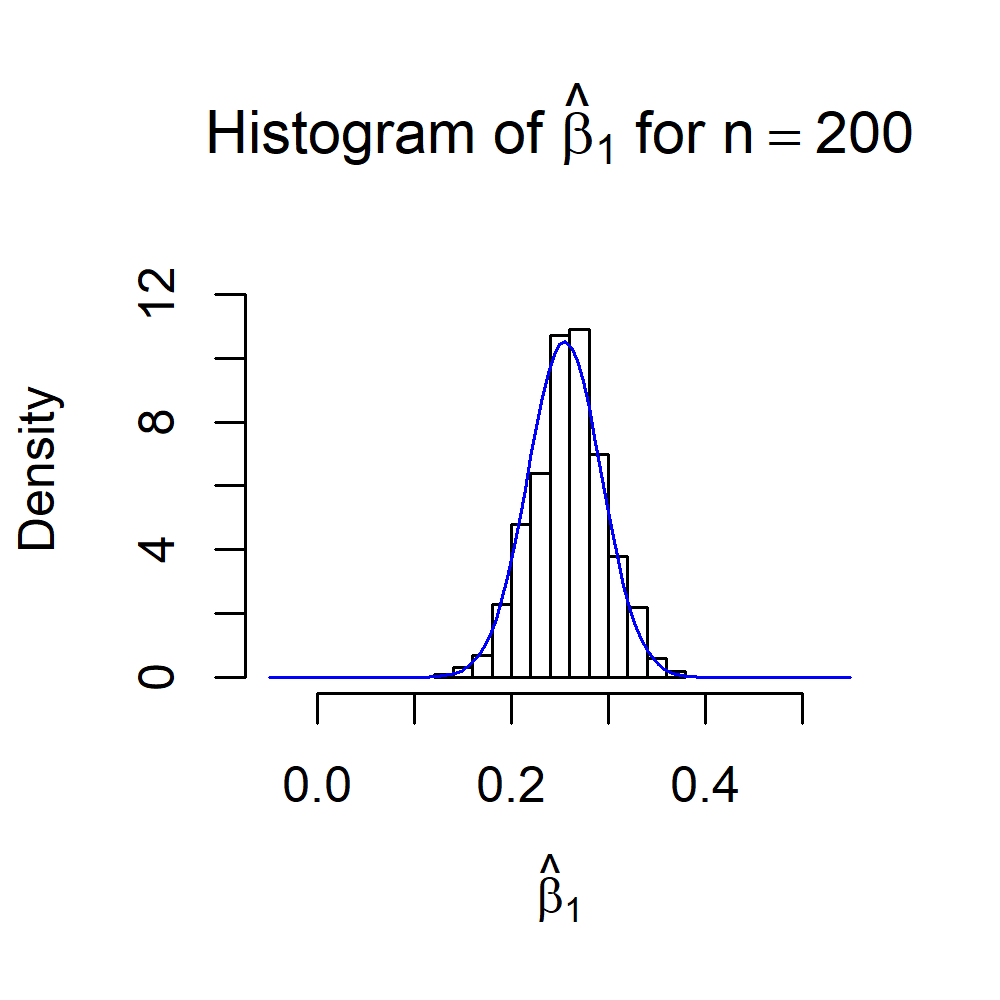
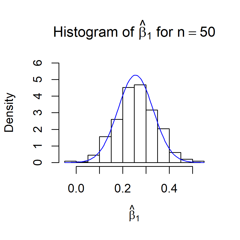
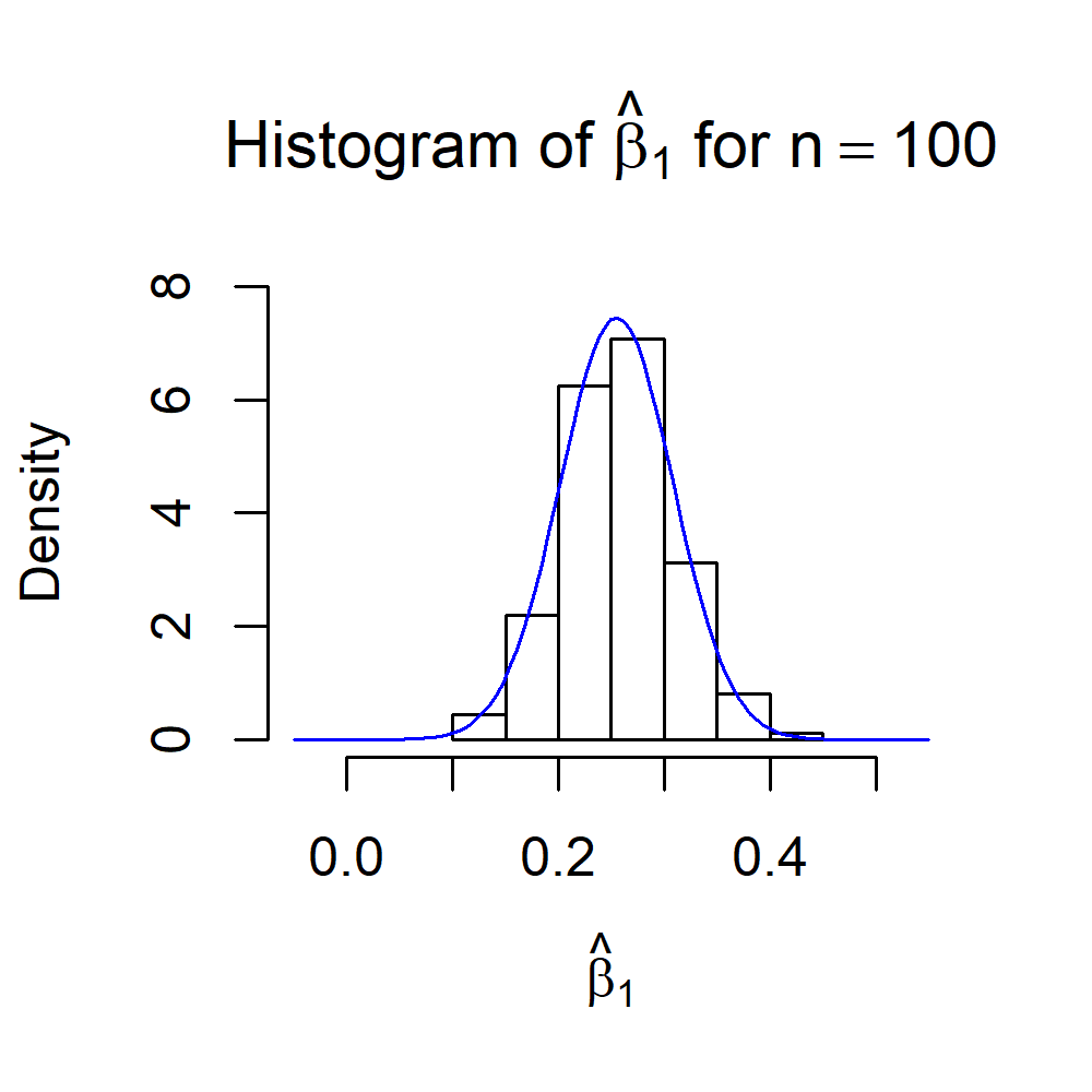
Simulation 5: The asymptotic distributions for 𝜷^^𝜷\hat{\bm{\beta}} given by Equation 24 are compared to the empirical distribution of simulation estimates of 𝜷𝜷\bm{\beta} where θ𝜃\theta is estimated from the data for every sample. The model parameters are the same as Simulations 1 and 2, except that the basis 𝚪1subscript𝚪1\bm{\Gamma}_{1} and the spatial coordinates are randomly generated once and held fixed throughout all 500 simulation iterations. In this way, the variance of 𝜷^^𝜷\hat{\bm{\beta}} for a fixed model can be studied. For the same reason, u𝑢u is considered known and fixed. The simulation is repeated for n=50,100,200𝑛50100200n=50,100,200. Figure 1 gives histograms for the first estimated regression coefficient 𝜷^1subscript^𝜷1\hat{\bm{\beta}}_{1} with the asymptotic normal density given by Equation 24 plotted over-top. The empirical distributions and asymptotic distributions agree well, suggesting that the asymptotic distributions are useful in practice.
Refer to caption
Refer to caption
Refer to caption
Figure 1: Histograms for the first estimated regression coefficient 𝜷^1subscript^𝜷1\hat{\bm{\beta}}_{1} across 500 simulation iterations with the asymptotic normal density given by Equation 24 plotted over-top.

6 Data Analysis

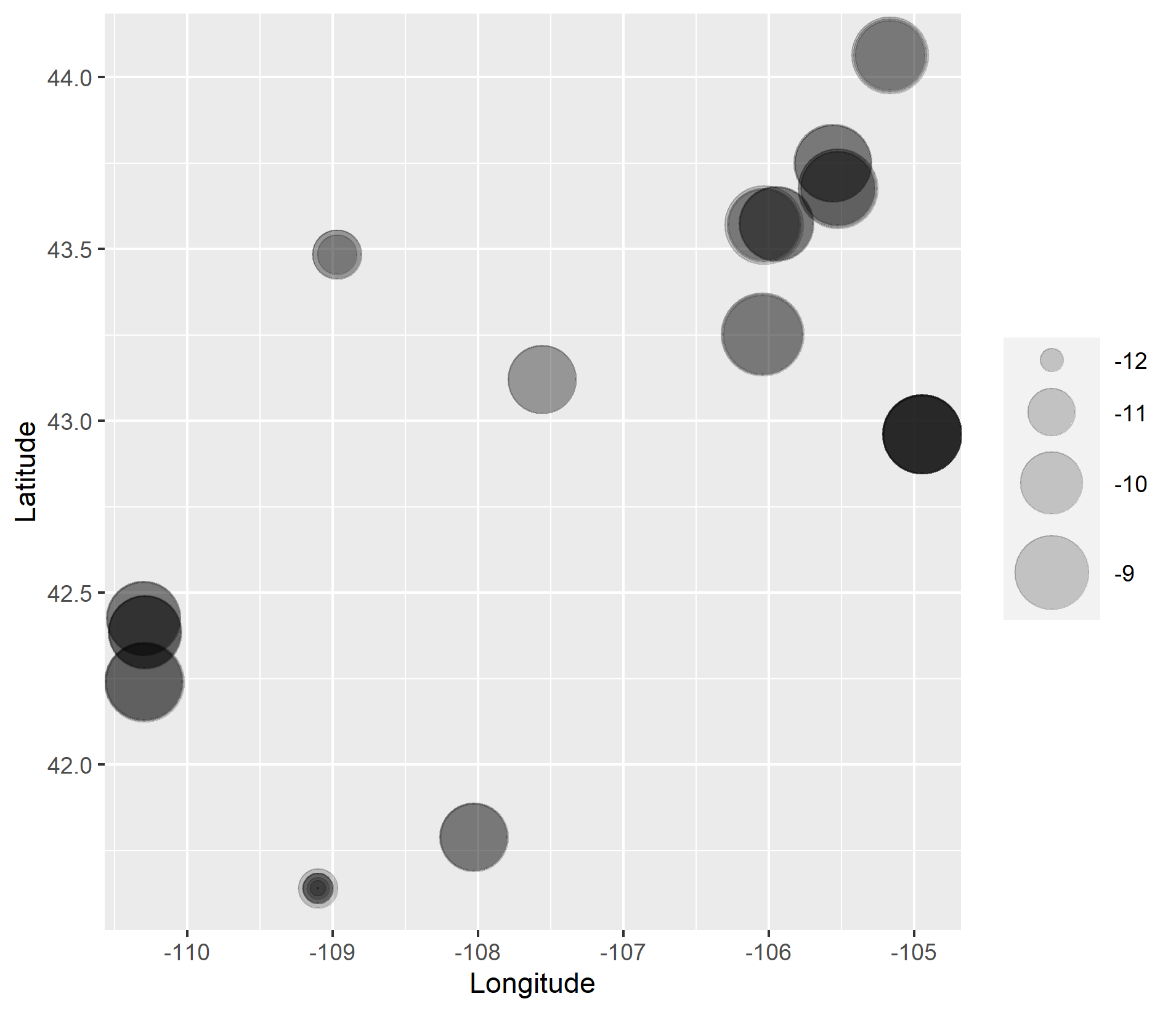
We analyze a geochemical data set to illustrate the spatial predictor envelope. The data set contains 53 samples of the concentrations of 11 major chemical elements and 17 rare earth elements (REEs) at 14 different locations across an oil and gas reserve in Wyoming (Quillinan et al., 2016). The data was collected to assess how rock type / major chemical element concentrations affected the concentration of REEs. REEs are critical to many modern technologies and industrial applications, but economically viable concentrations of REEs are uncommon and tend to occur in uncommon rock types (Van Gosen et al., 2019). There is interest in identifying general mineral characteristics that are correlated with high REE concentrations and using these correlations to identify REE mining prospects; see for example Lands (2014). We follow the techniques of Aitchison (1982) for compositional data, analyzing the log-ratios of the components. The log-concentrations of the 17 REEs are highly positively correlated, with over 95% of the variation explained by the first principal component. With few exceptions, REEs do not occur individually but vary in unison (Hoshino et al., 2016). Therefore, we used the total log-concentration of REEs as the univariate regression response, as it simplifies the model and remains in line with the data analysis goals. We used the log-concentrations of the major chemical elements as a multivariate regression predictor and the SPE to estimate a reducing subspace and linear relationship between the total REE log-concentration and major chemical element log-concentrations. Appendix 8.5 contains more details and justifications on the choice of variables and data transformations. Figure 2 gives the locations and levels of sampled total REE log-concentrations.
Refer to caption
Figure 2: Locations and levels of sampled total REE log-concentrations.

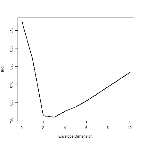
An exponential correlation function with white noise (Equation 25) was used for all correlation functions. The SPE was fit to the data for u=0,,p𝑢0𝑝u=0,\ldots,p and the BIC scores were compared. Figure 3 gives a plot of BIC scores against dimension u𝑢u.

Refer to caption
Figure 3: BIC scores for the SPE for u=0,,p𝑢0𝑝u=0,\ldots,p. The SPE achieves a minimum of 792792792 at u=3𝑢3u=3.

The SPE achieves a minimum BIC of 792792792 at u=3𝑢3u=3. The BIC for the full spatial regression model is 817817817. For reference, the traditional predictor envelope of Cook et al. (2013), designed for independent observations, achieves a minimum BIC of 119711971197, also at u=3𝑢3u=3. The substantially higher BIC score of the traditional predictor envelope when compared to the spatial models suggests accounting for the spatial correlation in this data is crucial. Table 5 gives the estimated coefficients, asymptotic standard errors and Z-scores 𝜷^i/avar[𝜷^i]subscript^𝜷𝑖avardelimited-[]subscript^𝜷𝑖\hat{\bm{\beta}}_{i}/\sqrt{\text{avar}[\hat{\bm{\beta}}_{i}]} for the SPE model with u=3𝑢3u=3. Significant relationships are indicated between several major chemical concentrations and the total REE log-concentration, for example, a positive relationship for potassium oxide (K2O) and phosphorus pentoxide (P2O5) and a negative relationship for magnesium oxide (MgO) and silicon dioxide (SiO2). Alkaline igneous rocks are enriched in potassium and known to be hosts of REE deposits, providing an explanation for the strong positive relationship between potassium oxide and total REE log-concentration (Dostal, 2017).

Table 5: Estimated coefficients, asymptotic standard errors and Z-scores 𝜷^i/avar[𝜷^i]subscript^𝜷𝑖avardelimited-[]subscript^𝜷𝑖\hat{\bm{\beta}}_{i}/\sqrt{\text{avar}[\hat{\bm{\beta}}_{i}]} for each of the major chemical components.
Chemical CaO Fe2O3 K2O LOI MgO MnO Na2O P2O5 SiO2 TiO2
𝜷^isubscript^𝜷𝑖\hat{\bm{\beta}}_{i} -0.10 -0.12 0.36 -0.05 -0.21 0.03 0.02 0.22 -0.29 0.10
avar[𝜷^i]avardelimited-[]subscript^𝜷𝑖\sqrt{\text{avar}[\hat{\bm{\beta}}_{i}]} 0.08 0.09 0.08 0.09 0.07 0.07 0.06 0.09 0.10 0.10
Z-score -1.28 -1.35 4.50 -0.58 -3.13 0.38 0.45 2.57 -2.73 1.03

To compare the predictive performance of the SPE against traditional spatial regression (GLS), a cross-validation study was performed on the data. A hundred iterations of 10-fold cross-validation was performed, with predictions of the test data performed using the conditional expectation

Y^test=E[Ytest|Ytrain,𝜷^,θ^]=Xtest𝜷^+E[ϵtest|ϵtrain,θ^]subscript^𝑌test𝐸delimited-[]conditionalsubscript𝑌testsubscript𝑌train^𝜷^𝜃subscript𝑋test^𝜷𝐸delimited-[]conditionalsubscriptitalic-ϵtestsubscriptitalic-ϵtrain^𝜃\hat{Y}_{\text{test}}=E[Y_{\text{test}}|Y_{\text{train}},\hat{\bm{\beta}},\hat{\theta}]=X_{\text{test}}\hat{\bm{\beta}}+E[\epsilon_{\text{test}}|\epsilon_{\text{train}},\hat{\theta}]

where the conditional expectation of the error terms is given by the kriging equation (Matheron, 1982; Cressie, 2015). The predictions were compared by their mean squared prediction error (MSPE), calculated as

MSPE=1Ni=1N(Y^test,iYtest,i)2,MSPE1𝑁superscriptsubscript𝑖1𝑁superscriptsubscript^𝑌test𝑖subscript𝑌test𝑖2\text{MSPE}=\frac{1}{N}\sum_{i=1}^{N}(\hat{Y}_{\text{test},i}-Y_{\text{test},i})^{2},

where N𝑁N is the number of predicted observations. The average MSPE for the SPE and spatial regression was 0.09 and 0.16 respectively, showing significant improvement in prediction through the dimension reduction of the predictors. For context, the sample variance of the response, 1ni=1n(YiY¯)21𝑛superscriptsubscript𝑖1𝑛superscriptsubscript𝑌𝑖¯𝑌2\frac{1}{n}\sum_{i=1}^{n}(Y_{i}-\bar{Y})^{2}, is 1.31, meaning both methods predicted a substantial portion of the variation in the response.

7 Discussion

The proposed spatial predictor envelope provides an effective tool for multivariate spatial data. By reducing the dimension of the predictors through a likelihood-based approach, the SPE can improve estimation of the regression coefficients and prediction of the response over traditional spatial regression. The SPE improves estimation/prediction over the original predictor envelope for spatial data by accounting for spatial correlation.

In this paper, the asymptotic distribution for the estimable parameters is given for known spatial correlation parameters θ𝜃\theta. The difficulty in deriving asymptotic distributions for unknown θ𝜃\theta are two-fold. First, to apply the results of Shapiro (1986), a discrepancy function satisfying certain regularity conditions must be devised such that the parameters that minimize the discrepancy function are equivalent to the parameters that maximize the likelihood. Second, the results of Shapiro (1986) hinge upon the parameter estimates of the full, unconstrained model being consistent and asymptotically normal. This is a difficult problem in spatial statistics, where the answer often depends on the sampling scheme of the locations s1,,snsubscript𝑠1subscript𝑠𝑛s_{1},\ldots,s_{n} and the spatial correlation function (Mardia and Marshall, 1984; Zhang, 2004).

The assumption of normality may be too restrictive for some applications. Cook and Zhang (2015) discuss envelope models in a generalized linear model context. Generalized linear mixed models are popular for modeling non-Gaussian spatial data, see for example Zhang (2002). Expanding spatial envelopes to the general linear mixed model setting would be a worthy task.

References

  • Aitchison (1982) John Aitchison. The statistical analysis of compositional data. Journal of the Royal Statistical Society: Series B (Methodological), 44(2):139–160, 1982.
  • Beguería et al. (2013) Santiago Beguería, Valentina Spanu, Ana Navas, Javier Machín, and Marta Angulo-Martínez. Modeling the spatial distribution of soil properties by generalized least squares regression: Toward a general theory of spatial variates. Journal of soil and water conservation, 68(3):172–184, 2013.
  • Björck and Golub (1973) Ake Björck and Gene H Golub. Numerical methods for computing angles between linear subspaces. Mathematics of computation, 27(123):579–594, 1973.
  • Borchers (2019) Hans W. Borchers. pracma: Practical Numerical Math Functions, 2019. URL https://CRAN.R-project.org/package=pracma. R package version 2.2.5.
  • Cook (2018) R Dennis Cook. An introduction to envelopes: dimension reduction for efficient estimation in multivariate statistics, volume 401. John Wiley & Sons, 2018.
  • Cook and Zhang (2015) R Dennis Cook and Xin Zhang. Foundations for envelope models and methods. Journal of the American Statistical Association, 110(510):599–611, 2015.
  • Cook et al. (2010) R Dennis Cook, Bing Li, and Francesca Chiaromonte. Envelope models for parsimonious and efficient multivariate linear regression. Statistica Sinica, pages 927–960, 2010.
  • Cook et al. (2016) R Dennis Cook, Liliana Forzani, and Zhihua Su. A note on fast envelope estimation. Journal of Multivariate Analysis, 150:42–54, 2016.
  • Cook et al. (2013) RD Cook, IS Helland, and Z Su. Envelopes and partial least squares regression. Journal of the Royal Statistical Society: Series B (Statistical Methodology), 75(5):851–877, 2013.
  • Cressie (2015) Noel Cressie. Statistics for spatial data. John Wiley & Sons, 2015.
  • Dostal (2017) Jaroslav Dostal. Rare Earth Element Deposits of Alkaline Igneous Rocks. Resources, 6:34, 07 2017. doi: 10.3390/resources6030034.
  • Genton (2001) Marc G Genton. Classes of kernels for machine learning: a statistics perspective. Journal of machine learning research, 2(Dec):299–312, 2001.
  • Hengl et al. (2007) Tomislav Hengl, Gerard BM Heuvelink, and David G Rossiter. About regression-kriging: From equations to case studies. Computers & geosciences, 33(10):1301–1315, 2007.
  • Hoff and Franks (2019) Peter Hoff and Alexander Franks. rstiefel: Random Orthonormal Matrix Generation and Optimization on the Stiefel Manifold, 2019. URL https://CRAN.R-project.org/package=rstiefel. R package version 1.0.0.
  • Hoshino et al. (2016) M. Hoshino, K. Sanematsu, and Y. Watanabe. Chapter 279 - REE Mineralogy and Resources. In Bünzli Jean-Claude and Pecharsky Vitalij K., editors, Including Actinides, volume 49 of Handbook on the Physics and Chemistry of Rare Earths, pages 129–291. Elsevier, 2016. doi: https://doi.org/10.1016/bs.hpcre.2016.03.006. URL https://www.sciencedirect.com/science/article/pii/S0168127316300010.
  • Junttila and Laine (2017) Virpi Junttila and Marko Laine. Bayesian principal component regression model with spatial effects for forest inventory variables under small field sample size. Remote Sensing of Environment, 192:45–57, 2017.
  • Lambert et al. (2004) Dayton M Lambert, James Lowenberg-Deboer, and Rodolfo Bongiovanni. A comparison of four spatial regression models for yield monitor data: A case study from argentina. Precision Agriculture, 5(6):579–600, 2004.
  • Lands (2014) Utah Trust Lands. Rare earth element prospects and occurrences in Utah. Technical report, Utah Geological Survey, 01 2014.
  • Lee and Su (2020) Minji Lee and Zhihua Su. A review of envelope models. International Statistical Review, 88(3):658–676, 2020.
  • Mardia and Goodall (1993) Kanti V Mardia and Colin R Goodall. Spatial-temporal analysis of multivariate environmental monitoring data. Multivariate environmental statistics, 6(76):347–385, 1993.
  • Mardia and Marshall (1984) Kanti V Mardia and Roger J Marshall. Maximum likelihood estimation of models for residual covariance in spatial regression. Biometrika, 71(1):135–146, 1984.
  • Matheron (1982) G. Matheron. Pour une Analyse Krigeante des Données Régionalisées. Cent. de Geostat, 1982.
  • Mezzadri (2006) Francesco Mezzadri. How to generate random matrices from the classical compact groups. arXiv preprint math-ph/0609050, 2006.
  • Quillinan et al. (2016) Scott Quillinan, Charles Nye, Travis McLing, and Hari Neupane. Rare Earth Element Geochemistry for Produced Waters, WY. 6 2016. doi: 10.15121/1360765. URL https://www.osti.gov/biblio/1360765.
  • R Core Team (2019) R Core Team. R: A Language and Environment for Statistical Computing. R Foundation for Statistical Computing, Vienna, Austria, 2019. URL https://www.R-project.org/.
  • Rekabdarkolaee et al. (2020) Hossein Moradi Rekabdarkolaee, Qin Wang, Zahra Naji, and Montserrat Fuentes. New parsimonious multivariate spatial model: Spatial envelope. Statistica Sinica, 30(3), 2020.
  • Sampson et al. (2013) Paul D Sampson, Mark Richards, Adam A Szpiro, Silas Bergen, Lianne Sheppard, Timothy V Larson, and Joel D Kaufman. A regionalized national universal kriging model using Partial Least Squares regression for estimating annual PM2. 5 concentrations in epidemiology. Atmospheric environment, 75:383–392, 2013.
  • Shapiro (1986) Alexander Shapiro. Asymptotic theory of overparameterized structural models. Journal of the American Statistical Association, 81(393):142–149, 1986.
  • Stein (2012) Michael L Stein. Interpolation of spatial data: some theory for kriging. Springer Science & Business Media, 2012.
  • Taylor-Rodriguez et al. (2019) Daniel Taylor-Rodriguez, Andrew O Finley, Abhirup Datta, Chad Babcock, Hans-Erik Andersen, Bruce D Cook, Douglas C Morton, and Sudipto Banerjee. Spatial factor models for high-dimensional and large spatial data: An application in forest variable mapping. Statistica Sinica, 29:1155, 2019.
  • Van Gosen et al. (2019) Bradley S Van Gosen, Philip L Verplanck, and Poul Emsbo. Rare earth element mineral deposits in the United States. Technical report, US Geological Survey, 2019.
  • Wen and Yin (2013) Zaiwen Wen and Wotao Yin. A feasible method for optimization with orthogonality constraints. Mathematical Programming, 142(1-2):397–434, 2013.
  • Wijewardane et al. (2016) Nuwan K Wijewardane, Yufeng Ge, Skye Wills, and Terry Loecke. Prediction of soil carbon in the conterminous United States: Visible and near infrared reflectance spectroscopy analysis of the rapid carbon assessment project. Soil Science Society of America Journal, 80(4):973–982, 2016.
  • Zhang (2002) Hao Zhang. On estimation and prediction for spatial generalized linear mixed models. Biometrics, 58(1):129–136, 2002.
  • Zhang (2004) Hao Zhang. Inconsistent estimation and asymptotically equal interpolations in model-based geostatistics. Journal of the American Statistical Association, 99(465):250–261, 2004.

8 Appendix

8.1 Maximum Likelihood Estimation

Let 𝒀𝒀\bm{Y} and 𝑿𝑿\bm{X} be n×r𝑛𝑟n\times r and n×p𝑛𝑝n\times p matrices of observations at locations s1,,snsubscript𝑠1subscript𝑠𝑛s_{1},\ldots,s_{n} and 𝝆(θ)𝝆𝜃\bm{\rho}(\theta) be the n×n𝑛𝑛n\times n correlation matrix where 𝝆(θ)ij=ρθ(si,sj)𝝆subscript𝜃𝑖𝑗subscript𝜌𝜃subscript𝑠𝑖subscript𝑠𝑗\bm{\rho}(\theta)_{ij}=\rho_{\theta}(s_{i},s_{j}). Let 11\vec{1} be a n×1𝑛1n\times 1 vector of ones and 𝒀~=[1𝒀]~𝒀delimited-[]1𝒀\tilde{\bm{Y}}=[\vec{1}\ \bm{Y}], 𝑿~=[1𝑿]~𝑿delimited-[]1𝑿\tilde{\bm{X}}=[\vec{1}\ \bm{X}]. Assume the envelope dimension u𝑢u is known.

Derivation of the estimates is easiest if the joint log-likelihood L(𝑿,𝒀)𝐿𝑿𝒀L(\bm{X},\bm{Y}) is decomposed into L(𝑿,𝒀)=L(𝑿|𝒀)+L(𝒀)𝐿𝑿𝒀𝐿conditional𝑿𝒀𝐿𝒀L(\bm{X},\bm{Y})=L(\bm{X}|\bm{Y})+L(\bm{Y}). First, see that

𝚺X|Ysubscript𝚺conditional𝑋𝑌\displaystyle\bm{\Sigma}_{X|Y} =𝚺X𝚺XY𝚺Y1𝚺XYTabsentsubscript𝚺𝑋subscript𝚺𝑋𝑌superscriptsubscript𝚺𝑌1superscriptsubscript𝚺𝑋𝑌𝑇\displaystyle=\bm{\Sigma}_{X}-\bm{\Sigma}_{XY}\bm{\Sigma}_{Y}^{-1}\bm{\Sigma}_{XY}^{T}
=𝚪1𝛀1𝚪1T+𝚪0𝛀0𝚪0T𝚪1𝛀1𝜼𝚺Y1(𝚪1𝛀1𝜼)Tabsentsubscript𝚪1subscript𝛀1superscriptsubscript𝚪1𝑇subscript𝚪0subscript𝛀0superscriptsubscript𝚪0𝑇subscript𝚪1subscript𝛀1𝜼superscriptsubscript𝚺𝑌1superscriptsubscript𝚪1subscript𝛀1𝜼𝑇\displaystyle=\bm{\Gamma}_{1}\bm{\Omega}_{1}\bm{\Gamma}_{1}^{T}+\bm{\Gamma}_{0}\bm{\Omega}_{0}\bm{\Gamma}_{0}^{T}-\bm{\Gamma}_{1}\bm{\Omega}_{1}\bm{\eta}\bm{\Sigma}_{Y}^{-1}(\bm{\Gamma}_{1}\bm{\Omega}_{1}\bm{\eta})^{T}
=𝚪1(𝛀1(𝛀1𝜼)𝚺Y1(𝛀1𝜼)T)𝚪1T+𝚪0𝛀0𝚪0Tabsentsubscript𝚪1subscript𝛀1subscript𝛀1𝜼superscriptsubscript𝚺𝑌1superscriptsubscript𝛀1𝜼𝑇superscriptsubscript𝚪1𝑇subscript𝚪0subscript𝛀0superscriptsubscript𝚪0𝑇\displaystyle=\bm{\Gamma}_{1}(\bm{\Omega}_{1}-(\bm{\Omega}_{1}\bm{\eta})\bm{\Sigma}_{Y}^{-1}(\bm{\Omega}_{1}\bm{\eta})^{T})\bm{\Gamma}_{1}^{T}+\bm{\Gamma}_{0}\bm{\Omega}_{0}\bm{\Gamma}_{0}^{T}
𝚪1𝛀1𝚪1T+𝚪0𝛀0𝚪0T,absentsubscript𝚪1superscriptsubscript𝛀1superscriptsubscript𝚪1𝑇subscript𝚪0subscript𝛀0superscriptsubscript𝚪0𝑇\displaystyle\equiv\bm{\Gamma}_{1}\bm{\Omega}_{1}^{*}\bm{\Gamma}_{1}^{T}+\bm{\Gamma}_{0}\bm{\Omega}_{0}\bm{\Gamma}_{0}^{T},

showing that 𝚺X|Ysubscript𝚺conditional𝑋𝑌\bm{\Sigma}_{X|Y} has the same decomposition as 𝚺Xsubscript𝚺𝑋\bm{\Sigma}_{X}, but the material variation 𝛀1=𝛀1(𝛀1𝜼)𝚺Y1(𝛀1𝜼)Tsuperscriptsubscript𝛀1subscript𝛀1subscript𝛀1𝜼superscriptsubscript𝚺𝑌1superscriptsubscript𝛀1𝜼𝑇\bm{\Omega}_{1}^{*}=\bm{\Omega}_{1}-(\bm{\Omega}_{1}\bm{\eta})\bm{\Sigma}_{Y}^{-1}(\bm{\Omega}_{1}\bm{\eta})^{T} has been reduced by the variation explained by 𝒀𝒀\bm{Y}. Next, given the regression equation X(s)|Y(s)=μX|Y+𝜷XTY+ϵX|Y(s)conditional𝑋𝑠𝑌𝑠subscript𝜇conditional𝑋𝑌superscriptsubscript𝜷𝑋𝑇𝑌subscriptitalic-ϵconditional𝑋𝑌𝑠\vec{X}(s)|\vec{Y}(s)=\vec{\mu}_{X|Y}+\bm{\beta}_{X}^{T}\vec{Y}+\vec{\epsilon}_{X|Y}(s) the reverse regression coefficients 𝜷Xsubscript𝜷𝑋\bm{\beta}_{X} can be written as

𝜷Xsubscript𝜷𝑋\displaystyle\bm{\beta}_{X} =𝚺Y1𝚺XYTabsentsuperscriptsubscript𝚺𝑌1superscriptsubscript𝚺𝑋𝑌𝑇\displaystyle=\bm{\Sigma}_{Y}^{-1}\bm{\Sigma}_{XY}^{T}
=𝚺Y1(𝚪1𝛀1𝜼)Tabsentsuperscriptsubscript𝚺𝑌1superscriptsubscript𝚪1subscript𝛀1𝜼𝑇\displaystyle=\bm{\Sigma}_{Y}^{-1}(\bm{\Gamma}_{1}\bm{\Omega}_{1}\bm{\eta})^{T}
(𝚪1𝜼X)T,absentsuperscriptsubscript𝚪1subscript𝜼𝑋𝑇\displaystyle\equiv(\bm{\Gamma}_{1}\bm{\eta}_{X})^{T},

where 𝜼X=𝛀1𝜼𝚺Y1subscript𝜼𝑋subscript𝛀1𝜼superscriptsubscript𝚺𝑌1\bm{\eta}_{X}=\bm{\Omega}_{1}\bm{\eta}\bm{\Sigma}_{Y}^{-1}, showing that 𝜷Xsubscript𝜷𝑋\bm{\beta}_{X} has the same form as 𝜷𝜷\bm{\beta}.

Using properties of the Kronecker product, |𝚺X|Y𝝆(θ)|=|𝚺X|Y|n|𝝆(θ)|ptensor-productsubscript𝚺conditional𝑋𝑌𝝆𝜃superscriptsubscript𝚺conditional𝑋𝑌𝑛superscript𝝆𝜃𝑝|\bm{\Sigma}_{X|Y}\otimes\bm{\rho}(\theta)|=|\bm{\Sigma}_{X|Y}|^{n}|\bm{\rho}(\theta)|^{p}. Finally, because 𝚪1,𝚪0subscript𝚪1subscript𝚪0\bm{\Gamma}_{1},\ \bm{\Gamma}_{0} are orthogonal, |𝚺X|Y|=|𝛀1||𝛀0|subscript𝚺conditional𝑋𝑌superscriptsubscript𝛀1subscript𝛀0|\bm{\Sigma}_{X|Y}|=|\bm{\Omega}_{1}^{*}||\bm{\Omega}_{0}|.

Now prepared to embark, the log-likelihood can be written as

L(𝑿,𝒀)=𝐿𝑿𝒀absent\displaystyle L(\bm{X},\bm{Y})= n2|𝚺X|Y|12vec(𝑿1μX|YT𝒀𝜷X)T(𝚺X|Y𝝆(θ))1vec(𝑿1μX|YT𝒀𝜷X)𝑛2subscript𝚺conditional𝑋𝑌12vecsuperscript𝑿1superscriptsubscript𝜇conditional𝑋𝑌𝑇𝒀subscript𝜷𝑋𝑇superscripttensor-productsubscript𝚺conditional𝑋𝑌𝝆𝜃1vec𝑿1superscriptsubscript𝜇conditional𝑋𝑌𝑇𝒀subscript𝜷𝑋\displaystyle-\frac{n}{2}|\bm{\Sigma}_{X|Y}|-\frac{1}{2}\mathrm{vec}(\bm{X}-\vec{1}\vec{\mu}_{X|Y}^{T}-\bm{Y}\bm{\beta}_{X})^{T}(\bm{\Sigma}_{X|Y}\otimes\bm{\rho}(\theta))^{-1}\mathrm{vec}(\bm{X}-\vec{1}\vec{\mu}_{X|Y}^{T}-\bm{Y}\bm{\beta}_{X})
n(p+r)2log(2π)p+r2|𝝆(θ)|𝑛𝑝𝑟22𝜋𝑝𝑟2𝝆𝜃\displaystyle-\frac{n(p+r)}{2}\log(2\pi)-\frac{p+r}{2}|\bm{\rho}(\theta)|
n2|𝚺Y|12vec(𝒀1μYT)T(𝚺Y𝝆(θ))1vec(𝒀1μYT)𝑛2subscript𝚺𝑌12vecsuperscript𝒀1superscriptsubscript𝜇𝑌𝑇𝑇superscripttensor-productsubscript𝚺𝑌𝝆𝜃1vec𝒀1superscriptsubscript𝜇𝑌𝑇\displaystyle-\frac{n}{2}|\bm{\Sigma}_{Y}|-\frac{1}{2}\mathrm{vec}(\bm{Y}-\vec{1}\vec{\mu}_{Y}^{T})^{T}(\bm{\Sigma}_{Y}\otimes\bm{\rho}(\theta))^{-1}\mathrm{vec}(\bm{Y}-\vec{1}\vec{\mu}_{Y}^{T})
=\displaystyle= n2|𝛀1|12vec(𝑿𝚪11μX|YT𝚪1𝒀𝜼XT)(𝛀1𝝆(θ))1vec(𝑿𝚪11μX|YT𝚪1𝒀𝜼XT)𝑛2superscriptsubscript𝛀112vec𝑿subscript𝚪11superscriptsubscript𝜇conditional𝑋𝑌𝑇subscript𝚪1𝒀superscriptsubscript𝜼𝑋𝑇superscripttensor-productsuperscriptsubscript𝛀1𝝆𝜃1vec𝑿subscript𝚪11superscriptsubscript𝜇conditional𝑋𝑌𝑇subscript𝚪1𝒀superscriptsubscript𝜼𝑋𝑇\displaystyle-\frac{n}{2}|\bm{\Omega}_{1}^{*}|-\frac{1}{2}\mathrm{vec}(\bm{X}\bm{\Gamma}_{1}-\vec{1}\vec{\mu}_{X|Y}^{T}\bm{\Gamma}_{1}-\bm{Y}\bm{\eta}_{X}^{T})(\bm{\Omega}_{1}^{*}\otimes\bm{\rho}(\theta))^{-1}\mathrm{vec}(\bm{X}\bm{\Gamma}_{1}-\vec{1}\vec{\mu}_{X|Y}^{T}\bm{\Gamma}_{1}-\bm{Y}\bm{\eta}_{X}^{T})
n2|𝛀0|12vec(𝑿𝚪01μX|YT𝚪0)(𝛀0𝝆(θ))1vec(𝑿𝚪01μX|YT𝚪0)𝑛2subscript𝛀012vec𝑿subscript𝚪01superscriptsubscript𝜇conditional𝑋𝑌𝑇subscript𝚪0superscripttensor-productsubscript𝛀0𝝆𝜃1vec𝑿subscript𝚪01superscriptsubscript𝜇conditional𝑋𝑌𝑇subscript𝚪0\displaystyle-\frac{n}{2}|\bm{\Omega}_{0}|-\frac{1}{2}\mathrm{vec}(\bm{X}\bm{\Gamma}_{0}-\vec{1}\vec{\mu}_{X|Y}^{T}\bm{\Gamma}_{0})(\bm{\Omega}_{0}\otimes\bm{\rho}(\theta))^{-1}\mathrm{vec}(\bm{X}\bm{\Gamma}_{0}-\vec{1}\vec{\mu}_{X|Y}^{T}\bm{\Gamma}_{0})
n(p+r)2log(2π)p+r2|𝝆(θ)|𝑛𝑝𝑟22𝜋𝑝𝑟2𝝆𝜃\displaystyle-\frac{n(p+r)}{2}\log(2\pi)-\frac{p+r}{2}|\bm{\rho}(\theta)|
n2|𝚺Y|12vec(𝒀1μYT)T(𝚺Y𝝆(θ))1vec(𝒀1μYT).𝑛2subscript𝚺𝑌12vecsuperscript𝒀1superscriptsubscript𝜇𝑌𝑇𝑇superscripttensor-productsubscript𝚺𝑌𝝆𝜃1vec𝒀1superscriptsubscript𝜇𝑌𝑇\displaystyle-\frac{n}{2}|\bm{\Sigma}_{Y}|-\frac{1}{2}\mathrm{vec}(\bm{Y}-\vec{1}\vec{\mu}_{Y}^{T})^{T}(\bm{\Sigma}_{Y}\otimes\bm{\rho}(\theta))^{-1}\mathrm{vec}(\bm{Y}-\vec{1}\vec{\mu}_{Y}^{T}).

Let μ1=𝚪1μX|Ysubscript𝜇1subscript𝚪1subscript𝜇conditional𝑋𝑌\vec{\mu}_{1}=\bm{\Gamma}_{1}\vec{\mu}_{X|Y} and μ0=𝚪0μX|Ysubscript𝜇0subscript𝚪0subscript𝜇conditional𝑋𝑌\vec{\mu}_{0}=\bm{\Gamma}_{0}\vec{\mu}_{X|Y}. Taking derivatives and equating to zero shows maximums are achieved at

B^1[μ^1𝜼^X]subscript^B1matrixsubscript^𝜇1subscript^𝜼𝑋\displaystyle\hat{\textbf{B}}_{1}\equiv\begin{bmatrix}\hat{\mu}_{1}\\ \hat{\bm{\eta}}_{X}\end{bmatrix} =((𝒀~T𝝆(θ)1𝒀~)1𝒀~T𝝆(θ)1𝑿𝚪1)Tabsentsuperscriptsuperscriptsuperscript~𝒀𝑇𝝆superscript𝜃1~𝒀1superscript~𝒀𝑇𝝆superscript𝜃1𝑿subscript𝚪1𝑇\displaystyle=\left((\tilde{\bm{Y}}^{T}\bm{\rho}(\theta)^{-1}\tilde{\bm{Y}})^{-1}\tilde{\bm{Y}}^{T}\bm{\rho}(\theta)^{-1}\bm{X}\bm{\Gamma}_{1}\right)^{T}
μ^0subscript^𝜇0\displaystyle\hat{\mu}_{0} =((1T𝝆(θ)11)11T𝝆(θ)1𝑿𝚪1)Tabsentsuperscriptsuperscriptsuperscript1𝑇𝝆superscript𝜃111superscript1𝑇𝝆superscript𝜃1𝑿subscript𝚪1𝑇\displaystyle=\left((\vec{1}^{T}\bm{\rho}(\theta)^{-1}\vec{1})^{-1}\vec{1}^{T}\bm{\rho}(\theta)^{-1}\bm{X}\bm{\Gamma}_{1}\right)^{T}
μ^Ysubscript^𝜇𝑌\displaystyle\hat{\mu}_{Y} =((1T𝝆(θ)11)11T𝝆(θ)1𝒀)Tabsentsuperscriptsuperscriptsuperscript1𝑇𝝆superscript𝜃111superscript1𝑇𝝆superscript𝜃1𝒀𝑇\displaystyle=\left((\vec{1}^{T}\bm{\rho}(\theta)^{-1}\vec{1})^{-1}\vec{1}^{T}\bm{\rho}(\theta)^{-1}\bm{Y}\right)^{T}
𝛀^1superscriptsubscript^𝛀1\displaystyle\hat{\bm{\Omega}}_{1}^{*} =(𝑿𝚪1𝒀~B^1T)T𝝆(θ)1(𝑿𝚪1𝒀~B^1T)absentsuperscript𝑿subscript𝚪1~𝒀superscriptsubscript^B1𝑇𝑇𝝆superscript𝜃1𝑿subscript𝚪1~𝒀superscriptsubscript^B1𝑇\displaystyle=(\bm{X}\bm{\Gamma}_{1}-\tilde{\bm{Y}}\hat{\textbf{B}}_{1}^{T})^{T}\bm{\rho}(\theta)^{-1}(\bm{X}\bm{\Gamma}_{1}-\tilde{\bm{Y}}\hat{\textbf{B}}_{1}^{T})
=𝚪1T𝑺X|Y(θ)𝚪1absentsuperscriptsubscript𝚪1𝑇subscript𝑺conditional𝑋𝑌𝜃subscript𝚪1\displaystyle=\bm{\Gamma}_{1}^{T}\bm{S}_{X|Y}(\theta)\bm{\Gamma}_{1}
𝛀^0subscript^𝛀0\displaystyle\hat{\bm{\Omega}}_{0} =(𝑿𝚪01μ^0T)T𝝆(θ)1(𝑿𝚪01μ^0T)absentsuperscript𝑿subscript𝚪01superscriptsubscript^𝜇0𝑇𝑇𝝆superscript𝜃1𝑿subscript𝚪01superscriptsubscript^𝜇0𝑇\displaystyle=(\bm{X}\bm{\Gamma}_{0}-\vec{1}\hat{\mu}_{0}^{T})^{T}\bm{\rho}(\theta)^{-1}(\bm{X}\bm{\Gamma}_{0}-\vec{1}\hat{\mu}_{0}^{T})
=𝚪0T𝑺X(θ)𝚪0absentsuperscriptsubscript𝚪0𝑇subscript𝑺𝑋𝜃subscript𝚪0\displaystyle=\bm{\Gamma}_{0}^{T}\bm{S}_{X}(\theta)\bm{\Gamma}_{0}
𝚺^Ysubscript^𝚺𝑌\displaystyle\hat{\bm{\Sigma}}_{Y} =(𝒀1μ^YT)T𝝆(θ)1(𝒀1μ^YT)absentsuperscript𝒀1superscriptsubscript^𝜇𝑌𝑇𝑇𝝆superscript𝜃1𝒀1superscriptsubscript^𝜇𝑌𝑇\displaystyle=(\bm{Y}-\vec{1}\hat{\mu}_{Y}^{T})^{T}\bm{\rho}(\theta)^{-1}(\bm{Y}-\vec{1}\hat{\mu}_{Y}^{T})
=𝑺Y(θ),absentsubscript𝑺𝑌𝜃\displaystyle=\bm{S}_{Y}(\theta),

where 𝑺X|Y(θ)subscript𝑺conditional𝑋𝑌𝜃\bm{S}_{X|Y}(\theta), 𝑺X(θ)subscript𝑺𝑋𝜃\bm{S}_{X}(\theta) and 𝑺Y(θ)subscript𝑺𝑌𝜃\bm{S}_{Y}(\theta) are the sample covariance matrices defined in Equations 16. Substituting these quantities into the log-likelihood gives the partially maximized log-likelihood

L1(𝑿,𝒀)=subscript𝐿1𝑿𝒀absent\displaystyle L_{1}(\bm{X},\bm{Y})= n2log|𝚪1T𝑺X|Y(θ)𝚪1|n2log|𝚪0T𝑺X(θ)𝚪0|n2log|𝑺Y(θ)|p+r2log|𝝆(θ)|𝑛2superscriptsubscript𝚪1𝑇subscript𝑺conditional𝑋𝑌𝜃subscript𝚪1𝑛2superscriptsubscript𝚪0𝑇subscript𝑺𝑋𝜃subscript𝚪0𝑛2subscript𝑺𝑌𝜃𝑝𝑟2𝝆𝜃\displaystyle-\frac{n}{2}\log|\bm{\Gamma}_{1}^{T}\bm{S}_{X|Y}(\theta)\bm{\Gamma}_{1}|-\frac{n}{2}\log|\bm{\Gamma}_{0}^{T}\bm{S}_{X}(\theta)\bm{\Gamma}_{0}|-\frac{n}{2}\log|\bm{S}_{Y}(\theta)|-\frac{p+r}{2}\log|\bm{\rho}(\theta)|
n(p+r)2log(2π+1).𝑛𝑝𝑟22𝜋1\displaystyle-\frac{n(p+r)}{2}\log(2\pi+1).

To arrive at objective function 15, make the substitution

log|𝚪0T𝑺X(θ)𝚪0|=log|𝚪1T𝑺X(θ)1𝚪1|+log|𝑺X(θ)|,superscriptsubscript𝚪0𝑇subscript𝑺𝑋𝜃subscript𝚪0superscriptsubscript𝚪1𝑇subscript𝑺𝑋superscript𝜃1subscript𝚪1subscript𝑺𝑋𝜃\log|\bm{\Gamma}_{0}^{T}\bm{S}_{X}(\theta)\bm{\Gamma}_{0}|=\log|\bm{\Gamma}_{1}^{T}\bm{S}_{X}(\theta)^{-1}\bm{\Gamma}_{1}|+\log|\bm{S}_{X}(\theta)|,

(see (Cook, 2018, Lemma A.13)):

L1(𝑿,𝒀)=subscript𝐿1𝑿𝒀absent\displaystyle L_{1}(\bm{X},\bm{Y})= n2log|𝚪1T𝑺X|Y(θ)𝚪1|n2log|𝚪1T𝑺X(θ)1𝚪1|𝑛2superscriptsubscript𝚪1𝑇subscript𝑺conditional𝑋𝑌𝜃subscript𝚪1𝑛2superscriptsubscript𝚪1𝑇subscript𝑺𝑋superscript𝜃1subscript𝚪1\displaystyle-\frac{n}{2}\log|\bm{\Gamma}_{1}^{T}\bm{S}_{X|Y}(\theta)\bm{\Gamma}_{1}|-\frac{n}{2}\log|\bm{\Gamma}_{1}^{T}\bm{S}_{X}(\theta)^{-1}\bm{\Gamma}_{1}|
n2log|𝑺X(θ)|n2log|𝑺Y(θ)|p+r2log|𝝆(θ)|n(p+r)2log(2π+1).𝑛2subscript𝑺𝑋𝜃𝑛2subscript𝑺𝑌𝜃𝑝𝑟2𝝆𝜃𝑛𝑝𝑟22𝜋1\displaystyle-\frac{n}{2}\log|\bm{S}_{X}(\theta)|-\frac{n}{2}\log|\bm{S}_{Y}(\theta)|-\frac{p+r}{2}\log|\bm{\rho}(\theta)|-\frac{n(p+r)}{2}\log(2\pi+1).

Still left to be estimated are the regression coordinates 𝜼𝜼\bm{\eta}. Here, reverse the conditioning L(𝑿,𝒀)=L(𝒀|𝑿)+L(𝑿)𝐿𝑿𝒀𝐿conditional𝒀𝑿𝐿𝑿L(\bm{X},\bm{Y})=L(\bm{Y}|\bm{X})+L(\bm{X}). Parameter 𝜼𝜼\bm{\eta} appears only in L(𝒀|𝑿)𝐿conditional𝒀𝑿L(\bm{Y}|\bm{X}), so the second term can be dropped. Differentiating with respect to 𝜼𝜼\bm{\eta} and equating to zero gives 𝜼^=𝚪^1T𝜷^GLS*^𝜼superscriptsubscript^𝚪1𝑇subscript^𝜷GLS*\hat{\bm{\eta}}=\hat{\bm{\Gamma}}_{1}^{T}\hat{\bm{\beta}}_{\text{GLS*}}, where GLS coeffecients 𝜷^GLS*subscript^𝜷GLS*\hat{\bm{\beta}}_{\text{GLS*}} are given in Equations 17.

8.2 Potential Gains

The results 21 and 20 are proven here. For convenience of notation, we temporarily assume the intercept term is zero in the regression Y(s)|X(s)conditional𝑌𝑠𝑋𝑠\vec{Y}(s)|\vec{X}(s) and the spatial parameter θ𝜃\theta is dropped from 𝝆(θ)𝝆𝜃\bm{\rho}(\theta). Recall it is assumed that 𝚪1subscript𝚪1\bm{\Gamma}_{1} and θ𝜃\theta are known.

To prove 21, the law of total variance is first applied

Var[vec(𝜷^GLS)]=Var[E[vec(𝜷^GLS)|𝑿]]+E[Var[vec(𝜷^GLS)|𝑿]].Vardelimited-[]vecsubscript^𝜷GLSVardelimited-[]Edelimited-[]conditionalvecsubscript^𝜷GLS𝑿Edelimited-[]Vardelimited-[]conditionalvecsubscript^𝜷GLS𝑿\mathrm{Var}[\mathrm{vec}(\hat{\bm{\beta}}_{\text{GLS}})]=\mathrm{Var}[\mathrm{E}[\mathrm{vec}(\hat{\bm{\beta}}_{\text{GLS}})|\bm{X}]]+\mathrm{E}[\mathrm{Var}[\mathrm{vec}(\hat{\bm{\beta}}_{\text{GLS}})|\bm{X}]].

Since E[vec(𝜷^GLS)|𝑿]=𝜷Edelimited-[]conditionalvecsubscript^𝜷GLS𝑿𝜷\mathrm{E}[\mathrm{vec}(\hat{\bm{\beta}}_{\text{GLS}})|\bm{X}]=\bm{\beta}, the first term is zero. Continuing,

Var[vec(𝜷^GLS)]Vardelimited-[]vecsubscript^𝜷GLS\displaystyle\mathrm{Var}[\mathrm{vec}(\hat{\bm{\beta}}_{\text{GLS}})] =E[Var[vec(𝜷^GLS)|𝑿]]absentEdelimited-[]Vardelimited-[]conditionalvecsubscript^𝜷GLS𝑿\displaystyle=\mathrm{E}[\mathrm{Var}[\mathrm{vec}(\hat{\bm{\beta}}_{\text{GLS}})|\bm{X}]]
=E[Var[vec((𝑿T𝝆1𝑿)1𝑿T𝝆1𝒀)|𝑿]]absentEdelimited-[]Vardelimited-[]conditionalvecsuperscriptsuperscript𝑿𝑇superscript𝝆1𝑿1superscript𝑿𝑇superscript𝝆1𝒀𝑿\displaystyle=\mathrm{E}[\mathrm{Var}[\mathrm{vec}((\bm{X}^{T}\bm{\rho}^{-1}\bm{X})^{-1}\bm{X}^{T}\bm{\rho}^{-1}\bm{Y})|\bm{X}]]
=E[Var[(Ir(𝑿T𝝆1𝑿)1𝑿T𝝆1)vec(𝒀)|𝑿]]absentEdelimited-[]Vardelimited-[]conditionaltensor-productsubscriptI𝑟superscriptsuperscript𝑿𝑇superscript𝝆1𝑿1superscript𝑿𝑇superscript𝝆1vec𝒀𝑿\displaystyle=\mathrm{E}[\mathrm{Var}[\left(\textbf{I}_{r}\otimes(\bm{X}^{T}\bm{\rho}^{-1}\bm{X})^{-1}\bm{X}^{T}\bm{\rho}^{-1}\right)\mathrm{vec}(\bm{Y})|\bm{X}]]
=E[(Ir(𝑿T𝝆1𝑿)1𝑿T𝝆1)(𝚺Y|X𝝆)(Ir(𝑿T𝝆1𝑿)1𝑿T𝝆1)T]absentEdelimited-[]tensor-productsubscriptI𝑟superscriptsuperscript𝑿𝑇superscript𝝆1𝑿1superscript𝑿𝑇superscript𝝆1tensor-productsubscript𝚺conditional𝑌𝑋𝝆superscripttensor-productsubscriptI𝑟superscriptsuperscript𝑿𝑇superscript𝝆1𝑿1superscript𝑿𝑇superscript𝝆1𝑇\displaystyle=\mathrm{E}[\left(\textbf{I}_{r}\otimes(\bm{X}^{T}\bm{\rho}^{-1}\bm{X})^{-1}\bm{X}^{T}\bm{\rho}^{-1}\right)(\bm{\Sigma}_{Y|X}\otimes\bm{\rho})\left(\textbf{I}_{r}\otimes(\bm{X}^{T}\bm{\rho}^{-1}\bm{X})^{-1}\bm{X}^{T}\bm{\rho}^{-1}\right)^{T}]
=E[𝚺Y|X(𝑿T𝝆1𝑿)1].absentEdelimited-[]tensor-productsubscript𝚺conditional𝑌𝑋superscriptsuperscript𝑿𝑇superscript𝝆1𝑿1\displaystyle=\mathrm{E}[\bm{\Sigma}_{Y|X}\otimes(\bm{X}^{T}\bm{\rho}^{-1}\bm{X})^{-1}].

Since Var[vec(𝑿)]=𝚺X𝝆Vardelimited-[]vec𝑿tensor-productsubscript𝚺𝑋𝝆\mathrm{Var}[\mathrm{vec}(\bm{X})]=\bm{\Sigma}_{X}\otimes\bm{\rho}, matrix 𝑿=𝝆1/2𝑿superscript𝑿superscript𝝆12𝑿\bm{X}^{*}=\bm{\rho}^{-1/2}\bm{X} is equivalent to a matrix of n𝑛n independent observations of a multivariate normal distribution with variance 𝚺Xsubscript𝚺𝑋\bm{\Sigma}_{X}. Therefore (𝑿T𝝆1𝑿)1=(𝑿T𝑿)1superscriptsuperscript𝑿𝑇superscript𝝆1𝑿1superscriptsuperscriptsuperscript𝑿𝑇superscript𝑿1(\bm{X}^{T}\bm{\rho}^{-1}\bm{X})^{-1}=({\bm{X}^{*}}^{T}\bm{X}^{*})^{-1} follows an Inverse-Wishart distribtion with expected value 1np2𝚺X11𝑛𝑝2superscriptsubscript𝚺𝑋1\frac{1}{n-p-2}\bm{\Sigma}_{X}^{-1}, proving 21.

To prove 20, first note that 𝜼𝜼\bm{\eta} is the regression coeffecients for Y(s)|𝚪1TX(s)conditional𝑌𝑠superscriptsubscript𝚪1𝑇𝑋𝑠\vec{Y}(s)|\bm{\Gamma}_{1}^{T}\vec{X}(s) and 𝜼^=(𝚪1T𝑿T𝝆1𝑿𝚪1)1𝚪1T𝑿T𝝆1𝒀^𝜼superscriptsuperscriptsubscript𝚪1𝑇superscript𝑿𝑇superscript𝝆1𝑿subscript𝚪11superscriptsubscript𝚪1𝑇superscript𝑿𝑇superscript𝝆1𝒀\hat{\bm{\eta}}=(\bm{\Gamma}_{1}^{T}\bm{X}^{T}\bm{\rho}^{-1}\bm{X}\bm{\Gamma}_{1})^{-1}\bm{\Gamma}_{1}^{T}\bm{X}^{T}\bm{\rho}^{-1}\bm{Y}. Matrix 𝝆1/2𝑿𝚪1superscript𝝆12𝑿subscript𝚪1\bm{\rho}^{-1/2}\bm{X}\bm{\Gamma}_{1} is equivalent to a matrix of n𝑛n indpendent observations of a multivariate normal distribution with variance 𝛀1subscript𝛀1\bm{\Omega}_{1}. Therefore, by the same logic as above

Var[vec(𝜼^)]Vardelimited-[]vec^𝜼\displaystyle\mathrm{Var}[\mathrm{vec}(\hat{\bm{\eta}})] =(1nu2)𝚺Y|X𝛀1,absenttensor-product1𝑛𝑢2subscript𝚺conditional𝑌𝑋subscript𝛀1\displaystyle=\left(\frac{1}{n-u-2}\right)\bm{\Sigma}_{Y|X}\otimes\bm{\Omega}_{1},
and therefore
Var[vec(β^)]Vardelimited-[]vec^𝛽\displaystyle\mathrm{Var}[\mathrm{vec}(\hat{\beta})] =Var[vec(𝚪1𝜼^)]absentVardelimited-[]vecsubscript𝚪1^𝜼\displaystyle=\mathrm{Var}[\mathrm{vec}(\bm{\Gamma}_{1}\hat{\bm{\eta}})]
=(1nu2)𝚺Y|X𝚪1𝛀1𝚪1T,absenttensor-product1𝑛𝑢2subscript𝚺conditional𝑌𝑋subscript𝚪1subscript𝛀1superscriptsubscript𝚪1𝑇\displaystyle=\left(\frac{1}{n-u-2}\right)\bm{\Sigma}_{Y|X}\otimes\bm{\Gamma}_{1}\bm{\Omega}_{1}\bm{\Gamma}_{1}^{T},

proving 20.

8.3 Asymptotic Distributions

Proof of Theorem 2

Let EpsubscriptE𝑝\textbf{E}_{p} be the p2×p(p+1)/2superscript𝑝2𝑝𝑝12p^{2}\times p(p+1)/2 expansion matrix (sometimes called the duplication matrix) such that for any symmetric p×p𝑝𝑝p\times p matrix M, we have Epvech(M)=vec(M)subscriptE𝑝vechMvecM\textbf{E}_{p}\mathrm{vech}(\textbf{M})=\mathrm{vec}(\textbf{M}). Similarly, let CpsubscriptC𝑝\textbf{C}_{p} be the p(p+1)/2×p2𝑝𝑝12superscript𝑝2p(p+1)/2\times p^{2} contraction matrix (elimination matrix) such that Cpvec(M)=vech(M)subscriptC𝑝vecMvechM\textbf{C}_{p}\mathrm{vec}(\textbf{M})=\mathrm{vech}(\textbf{M}).

Assume spatial parameters θ𝜃\theta are known. Let L𝐿L be the log-likelihood of the full spatial model with no dimension reduction defined by Equations 10 and Z be the n×k𝑛𝑘n\times k observation matrix for Z(s)𝑍𝑠\vec{Z}(s), where k𝑘k is the dimension of Y(s)𝑌𝑠\vec{Y}(s) plus the dimension of X(s)𝑋𝑠\vec{X}(s):

L(𝚺Z,μZ|Z)=n2log|𝚺Z|k2log|𝝆θ|12vec(Z1μZT)T(𝚺Z𝝆θ)1vec(Z1μZT).𝐿subscript𝚺𝑍conditionalsubscript𝜇𝑍Z𝑛2subscript𝚺𝑍𝑘2subscript𝝆𝜃12vecsuperscriptZ1superscriptsubscript𝜇𝑍𝑇𝑇superscripttensor-productsubscript𝚺𝑍subscript𝝆𝜃1vecZ1superscriptsubscript𝜇𝑍𝑇L(\bm{\Sigma}_{Z},\mu_{Z}|\textbf{Z})=-\frac{n}{2}\log|\bm{\Sigma}_{Z}|-\frac{k}{2}\log|\bm{\rho}_{\theta}|-\frac{1}{2}\mathrm{vec}(\textbf{Z}-\vec{1}\vec{\mu}_{Z}^{T})^{T}(\bm{\Sigma}_{Z}\otimes\bm{\rho}_{\theta})^{-1}\mathrm{vec}(\textbf{Z}-\vec{1}\vec{\mu}_{Z}^{T}).

With some linear algebra, this can be rewritten as

L(𝚺Z,μZ|Z)=n2log|𝚺Z|k2log|𝝆θ|12trace[RT𝝆θ1R𝚺Z1].𝐿subscript𝚺𝑍conditionalsubscript𝜇𝑍Z𝑛2subscript𝚺𝑍𝑘2subscript𝝆𝜃12tracedelimited-[]superscriptR𝑇superscriptsubscript𝝆𝜃1Rsuperscriptsubscript𝚺𝑍1L(\bm{\Sigma}_{Z},\mu_{Z}|\textbf{Z})=-\frac{n}{2}\log|\bm{\Sigma}_{Z}|-\frac{k}{2}\log|\bm{\rho}_{\theta}|-\frac{1}{2}\text{trace}[\textbf{R}^{T}\bm{\rho}_{\theta}^{-1}\textbf{R}\bm{\Sigma}_{Z}^{-1}].

where R=Z1nμZTRZsubscript1𝑛superscriptsubscript𝜇𝑍𝑇\textbf{R}=\textbf{Z}-\vec{1}_{n}\vec{\mu}_{Z}^{T} is the centered observation matrix. Let Rθ=𝝆θ1/2RsubscriptR𝜃superscriptsubscript𝝆𝜃12R\textbf{R}_{\theta}=\bm{\rho}_{\theta}^{-1/2}\textbf{R} and 𝑺θ=1nRθTRθ=1nRT𝝆θ1Rsubscript𝑺𝜃1𝑛superscriptsubscriptR𝜃𝑇subscriptR𝜃1𝑛superscriptR𝑇superscriptsubscript𝝆𝜃1R\bm{S}_{\theta}=\frac{1}{n}\textbf{R}_{\theta}^{T}\textbf{R}_{\theta}=\frac{1}{n}\textbf{R}^{T}\bm{\rho}_{\theta}^{-1}\textbf{R}. Rewriting the log-likelihood with this replacement gives

L(𝚺Z,μZ|Z)=n2log|𝚺Z|k2log|𝝆θ|n2trace[𝑺θ𝚺Z1].𝐿subscript𝚺𝑍conditionalsubscript𝜇𝑍Z𝑛2subscript𝚺𝑍𝑘2subscript𝝆𝜃𝑛2tracedelimited-[]subscript𝑺𝜃superscriptsubscript𝚺𝑍1L(\bm{\Sigma}_{Z},\mu_{Z}|\textbf{Z})=-\frac{n}{2}\log|\bm{\Sigma}_{Z}|-\frac{k}{2}\log|\bm{\rho}_{\theta}|-\frac{n}{2}\text{trace}[\bm{S}_{\theta}\bm{\Sigma}_{Z}^{-1}].

Note that

E[Rθ]=𝝆θ1/2E[R]=𝟎,Edelimited-[]subscriptR𝜃superscriptsubscript𝝆𝜃12Edelimited-[]R0\mathrm{E}[\textbf{R}_{\theta}]=\bm{\rho}_{\theta}^{-1/2}\mathrm{E}[\textbf{R}]=\bm{0},

and that

Var[vec(Rθ)]Vardelimited-[]vecsubscriptR𝜃\displaystyle\mathrm{Var}[\mathrm{vec}(\textbf{R}_{\theta})] =Var[(Ik𝝆θ1/2)vec(R)]absentVardelimited-[]tensor-productsubscriptI𝑘superscriptsubscript𝝆𝜃12vecR\displaystyle=\mathrm{Var}[(\textbf{I}_{k}\otimes\bm{\rho}_{\theta}^{-1/2})\mathrm{vec}(\textbf{R})]
=(Ik𝝆θ1/2)(𝚺Z𝝆θ)(Ik𝝆θ1/2)Tabsenttensor-productsubscriptI𝑘superscriptsubscript𝝆𝜃12tensor-productsubscript𝚺𝑍subscript𝝆𝜃superscripttensor-productsubscriptI𝑘superscriptsubscript𝝆𝜃12𝑇\displaystyle=(\textbf{I}_{k}\otimes\bm{\rho}_{\theta}^{-1/2})(\bm{\Sigma}_{Z}\otimes\bm{\rho}_{\theta})(\textbf{I}_{k}\otimes\bm{\rho}_{\theta}^{-1/2})^{T}
=(𝚺ZIn).absenttensor-productsubscript𝚺𝑍subscriptI𝑛\displaystyle=(\bm{\Sigma}_{Z}\otimes\textbf{I}_{n}).

Therefore the n𝑛n rows of RθsubscriptR𝜃\textbf{R}_{\theta} are equivalent to n𝑛n independent observations of the multivariate normal distribution N(𝟎,𝚺Z)𝑁0subscript𝚺𝑍N(\bm{0},\bm{\Sigma}_{Z}) and E[𝑺θ]=𝚺ZEdelimited-[]subscript𝑺𝜃subscript𝚺𝑍\mathrm{E}[\bm{S}_{\theta}]=\bm{\Sigma}_{Z}. The term k2log|𝝆θ|𝑘2subscript𝝆𝜃-\frac{k}{2}\log|\bm{\rho}_{\theta}| in the log-likelihood disappears upon differentiation with respect to vech(𝚺Z)vechsubscript𝚺𝑍\mathrm{vech}(\bm{\Sigma}_{Z}), leading to the same information matrix for vech(𝚺Z)vechsubscript𝚺𝑍\mathrm{vech}(\bm{\Sigma}_{Z}) as the multivariate normal distribution with independent observations, specifically

J𝚺=12EkT(𝚺Z1𝚺Z1)Ek.subscriptJ𝚺12superscriptsubscriptE𝑘𝑇tensor-productsuperscriptsubscript𝚺𝑍1superscriptsubscript𝚺𝑍1subscriptE𝑘\textbf{J}_{\bm{\Sigma}}=\frac{1}{2}\textbf{E}_{k}^{T}(\bm{\Sigma}_{Z}^{-1}\otimes\bm{\Sigma}_{Z}^{-1})\textbf{E}_{k}.

The parameters of h(ψ)𝜓h(\psi) are functions of 𝚺Zsubscript𝚺𝑍\bm{\Sigma}_{Z} and have the same information matrix JFsubscriptJ𝐹\textbf{J}_{F} as in Cook et al. (2013). Additionally, the mapping ψh(ψ)𝜓𝜓\psi\rightarrow h(\psi) is the same as in Cook et al. (2013). Therefore the derivation of the asymptotic distributions follows Cook et al. (2013) exactly, yielding Theorem 2.

Proof of Theorem 3

JF1JSPE1superscriptsubscriptJ𝐹1superscriptsubscriptJSPE1\displaystyle\textbf{J}_{F}^{-1}-\textbf{J}_{\text{SPE}}^{-1} =JF1/2(IJF1/2H(HTJFH)HTJF1/2)JF1/2absentsuperscriptsubscriptJ𝐹12IsuperscriptsubscriptJ𝐹12HsuperscriptsuperscriptH𝑇subscriptJ𝐹HsuperscriptH𝑇superscriptsubscriptJ𝐹12superscriptsubscriptJ𝐹12\displaystyle=\textbf{J}_{F}^{-1/2}\left(\textbf{I}-\textbf{J}_{F}^{1/2}\textbf{H}(\textbf{H}^{T}\textbf{J}_{F}\textbf{H})^{\dagger}\textbf{H}^{T}\textbf{J}_{F}^{1/2}\right)\textbf{J}_{F}^{-1/2} (26)
=JF1/2PJF1/20.absentsuperscriptsubscriptJ𝐹12subscriptPsuperscriptsubscriptJ𝐹120\displaystyle=\textbf{J}_{F}^{-1/2}\textbf{P}_{*}\textbf{J}_{F}^{-1/2}\geq 0. (27)

Matrix PsubscriptP\textbf{P}_{*} is the orthogonal projection onto the orthogonal complement of the column space of J1/2HsuperscriptJ12H\textbf{J}^{1/2}\textbf{H}. Since P=PPsuperscriptPsuperscriptPsuperscriptP\textbf{P}^{*}=\textbf{P}^{*}\textbf{P}^{*}, we have |P|=|P|2superscriptPsuperscriptsuperscriptP2|\textbf{P}^{*}|=|\textbf{P}^{*}|^{2} implying |P|0superscriptP0|\textbf{P}^{*}|\geq 0. Matrix PsuperscriptP\textbf{P}^{*} is therefore semi-positive definite, making JF1/2PJF1/2superscriptsubscriptJ𝐹12subscriptPsuperscriptsubscriptJ𝐹12\textbf{J}_{F}^{-1/2}\textbf{P}_{*}\textbf{J}_{F}^{-1/2} semi-positive definite. This proves the envelope estimator is asymptotically efficient versus the full GLS estimator.

8.4 Simulation Results
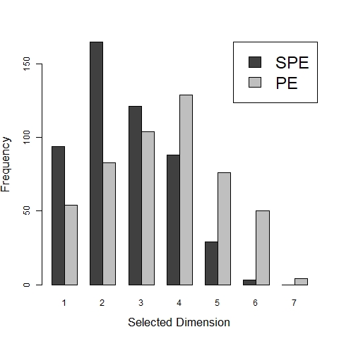
Refer to caption
(a) n=50𝑛50n=50
Refer to caption
(b) n=100𝑛100n=100
Refer to caption
(c) n=200𝑛200n=200
Figure 4: Histograms of estimated envelope dimensions for Simulation 2: u<p𝑢𝑝u<p and 𝛀0𝛀1much-less-thannormsubscript𝛀0normsubscript𝛀1\|\bm{\Omega}_{0}\|\ll\|\bm{\Omega}_{1}\|.
Refer to caption
(a) n=50𝑛50n=50
Refer to caption
(b) n=100𝑛100n=100
Refer to caption
(c) n=200𝑛200n=200
Figure 5: Histograms of estimated envelope dimensions for Simulation 3: u=p𝑢𝑝u=p.
Refer to caption
(a) n=50𝑛50n=50
Refer to caption
(b) n=100𝑛100n=100
Refer to caption
(c) n=200𝑛200n=200
Figure 6: Histograms of estimated envelope dimensions for Simulation 4: u<p𝑢𝑝u<p and 𝛀1𝛀0normsubscript𝛀1normsubscript𝛀0\|\bm{\Omega}_{1}\|\approx\|\bm{\Omega}_{0}\|.

8.5 Data Analysis

Traditional multivariate techniques cannot be directly applied to compositional data because of the variable constraints: all variables for a given observation sum to unity. Thus, it has become common to analyze the log-ratios of the components. Let Z=[Z1,,Zk]𝑍subscript𝑍1subscript𝑍𝑘\vec{Z}=[Z_{1},\ldots,Z_{k}] be a k𝑘k-dimensional composition (or subcomposition). Then the k1𝑘1k-1 dimensional transformed variable

X=[log(Z1/Zk)log(Z2/Zk)log(Zk1/Zk)]T,𝑋superscriptdelimited-[]subscript𝑍1subscript𝑍𝑘subscript𝑍2subscript𝑍𝑘subscript𝑍𝑘1subscript𝑍𝑘𝑇\vec{X}=[\log(Z_{1}/Z_{k})\ \log(Z_{2}/Z_{k})\ \cdots\ \log(Z_{k-1}/Z_{k})]^{T},

is unconstrained. Furthermore, if the composition Z𝑍\vec{Z} is assumed to follow a logistic normal distribution, then X𝑋\vec{X} follows a multivariate normal distribution. The choice of denominator in the ratio, given above as the last component of the composition, is arbitrary, and equivalent inference is obtained for any choice of denominator (Aitchison, 1982, Chapter 5).

For the data analysis in this paper, the predictors were chosen to be the relative log-concentrations of the major chemical elements. Let MCE1,,MCE11subscriptMCE1subscriptMCE11\text{MCE}_{1},\ldots,\text{MCE}_{11} represent the eleven major chemical elements. The major chemical elements are examined as a subcomposition, with

Zj=MCEj/(w=111MCEw),subscript𝑍𝑗subscriptMCE𝑗superscriptsubscript𝑤111subscriptMCE𝑤Z_{j}=\text{MCE}_{j}/(\sum_{w=1}^{11}\text{MCE}_{w}),

normalizing so that the relative proportions of the major chemical elements are studied. The major chemical elements are normalized as a separate subcompositon in order to remove any trivial, compositional relationships between the predictors and the response, for example, an increase in potassium oxide concentration causes a decrease in REE concentration simply by leaving less room in the composition. Rather, the goal is to analyze the effect of the relative proportions of major chemical elements on the REE concentration, for example, in increase in potassium oxide relative to the other major chemical elements makes higher REE concentrations likely. To remove the constraints on the predictors, a log-ratio transformation is applied

Xj=log(Zj/Z11),j=1,,10formulae-sequencesubscript𝑋𝑗subscript𝑍𝑗subscript𝑍11𝑗110X_{j}=\log(Z_{j}/Z_{11}),\ j=1,\ldots,10

leaving p=10𝑝10p=10 predictor variables, with major chemical element aluminum oxide (Al2O3) arbitrarily chosen as the denominator.

The REE element concentrations are represented in parts per million, between 00 and 106superscript10610^{6}. The regression response is chosen to be the log-concentration of REEs relative to all other parts of the composition

Y=log(REE/(106REE)).𝑌𝑅𝐸𝐸superscript106𝑅𝐸𝐸Y=\log(REE/(10^{6}-REE)).

a monotone increasing transformation that gives a response that is unconstrained, interpretable and congruent with the goals of the analysis.

Some of the observations had chemical element concentrations below the detection threshold of the instrument used to analyze the sample. Specifically, three samples had a major chemical element titanium dioxide (TiO2) below the detection threshold and ten samples had at least one rare earth element below the detection threshold. Rather than omit these samples, the values were replaced with half of the detection threshold. Because so few samples had a major chemical element below the detection threshold, and any REE below the detection threshold will have little impact on the total REE concentration, this choice of replacement had little impact when compared to any other reasonable replacement scheme.