subsecref subsecname = thmref thmname = theorem  lemref lemname = lemma  20 thmname=theorem ,Name=Theorem ,names=theorems ,Names=Theorems  defname=definition ,Name=Definition ,names=definitions ,Names=Definitions  corname=corollary ,Name=Corollary ,names=corollaries ,Names=Corollaries  lemname=lemma ,Name=Lemma ,names=lemmas ,Names=Lemmas  claimname=claim ,Name=Claim ,names=claims ,Names=Claims  secname=section ,Name=Section ,names=sections ,Names=Sections  subsecname=subsection ,Name=Subsection ,names=subsections ,Names=Subsections  propname=proposition ,Name=Proposition ,names=propositions ,Names=Propositions  remname=remark ,Name=Remark ,names=remarks ,Names=Remarks  algname=algorithm ,Name=Algorithm ,names=algorithms ,Names=Algorithms  notename=note ,Name=Note ,names=notes ,Names=Notes  notaname=notation ,Name=Notation ,names=notations ,Names=Notations  exaname=example ,Name=Example ,names=examples ,Names=Examples  tabname=table ,Name=Table ,names=tables ,Names=Tables 

Oracle separations of hybrid quantum-classical circuits

An important theoretical problem in the study of quantum computation, that is also practically relevant in the context of near-term quantum devices, is to understand the computational power of hybrid models, that combine polynomial-time classical computation with short-depth quantum computation. Here, we consider two such models: $\mathsf{CQ_{d}}$ which captures the scenario of a polynomial-time classical algorithm that queries a $d$-depth quantum computer many times; and $\mathsf{QC_{d}}$ which is more analogous to measurement-based quantum computation and captures the scenario of a $d$-depth quantum computer with the ability to change the sequence of gates being applied depending on measurement outcomes processed by a classical computation. Chia, Chung and Lai (STOC 2020) and Coudron and Menda (STOC 2020) showed that these models (with $d=\log^{\mathcal{O}(1)}(n)$) are strictly weaker than $\mathsf{BQP}$ (the class of problems solvable by polynomial-time quantum computation), relative to an oracle, disproving a conjecture of Jozsa in the relativised world.

In this paper, we show that, despite the similarities between $\mathsf{CQ_{d}}$ and $\mathsf{QC_{d}}$, the two models are incomparable, i.e. $\mathsf{CQ_{d}}\not\subseteq\mathsf{QC_{d}}$ and $\mathsf{QC_{d}}\not\subseteq\mathsf{CQ_{d}}$ relative to an oracle. In other words, we show that there exist problems that one model can solve but not the other and vice versa. We do this by considering new oracle problems that capture the distinctions between the two models and by introducing the notion of an intrinsically stochastic oracle, an oracle whose responses are inherently randomised, which is used for our second result. While we leave showing the second separation relative to a standard oracle as an open problem, we believe the notion of stochastic oracles could be of independent interest for studying complexity classes which have resisted separation in the standard oracle model. Our constructions also yield simpler oracle separations between the hybrid models and $\mathsf{BQP}$, compared to earlier works.

1 Introduction

One of the major goals of modern complexity theory is understanding the relations between various models of efficient quantum computation and classical computation. It is widely believed that the set of problems solvable by polynomial-time quantum algorithms, denoted $\mathsf{BQP}$, is strictly larger than that solvable by polynomial-time classical algorithms, denoted $\mathsf{BPP}$ [BV97, Sho97, Aru+19]. This, so-called Deutsch-Church-Turing thesis, is motivated by the existence of a number of problems which seem to be classically intractable, but which admit efficient (polynomial-time) quantum algorithms. Notable examples include period finding [Sim97], integer factorisation [Sho97], the discrete-logarithm problem [Sho97], solving Pell’s equation [Hal02], approximating the Jones polynomial [AJL06] and others [Jor]. In a seminal paper of Cleve and Watrous [CW00], it was shown that many of these problems (period finding, factoring and discrete-logarithm) can also be solved by quantum circuits of logarithmic-depth together with classical pre- and post-processing. In the language of complexity theory, we say that these problems are contained in the complexity class $\mathsf{BPP}^{\mathsf{QNC}}$. This motivated Jozsa to conjecture that $\mathsf{BPP}^{\mathsf{QNC}}=\mathsf{BQP}$ [Joz06]. In other words, it was conjectured that the computational power of general polynomial-size quantum circuits is fully captured by quantum circuits of polylogarithmic depth (the class $\mathsf{QNC}$) together with classical pre- and post-processing.

In fact, Jozsa’s conjecture was more broad than simply asserting that $\mathsf{BPP}^{\mathsf{QNC}}=\mathsf{BQP}$. To explain why, one needs to distinguish between two hybrid models of classical computation and short-depth quantum computation. These two models capture the idea of interleaving polynomial-time classical computations with $d$-depth quantum computations. The first model, denoted $\mathsf{CQ_{d}}$, refers to polynomial-time classical circuits that can call $d$-depth quantum circuits, as a subroutine, and use their output (see LABEL:Fig:CQd). This is analogous to $\mathsf{BPP}^{\mathsf{QNC}}$, except the quantum circuits are of depth $d$ rather than $\log^{O(1)}(n)$ (where $n$ is the size of the input). The second model, denoted $\mathsf{QC_{d}}$, refers to $d$-depth quantum circuits that can, at each circuit layer, call polynomial-time classical circuits, as a subroutine and use their output (see LABEL:Fig:QCd). Importantly, the classical circuits cannot be invoked coherently—part of the quantum state produced by the circuit is measured and the classical subroutine is invoked on the classical outcome of that measurement.

Though $\mathsf{CQ_{d}}$ and $\mathsf{QC_{d}}$ circuits seem similar, they both capture different aspects of short-depth quantum computation together with polynomial-time classical computation. $\mathsf{CQ_{d}}$ captures the scenario of a classical algorithm that queries a short-depth quantum computer many times, while $\mathsf{QC_{d}}$ is more analogous to measurement-based quantum computation in that it captures a short-depth quantum computer with the ability to change the sequence of gates being applied depending on measurement outcomes processed by a classical computation.

Jozsa’s conjecture is the assertion that the power of $\mathsf{BQP}$ is fully captured by logarithmic-depth quantum computation interspersed with polynomial-depth classical computation. This can be interpreted either as $\mathsf{BQP}=\mathsf{CQ_{d}}$ or $\mathsf{BQP}=\mathsf{QC_{d}}$ with $d=\log^{O(1)}(n)$. Aaronson later proposed as one of his “ten semi-grand challenges in quantum complexity theory” to find an oracle separation between $\mathsf{BQP}$ and the two hybrid models [Aar05]. That is, to provide an oracle $O$ and a problem defined relative to this oracle which is contained in $\mathsf{BQP}^{O}$ but not in $\mathsf{QC_{d}}^{O}$ or $\mathsf{CQ_{d}}^{O}$. This was resolved in the landmark works of Chia, Chung and Lai [CCL20] and, independently, Coudron and Menda [CM20]. They showed that indeed such an oracle exists and also proved a hierarchy theorem for the two hybrid models showing that $\mathsf{QC_{d}}^{O}\subsetneq\mathsf{QC_{d^{\prime}}}^{O}$ and $\mathsf{CQ_{d}}^{O}\subsetneq\mathsf{CQ_{d^{\prime}}}^{O}$, whenever $d^{\prime}=2d+1$. However, both works left it as an open problem whether there exists an oracle separation between $\mathsf{QC_{d}}$ and $\mathsf{CQ_{d}}$.

1.1 Contributions

In our work, we resolve this question by showing that, indeed, there exist oracles $O_{1}$ and $O_{2}$ such that $\mathsf{QC_{d}}^{O_{1}}\not\supseteq\mathsf{CQ_{d}}^{O_{1}}$ and $\mathsf{CQ_{d}}^{O_{2}}\not\supseteq\mathsf{QC_{d}}^{O_{2}}$. In other words, the two hybrid models are incomparable—there exist problems that one can solve but not the other and vice versa. As corollaries, we also obtain simpler oracle constructions for separating the two hybrid models from $\mathsf{BQP}$. It’s important to note that for our results $O_{1}$ is a standard oracle, i.e. one that performs the mapping $\ket{x}\ket{z}\overset{O_{1}}{\to}\ket{x}\ket{z\oplus f(x)}$, for some function $f:X\to Z$. However, the oracle $O_{2}$ is one which we refer to as an intrinsically stochastic oracle, which is defined for a function $f:X\times Y\to Z$ and a probability distribution $\mathbb{F}_{Y}$ over $Y$. Classically, for each query $x\in X$, it samples a new $y\sim\mathbb{F}_{Y}$ and returns $f(x,y)$. Quantumly, for every application, it samples a new $y\sim\mathbb{F}_{Y}$ and performs the mapping $\ket{x}\ket{z}\overset{O_{2}}{\to}\ket{x}\ket{z\oplus f(x,y)}$.

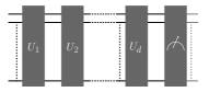
(a) ${\rm QNC}_{d}$ scheme; $U_{i}$ are single depth unitaries; $\Pi$ is a projector in the computational basis.

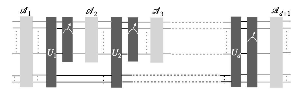
(b) ${\rm QC}_{d}$ circuit; $U_{i}$ are single layered unitaries, $\mathcal{A}_{c,i}$ are classical poly-sized circuits (in the figure, the subscript for $\mathcal{A}_{c}$ has been dropped) and the measurements are in the computational basis. Dark lines denote qubits.

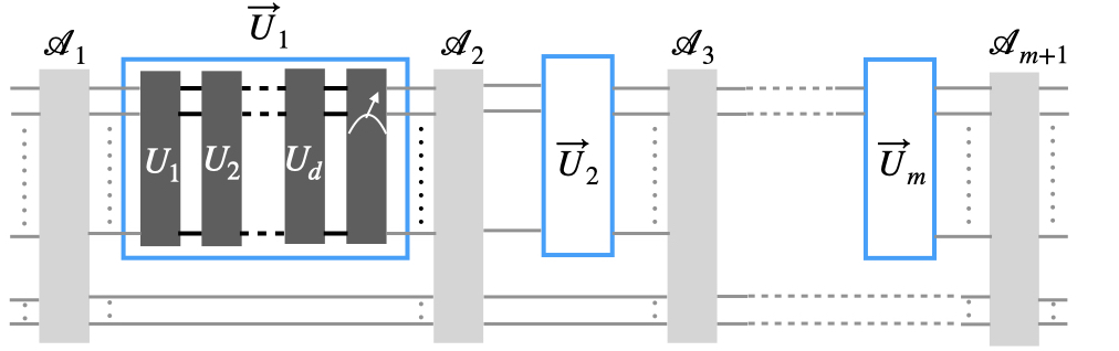
(c) ${\rm CQ}_{d}$ circuit; for clarity, we dropped the indices in $\mathcal{A}_{c}$ and the second indices in $U_{1,i},U_{2,i}\dots U_{d,i}$.

Figure 1: The three circuit models we consider.

	$\mathsf{QC_{d}}$	$\mathsf{CQ_{d}}$	Oracle Model
$d^{\prime}$-SeS	$d^{\prime}+1\leq d\leq 2d^{\prime}+2$	$d\leq 1$	Standard	This work
$d^{\prime}$-SCS	$d\leq 4$	$d^{\prime}+1\leq d\leq d^{\prime}+5$	Stochastic	This work
$d^{\prime}$-SSP	$d^{\prime}+1\leq d\leq 2d^{\prime}+2$	$d^{\prime}+1\leq d\leq 2d^{\prime}+1$	Standard	CCL

Table 1: Summary of our results: bounds on the smallest depth, $d$, needed to solve $d^{\prime}$-Serial Simon’s ($d^{\prime}$-SeS) Problem and $d^{\prime}$-Shuffled Collisions-to-Simon’s ($d^{\prime}$-SCS) Problem in the two hybrid models of computation compared to those of $d^{\prime}$-Shuffling Simon’s Problem ($d^{\prime}$-SSP) introduced by CCL.

We summarise our main results in main. In particular, we obtain our first result by introducing an oracle problem that we call the $d$-Serial Simon’s ($d$-SeS) Problem, which lets us show the following:

Theorem 1 (informal).

There exists a standard oracle, $O$, such that for all $d>0$, $\mathsf{QC_{d}}^{O}\not\supseteq\mathsf{CQ_{d}}^{O}.$

Intuitively, since $\mathsf{CQ_{d}}$ can perform polynomially-many calls to a $d$-depth quantum circuit, we’d like to define a problem which forces one to sequentially solve $d$ Simon’s problems. In other words, the period of each Simon’s function can be viewed as a key which unlocks in the oracle a different Simon function. The $d$-SeS problem is to find the period of the $d$’th function. This problem can be solved in $\mathsf{CQ}_{1}$, since the poly-time algorithm can invoke $d$ separate constant-depth quantum circuits to solve each Simon problem. However, due to the serial nature of the problem, we show that no $\mathsf{QC_{d}}$ algorithm can succeed.

For our second separation, we consider a problem we call the $d$-Shuffled Collisions-to-Simon’s ($d$-SCS) Problem and show that:

Theorem 2 (informal).

There exists an intrinsically stochastic oracle, $O$, such that for all $d\geq 4$, $\mathsf{CQ_{d}}^{O}\not\supseteq\mathsf{QC_{d}}^{O}$.

This separation is perhaps more surprising because $\mathsf{QC_{d}}$ has only $d$ quantum layers while $\mathsf{CQ_{d}}$ has polynomially-many quantum layers (as it can invoke $d$-depth quantum circuits polynomially-many times). Importantly, however, in $\mathsf{CQ_{d}}$ the quantum states prepared when invoking a $d$-depth quantum circuit are measured entirely. In contrast, in $\mathsf{QC_{d}}$ some qubits are measured and the outcomes are sent to a classical subroutine, while other qubits remain unmeasured and maintain their coherence in between the layers of classical computation. This observation is the basis for defining $d$-SCS, which can still be viewed as a version of Simon’s problem, in which one has to find a secret period $s$. To explain the idea, we briefly recap the textbook quantum algorithm for Simon’s problem. One first queries the oracle to the Simon function in superposition to obtain the state $\sum_{x}\ket{x}\ket{g(x)}$, where $g:\{0,1\}^{n}\to\{0,1\}^{n}$ is the Simon function, with period $s\in\{0,1\}^{n},s\neq 0^{n}$. The second register is then measured, yielding

$$\frac{1}{\sqrt{2}}(\ket{x}+\ket{x\oplus s})\ket{y}$$ (1)

with $y=g(x)=g(x\oplus s)$. Finally, by applying Hadamard gates and measuring the first register, one obtains a string $w\in\{0,1\}^{n}$, such that $w\cdot s=0$. Repeating this in parallel $O(n)$ times yields a system of linear equations from which $s$ can be uniquely recovered.

Note that in Simon’s algorithm, the main component of the quantum algorithm is to generate superpositions over colliding pre-images (i.e. pre-images that map to the same image). For $d$-SCS, a first difference with respect to the standard Simon’s problem is that the oracle doesn’t provide direct access to the Simon function $g$. Instead, consider three functions: a random 2-to-1 function, $f$, a function $p$ which maps colliding pairs of $f$ to those of $g$ and the inverse of $p$. Since $f$ and $g$ are both $2$-to-1, $p$ is a bijection and its inverse is well defined. If one is given access to all three functions, then evidently, the problem is equivalent to that of Simon’s: the quantum algorithm would create superpositions over colliding pairs of $f$ and then coherently evaluate the bijection together with its inverse, to obtain superpositions over colliding pairs of $g$. To obtain the desired separation—a problem that $\mathsf{QC_{d}}$ can solve but $\mathsf{CQ_{d}}$ cannot—we only allow restricted access to the bijection $p$. This restriction, denoted $p^{\prime}$, may be seen as a form of encrypted access to $p$. Specifically, to evaluate the bijection (or its inverse) $p$ on a colliding pair $(x_{0},x_{1})$ of $f$, i.e. $f(x_{0})=f(x_{1})=y$, $p^{\prime}$ additionally takes a “key” $h(y)$ as input. Access to the function $h,$which produces the key $h(y)$, is also restricted. It is given via a shuffler $\Xi$—an encoding which ensures that at least depth $d$ is required to evaluate $h$.

So far, given access to $f$, $p^{\prime}$ (which encodes $p$) and $\Xi$ (which encodes $h$), the goal is to find $s$ (the period of $g$). It is easy to see that a ${\rm QC}_{4}$ algorithm can solve this problem. The algorithm first creates equal superpositions of colliding pairs for $f$ as in Simon’s algorithm. The measured image register, which now contains the classical value $f(x_{0})=f(x_{1})=y$, can be used to evaluate $h(y)$ via $\Xi$ by expending $d$ classical depth. The ${\rm QC}_{4}$ circuit can perform this computation—it can perform poly depth classical computation while maintaining quantum coherence. With $h(y)$ known, in a second quantum layer, the bijection (and its inverse) $p$ is evaluated, via $p^{\prime}$, on the superposition of colliding pairs $\left|x_{0}\right\rangle+\left|x_{1}\right\rangle$ to obtain $\left|p(x_{0})\right\rangle+\left|p(x_{1})\right\rangle$ (up to normalisation). Recalling that $(p(x_{0}),p(x_{1}))$ are pre-images of the Simon function $g$, it only remains to make Hadamard measurements to obtain the system of linear equations which yield the secret $s$.

Why can’t a $\mathsf{CQ_{d}}$ algorithm also solve this problem? By making the oracle provide access to a generic $2$-to-$1$ function, $f$, instead of the Simon function, we made it so that superpositions over colliding pairs are no longer related by the period $s$. Indeed, the only way to obtain any information about $s$ is to query the bijection. But in the case of $\mathsf{CQ_{d}}$ the quantum subroutines must measure their states completely before invoking the classical subroutines. This means that the quantum subroutines essentially obtain no information about $s$. We also know that only the classical subroutines can obtain access to the bijection as the shuffler can only be invoked by a circuit of depth at least $d$. In essence, we’ve made it so that if a $\mathsf{CQ_{d}}$ algorithm could solve the problem with a polynomial number of oracle queries, then Simon’s problem could also be solved classically with a polynomial number of queries, which we know is impossible.

Formalising the above intuition turns out to be surprisingly involved. This is due to the following subtlety: the classical subroutines of $\mathsf{CQ_{d}}$ can obtain some information about $g$ by querying the bijection (essentially obtaining evaluations of $g$) and one would have to show that this information is insufficient for recovering $s$ even when invoking short depth quantum subroutines. We overcome this barrier by using a stochastic oracle in our proof but nevertheless conjecture that the result should also hold in the standard oracle setting. Thus, our final modification to Simon’s problem, leading to the definition of $d$-SCS is to make it so that the oracle does not even provide direct access to $f$ but instead, given a single bit as input, performs the following mappings:

$$0\stackrel{{\scriptstyle\mathcal{S}}}{{\to}}(x_{0},f(x_{0})),\quad 1\stackrel{{\scriptstyle\mathcal{S}}}{{\to}}(x_{1},f(x_{1}))$$ (2)

where $(x_{0},x_{1})$ is a randomly chosen colliding pair of $g$. In other words, the oracle picks a random colliding pair for $g$ and outputs either the first element in the pair or the second, depending on whether the input was $0$ or $1$. In the quantum setting, this translates to

$$\ket{0}_{\mathsf{{B}}}\ket{0}_{\mathsf{{X}}}\ket{0}_{\mathsf{{Y}}}\overset{\mathcal{S}}{\to}\ket{0}_{\mathsf{{B}}}\ket{x_{0}}_{\mathsf{{X}}}\ket{f(x_{0})}_{\mathsf{{Y}}}$$ (3)

$$\ket{1}_{\mathsf{{B}}}\ket{0}_{\mathsf{{X}}}\ket{0}_{\mathsf{{Y}}}\overset{\mathcal{S}}{\to}\ket{1}_{\mathsf{{B}}}\ket{x_{1}}_{\mathsf{{X}}}\ket{f(x_{1})}_{\mathsf{{Y}}}$$ (4)

We can therefore see that if the input qubit is in an equal superposition of $\ket{0}$and $\ket{1}$ (while all other registers are initialised as $\ket{0}$) we would obtain the state

$$\frac{1}{\sqrt{2}}(\ket{0}_{\mathsf{{B}}}\ket{x_{0}}_{\mathsf{{X}}}+\ket{1}_{\mathsf{{B}}}\ket{x_{1}}_{\mathsf{{X}}})\ket{f(x_{0})=f(x_{1})}_{\mathsf{{Y}}}$$ (5)

This is the same type of state as that of Equation 1, except the superposition is over pre-images of $f$ rather than the Simon function $g$. The oracle will still provide access to the bijection and the shuffler in the manner explained above, so that the stochastic access to $f$ does not change the fact that a $\mathsf{{QC}_{4}}$ algorithm is still able to solve the problem (one is still able to map these states to superpositions over colliding pairs of $g$). But this stochastic access further restricts what a $\mathsf{CQ_{d}}$ algorithm can do, as now even if the classical subroutines are used to obtain evaluations of $g$, the stochastic nature of the oracle guarantees that these evaluations are uniformly random points. With this restriction in place, one can then show that $\mathsf{CQ_{d}}$ cannot solve the problem unless Simon’s problem can be solved classically with polynomially-many queries.

1.2 Overview of the techniques

We begin with sketching the idea behind the hardness of $d$-SeS for $\mathsf{QC_{d}}$ circuits. To this end, we first describe the $d$-SeS problem in some more detail.

The $d$-Serial Simon’s Problem (informal).

Sample $d+1$ random Simon’s functions $\{f_{i}\}_{i=0}^{d}$ with periods $\{s_{i}\}_{i=0}^{d}$. The problem is to find the period, $s_{d}$, of the last Simon’s function. However, only access to $f_{0}$ is given directly. Access to $f_{i}$, for $i\geq 1$, is given via a function $L_{f_{i}}$ which outputs $f_{i}(x)$ if the input is $(s_{i-1},x)$ and $\perp$ otherwise, i.e. to access the $i$th Simon’s function, one needs the period of the $(i-1)$th Simon’s function (see LABEL:Def:cSerialSimonsOracle and LABEL:Def:cSerialSimonsProblem for details).

The lower bound technique.

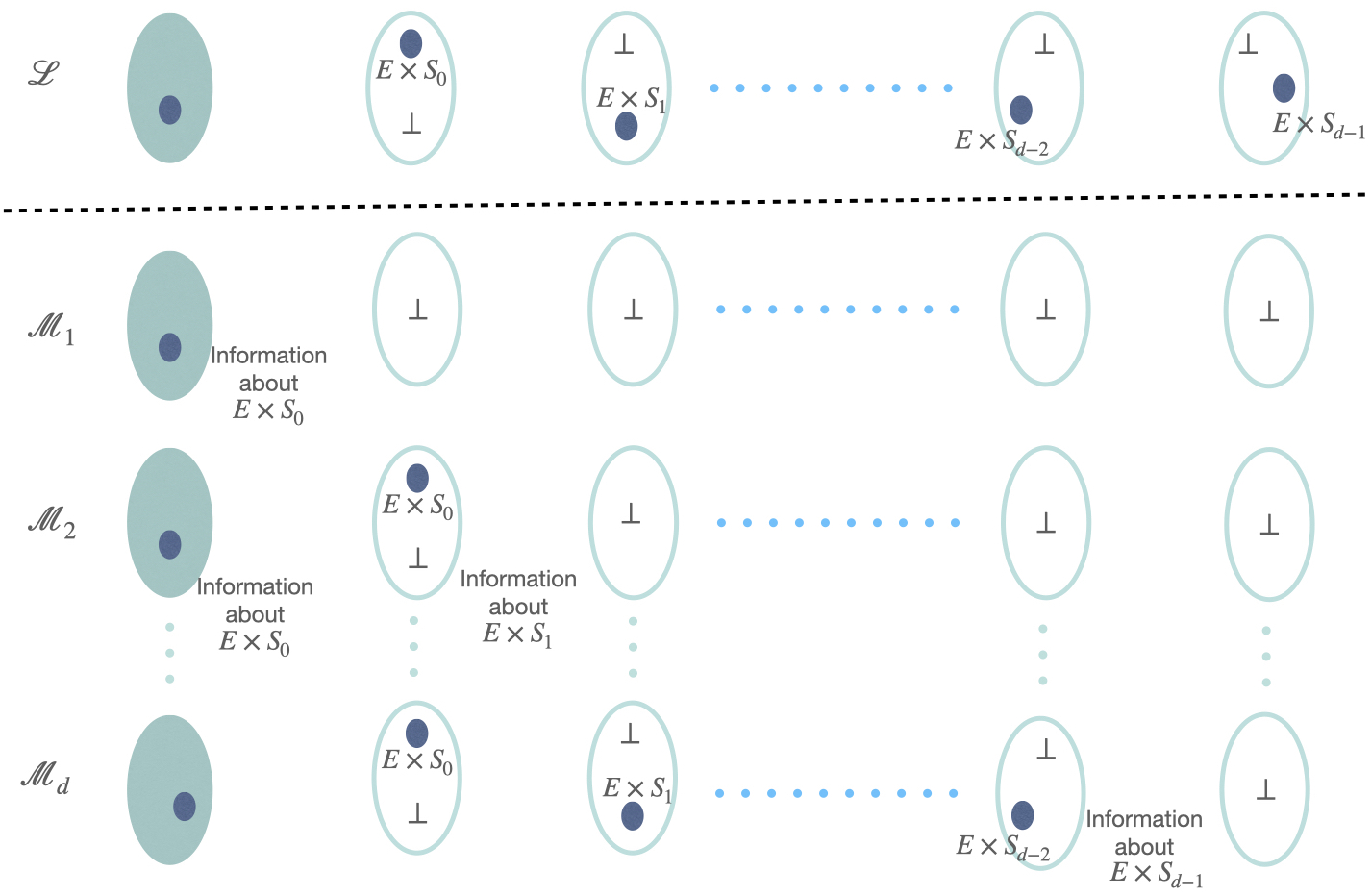
Figure 2: Shadows for ${\rm QNC}_{d}$. The ovals represent the query domains of the various sub-oracles. Shaded regions denote a non-$\perp$ response. Let $\bar{S}_{i}$ denote the query domain at which $\mathcal{L}$ and $\mathcal{M}_{i}$ differ. The construction ensures that $\mathcal{M}_{1},\dots\mathcal{M}_{i-1}$ contain no information about $\bar{S}_{i}$. Convention: The left-most sub-oracles are numbered zero (and they respond with non-$\perp$ on $\{0,1\}^{n}$).

We now sketch the idea behind the proof that $\mathsf{QC_{d}}$ circuits solve $d$-SeS with at most negligible probability (see LABEL:Sec:-Serial-Simon's-Problem). Denote the initial set of oracles by $\mathcal{L}$. Let $\mathcal{M}_{i}$, for $1\leq i\leq d$, be identical to $\mathcal{L}$, except the oracles $i,\dots d$ output $\perp$ at all inputs (see LABEL:Fig:ShadowsQNCd). Using a hybrid argument, we show that the $d$-depth quantum circuit $\mathcal{C}:=U_{d+1}\circ\mathcal{L}\circ U_{d}\dots\mathcal{L}\circ U_{1}$ behaves essentially like $U_{d+1}\circ\mathcal{M}_{d}\circ U_{d}\dots\mathcal{M}_{1}U_{1}$. The intuition is that since all $s_{i}$ are unknown before the oracles are invoked, the domain at which the oracles respond non-trivially (i.e. $\neq\perp$) is hard to find. After $\mathcal{M}_{i-1}$ is invoked, the “non-trivial domain” of the $i$th oracle can be learnt. It is therefore exposed in $\mathcal{M}_{i}$. Evidently, since $\mathcal{M}_{1},\dots\mathcal{M}_{d}$ do not contain any information about $f_{d}$, we conclude the $d$-depth quantum circuit $\mathcal{C}$ cannot solve $d$-SeS with non-negligible probability. The conclusion continues to hold even when efficient classical computation is allowed between the unitaries. At a high level, this is because one can condition on the classical queries yielding $\perp$ and show that this happens with high probability. Since only polynomially many queries are possible, the aforementioned analysis goes through largely unchanged. This proof is quite straightforward and consequently also serves as a considerable simplification of the proof of the $\mathsf{QC_{d}}$ depth hierarchy theorem proved by CCL.

 

We now turn to the ideas behind the hardness of the $d$-SCS problem for $\mathsf{CQ_{d}}$ circuits. We describe the $d$-SCS problem in some detail and to this end, first introduce the $d$-Shuffler construction which is used for enforcing statements like “$k$ is a function which requires depth larger than $d$ to evaluate”.

The $d$-Shuffler (informal).

Intuitively, a $d$-Shuffler is an oracle which encodes a function, say $f:\{0,1\}^{n}\to\{0,1\}^{n}$, in such a way that one needs to make $d$ sequential calls to it, to access $f$. Consider $d$ random permutations, $f^{\prime}_{0},f^{\prime}_{1}\dots f^{\prime}_{d-1}$, from $\{0,1\}^{2n}\to\{0,1\}^{2n}$. Define $f^{\prime}_{d}$ to be such that $f^{\prime}_{d}(f^{\prime}_{d-1}\dots f^{\prime}_{0}(x))\dots)=f(x)$ for $x\in\{0,1\}^{n}$. Define $f_{i}$, for $0\leq i\leq d$, to be $f^{\prime}_{i}(f^{\prime}_{i-1}(\dots f^{\prime}_{0}(x)\dots))$ for $x\in\{0,1\}^{n}$ and $\perp$ otherwise. We say $(f_{i})_{i=0}^{d}$ is the $d$-Shuffler encoding $f$. We also use $\Xi$ to abstractly refer to it. Using an argument, similar to the one above, one can show that no $d$-depth quantum circuit can access $f$ via a $d$-Shuffler, with non-negligible probability (see LABEL:Def:dShuffler).

The $d$-Shuffled Collisions-to-Simon’s Problem (informal).

Consider the following functions on $n$-bit functions. Uniformly sample $f$ from all 2-to-1 functions, $g$ from all Simon’s functions, and $h$ from all $1$-to-$1$ functions. Let $p$ be some canonical bijection which maps colliding pairs of $f$ to those of $g$ (and $p_{{\rm inv}}$ be the inverse).

Let $p^{\prime}$ be such that $p^{\prime}(h(f(x)),x)=p(x)$ and $\perp$ if the input is not of that form ($p^{\prime}_{{\rm inv}}$ is similarly defined). Let $\Xi$ be a $d$-Shuffler encoding $h$. The problem is, given access to $\mathcal{S}$ (a stochastic oracle, encoding $f$ as in LABEL:Eq:S), $p^{\prime}$, $p^{\prime}_{{\rm inv}}$ and $\Xi$, find the period $s$ of $g$.

The lower bound technique.

We briefly outline the broad argument for why $\mathsf{CQ_{d}}$ circuits can solve $d$-SCS with at most negligible probability (see LABEL:Sec:ShuffledCollisionsToSimons). Consider the first classical circuit: It has vanishing probability of learning a collision from $\mathcal{S}$ (since $y$ is chosen stochastically). So, with overwhelming probability, it can learn at most polynomially many values of $p,p_{{\rm inv}}$, $h$ and non colliding values of $f$.

For the subsequent quantum circuit, we expose those values in the shadows of $p^{\prime},p^{\prime}_{{\rm inv}}$ and $\Xi$ (a $d$-Shuffler which encodes $h$). Here shadows are the analogues of $\mathcal{M}_{i}$ introduced above. For $\mathcal{S}$, we condition on never seeing the $y$s which already appeared (this will happen with overwhelming probability). Without access to $h$ for the new $y$ values (since access to $h$ is via $\Xi$ which requires at least depth $d$), the circuit cannot distinguish the shadows of $p^{\prime},p^{\prime}_{{\rm inv}}$ from the originals; the shadows contain no information about $s$ (informally, they could contain $z$ or $z\oplus s$ but not both). Finally, since $f$ is a random two-to-one function, and since it is known that finding collisions even when given direct oracle access to $f$ is hard, the quantum output cannot contain collisions (with non-negligible probability).

The next classical circuit, did not learn of any collisions from the quantum output. Further, it did not learn anything about the function, other than those which evaluate to $y$s which appeared in the previous step. Conditioned on the same $y$s not appearing (which happens with overwhelming probability), we can repeat the reasoning from the first step, polynomially many times.

In the proof, we first show that one can replace the oracles with their shadows, without changing the outputs of the circuits noticeably. We then show that if no collisions are revealed, the shadows contain no information about $s$ and that collisions are revealed with negligible probability. For the full details of the proofs we refer the reader to LABEL:Sec:ShuffledCollisionsToSimons.

1.3 Organisation

We begin with introducing the precise models of computation we consider in LABEL:Sec:Models-of-Computation, followed by brief statements of the basic results in query complexity which we use, in LABEL:Sec:Prerequisite-Technical-Results. Our first main result—that $d$-Serial Simon’s Problem can be solved using $\mathsf{CQ_{1}}$ while it is hard for $\mathsf{QC_{d}}$—is established in LABEL:Sec:-Serial-Simon's-Problem. The second main result, however, requires more ground work. We first study the simpler aspects of the $d$-Shuffled Simon’s problem in LABEL:Sec:warm-up-dSS where we introduce the $d$-Shuffler (a close variant of the $d$-Shuffling technique introduced by CCL). In LABEL:Sec:Technical-Results-II we generalise the so-called “sampling argument” as formulated by CCL, which may be of independent interest. It is a technique used for establishing the continued utility of $d$-Shufflers despite repeated applications. We give a new proof of hardness of $d$-SS for $\mathsf{CQ_{d}}$ circuits in LABEL:Sec:dSS_hard_2 and use this as an intermediate step for the proof of our second main result which is delineated in LABEL:Sec:ShuffledCollisionsToSimons. This final section begins with formalising intrinsically stochastic oracles, defines the $d$-SCS problem precisely, gives the algorithms for establishing the upper bounds and concludes with the proof hardness for $\mathsf{CQ_{d}}$.

1.4 Relation to Prior Work

Four connections with [CCL20] are noteworthy.

First, as was already noted, we recover the depth hierarchy for $\mathsf{QC_{d}}$ with less effort. This was done by circumventing the use of the $d$-Shuffling and the “Russian nesting doll” technique employed by CCL. Our result is, in fact, slightly stronger too since if we allow Hadamard measurements in the $\mathsf{QC_{d}}$ model, our hierarchy theorem becomes optimal, i.e. it separates $d$ and $d+1$ depth. This was one of their open questions, as their separation was between $d$ and $2d+1$, even if we allow Hadamard measurements.

Second, we give a new proof of hardness of $d$-SS for $\mathsf{CQ_{d}}$. This proof is arguably simpler in that while it uses ideas related to $d$-Shuffling, it does not rely on the “Russian nesting doll” technique. Aside from simplicity, the information required to specify the oracles in the proof by CCL scaled exponentially with $d$ while in our proof, there is no dependence on $d$.

Third, the connection between the “sampling argument”, the $d$-Shuffler and $d$-Shuffling. We show that the “sampling argument” as used by CCL holds quite generally and in doing so, obtain a proof which relies on very simple properties of the underlying distribution. We also show a composition result which allows us to repeatedly use the argument. We use this generalisation to establish the utility of the $d$-Shuffler.

Fourth, we also get a hierarchy theorem for $\mathsf{CQ_{d}}$ based on the hardness of the $d$-SCS problem. While this hierarchy theorem holds in the stochastic oracle setting and is thus not as strong as that obtained using $d$-SS (or $d$-Shuffling Simon’s problem) which holds in the standard oracle setting, nevertheless, it yields a finer separation—it separates $d$ from $d+5$.

1.5 Conclusion and Outlook

In addition to resolving the open problems left by the works of [CCL20] and [CM20], our results provide additional insights into the relations between different models of hybrid classical-quantum computation and sharpen our understanding of these models. Specifically, we find that $\mathsf{QC_{d}}$ and $\mathsf{CQ_{d}}$ solve incomparable sets of problems. Our results relativise and so one should obtain a similar conclusion about a hierarchy of analogous classes ($\mathsf{QCQC..QC_{d}}$, $\mathsf{CQC..CQ_{d}}$ etc). While an important open problem is whether the stochastic oracle in our second construction can be replaced with a standard oracle, we speculate that other classes which have resisted separation in the standard oracle model, may also admit separations via stochastic oracles.

A potentially interesting application that is hinted by our work, assuming the oracles can be instantiated with cryptographic primitives, is that of tests of coherent quantum control. In other words, the idea is to design a task (or a test) which can be solved by a quantum device having coherent control (the ability to adapt the gates it will perform based on the measurement results) but which cannot be solved by a device without coherent control (one which performs a measurement of all its qubits when providing a response). This is related to the recent notion of proofs of quantumness [Bra+18, Bra+20]. This is a test which can be passed by a $\mathsf{BQP}$ machine but not by a $\mathsf{BPP}$ one, assuming the intractability of some cryptographic task. In a test of coherent control, the tester (or verifier) has the ability to check for a more fine-grained notion of “quantumness” on the part of the quantum device (prover) and not just its ability to solve, say, $\mathsf{BQP}$ problems.

1.6 Acknowledgements

AG is supported by Dr. Max Rössler, the Walter Haefner Foundation and the ETH Zürich Foundation. ASA acknowledges funding provided by the Institute for Quantum Information and Matter. We are thankful to Thomas Vidick and Jérémie Roland for numerous fruitful discussions. We are also grateful to Ulysse Chabaud for his helpful feedback on an early draft of this work.

2 Models of Computation

We begin with defining the computational models we study in this work.

Notation 3.

A single layer unitary, is defined by a set of one and two-qubit gates which act on disjoint qubits (so that they can all act parallelly in a single step). The number of layers in a circuit defines its depth.

Notation 4.

A promise problem $\mathcal{P}$ is denoted by a tuple $(\mathcal{P}_{0},\mathcal{P}_{1})$ where $\mathcal{P}_{0}$ and $\mathcal{P}_{1}$ are subsets of $\{0,1\}^{*}$ satisfying $\mathcal{P}_{0}\cap\mathcal{P}_{1}=\emptyset$. It is not necessary that $\mathcal{P}_{0}\cup\mathcal{P}_{1}=\{0,1\}^{*}$.

Definition 5 (${\rm QNC}_{d}$ circuits and ${\rm BQNC}_{d}$ languages).

Denote by ${\rm QNC}_{d}$ the set of $d$-depth quantum circuits (see LABEL:Fig:QNCd).

Define ${\rm BQNC}_{d}$ to be the set of all promise problems $\mathcal{P}=(\mathcal{P}_{0},\mathcal{P}_{1})$ which satisfy the following: for each problem $\mathcal{P}\in{\rm BQNC}_{d}$, there is a circuit family $\{\mathcal{C}_{n}:\mathcal{C}_{n}\in{\rm QNC}_{d}\text{ and acts on }{\rm poly}(n)\text{ qubits}\}$ and for all $x\in\mathcal{P}_{1}$, the circuit $\mathcal{C}_{|x|}$ accepts with probability at least $2/3$rds and for all $x\in\mathcal{P}_{0}$, the circuit $\mathcal{C}_{|x|}$ accepts with probability at most $1/3$rd.

Definition 6 (${\rm QC}_{d}$ circuits and ${\rm BQNC}_{d}^{{\rm BPP}}$ languages).

Denote by ${\rm QC}_{d}$ the set of all circuits which, for each $n\in\mathbb{N}$, act on ${\rm poly}(n)$ qubits and bits and can be specified by

• $d$ single layered unitaries, $U_{1},U_{2}\dots U_{d}$,

• ${\rm poly}(n)$ sized classical circuits $\mathcal{A}_{c,1}\dots\mathcal{A}_{c,d},\mathcal{A}_{c,d+1}$, and

• $d$ computational basis measurements

that are connected as in LABEL:Fig:QCd.

Define ${\rm BQNC}_{d}^{{\rm BPP}}$ to be the set of all promise problems $\mathcal{P}=(\mathcal{P}_{0},\mathcal{P}_{1})$ which satisfy the following: for each problem $\mathcal{P}\in{\rm BQNC}_{d}^{{\rm BPP}}$, there exists a circuit family $\{\mathcal{C}_{n}:\mathcal{C}_{n}\in{\rm QC}_{d}\text{ and acts on }{\rm poly}(n)\text{ qubits and bits}$} and for all $x\in\mathcal{P}_{1}$, the circuit $\mathcal{C}_{\left|x\right|}$ accepts with probability at least $2/3$rds and for all $x\in\mathcal{P}_{0}$, the circuit $\mathcal{C}_{\left|x\right|}$ accepts with probability at most $1/3$rd.

Finally, for $d={\rm poly}({\rm log}(n))$, denote the set of languages by ${\rm BQNC}^{{\rm BPP}}$.

Definition 7 (${\rm CQ}_{d}$ circuits and ${\rm BPP}^{{\rm QNC}_{d}}$ languages).

Denote by ${\rm CQ}_{d}$ the set of all circuits which, for each $n\in\mathbb{N}$ and $m={\rm poly}(n)$, act on ${\rm poly}(n)$ qubits and bits and can be specified by

• $m$ tuples of $d$ single layered unitaries $(U_{1,i},U_{2,i}\dots U_{d,i})_{i=1}^{m}$,

• $m+1$, ${\rm poly}(n)$ sized classical circuits $\mathcal{A}_{c,1}\dots\mathcal{A}_{c,m},\mathcal{A}_{c,m+1}$, and

• $m$ computational basis measurements

that are connected as in LABEL:Fig:CQd.

Define, as above, ${\rm BPP}^{{\rm BQNC}_{d}}$ to be the set of all promise problems $\mathcal{P}=(\mathcal{P}_{0},\mathcal{P}_{1})$ which satisfy the following: for each problem $\mathcal{P}\in{\rm BPP}^{{\rm BQNC}_{d}}$, there exists a circuit family $\left\{\mathcal{C}_{n}:\mathcal{C}_{n}\in{\rm CQ}_{d}\text{ and acts on }{\rm poly}(n)\text{ qubits and bits}\right\}$ and for all $x\in\mathcal{P}_{1}$, the circuit $\mathcal{C}_{\left|x\right|}$ accepts with probability at least $2/3$rds and for all $x\in\mathcal{P}_{0}$, the circuit $\mathcal{C}_{\left|x\right|}$ accepts with probability at most $1/3$rd.

Finally, for $d={\rm poly}({\rm log}(n))$, denote the set of languages by ${\rm BPP}^{{\rm QNC}}$.

Remark 8.

Connection with the more standard notation: ${\rm QNC}_{d}$ has depth $d$ and ${\rm QNC}^{m}$ has depth $\log^{m}(n)$, i.e. ${\rm QNC}^{m}={\rm QNC}_{\log^{m}(n)}$.

Later, it would be useful to symbolically represent these three circuit models but we mention them here for ease of reference.

Notation 9.

We use the following notation for probabilities, ${\rm QNC}_{d}$, ${\rm QC}_{d}$ and ${\rm CQ}_{d}$ circuits.

• Probability: The probability of an event $E$ occurring, when process $P$ happens, is denoted by $\Pr[E:P]$. In our context, the probability of a random variable $X$ taking the value $x$ when process $Y$ takes place is denoted by $\Pr[x\leftarrow X:Y]$. When the process $Y$ is just a sampling of $X$, we drop the $Y$ and use $\Pr[x\leftarrow X]$.

• ${\rm QNC}_{d}$: We denote a $d$-depth quantum circuit (see LABEL:Def:dQC and LABEL:Fig:QNCd) by $\mathcal{A}=U_{d}\circ\dots\circ U_{1}$ and (by a slight abuse of notation) the probability that running the algorithm on all zero inputs yields $x$, by $\Pr[x\leftarrow\mathcal{A}]$ while that on some input state $\rho$ by $\Pr[x\leftarrow\mathcal{A}(\rho)]$.

• ${\rm QC}_{d}$: We denote a ${\rm QC}_{d}$ circuit (see LABEL:Def:dQC and LABEL:Fig:QCd) by $\mathcal{B}=\mathcal{A}_{c,d+1}\circ\mathcal{B}_{d}\circ\mathcal{B}_{d-1}\dots\circ\mathcal{B}_{1}$ where $\mathcal{B}_{i}:=\Pi_{i}\circ U_{i}\circ\mathcal{A}_{c,i}$ and “$\circ$” implicitly denotes the composition as shown in LABEL:Fig:QCd. As above, the probability of running the circuit $\mathcal{A}$ on all zero inputs and obtaining output $x$ is denoted by $\Pr[x\leftarrow\mathcal{B}]$ while that on some input state $\rho$ by $\Pr[x\leftarrow\mathcal{B}(\rho)]$.

• ${\rm CQ}_{d}$: We denote a ${\rm CQ}_{d}$ circuit (see LABEL:Def:dCQ and LABEL:Fig:CQd) by $\mathcal{C}=\mathcal{A}_{c,m+1}\circ\mathcal{C}_{m}\circ\dots\circ\mathcal{C}_{1}$ where $\mathcal{C}_{i}:=\Pi_{i}\circ U_{d,i}\circ\dots\circ U_{1,i}\circ\mathcal{A}_{c,i}$ and “$\circ$” implicitly denotes the composition as shown in LABEL:Fig:CQd. Again, the probability of running the circuit $\mathcal{C}$ on all zero inputs and obtaining output $x$ is denoted by $\Pr[x\leftarrow\mathcal{C}]$ while that on some input state $\rho$ by $\Pr[x\leftarrow\mathcal{C}(\rho)]$.

2.1 The Oracle Versions

We consider the standard Oracle/query model corresponding to functions—the oracle returns the value of the function when invoked classically and its action is extended by linearity when it is accessed quantumly. The following also extends to stochastic oracles which are introduced later in LABEL:Subsec:Intrinsically-Stochastic-Oracle when we need them.

Notation 10.

An oracle $\mathcal{O}_{f}$ corresponding to a function $f$ is given by its action on “query” and “response” registers as $\mathcal{O}_{f}\left|x\right\rangle_{Q}\left|a\right\rangle_{R}=\left|x\right\rangle_{Q}\left|a\oplus f(x)\right\rangle_{R}$. An oracle $\mathcal{O}_{(f_{i})_{i=1}^{k}}$ corresponding to multiple functions $f_{1},f_{2}\dots f_{k}$ is given by $\mathcal{O}_{(f_{i})_{i=1}^{k}}\left|x_{1},x_{2}\dots x_{k}\right\rangle_{Q}\left|a_{1},a_{2}\dots a_{k}\right\rangle_{R}=\left|x_{1},x_{2}\dots x_{k}\right\rangle_{Q}\left|a_{1}\oplus f_{1}(x_{1}),a_{2}\oplus f_{2}(x_{2}),\dots a_{k}\oplus f_{k}(x_{k})\right\rangle_{R}$.
We overload the notation; when $\mathcal{O}_{f}$ is accessed classically, we use $\mathcal{O}_{f}(x)$ to mean it returns $f(x)$.

Remark 11 (${\rm QNC}_{d}^{\mathcal{O}}$, ${\rm QC}_{d}^{\mathcal{O}}$, ${\rm CQ}_{d}^{\mathcal{O}}$).

The oracle versions of ${\rm QNC}_{d}$, ${\rm QC}_{d}$ and ${\rm CQ}_{d}$ circuits are as shown in LABEL:Fig:QNCdOracle, LABEL:Fig:dQC_oracle and LABEL:Fig:dCQ_oracle. We allow (polynomially many) parallel uses of the oracle even though in the figures we represent these using single oracles. We do make minor changes to the circuit models, following [CCL20] when we consider ${\rm QNC}_{d}$ circuits and ${\rm CQ}_{d}$ circuits—an extra single layered unitary is allowed to process the final oracle call.

We end by explicitly augmenting LABEL:Nota:CompositionNotation to include oracles.

Notation 12.

When oracles are introduced, we use the following notation.

• ${\rm QNC}_{d}^{\mathcal{O}}$: $\mathcal{A}^{\mathcal{O}}=U_{d+1}\circ\mathcal{O}\circ U_{d}\circ\dots\mathcal{O}\circ U_{1}$ (see LABEL:Fig:QNCdOracle)

• ${\rm QC}_{d}^{\mathcal{O}}:$ $\mathcal{B}^{\mathcal{O}}=\mathcal{A}_{c,d+1}^{\mathcal{O}}\circ\text{$\mathcal{B}_{d}^{\mathcal{O}}$}\circ\dots\mathcal{B}_{1}^{\mathcal{O}}$ where $\mathcal{B}_{i}^{\mathcal{O}}=\Pi_{i}\circ\mathcal{O}\circ U_{i}\circ\mathcal{A}_{c,i}^{\mathcal{O}}$ and $\mathcal{A}_{c,i}^{\mathcal{O}}$ can access $\mathcal{O}$ classically (see LABEL:Fig:dQC_oracle).

• ${\rm CQ}_{d}^{\mathcal{O}}$: $\mathcal{C}^{\mathcal{O}}=\mathcal{A}_{m+1}^{\mathcal{O}}\circ\mathcal{C}_{m}^{\mathcal{O}}\circ\dots\mathcal{C}_{1}^{\mathcal{O}}$ where $\mathcal{C}_{i}^{\mathcal{O}}:=\Pi_{i}\circ U_{d+1,i}\circ\mathcal{O}\circ U_{d,i}\circ\dots\circ\mathcal{O}\circ U_{1,i}\circ\mathcal{A}_{c,i}^{\mathcal{O}}$ where $\mathcal{A}_{c,i}^{\mathcal{O}}$ can access $\mathcal{O}$ classically (see LABEL:Fig:dCQ_oracle).

The classes $\left({\rm BQNC}_{d}^{{\rm BPP}}\right)^{\mathcal{O}}$ and $\left({\rm BPP}^{{\rm BQNC}_{d}}\right)^{\mathcal{O}}$ are implicitly defined to be the query analogues of ${\rm BQNC}_{d}^{{\rm BPP}}$ and ${\rm BPP}^{{\rm BQNC}_{d}}$ (resp.), i.e. class of promise problems solved by ${\rm QC}_{d}^{\mathcal{O}}$ and ${\rm CQ}_{d}^{\mathcal{O}}$ circuits (resp.).

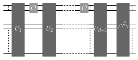
(a) A ${\rm QNC}_{d}$ circuit with access to oracle $\mathcal{O}$. Following [CCL20], in the oracle version of ${\rm QNC}_{d}$, we allow it to perform one extra single layered unitary to process the output.

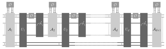
(b) A ${\rm QC}_{d}$ circuit with access to an oracle $\mathcal{O}$. There is no “extra” single layered unitary in this model.

(c) A ${\rm CQ}_{d}$ circuit with access to an oracle $\mathcal{O}$. Again, following [CCL20], we allow an extra single layer unitary to process the result of the last oracle call.

Figure 3: The same three circuit models, but with oracle access.

3 (Known) Technical Results I

The basic result we use, following [CCL20], is a simplified version of the so-called “one-way to hiding”, O2H lemma, introduced by [AHU18]. Informally, the lemma says the following: suppose there are two oracles $\mathcal{O}$ and $\mathcal{Q}$ which behave identically on all inputs except some subset $S$ of their input domain. Let $\mathcal{A}^{\mathcal{O}}$ and $\mathcal{A}^{\mathcal{Q}}$ be identical quantum algorithms, except for their oracle access, which is to $\mathcal{O}$ and $\mathcal{Q}$ respectively. Then, the probability that the result of $\mathcal{A}^{\mathcal{O}}$ and $\mathcal{A}^{\mathcal{Q}}$ will be distinct, is bounded by the probability of finding the set $S$. We suppress the details of the general finding procedure and only focus on the case of interest for us here.

3.1 Standard notions of distances

We quickly recall some notions of distances that appear here.

Definition 13.

Let $\rho,\rho^{\prime}$ be two mixed states. Then we define

• Fidelity: ${\rm F}(\rho,\rho^{\prime}):={\rm tr}(\sqrt{\sqrt{\rho}\rho^{\prime}\sqrt{\rho}})$

• Trace Distance: ${\rm TD}(\rho,\rho^{\prime}):=\frac{1}{2}{\rm tr}\left|\rho-\rho^{\prime}\right|$ and

• Bures Distance: ${\rm B}(\rho,\rho^{\prime}):=\sqrt{2-2F(\rho,\rho^{\prime})}$.

Fact 14.

For any string $s$, any two mixed states, $\rho$ and $\rho^{\prime}$, and any quantum algorithm $\mathcal{A}$, we have

$$\left|\Pr[s\leftarrow\mathcal{A}(\rho)]-\Pr[s\leftarrow\mathcal{A}(\rho^{\prime})]\right|\leq B(\rho,\rho^{\prime}).$$

3.2 The O2H lemma

Notation 15.

In the following, we treat $W$ as the workspace register for our algorithm which is left untouched by the Oracle and recall that $Q$ represents the query register and $R$ represents the response register.

In fact, we wish to allow parallel access to $\mathcal{Q}$ and we represent this by allowing queries to a tuple of inputs, $\boldsymbol{q}=(q_{1},q_{2}\dots q_{{\rm poly}(n)})$ simultaneously. We use boldface to represent such tuples. The query register in this case is denoted by $\boldsymbol{Q}$.

Definition 16 ($U^{\mathcal{L}\backslash S}$).

Suppose $U$ acts on $\boldsymbol{Q}RW$, $\mathcal{L}$ is an oracle that acts on $\boldsymbol{QR}$ and $S$ is a subset of the query domain of $\mathcal{L}$. We define

$$U^{\mathcal{L}\backslash S}\left|\psi\right\rangle_{\boldsymbol{QR}W}\left|0\right\rangle_{B}:=\mathcal{L}U_{S}U\left|\psi\right\rangle_{\boldsymbol{QR}W}\left|0\right\rangle_{B}$$

where $B$ is a qubit register, and $U_{S}$ flips qubit $B$ if any query is made inside the set $S$, i.e.

$$U_{S}\left|\boldsymbol{q}\right\rangle_{\boldsymbol{Q}}\left|b\right\rangle_{B}:=\begin{cases}U_{S}\left|\boldsymbol{q}\right\rangle_{\boldsymbol{Q}}\left|b\right\rangle_{B}&\text{if }\boldsymbol{q}\cap S=\emptyset\\ U_{S}\left|\boldsymbol{q}\right\rangle_{\boldsymbol{Q}}\left|b\oplus 1\right\rangle_{B}&\text{otherwise.}\end{cases}$$

Here we treat $\boldsymbol{q}$ as a set when we write $\boldsymbol{q}\cap S$.

For notational simplicity, in the following, we drop the boldface for the query and response registers as they do not play an active role in the discussion.

Definition 17 ($\Pr[{\rm find}:U^{\mathcal{L}\backslash S},\rho]$).

Let $U^{\mathcal{L}\backslash S}$ be as above and suppose $\rho\in{\rm D}(QRWB)$. We define

$$\Pr[{\rm find}:U^{\mathcal{L}\backslash S},\rho]:={\rm tr}[\mathbb{I}_{QRW}\otimes\left|1\right\rangle\left\langle 1\right|_{B}U^{\mathcal{L}\backslash S}\circ\rho].$$

This will depend on $\mathcal{L}$ and $S$. When $\mathcal{L}$ and $S$ are random variables, we additionally take expectation over them.

Remark 18.

Let $U^{\mathcal{L}\backslash S}$ be as in LABEL:Def:ULS and let $\left|\psi\right\rangle\in QRW$. Note that we can always write

$$\mathcal{L}U\left|\psi\right\rangle_{QRW}=\left|\phi_{0}\right\rangle_{QRW}+\left|\phi_{1}\right\rangle_{QRW}$$

where $\left|\phi_{0}\right\rangle$ and $\left|\phi_{1}\right\rangle$ contains queries outside $S$ and inside $S$ respectively, i.e. $\left\langle\phi_{0}|\phi_{1}\right\rangle=0$. Further, we can write

$$U^{\mathcal{L}\backslash S}\left|\psi\right\rangle_{QRW}\left|0\right\rangle_{B}=\left|\phi_{0}\right\rangle_{QRW}\left|0\right\rangle_{B}+\left|\phi_{1}\right\rangle_{QRW}\left|1\right\rangle_{B}.$$

Lemma 19 ([CCL20, AHU18] O2H).

Let

• $\mathcal{L}$ be an oracle which acts on $QR$ and $S$ be a subset of the query domain of $\mathcal{L}$,

• $\mathcal{G}$ be a shadow of $\mathcal{L}$ with respect to $S$, i.e. $\mathcal{G}$ and $\mathcal{L}$ behave identically for all queries outside $S$,

• further, suppose that within $S$, $\mathcal{G}$ responds with $\perp$ while (again within $S$), $\mathcal{L}$ does not respond with $\perp$. Finally, let $\Pi_{t}$ be a measurement in the computational basis, corresponding to the string $t$.

Then

$$\left|{\rm tr}[\Pi_{t}\mathcal{L}\circ U\circ\rho]-{\rm tr}[\Pi_{t}\mathcal{G}\circ U\circ\rho]\right| \leq B(\mathcal{L}\circ U\circ\rho,\mathcal{G}\circ U\circ\rho)$$

$$\leq\sqrt{2\Pr[\text{find }:U^{\mathcal{L}\backslash S},\rho]}.$$

If $\mathcal{L}$ and $S$ are random variables with a joint distribution, we take the expectation over them in the RHS (see LABEL:Def:prFind).

Proof.

We begin by assuming that $\mathcal{L}$ and $S$ are fixed (and so is $\mathcal{G}$). In that case, we can assume $\rho$ is pure. If not, we can purify it and absorb it in the work register. (The general case should follow from concavity). From LABEL:Rem:psiphi0phi1, we have

$$\left|\psi_{L}\right\rangle :=\mathcal{L}U\left|\psi\right\rangle_{Q^{\prime}}\overset{\ref{rem:psiphi0phi1}}{=}\left|\phi_{0}\right\rangle_{Q^{\prime}}+\left|\phi_{1}\right\rangle_{Q^{\prime}}.$$

$$\mathcal{L}U_{S}U\left|\psi\right\rangle_{Q^{\prime}}\left|0\right\rangle_{B} =\left|\phi_{0}\right\rangle_{Q^{\prime}}\left|0\right\rangle_{B}+\left|\phi_{1}\right\rangle_{Q^{\prime}}\left|1\right\rangle_{B}$$

where $Q^{\prime}$ is a shorthand for $QRW$. Similarly let

$$\left|\psi_{G}\right\rangle :=\mathcal{G}U\left|\psi\right\rangle_{Q^{\prime}}=\left|\phi_{0}\right\rangle_{Q^{\prime}}+\left|\phi_{1}^{\perp}\right\rangle_{Q^{\prime}}$$

where note that

$$\left\langle\phi_{1}|\phi_{1}^{\perp}\right\rangle_{QRW}=0$$ (6)

because $\left|\phi_{1}\right\rangle$ and $\left|\phi_{1}^{\perp}\right\rangle$ are the states where the queries were made on $S$, and on $S$ $\mathcal{G}$ responds with $\perp$ while $\mathcal{L}$ does not. Further, we analogously have

$$\mathcal{G}U_{S}U\left|\psi\right\rangle_{Q^{\prime}}\left|0\right\rangle_{B}=\left|\phi_{0}\right\rangle_{Q^{\prime}}\left|0\right\rangle_{B}+\left|\phi_{1}^{\perp}\right\rangle_{Q^{\prime}}\left|1\right\rangle_{B}.$$

We show that the difference between $\left|\psi_{L}\right\rangle$ and $\left|\psi_{G}\right\rangle$ is bounded by $P_{{\rm find}}(\mathcal{L},S):=\Pr[{\rm find}:U^{\mathcal{L}\backslash S},\rho]$, which in turn can be used to bound the quantity in the statement of the lemma.

$$\left\|\left|\psi_{L}\right\rangle-\left|\psi_{G}\right\rangle\right\|^{2} =\left\|\left|\phi_{1}\right\rangle-\left|\phi_{1}^{\perp}\right\rangle\right\|^{2}$$

$$\overset{\textup{(\ref{eq:phisPerp})}}{=}\left\|\left|\phi_{1}\right\rangle\right\|^{2}+\left\|\left|\phi_{1}^{\perp}\right\rangle\right\|^{2}$$

$$=2\left\|\left|\phi_{1}\right\rangle\right\|^{2} \because\left\|\left|\phi_{1}\right\rangle\right\|^{2}=\left\|\left|\phi_{1}^{\perp}\right\rangle\right\|^{2}=1-\left\|\left|\phi_{0}\right\rangle\right\|^{2}$$

$$=2P_{{\rm find}}(\mathcal{L},S).$$

If $\mathcal{L}$ and $S$ are random variables drawn from a (possibly) joint distribution $\Pr(\mathcal{L},S)$, the analysis can be generalised as follows. Let

$$\rho_{L} :=\sum_{\mathcal{L},S}\Pr(\mathcal{L},S)\left|\psi_{L}\right\rangle\left\langle\psi_{L}\right|$$

$$\rho_{G} :=\sum_{\mathcal{L},S}\Pr(\mathcal{L},S)\left|\psi_{G}\right\rangle\left\langle\psi_{G}\right|$$

where $\left|\psi_{G}\right\rangle$ is fixed by $\mathcal{L}$ and $S$ because $G$ itself is fixed once $\mathcal{L}$ and $S$ is fixed (by assumption). One can then use monotonicity of fidelity to obtain

$$F(\rho_{L},\rho_{G}) \geq\sum_{L,S}\Pr(\mathcal{L},S)F(\left|\psi_{L}\right\rangle,\left|\psi_{G}\right\rangle)$$

$$\geq 1-\frac{1}{2}.\sum_{L,S}\Pr(\mathcal{L},S)\left\|\left|\psi_{L}\right\rangle-\left|\psi_{G}\right\rangle\right\|^{2} \because 1-\frac{1}{2}F(\left|a\right\rangle,\left|b\right\rangle)\geq\left\|\left|a\right\rangle-\left|b\right\rangle\right\|^{2}$$

$$\geq 1-\cancel{\frac{1}{2}}\sum_{L,S}\Pr(\mathcal{L},S)\cancel{2}P_{{\rm find}}(\mathcal{L},S)$$

$$=1-P_{{\rm find}}$$

where $P_{{\rm find}}$ is the expectation of $P_{{\rm find}}(\mathcal{L},S)$ over $\mathcal{L}$ and $S$. It is known that the trace distance bounds the LHS of the Lemma and the trace distance itself is bounded by $\sqrt{2-2F}$.

∎

In the following, we resume the use of boldface for the query and response registers as they do play an active role in the discussion.

Lemma 20 ([CCL20, AHU18] Bounding $\Pr[{\rm find}:U^{\mathcal{L}\backslash S},\rho]$).

Suppose $S$ is a random variable and $\Pr[x\in S]\leq p$ for some $p$. Further, assume that $U$ and $\rho$ are uncorrelated to $S$. Then, (see LABEL:Def:ULS)

$$\Pr[{\rm find}:U^{\mathcal{L}\backslash S},\rho]\leq\bar{q}\cdot p$$

where $\bar{q}$ is the total number of queries $U$ makes to $\mathcal{L}$.

Proof.

Let us begin with the case where the oracle is applied only once, i.e. $\boldsymbol{Q}$ is a single query register $Q$. Since the $RW$ registers don’t play any significant role, we denote it by $L$. Let

$$U\left|\psi\right\rangle =\sum_{q,l}\psi(q,l)\left|q,l,0\right\rangle_{QLS}$$

$$\implies U_{S}U\left|\psi\right\rangle =\sum_{q\notin S}\left(\sum_{r,l}\psi(q,l)\left|q,l\right\rangle_{QL}\right)\left|0\right\rangle_{S}+\sum_{q\in S}\left(\sum_{r,l}\psi(q,l)\left|q,l\right\rangle_{QL}\right)\left|1\right\rangle_{S}.$$

Since $\mathcal{L}$ leaves registers $QS$ unchanged,

$${\rm tr}[\mathbb{I}_{QL}\otimes\left|1\right\rangle\left\langle 1\right|_{B}\left(\mathcal{L}\circ U_{S}\circ U\circ\left|\psi\right\rangle\left\langle\psi\right|\right)] ={\rm tr}[\mathbb{I}_{QL}\otimes\left|1\right\rangle\left\langle 1\right|_{B}\left(U_{S}\circ U\circ\left|\psi\right\rangle\left\langle\psi\right|\right)]$$

$$=\sum_{q}\psi^{2}(q)\chi_{S}(q)$$

where $\psi(q)=\sum_{l}\psi(q,l)$ and $\chi_{S}$ is the characteristic function for $S$, i.e.

$$\chi_{S}(q)=\begin{cases}1&q\in S\\ 0&q\notin S.\end{cases}$$

We are yet to average over the random variable $S$. Clearly, $\mathbb{E}(\chi_{S}(q))=\Pr[x\in S]\leq p$, yielding

$$\Pr[{\rm find}:U^{\mathcal{L}\backslash S},\rho]\leq p.$$

In the general case, everything goes through unchanged except the string $q$ is now a set of strings $\boldsymbol{q}$ and

$$\chi_{S}(\boldsymbol{q})=\begin{cases}1&\boldsymbol{q}\cap S\neq\emptyset\\ 0&\boldsymbol{q}\cap S=\emptyset.\end{cases}$$

Consequently, one evaluates $\mathbb{E}(\chi_{S}(\boldsymbol{q}))=\Pr[\boldsymbol{q}\cap S\neq\emptyset]\leq\left|\boldsymbol{q}\right|\cdot p=\bar{q}\cdot p$, by the union bound, yielding

$$\Pr[{\rm find}:U^{\mathcal{L}\backslash S},\rho]\leq\bar{q}\cdot p.$$

∎

We now generalise the statement slightly to facilitate the use of conditional random variables. These become useful for the proof of hardness for ${\rm QC}_{d}$ circuits.

Corollary 21.

Let $D$ be the query domain of $\mathcal{L}$. Suppose a set $S\subseteq D$, a quantum state $\rho$ and a unitary $U$ are drawn from a joint distribution (which may be correlated with $\mathcal{L}$). Let the set $T\subseteq D$ be another random variable (again, possibly arbitrarily correlated) and $F$ be the event that $S\cap T=\emptyset$. Define the random variables $\mathcal{N}:=\mathcal{L}|F$, $R:=S|F$, $\sigma:=\rho|F$ and $V:=U|F$ and assume that $R$, $\sigma$ and $V$ are uncorrelated. Suppose for all $x\in D$, $\Pr[x\in R]\leq p$ for some $p.$ Then, (see LABEL:Def:ULS)

$$\Pr[{\rm find}:V^{\mathcal{\mathcal{N}}\backslash R},\sigma]\leq\bar{q}\cdot p$$

where $\bar{q}$ is the total number of queries $V$ makes to $\mathcal{L}$.

4 $d$-Serial Simon’s Problem $\scriptscriptstyle\ll$ Main Result 1

In this section, we introduce the $d$-Serial Simon’s Problem. To get some familiarity, we first state the upper bounds—we see that it can be solved by a ${\rm QC}_{d+1}$ circuit and also by a ${\rm CQ}_{1}$ circuit. As for the lower bound, we begin by showing that no ${\rm QNC}_{d}$ circuit can solve the problem. We then extend this proof to show that no ${\rm QC}_{d}$ circuit can solve the problem either.

4.1 Oracles and Distributions — Simon’s and $c$-Serial

We begin with Simon’s problem. As will be the case for all problems we discuss, we consider both search and decision variants. The latter will usually take the form of distinguishing, say, a Simon’s oracle from a one-to-one oracle. We thus, first define the two oracles, and then use them to define both variants of the problem.

Definition 22 (Distribution for one-to-one functions).

Let $F:=\left\{f:\{0,1\}^{n}\to\{0,1\}^{n}|f\text{ is one-to-one}\right\}$ be the set of all one-to-one functions acting on $n$-bit strings, and let $\mathcal{O}_{F}:=\{\mathcal{O}_{f}:f\in F\}$ be the set of all oracles associated with these functions. Define the distribution over one-to-one functions, $\mathbb{F}_{R}(n)$, to be the uniform distribution over $F$ and the distribution for one-to-one function oracles, $\mathbb{O}_{{\rm R}}(n)$, to be the uniform distribution over $\mathcal{O}_{F}$.

Definition 23 (Distribution for Simon’s function).

Let

$$F:=\{(f,s)|f:\{0,1\}^{n}\to\{0,1\}^{n}\text{ is two-to-one and }f(x\oplus s)=f(x)\}$$

be the set of all Simon functions acting on $n$-bit strings and let $\mathcal{O}_{F}:=\{(\mathcal{O}_{f},s):(f,s)\in F\}$ be the set of all oracles associated with these functions. Define the distribution over Simon’s functions, $\mathbb{F}_{S}(n)$, to be the uniform distribution over $F$ and the distribution over Simon’s Oracles, $\mathbb{O}_{S}(n)$ to be the uniform distribution over $\mathcal{O}_{F}$.

Definition 24 (Simon’s Problem).

Fix an integer $n>0$ to denote the problem size. Let $\mathcal{R}\sim\mathbb{O}_{R}(n)$ be an oracle for a randomly chosen one-to-one function and $(\mathcal{S},s)\sim\mathbb{O}_{S}(n)$ be an oracle for a randomly chosen Simon’s function which has period $s$.

• Search version: Given $\mathcal{S}$, find $s$.

• Decision version: Given $\mathcal{O}\in_{R}\{\mathcal{R},\mathcal{S}\}$, i.e. one of the oracles with equal probability, determine which oracle was given.

While we focus on $d$-Serial Simon’s Problem, we define the problem more generally as a $d$-Serial Generic Oracle Problem with respect a “generic oracle problem”. To this end, we briefly formalise the latter.

Definition 25 (Generic Oracle Problem).

Let $(\mathcal{O},r)\sim\mathbb{O}(n)$ where $\mathbb{O}$ is some fixed distribution over oracles and the corresponding expected answers, and $n$ is the problem size. Let $\mathcal{R}\sim\cancel{\mathbb{O}}(n)$ where suppose that $\cancel{\mathbb{O}}(n)$ is the distribution over oracles against which the decision version is defined. The generic oracle problem is:

• Search version: Given $\mathcal{O},$ find $r$.

• Decision version: Given $\mathcal{Q}\in_{R}\{\mathcal{O},\mathcal{R}\}$, determine which oracle was given.

The $d$-Serial Generic Oracle problem is based on the following idea: there is a sequence of $d+1$ oracles (indexed $0,1\dots d$), of which the first $d$ encode a Simon’s problems. The zeroth oracle can be accessed directly. To access the first oracle, however, a secret key is needed. This secret is the period of the zeroth Simon’s function. The first oracle, once unlocked, behaves as a Simon’s oracle whose period unlocks the second oracle and so on. The Generic oracle is unlocked by the period of the $(d-1)$th Simon’s problem. The problem is to solve the “Generic Oracle problem” using the aforementioned $d+1$ oracles.

The intuition is quite simple. Consider the $d$-Serial Simon’s Oracle Problem, i.e. where the generic oracle problem is a Simon’s problem. Then, observe that, naïvely, a ${\rm QC}_{d}$ scheme would have to use all its $d$ depth to solve the $d$ Simon’s problems to access the last oracle and have no quantum depth left for solving the last Simon’s problem. However, with one more depth, i.e. with ${\rm QC}_{d+1}$, the problem can be solved. Further, note that a ${\rm CQ}_{1}$ scheme too can solve the problem. We will revisit these statements shortly but first, we formally define the problem.

Definition 26 ($c$-Serial Generic Oracle).

Suppose the Generic Oracle is sampled from the distributions $\mathbb{O}(n)$ and $\cancel{\mathbb{O}}(n)$ as in LABEL:Def:genericOracleProblem above where the oracles’ domain is assumed to be $\{0,1\}^{n}$. We define the $c$-Serial Generic Function distribution $\mathbb{F}_{{\rm Serial}}(c,n,\mathbb{O},\cancel{\mathbb{O}})$ and the $c$-Serial Generic Oracle distribution $\mathbb{O}_{{\rm Serial}}(c,n,\mathbb{O},\cancel{\mathbb{O}})$ by specifying its sampling procedure.

• Sampling step:

  • For $i\in\{0,1,2,\dots c-1\}$, $(f_{i},s_{i})\sim\mathbb{F}_{S}(n)$, i.e. sample $c$ Simon’s functions from $\mathbb{F}_{S}(n)$.

  • Sample $(\mathcal{O},r)\sim\mathbb{O}(n)$ and $\mathcal{R}\sim\cancel{\mathbb{O}}(n)$. For the search version, $\mathcal{Q}:=\mathcal{O}$ while for the decision version, $\mathcal{Q}\in_{R}\{\mathcal{O},\mathcal{R}\}$.

• Let $L_{f_{i}}:\{0,1\}^{n}\times\{0,1\}^{n}\to\{0,1\}^{n}\cup\{\perp\}$ for $i\in\{0,1,2,\dots c\}$ be defined as

  • $L_{f_{0}}(x,z)=f_{0}(x)$ when $i=0$ and

  • $L_{f_{i}}(x,z):=\begin{cases}f_{i}(x)&z=s_{i-1}\\ \perp&z\neq s_{i-1}\text{ when }i\in\{1,2,3\dots c-1\}.\end{cases}$

  • $L_{f_{c}}(x,z):=\begin{cases}\mathcal{Q}(x)&z=s_{c-1}\\ \perp&z\neq s_{c-1}.\end{cases}$

• Let $\mathcal{L}$ be the oracle associated with $(L_{f_{i}})_{i=0}^{c}$.

• Returns

  • $\mathbb{O}_{{\rm Serial}}$

    • Search: When $\mathbb{O}_{{\rm Serial}}(c,n,\mathbb{O})$ is sampled, consider the search version of the sampling step above and return $(\mathcal{L},r)$.

    • Decision: When $\mathbb{O}_{{\rm Serial}}(c,n,\mathbb{O},\cancel{\mathbb{O}})$ is sampled, consider the decision version of the sampling step above and return $(\mathcal{L},l)$ where $l=0$ if $\mathcal{Q}=\mathcal{O}$ and $l=1$ if $\mathcal{Q}=\mathcal{R}$.

  • $\mathbb{F}_{{\rm Serial}}$

    • When $\mathbb{F}_{{\rm Serial}}(c,n,\mathbb{O})$ is sampled, consider the search version of the sampling step above and return $(L_{f_{0}},s_{0},L_{f_{1}},s_{1}\dots L_{f_{c-1}},s_{c-1},L_{f_{c}},r)$, where recall that $(\mathcal{O},r)$ were sampled from $\mathbb{O}(n)$ and $\mathcal{Q}=\mathcal{O}$ (for the search version of the sampling step).

Definition 27 ($c$–Serial Generic Oracle Problem).

As before, we define two variants of the $c$-Serial Generic Oracle Problem:

• Search Variant: Let $(\mathcal{L},r)\sim\mathbb{O}_{{\rm Serial}}(c,n,\mathbb{O})$. Given $\mathcal{L}$, find $r$.

• Decision Variant: Let $(\mathcal{L},l)\sim\mathbb{O}_{{\rm Serial}}(c,n,\mathbb{O},\cancel{\mathbb{O}})$. Given $\mathcal{L}$, determine whether $l=0$ or $1$.

4.2 Depth upper bounds for $d$-Serial Simon’s Problem

One can use Simon’s algorithm for easily obtaining the following depth upper bounds for solving $d$-Serial Simon’s Problem. Note that while we only need $d+1$ queries to the oracle, we need to apply Hadamards before and after, for Simon’s algorithm to work. Thus, for ${\rm QC}$ circuits (which by definition allow only one layer of unitary before an oracle call, not after), we need depth $2d+2$ while for ${\rm CQ}$ circuits (which allow a layer of unitary before and after), we only need depth $1$.

Proposition 28.

The decision variant of the $d$-Serial Simon’s Problem is in ${\rm BQNC}_{2d+2}^{{\rm BPP}}$ and the search version can be solved using ${\rm QC}_{2d+2}$ circuits.

Proposition 29.

The decision variant of the $d$-Serial Simon’s Problem is in ${\rm BPP}^{{\rm BQNC}_{1}}$ and the search version can be solved using ${\rm CQ}_{1}$ circuits.

4.3 Depth lower bounds for $c$-Serial Simon’s problem

Following [CCL20], it would be useful to define “shadows” of oracles for establishing lower bounds. The idea is simple. Given an oracle and a subset $S$ of the query domain thereof, the shadow behaves exactly like the oracle when queried outside $S$ and outputs $\perp$ when queried inside $S$. Since there are multiple functions involved, for notational ease, we formalise this notion for a sequence of sets.

Definition 30 ($c$–Serial Generic Shadow Oracle).

Given

• $(L_{f_{i}},s_{i})_{i=0}^{c}$ from the sample space of $\mathbb{F}_{{\rm Serial}}(c,n,\mathbb{O})$, and

• a tuple of subsets $\bar{S}=(S_{1},S_{2},\dots S_{c})$ where $S_{i}\subseteq\{0,1\}^{n}\times\{0,1\}^{n}$,

let $\mathcal{L}$ be the oracle associated with $(L_{f_{i}})_{i=1}^{c}$. Then, the $c$-Serial Generic Shadow Oracle (or simply the shadow) $\mathcal{H}$ for the oracle $\mathcal{L}$ with respect to $\bar{S}$ is defined to be the oracle associated with $(L_{f_{0}},L_{f_{1}}^{\prime},L_{f_{2}}^{\prime}\dots L_{f_{c}}^{\prime})$ where

$$L^{\prime}_{f_{i}}:=\begin{cases}L_{f_{i}}(x,z)&(x,z)\in\{0,1\}^{2n}\backslash S_{i}\\ \perp&(x,z)\in S_{i}\end{cases}$$

for $i\in\{1,2\dots c\}$.

Remark 31.

For the moment, we exclusively consider the case where the “Generic Oracle” (drawn from $\mathbb{O}$) is also a Simon’s oracle (which are drawn from $\mathbb{O}_{S}$) and define the $c$-Serial Simon’s Oracle/Problem/Shadow Oracle implicitly.

As will become evident shortly, it would be useful to have shadows $\{\mathcal{M}_{i}\}_{i=1}^{d}$ such that $\mathcal{M}_{j}$ behaves like the $d$-Serial Simon’s oracle $\mathcal{L}$ at all sub-oracles from $0$ to $j-1$ but outputs $\perp$ for all subsequent sub-oracles (see LABEL:Fig:QNCd).

Algorithm 32 ($\bar{S}_{j}$ for ${\rm QNC}_{d}$ exclusion).

Input:

• $1\leq j\leq d$ and

• $(L_{f_{i}},s_{i})_{i=0}^{d}$ from the sample space of $\mathbb{F}_{{\rm Serial}}(c,n,\mathbb{O}_{S})$,

Output: $\bar{S}_{j}$, a tuple of $d$ subsets defined as

$$\bar{S}_{j}:=\begin{cases}(\emptyset,\emptyset,\dots\emptyset,E\times s_{j-1},E\times s_{j}\dots,E\times s_{d-1})&\text{for }j>1\\ (E\times s_{0},E\times s_{1}\dots,E\times s_{d-1})&\text{for }j=1\end{cases}$$

where $E=\{0,1\}^{n}$ and $\times$ is the Cartesian product.

4.3.1 Warm up — $d$-Serial Simon’s Problem is hard for ${\rm QNC}_{d}$

Theorem 33.

Let $(\mathcal{L},s)\sim\mathbb{O}_{{\rm Serial}}(d,n,\mathbb{O}_{S})$, i.e. let $\mathcal{L}$ be an oracle for a random $d$-Serial Simon’s Problem of size $n$ and period $s$. Let $\mathcal{A}^{\mathcal{L}}$ be any $d$ depth quantum circuit (see LABEL:Def:QNCd and LABEL:Rem:oracleVersionsQNC-CQ-QC) acting on $\mathcal{O}(n)$ qubits, with query access to $\mathcal{L}$. Then $\Pr[s\leftarrow\mathcal{A}^{\mathcal{L}}]\leq{\rm negl}(n)$, i.e. the probability that the algorithm finds the period is exponentially small.

Proof.

Suppose $(L_{f_{i}},s_{i})_{i=0}^{d}\sim\mathbb{F}_{{\rm Serial}}(d,n,\mathbb{O}_{S})$ (see LABEL:Def:cSerialSimonsOracle) and let $\mathcal{L}$ be the oracle associated with $(L_{f_{i}})_{i=0}^{d}$. For notational consistency, let $s=s_{d}$. Denote an arbitrary ${\rm QNC}_{d}^{\mathcal{L}}$ circuit, $\mathcal{A}^{\mathcal{L}}$, by

$$\mathcal{A}^{\mathcal{L}}:=\Pi\circ U_{d+1}\circ\mathcal{L}\circ U_{d}\dots\mathcal{L}\circ U_{2}\circ\mathcal{L}\circ U_{1}$$

and suppose $\Pi$ corresponds to the algorithm outputting the string $s$. For each $i\in\{1,\dots d\}$, construct the tuples $\bar{S}_{i}$ using LABEL:Alg:SforQNCd. Let $\mathcal{M}_{i}$ be the shadow of $\mathcal{L}$ with respect to $\bar{S}_{i}$ (see LABEL:Def:cSerialShadowOracle). Define

$$\mathcal{A}^{\mathcal{M}}:=\Pi\circ U_{d+1}\circ\mathcal{M}_{d}\circ U_{d}\dots\mathcal{M}_{2}\circ U_{2}\circ\mathcal{M}_{1}\circ U_{1}.$$

Note that $\Pr[s\leftarrow\mathcal{A}^{\mathcal{M}}]\leq\frac{1}{2^{n}}$ because no $\mathcal{M}_{i}$ contains any information about $f_{d}$, the last Simon’s function, whose period, $s$, is the required solution. Thus, no algorithm can do better than making a random guess. We now show that the output distributions of $\mathcal{A}^{\mathcal{L}}$ and $\mathcal{A}^{\mathcal{M}}$ cannot be noticeably different using the O2H lemma (see LABEL:Lem:O2H).

To apply the lemma, one can use the hybrid method as follows (we drop the $\circ$ symbol for brevity):

$$\left|\Pr[s\leftarrow\mathcal{A}^{\mathcal{L}}]-\Pr[s\leftarrow\mathcal{A}^{\mathcal{M}}]\right|$$

$$= \left|{\rm tr}[\Pi U_{d+1}\mathcal{L}U_{d}\dots\mathcal{L}U_{2}\mathcal{L}U_{1}\rho_{0}-\Pi U_{d+1}\mathcal{M}_{d}U_{d}\dots\mathcal{M}_{2}U_{2}\mathcal{M}_{1}U_{1}\rho_{0}]\right|$$

$$\leq \left|{\rm tr}[\Pi U_{d+1}\mathcal{L}U_{d}\dots\mathcal{L}U_{2}\underbrace{\mathcal{L}U_{1}\rho_{0}}-\Pi U_{d+1}\mathcal{L}U_{d}\dots\mathcal{L}U_{2}\underbrace{\mathcal{M}_{1}U_{1}\rho_{0}}]\right|+$$

$$\left|{\rm tr}[\Pi U_{d+1}\mathcal{L}U_{d}\dots U_{3}\underbrace{\mathcal{L}U_{2}\mathcal{M}_{1}U_{1}\rho_{0}}-\Pi U_{d+1}\mathcal{L}U_{d}\dots\mathcal{L}U_{3}\underbrace{\mathcal{M}_{2}U_{2}\mathcal{M}_{1}U_{1}\rho_{0}}]\right|+$$

$$\vdots$$

$$\left|{\rm tr}[\Pi U_{d+1}\underbrace{\mathcal{L}U_{d}\mathcal{M}_{d-1}U_{d-1}\dots U_{3}\mathcal{M}_{2}U_{2}\mathcal{M}_{1}U_{1}\rho_{0}}-\Pi U_{d+1}\underbrace{\mathcal{M}_{d}U_{d}\mathcal{M}_{d-1}\dots U_{3}\mathcal{M}_{2}U_{2}\mathcal{M}_{1}U_{1}\rho_{0}}]\right|$$

$$\leq {\rm B}(\mathcal{L}\circ U_{1}(\rho_{0}),\mathcal{M}_{1}\circ U_{1}(\rho_{0}))+$$

$${\rm B}(\mathcal{L}\circ U_{2}(\rho_{1}),\mathcal{M}_{2}\circ U_{2}(\rho_{1}))+$$

$$\vdots$$

$${\rm B}(\mathcal{L}\circ U_{d}(\rho_{d-1}),\mathcal{M}_{d}\circ U_{d}(\rho_{d-1}))$$

$$\leq \sum_{i=1}^{d}\sqrt{2\Pr[{\rm find}:U_{i}^{\mathcal{L}\backslash\bar{S}_{i}},\rho_{i-1}]}$$

where $\rho_{0}=\left|0\dots 0\right\rangle\left\langle 0\dots 0\right|$ and $\rho_{i}=\mathcal{M}_{i}\circ U_{i}\circ\dots\mathcal{M}_{1}\circ U_{1}(\rho_{0})$ for $i>0$. To bound the last expression, we apply LABEL:Lem:boundPfind. To apply the lemma, however, we must ensure that the subset of queries at which $\mathcal{L}$ and $\mathcal{M}_{i}$ differ, i.e. $\bar{S}_{i}=(\emptyset,\dots\emptyset,E\times s_{i-1},E\times s_{i}\dots E\times s_{d-1})$, (recall $E=\{0,1\}^{n}$) is uncorrelated to $U_{i}$ and $\rho_{i-1}$. Observe that $\rho_{i-1}$ is completely uncorrelated to $s_{i-1},s_{i},s_{i+1}\dots s_{d}$. At a high level, this is because $\rho_{i-1}$ can at most access $\mathcal{M}_{1},\dots\mathcal{M}_{i-1}$ and these in turn contain no information about $\bar{S}_{i}$. To see this, note that even though to define $\mathcal{M}_{1}$, we used $\bar{S}_{1}=(E\times s_{0},E\times s_{1}\dots,E\times s_{d-1})$, still $\mathcal{M}_{1}$ contains no information about $s_{1},\dots s_{d}$ because (other than the zeroth sub-oracle which can reveal $s_{0}$) it always outputs $\perp$. Similarly, $\mathcal{M}_{2}$ contains information about $s_{0},s_{1}$ but not about $s_{2},s_{3}\dots s_{d}$. Analogously for $\mathcal{M}_{3}$ and so on. Since the definition of $\rho_{i-1}$ only involves $\mathcal{M}_{1},\dots\mathcal{M}_{i-1}$, it contains no information about $s_{i-1},s_{i},s_{i+1}\dots s_{d}$. As for $U_{i}$, that is uncorrelated to all $s_{i}$s by construction.

Finally, to apply LABEL:Lem:boundPfind, we need to bound the probability that a fixed query, $x$, lands in the set $\bar{S}_{i}$. To this end, observe that $\Pr[x_{i}\in E\times s_{i}]=\frac{1}{2^{n}}$ when $s_{i}\in_{R}\{0,1\}^{n}$ and that the union bound readily bounds the desired probability, i.e. $\Pr[x\in\bar{S}_{i}]\leq d\cdot 2^{-n}$. Since $U$ acts on ${\rm poly}(n)$ many qubits, $q$ in the lemma can be set to ${\rm poly}(n)$. Thus, we can bound the last inequality by $d\cdot{\rm poly}(n)/2^{n}$. Using the triangle inequality, we get

$$\Pr[s\leftarrow\mathcal{A}^{\mathcal{L}}]\leq\frac{{\rm poly}(n)}{2^{n}}.$$

∎

4.3.2 $d$-Serial Simon’s Problem is hard for ${\rm QC}_{d}$

To prove our first main result—the same statement for ${\rm QC}_{d}$—we need to account for the possibility that the classical algorithm can make ${\rm poly}(n)$ many queries and process these before applying the next quantum layer. The high-level intuition is quite simple. We follow essentially the same strategy as in the ${\rm QNC}_{d}$ case, except that we successively condition the distribution over $\mathcal{L}$ to exclude the cases where the classical algorithm obtains a non-$\perp$ output.

To be slightly more precise, fix a particular $\mathcal{L}$. When the classical algorithm queries locations $T$, it could either get all $\perp$ responses or not get all $\perp$ responses (that is some responses may be non-$\perp$). We treat the latter case as though the classical algorithm solved the problem. For the former case, we conclude that the classical algorithm ruled out certain values of $s_{i}$s. We condition on this event and proceed similarly with the remaining analysis.

Since $\mathcal{L}$ is actually a random variable, notice that the probability that $\mathcal{L}$ responds with non-$\perp$ for a given $T$, is at most $\mathcal{O}({\rm poly}(n)\cdot 2^{-n})$. Thus, the probability that $\mathcal{L}$ responds with $\perp$ for all queries in $T$ is essentially $1$. Since we want an upper bound on the winning probability, we treat this conditional probability as $1$ and in the subsequent analysis, use $\mathcal{L}|T$ where $T$ is s.t. $\mathcal{L}(T)=\perp$. Since the shadows were defined using $\mathcal{L}$, they also get conditioned and the remaining analysis, essentially goes through unchanged. The only difference is that when $\Pr[{\rm find}:U^{\mathcal{L}\backslash S},\rho]$ is evaluated, because of the conditioning, the probabilities change by polynomial factors but these we have anyway been absorbing so the result remains unchanged.

Theorem 34.

Let $(\mathcal{L},s)\sim\mathbb{O}_{{\rm Serial}}(d,n,\mathbb{O}_{S})$, i.e. let $\mathcal{L}$ be an oracle for a random $d$-Serial Simon’s Problem of size $n$ and period $s$. Let $\mathcal{B}^{\mathcal{L}}$ be any ${\rm QC}_{d}$ circuit (see LABEL:Def:dQC and LABEL:Rem:oracleVersionsQNC-CQ-QC) with query access to $\mathcal{L}$. Then, $\Pr[s\leftarrow\mathcal{B}^{\mathcal{L}}]\leq{\rm negl}(n)$, i.e. the probability that the algorithm finds the period is exponentially small.

Proof.

The initial part of the proof is almost identical to that of the ${\rm QNC}_{d}$ case. Suppose $(L_{f_{i}},s_{i})_{i=0}^{d}\sim\mathbb{F}_{{\rm Serial}}(d,n,\mathbb{O}_{S})$ (see LABEL:Def:cSerialSimonsOracle) and let $\mathcal{L}$ be the oracle associated with $(L_{f_{i}})_{i=0}^{d}$. For notational consistency, let $s=s_{d}$. Recall that we denoted an arbitrary ${\rm QC}_{d}^{\mathcal{L}}$ circuit (see LABEL:Nota:CompositionNotation) with oracle access to $\mathcal{L}$,

$$\mathcal{B}^{\mathcal{L}}:=\Pi\circ\mathcal{A}_{c,d+1}^{\mathcal{L}}\circ\mathcal{B}_{d}^{\mathcal{L}}\circ\mathcal{B}_{d-1}^{\mathcal{L}}\dots\circ\mathcal{B}_{1}^{\mathcal{L}}\circ\rho_{0}$$

where $\mathcal{B}_{i}^{\mathcal{L}}:=\Pi_{i}\circ\mathcal{L}\circ U_{i}\circ\mathcal{A}_{c,i}^{\mathcal{L}}$, $\rho_{0}=\left|0\dots 0\right\rangle\left\langle 0\dots 0\right|$ and $\Pi$ corresponds to the algorithm outputting $s$. For each $i\in\{1,\dots d\}$, construct the tuples $\bar{S}_{i}$ using LABEL:Alg:SforQNCd. Let $\mathcal{M}_{i}$ be the shadow of $\mathcal{L}$ with respect to $\bar{S}_{i}$ (see LABEL:Def:cSerialShadowOracle). Define

$$\mathcal{B}^{\mathcal{M}}:=\Pi\circ\mathcal{A}_{c,d+1}^{\mathcal{L}}\circ\mathcal{B}_{d}^{\mathcal{M}}\circ\mathcal{B}_{d-1}^{\mathcal{M}}\dots\circ\mathcal{B}_{1}^{\mathcal{M}}.$$

where $\mathcal{B}_{i}^{\mathcal{M}}:=\Pi_{i}\circ\mathcal{M}_{i}\circ U_{i}\circ\mathcal{A}_{c,i}^{\mathcal{L}}$. We have

$$\left|\Pr[s\leftarrow\mathcal{B}^{\mathcal{L}}]-\Pr[s\leftarrow\mathcal{B}^{\mathcal{M}}]\right|$$

$$= \left|{\rm tr}[\Pi\mathcal{A}_{c,d+1}^{\mathcal{L}}\mathcal{B}_{d}^{\mathcal{L}}\mathcal{B}_{d-1}^{\mathcal{L}}\dots\mathcal{B}_{1}^{\mathcal{L}}\rho_{0}]-{\rm tr}[\Pi\mathcal{A}_{c,d+1}^{\mathcal{L}}\mathcal{B}_{d}^{\mathcal{M}}\mathcal{B}_{d-1}^{\mathcal{M}}\dots\mathcal{B}_{1}^{\mathcal{M}}\rho_{0}]\right| \text{we dropped }\circ\text{ for brevity}$$

$$\leq {\rm B}(\mathcal{B}_{1}^{\mathcal{L}}(\rho_{0}),\mathcal{B}_{1}^{\mathcal{M}}(\rho_{0}))+$$

$${\rm B}(\mathcal{B}_{2}^{\mathcal{L}}(\rho_{1}),\mathcal{B}_{2}^{\mathcal{M}}(\rho_{1}))+$$

$$\vdots$$

$${\rm B}(\mathcal{B}_{d}^{\mathcal{L}}(\rho_{d-1}),\mathcal{B}_{2}^{\mathcal{M}}(\rho_{d-1}))$$

$$= \sum_{i=1}^{d}\sqrt{2\Pr[{\rm find}:U_{i}^{\mathcal{L}\backslash\bar{S}_{i}},\mathcal{A}_{c,i}^{\mathcal{L}}\circ\rho_{i-1}]}.$$

where for $i\in\{1,2\dots d-1\}$, $\rho_{i}:=\mathcal{B}_{i}^{\mathcal{M}}\circ\dots\circ\mathcal{B}_{1}^{\mathcal{M}}\circ\rho_{0}$.

So far, everything was essentially the same as in the ${\rm QNC}_{d}$ case. The difference arises because of the classical algorithm. We begin with the first term, $\Pr[{\rm find}:U_{1}^{\mathcal{L}\backslash\bar{S}_{1}},\mathcal{A}_{c,1}^{\mathcal{L}}\circ\rho_{0}]$ and denote by $\bar{T}_{1}=(T_{1,1},T_{1,2}\dots T_{1,d})$ the tuple of subsets queried by $\mathcal{A}_{c,1}$. There are two possibilities: either all queries in $\bar{T}_{1}$ result in $\perp$ or at least one query yields a non-$\perp$ result. We treat the second event as though the algorithm was able to “find” the solution. Denote the first event by $F_{1}:=\bar{S}_{1}\cap\bar{T}_{1}=\emptyset$ and the second event as $\neg F_{1}:=\bar{S}_{1}\cap\bar{T}_{1}\neq\emptyset$ where the intersection is component-wise. Note that the random variable of interest here is $\mathcal{L}$ and those derived using it, i.e. $\mathcal{M}_{i}s$ and $\bar{S}_{i}$s. While the notation is cumbersome, we can use $\Pr[E]=\Pr[E|F]\Pr[F]+\Pr[E|\neg F]\Pr[\neg F]\leq\Pr[E|F]+\Pr[\neg F]$, to write

$$\Pr[{\rm find}:U_{1}^{\mathcal{L}\backslash\bar{S}_{1}},\mathcal{A}_{c,1}^{\mathcal{L}}\circ\rho_{0}]\leq\Pr[{\rm find}:V_{1}^{\mathcal{N}_{1}\backslash\bar{R}_{1}},\sigma_{0}]+\Pr[\neg F_{1}]$$ (7)

where $\sigma_{0}:=\mathcal{A}_{c,1}^{\mathcal{L}}\circ\rho_{0}|F_{1}$, $\bar{R}_{1}:=\bar{S}_{1}|F_{1}$, $\mathcal{N}_{1}=\mathcal{L}|F_{1}$ and $V_{1}:=U_{1}|F_{1}$. First, it is clear that $\Pr[\neg F_{1}]\leq\mathcal{O}({\rm poly}(n)2^{-n})$ by the union bound as $\Pr[x\in E\times s_{i}]\leq 2^{-n}$ for all $i\in\{1,2\dots d\}$. Second, $\mathcal{N}_{1}$ is uncorrelated to $\sigma_{0}$, and $V_{1}$ because we have restricted the sample space to the cases where the correlation is absent by conditioning on $F_{1}$ (i.e. $\bar{T}_{1}$ has been effectively removed from this part of the analysis). In more detail, the algorithm $\mathcal{A}_{c,1}$ (conditioned on event $F_{1}$), ruled out a polynomial number of locations where the various $E\times s_{i}$s are not. In the remaining query domain, $E\times s_{i}$s are not restricted, i.e. $\mathcal{N}_{1}$ is uncorrelated with $\sigma_{0}$. This also means that $\bar{R}_{1}$ is uncorrelated with $\sigma_{0}$. Finally, note that $\Pr[x\in\bar{R}_{1}]\leq\mathcal{O}\left(\frac{1}{2^{n}-{\rm poly}(n)}\right)\leq\mathcal{O}({\rm poly}(n)2^{-n})$. We can therefore apply LABEL:Cor:Conditionals to obtain the bound the first term in LABEL:Eq:QCd_analysis_first with $\mathcal{O}({\rm poly}(n)2^{-n})$. This yields

$$\Pr[{\rm find}:U_{1}^{\mathcal{L}\backslash\bar{S}_{1}},\mathcal{A}_{c,1}^{\mathcal{L}}\circ\rho_{0}]\leq\mathcal{O}({\rm poly}(n)2^{-n})$$

We now apply this reasoning to the second term,

$$\Pr[{\rm find}:U_{2}^{\mathcal{L}\backslash\bar{S}_{2}},\mathcal{A}_{c,2}^{\mathcal{L}}\circ\underbrace{\Pi_{1}\circ\mathcal{M}_{1}\circ U_{1}\circ\mathcal{A}_{c,1}^{\mathcal{L}}\circ\rho_{0}}_{\rho_{1}}].$$

It is clear, that $\rho_{1}$ can contain information about $s_{0}$ (as it has access to $\mathcal{M}_{1}$) and therefore $\bar{S}_{2}$ was chosen so that $\mathcal{M}_{2}$ and $\mathcal{L}$ behave identically when their zeroth sub-oracle is queried (whose “access requires $s_{0}$ and secret is $s_{1}$”, see LABEL:Fig:ShadowsQNCd). Additionally, $\mathcal{A}_{c,1}^{\mathcal{L}}$ may have partially learnt something about the remaining $s_{i}$s as well and this would prevent us from applying LABEL:Lem:boundPfind. We condition as in the case above to obtain

$$\Pr[{\rm find}:U_{2}^{\mathcal{L}\backslash\bar{S}_{2}},\mathcal{A}_{c,2}^{\mathcal{L}}\circ\rho_{1}]\leq\Pr[{\rm find}:V_{2}^{\mathcal{N}_{2}\backslash\bar{R}_{2}},\mathcal{A}_{c,2}^{\mathcal{N}_{2}}\circ\sigma_{1}]+\Pr[\neg F_{1}]$$ (8)

where $\sigma_{1}:=\rho_{1}|F_{1}$, $\mathcal{N}_{2}:=\mathcal{L}|F_{1}$, $V_{2}:=U_{2}|F_{1}$ and $\bar{R}_{2}:=\bar{S}_{2}|F_{1}$. The first term restricts the sample space (of $\mathcal{L}$) such that $\sigma_{1}$ is uncorrelated with $\bar{R}_{2}$. We are therefore essentially in the same situation as the starting point of the case above (see LABEL:Eq:QCd_analysis_first). Let $\bar{T}_{2}$ be the set where $\mathcal{A}_{c,2}^{\mathcal{N}_{2}}$ queries and define the event $F_{2}:=\bar{R}_{2}\cap\bar{T}_{2}=\emptyset$. Conditioning on $F_{2}$, we can bound the first term as

$$\Pr[{\rm find}:V_{2}^{\mathcal{N}_{2}\backslash\bar{R}_{2}},\mathcal{A}_{c,2}^{\mathcal{N}_{2}}\circ\sigma_{1}]\leq\Pr[{\rm find}:W_{2}^{\mathcal{O}_{2}\backslash\bar{Q}_{2}},\tau_{2}]+\Pr[\neg F_{2}]$$ (9)

where $\tau_{1}:=\mathcal{A}_{c,2}^{\mathcal{N}_{2}}\circ\sigma_{1}|F_{2}$, $\mathcal{O}_{2}:=\mathcal{N}_{2}|F_{1}$, $W_{2}:=V_{2}|F_{2}$ and $\bar{Q}_{2}:=\bar{R}_{2}|F_{2}$. Now, $\bar{Q}_{2}$ is uncorrelated to $\tau_{1}$ because we restricted to the part of the sample space where the effect $\mathcal{A}_{c,2}^{\mathcal{N}_{2}}$ has been accounted for. To see this, observe that after the conditioning, the reasoning is analogous to why $\rho_{1}$ is uncorrelated to $\bar{S}_{2}$. We can now apply LABEL:Cor:Conditionals with $\Pr[x\in\bar{Q}_{2}]\leq\mathcal{O}({\rm poly}(n)2^{-n})$, $\Pr[\neg F_{2}]\leq\mathcal{O}({\rm poly}(n)2^{-n})$ in LABEL:Eq:QCd_2_2 and combine it with LABEL:Eq:QCd_2_1 to obtain

$$\Pr[{\rm find}:U_{2}^{\mathcal{L}\backslash\bar{S}_{2}},\mathcal{A}_{c,2}^{\mathcal{L}}\circ\rho_{1}]\leq\mathcal{O}({\rm poly}(n)2^{-n}).$$

Proceeding similarly, one obtains the final bound. ∎

5 Warm-up — $d$-Shuffled Simon’s Problem ($d$-SS)

In the previous section, we established the first main result of this work—for each $d$, we saw that $d$-Serial Simon’s problem is easy for a ${\rm CQ}_{1}$ circuit but hard for ${\rm QC}_{d}$. Our second main goal is to show that for each $d$, there is a problem which is easy for ${\rm QC}_{c}$ (for some constant $c>0$, wrt $d$ and $n$) but hard for ${\rm CQ}_{d}$. However, showing depth lower bounds for ${\rm CQ}_{d}$ circuits can get quite involved. We, therefore, first re-derive a result due to [CCL20]—for each $d$, there is a problem which is easy for ${\rm CQ}_{2d+1}$ but hard for ${\rm CQ}_{d}$. While we use essentially the same problem (more on this momentarily), our proof is different and simpler. We build upon these techniques for proving our second main result in LABEL:Sec:ShuffledCollisionsToSimons.

The problem we consider in this section is called $d$-Shuffled Simon’s Problem which is essentially the same as the $d$-Shuffling Simon’s Problem introduced by [CCL20]. The difference arises in the way we construct the Shuffler and consequently in its analysis.

5.1 Oracles and Distributions

5.1.1 $d$-Shuffler

Notation 35.

We identify binary strings with their associated integer values implicitly. E.g. $f:\{0,1\}^{2n}\to\{0,1\}^{2n}$ then we may use $f(2^{n}-1)$ to denote $f(00\dots 0\underbrace{11\dots 1}_{n\text{ many}})$.

We begin with defining a $d$-Shuffler for a function $f$. We give two equivalent definitions of a $d$-Shuffler. The first is more intuitive but the second is easier to analyse.

A $d$-Shuffler for $f:\{0,1\}^{n}\to\{0,1\}^{n}$ is simply a sequence of $d$ permutations $f_{0},f_{1}\dots f_{d-1}$ on a larger space, which uses $2n$ length strings and a function $f_{d}$ such that $f_{d}\circ f_{d-1}\dots f_{0}(x)=f(x)$ for all $x$ in the domain of $f$ and for all points untouched by these “paths” originating from the domain of $x$, the permutations are modified to output $\perp$.

This definition makes counting arguments slightly convoluted. We therefore observe that a sequence of permutations may equivalently be specified by a sequence of tuples. For instance two permutations over four elements may be expressed as $[0,1,2,3]^{T}\mapsto[1,3,0,2]^{T}\mapsto[2,0,3,1]^{T}$ but the advantage here is that restricting the permutation to a subset (as we did above by defining the permutations to be $\perp$ outside the “paths”), corresponds to simply dropping some elements from the tuple: $[0,1]^{T}\mapsto[1,3]^{T}\mapsto[2,0]^{T}$. See LABEL:Fig:Sequence-of-tuples.

Figure 4: Sequence of tuples instead of restricted permutation functions.

Definition 36 (Uniform $d$-Shuffler for $f$).

A uniform $d$-Shuffler for a function $f:\{0,1\}^{n}\to\{0,1\}^{n}$ is a sequence of random functions $(f_{0},f_{1},\dots f_{d})$, where $f_{0},\dots f_{d}:\{0,1\}^{2n}\cup\{\perp\}\to\{0,1\}^{2n}\cup\{\perp\}$ sampled from a distribution $\mathbb{F}_{{\rm shuff}}(d,n,f)$ (to be defined) such that $f_{d}\circ f_{d-1}\dots\circ f_{0}(x)=f(x)$ for all $x\in Z\times\{0,1\}^{n}$ where $Z:=\{(0,\dots 0)\}$ (containing an $n$-bit zero string). Let $\mathcal{L}$ be the oracle associated with $(f_{i})_{i=0}^{d}$ and define $\mathbb{O}_{{\rm shuff}}(d,n,f)$ to be the corresponding distribution.

The sampling process is defined in two equivalent ways.
First definition:

• Sample $f^{\prime}_{0},\dots f^{\prime}_{d-1}:\{0,1\}^{2n}\to\{0,1\}^{2n}$ from a uniform distribution of permutation functions acting on strings of length $2n$.

• Define $f_{d}$ to be such that $f_{d}\circ f^{\prime}_{d-1}\circ\dots\circ f^{\prime}_{0}(x)=f(x)$ for all $x\in Z\times\{0,1\}^{n}$ and $f_{d}\circ f^{\prime}_{d-1}\circ\dots f^{\prime}_{0}(x)=\perp$ otherwise.

• For each $i\in\{0,1\dots d-1\}$,

  • define $X_{i+1}:=f_{i}^{\prime}\circ\dots f_{0}^{\prime}(X_{0})$ where $X_{0}=Z\times\{0,1\}^{n}$ and

  • define

    $$f_{i}(x):=\begin{cases}f^{\prime}_{i}(x)&\forall x\in X_{i-1}\\ \perp&\forall x\notin X_{i-1}.\end{cases}$$

Second equivalent definition:

• Let $t_{0},t_{1}\dots t_{d-1}$ each be a tuple $(x_{1},x_{2}\dots x_{N})$ of size $N:=2^{n}$, sampled uniformly from the collection of all size $N$ tuples containing distinct elements $x_{i}\in\{0,1\}^{2n}$. Let $t_{-1}:=(0,1,\dots N)$ and $t_{d}:=(f(0),f(1)\dots f(N-1))$ (see LABEL:Nota:IntegerString).

• $f_{0},\dots f_{d}$ — For each $i\in\{0,\dots,d-1\}$, define $f_{i}$ as follows.

  • If $x\notin t_{i-1}$, then define $f_{i}(x)=\perp$.

  • Otherwise, suppose $x$ is the $j$th element in $t_{i-1}$ and $y$ is the $j$th element in $t_{i}$. Then, define $f_{i}(x)=y$.

Given the second definition, a $d$-Shuffler may equivalently be defined as a sequence $(t_{0},\dots t_{d-1},t_{d})$ of tuples sampled as described above. We overload the notation and let $\mathbb{F}_{{\rm shuff}}(d,n,f)$ return $(t_{i})_{i=0}^{d}$ and similarly let $\mathbb{O}_{{\rm shuff}}(d,n,f)$ return the oracle associated with $(t_{i})_{i=0}^{d}$.

Finally, if $f$ is omitted when $\mathbb{F}_{{\rm shuff}}$ or $\mathbb{O}_{{\rm shuff}}$ are invoked, then it is assumed that $f\sim\mathbb{F}_{R}(n)$.

Notation 37.

In this section, we drop the word “uniform” for conciseness.

5.1.2 The $d$-SS Problem

Definition 38 ($d$-Shuffled Simon’s Distribution and Oracle).

We define the $d$-Shuffled Simon’s Function distribution, $\mathbb{F}_{{\rm SS}}(d,n)$ and the corresponding $d$-Shuffled Simon’s Oracle distribution $\mathbb{O}_{{\rm SS}}(d,n)$ by specifying its sampling procedure.

• Sample a random Simon’s function $(f,s)\sim\mathbb{F}_{{\rm S}}(n)$ (see LABEL:Def:SimonsFunctionDistr).

• Sample a $d$-Shuffler $(f_{i})_{i=0}^{d}\sim\mathbb{F}_{{\rm Shuff}}(d,n,f)$ where $f_{i}$ are functions (see LABEL:Def:dShuffler).

Return $((f_{i})_{i=0}^{d},s)$ when $\mathbb{F}_{{\rm SS}}(d,n)$ is sampled and $(\mathcal{F},s)$ when $\mathbb{O}_{{\rm SS}}(d,n)$ is sampled where $\mathcal{F}$ is the oracle associated with $(f_{i})_{i=0}^{d}$.

Definition 39 ($d$-Shuffled Simon’s Problem).

Let $(\mathcal{F},s)\sim\mathbb{O}_{{\rm SS}}(d,n)$ (see LABEL:Def:dShuffledSimonsDistr) be sampled from the $d$-Shuffled Simon’s Oracle distribution and $\mathcal{Q}\sim\mathbb{O}_{{\rm Shuff}}(d,n)$ be a random $d$-Shuffler (see LABEL:Def:dShuffler). The $d$-Shuffled Simon’s Problem is,

• Search version: Given $\mathcal{F}$, find $s$.

• Decision version: Given either $\mathcal{F}$ or $\mathcal{Q}$ with equal probability, output $1$ if $\mathcal{F}$ was given and $0$ otherwise.

5.2 Shadow Boilerplate

For the analysis, we need to consider shadow oracles associated with the $d$-Shuffled Simon’s Oracle. The definition is somewhat redundant—it is the direct analogue of LABEL:Def:cSerialShadowOracle. See LABEL:Fig:Shadows-for-d-ShuffledSimons.

Definition 40 ($d$-Shuffled Simon’s Shadow Oracle).

Given

• $((f_{i})_{i=0}^{d},s)$ from the sample space of $\mathbb{F}_{{\rm SS}}(d,n)$ and

• a tuple of subsets $\bar{S}=(S_{1},S_{2}\dots S_{d})$ where each $S_{i}\subseteq\{0,1\}^{2n}$,

let $\mathcal{F}$ be the oracle associated with $(f_{i})_{i=0}^{d}$. Then, the $d$-Shuffled Simon’s Shadow Oracle (or simply the shadow) $\mathcal{G}$for the oracle $\mathcal{F}$ with respect to $\bar{S}$ is defined to be the oracle associated with $(f_{0},f_{1}^{\prime}\dots f_{d}^{\prime})$ where

$$f^{\prime}_{i}:=\begin{cases}f_{i}(x)&x\in\{0,1\}^{2n}\backslash S_{i}\\ \perp&x\in S_{i}.\end{cases}$$

for all $i\in\{1,2\dots d\}$.

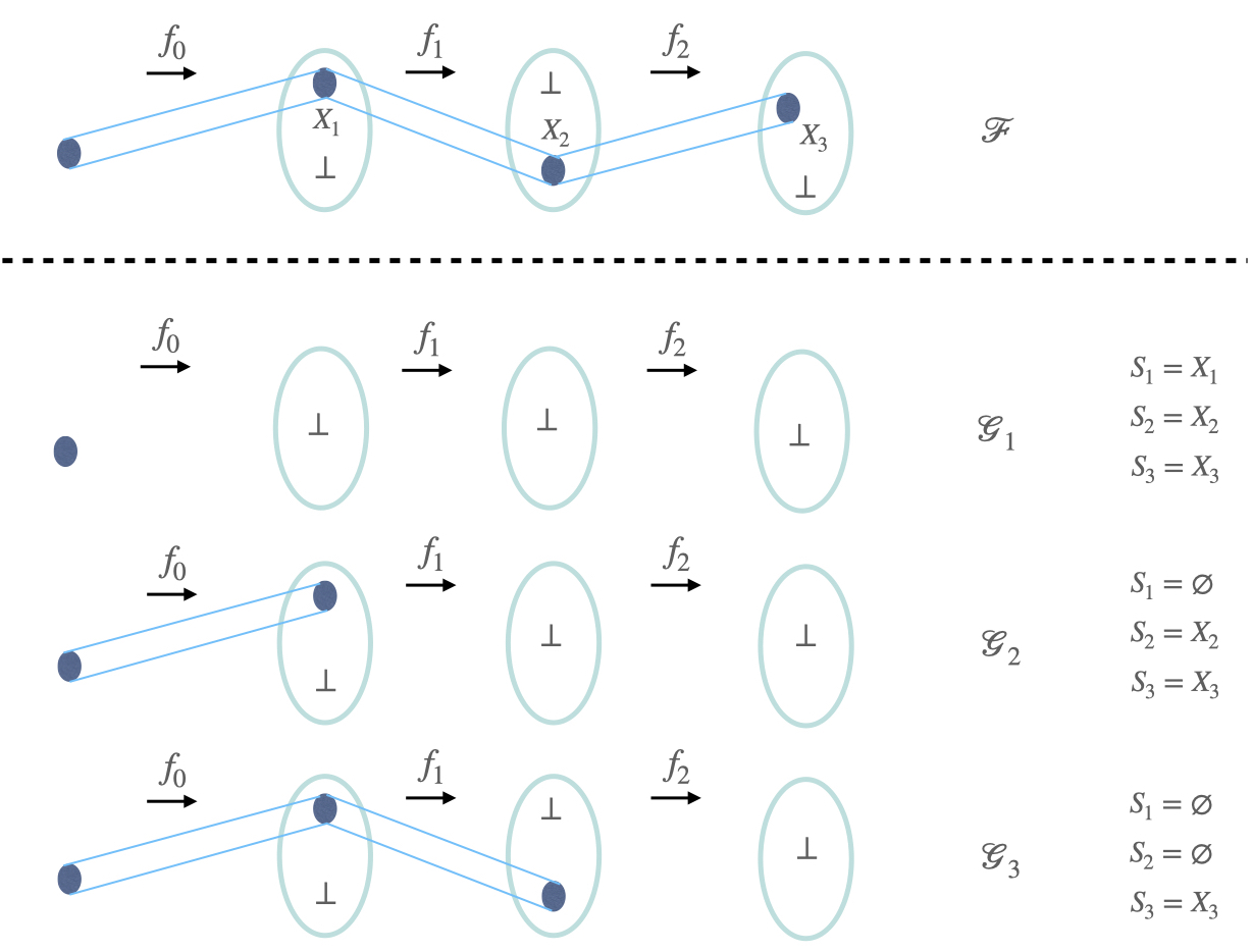
Figure 5: Shadows for $d$-Shuffled Simon’s Oracle. Ignore the arrows below the function labels $f_{0},\dots f_{2}$ at first. Suppose $d=3$. Consider the row for $\mathcal{F}$. As before, the ovals represent the query domains of functions $f_{0},f_{1},f_{2}$ and $f_{3}$. Similarly for the shadows $\mathcal{G}_{1},\dots\mathcal{G}_{3}$. The shaded regions denote a non-$\perp$ response. Let $\bar{S}_{i}$ be the query domain at which $\mathcal{F}$ and $\mathcal{G}_{i}$ differ. The construction, as before, ensures that $\mathcal{G}_{1}\dots\mathcal{G}_{i-1}$ do not contain any information about $\bar{S}_{i}$.

The analysis here is a straightforward adaptation of the ${\rm QNC}_{d}$ analysis for $d$-Serial Simon’s. Thus, we use the analogue of LABEL:Alg:SforQNCd_using_dSS. The only difference is in the numbering convention. The domain of the $i$th oracle was determined by $s_{i-1}$ in LABEL:Alg:SforQNCd_using_dSS while here, the domain of the $i$th oracle is determined by $X_{i}$.

Algorithm 41 ($\bar{S}_{j}$ for ${\rm QNC}_{d}$ exclusion using $d$-SS).

Input:

• $1\leq j\leq d$ and

• $((f_{i})_{i=0}^{d},s)$ from the sample space of $\mathbb{F}_{{\rm SS}}(d,n)$.

Output: $\bar{S}_{j}$, a tuple of $d$ subsets, defined as

$$\bar{S}_{j}:=\begin{cases}(\emptyset,\dots\emptyset,X_{j},\dots X_{d})&j>1\\ (X_{1},\dots X_{d})&j=1\end{cases}$$

where for each $i\in\{1,\dots d\}$, $X_{i}=f_{i-1}(X_{i-1})$ with $X_{0}=\{0,1\}^{n}$.

Proposition 42.

For all $2\leq i\leq d$, let $\mathcal{G}_{1}\dots\mathcal{G}_{i-1}$ denote the shadows of $(\mathcal{F},s)\in\mathbb{O}_{{\rm SS}}(d,n)$ (see LABEL:Def:d-ShuffledSimonShadow) with respect to $\bar{S}_{1}\dots\bar{S}_{i-1}$ (constructed using LABEL:Alg:SforQNCd_using_dSS with the index and $\mathcal{F}$ as inputs). Then, $\mathcal{G}_{1}\dots\mathcal{G}_{i-1}$ contain no information about $\bar{S}_{i}$.

Proof.

To see this, note that even though to define $\mathcal{G}_{1}$, we used $\bar{S}_{1}=(X_{1},X_{2}\dots X_{d}),$ still $\mathcal{G}_{1}$ contains no information about $X_{2},\dots X_{d}$ (and so no information about $\bar{S}_{2}$ either) because it always outputs $\perp$ (except for the zeroth oracle which can reveal $X_{1}$). Similarly, $\mathcal{G}_{2}$ contains information about $X_{1},X_{2}$ but not about $X_{3}\dots X_{d}$ (thus $\bar{S}_{3}$). Analogously for $\mathcal{G}_{3}$ and so on. ∎

Proposition 43.

Let $\bar{S}_{i}$ be the output of LABEL:Alg:SforQNCd_using_dSS with $i$ and $(\mathcal{F},s)$ as inputs where $(\mathcal{F},s)\sim\mathbb{O}_{{\rm SS}}(d,n)$ (see LABEL:Def:d-ShuffledSimonShadow). Let $x$ be some fixed query (in the query domain of $\mathcal{F}$). Then, $\Pr[x\in\bar{S}_{i}]\leq\mathcal{O}(d\cdot 2^{-n})$.

Proof.

For any fixed $x_{i}\in\{0,1\}^{2n}$, $\Pr[x_{i}\in X_{i}]=\frac{1}{2^{n}}$ (see LABEL:Rem:Pr_x_in_X_or_t using $N=2^{n}$ and $M=2^{2n}$). The union bound, then, readily bounds the desired probability. ∎

5.3 Depth Lower bounds for $d$-Shuffled Simon’s Problem ($d$-SS)

Again, as in the analysis for $d$-Serial Simon’s problem, we begin with briefly demonstrating the depth lower bound for ${\rm QNC}_{d}$ (with classical post-processing) and then generalise it to ${\rm CQ}_{d}$.

5.3.1 $d$-Shuffled Simon’s Problem is hard for ${\rm QNC}_{d}$

Theorem 44 ($d$-SS is hard for ${\rm QNC}_{d}$).

Let $(\mathcal{F},s)\sim\mathbb{O}_{{\rm SS}}(d,n)$, i.e. let $\mathcal{F}$be an oracle for a random $d$-Shuffled Simon’s problem of size n and period $s$. Let $\mathcal{A}^{\mathcal{F}}$ be any $d$ depth quantum circuit (see LABEL:Def:QNCd and LABEL:Rem:oracleVersionsQNC-CQ-QC) acting on $\mathcal{O}(n)$ qubits, with query access to $\mathcal{F}$. Then $\Pr[s\leftarrow\mathcal{A}^{\mathcal{F}}]\leq{\rm negl}(n)$, i.e. the probability that the algorithm finds the period is exponentially small.

This follows from the proof of LABEL:Thm:QNCd-dSerialSimons with no essential change. The main difference is in the details of how the shadow is constructed—earlier it was comprised of $E\times s_{i}$s, now $X_{i}$s comprise it. However, that doesn’t change the relevant properties (see LABEL:Prop:Shadow_dSS and LABEL:Prop:x_in_S_dSS_shadow) for the main argument (which is given explicitly in LABEL:Subsec:Hardness-of-dSS-for-QNCd for completeness).

We expect the ${\rm QNC}_{d}$ hardness of $d$-SS to readily generalise to hardness for ${\rm QC}_{d}$ (following the $d$-Serial Simon’s hardness proof) but we do not prove it here.

5.3.2 $d$-Shuffled Simon’s Problem is hard for ${\rm CQ}_{d}$ — idea

The generalisation to ${\rm CQ}_{d}$ takes some work. We first describe the basic idea behind our approach and then formalise these. These draw from the insights of [CCL20] but differ substantially in their implementation. Let $((f_{i})_{i=0}^{d},s)\sim\mathbb{F}_{{\rm SS}}(d,n)$. For our discussion, we require three key concepts.

1. The first, already introduced in the proof of LABEL:Thm:QCd_hardness_dSerialSimons, was the notion of conditioning the oracle distribution (and the quantities that depend on it) based on a “transcript” as the algorithm proceeds and analysing the conditioned cases. In the proof of LABEL:Thm:QCd_hardness_dSerialSimons, the locations queried by the classical algorithm constituted this transcript but it could, and as we shall see it will, more generally contain other correlated variables.

2. The second, is the notion of an almost uniform $d$-Shuffler. Neglect, for the moment, the last function $f_{d}$ which is used to define the $d$-Shuffler, $(f_{i})_{i=0}^{d}$. Then, informally, suppose that an algorithm (which can even be computationally unbounded) is given access to a uniform $d$-Shuffler and it produces a ${\rm poly}(n)$ sized advice (a string that is correlated with the Shuffler). One can show that for advice strings which appear with non-vanishing probability, the $d$-Shuffler conditioned on the advice string, continues to stay almost uniform.

3. The third, is basically the bootstrapping of the proof of LABEL:Thm:d-SS-is-hard-for-QNC-d, by letting it now play the role of the algorithm mentioned above. This ties the loose end left above, the question of correlation with $f_{d}$. A generic ${\rm QNC}_{d}$ circuit may reveal some information about $(f_{0},\dots f_{d-1})$ and $f_{d}$ in the poly-length string it outputs, however, the proof of LABEL:Thm:d-SS-is-hard-for-QNC-d guarantees that the behaviour of this algorithm cannot be very different from one which has no access to $f_{d}$.

In the next section, we formalise step two and in the one that follows, we stitch everything together to establish $d$-SS is hard for ${\rm CQ}_{d}$. We later use parts of this proof for establishing our second main result.

6 Technical Results II

The description in LABEL:Subsec:idea_dSShardforCQd above, used the notion of an almost uniform $d$-Shuffler. In this section, we make this notion precise.

6.1 Sampling argument for Uniformly Distributed Permutations

The basic idea used in this section is called a “pre-sampling argument” which we have adapted from the work of [Cor+17, CCL20]. It was considered earlier in cryptographic contexts by [Unr07] and for communication complexity by [Göö+15, KMR17]. For our purposes, we need to generalise their result.

We first describe the idea in its simplest form (that considered by [Cor+17]). Let $N=2^{n}$ and fix some small $\delta>0$. Suppose there is an $N$-bit random string $X$ which is uniformly distributed. Suppose an arbitrary function of $X$, $f(X)$ is known. Then, given we focus on values of $f(X)$ which occur with probability above a threshold, say $\gamma$, i.e. for $r$ such that $\Pr[f(X)=r]\geq\gamma=2^{-m}$, the main result, informally, is that $X|(f(X)=r)$ may be viewed as a “convex combination of random variables” which are “$\delta$ far from” $X$’s with a small number of bits (scaling as $-\log\gamma/\delta=m/\delta$) fixed. We justify and reify the phrases in quotes shortly. In our setting, the random variable $X$ is replaced by the $d$-Shuffler and the function $f$ would encode the advice generated by a ${\rm QNC}_{d}$ circuit gives after acting upon the $d$-Shuffler.

While [CCL20] already generalised this argument to the case of a sequence of permutations over $N$ elements for their analysis, we show here that the idea itself can be applied quite generally—first, one needn’t restrict to uniform distributions, second, a rather limited structure on the random variable suffices, i.e. one needn’t restrict to strings or permutations. Using these, one can also show a composition result, where repeated advice are given. This is pivotal to the analysis of ${\rm CQ}_{d}$ circuits where ${\rm QNC}_{d}$ circuits repeatedly give advice.

In the following, for clarity, we present our results for a single uniformly distributed permutation but do not use that fact in our derivation. The results thus directly lift to the $d$-Shuffler with minor tweaks to the notation.

6.1.1 Convex Combination of Random Variables

We first make the notion of “convex combination of random variables” precise. Consider a function $f$ which acts on a random permutation, say $t$, to produce an output, i.e. $f(t)=r$ where $r$ is an element in the range of $f$. This range can be arbitrary. We say a convex combination $\sum_{i}p_{i}t_{i}$ of random variables $t_{i}$ is equivalent to $t$ if for all functions $f$, and all outputs $s$ in its range, $\sum_{i}p_{i}\Pr[f(t_{i})=s]=\Pr[f(t)=s]$. This relation is denoted by $\sum_{i}p_{i}t_{i}\equiv t$.

6.1.2 The “parts” notation

While permutations are readily defined as an ordered set of distinct elements, it would nonetheless be useful to introduce what we call the “parts” notation which allows one to specify parts of the permutation.

Notation 45.

Consider a permutation $t$ over $N$ elements, labelled $\{0,1\dots N-1\}$.

• Parts: Let $S=\{(x_{i},y_{i})\}_{i=1}^{M}$ denote the mapping of $M\leq N$ elements under some permutation, i.e. there is some permutation $t$, such that $t(x_{i})=y_{i}$. Call any such set $S$ a “part” and its constituents “paths”.

  • Denote by $\Omega_{{\rm parts}}(N)$ the set of all such “parts”.

  • Call two parts $S=\{(x_{i},y_{i})\}_{i}$ and $S^{\prime}=\{(x^{\prime}_{i^{\prime}},y^{\prime}_{i^{\prime}})\}_{i^{\prime}}$ distinct if for all $i,i^{\prime}$ (a) $x_{i}\neq x_{i^{\prime}}$, and (b) there is a permutation $t$ such that $t(x_{i})=y_{i}$ and $t(x_{i^{\prime}})=y_{i^{\prime}}$.

  • Denote by $\Omega_{{\rm parts}}(N,S)$ the set of all parts $S^{\prime}\in\Omega_{{\rm parts}}(N)$ such that $S^{\prime}$ is distinct from $S$.

• Parts in $t$: The probability that $t$ maps the elements as described by $S$ may be expressed as $\Pr[\land_{i=1}^{M}(t(x_{i})=y_{i})]=\Pr[S\subseteq{\rm parts}(t)]$ where ${\rm parts}(t):=\{(x,t(x))\}_{x=0}^{N-1}$.

• Conditioning $t$ based on parts: Finally, use the notation $t_{S}$ to denote the random variable $t$ conditioned on $S\subseteq{\rm parts}(t)$.

To clarify the notation, consider the following simple example.

Example 46.

Let $N=2$. Then $\Omega_{{\rm parts}}(N)=\{\{(0,0)\},\{(1,1)\},\{(0,0),(1,1)\},\{(0,1)\},\{(1,0)\},\{(0,1),(1,0)\}\}$ and there are only two permutations, $t(x)=x$ and $t^{\prime}(x)=x\oplus 1$ for all $x\in\{0,1\}$. An example of a part $S$ is $S=\{(0,0)\}$. A part (in fact the only part) distinct from $S$ is $(1,1)$, i.e. $\Omega_{{\rm parts}}(N,S)=\{(1,1)\}$.

6.1.3 $\delta$ non-uniform distributions

Using the “parts” notation, we define uniform distributions over permutations and a notion of being $\delta$ non-uniform—distributions which are at most $\delta$ “far from” being being uniform.

Definition 47 (uniform and $\delta$ non-uniform distributions).

Consider the set, $\Omega(N)$, of all possible permutations of $N$ objects labelled $\{0,1,2\dots N-1\}$. Let $\mathbb{F}$ be a distribution over $\Omega$. Call $\mathbb{F}$ a uniform distribution if for $u\sim\mathbb{F}$, $\Pr[S\subseteq{\rm parts}(u)]=\frac{\left(N-M\right)!}{N!}$ for all parts $S\in\Omega_{{\rm parts}}(N)$.

An arbitrary distribution $\mathbb{F}^{\delta}$ over $\Omega$ is $\delta$ non-uniform if it satisfies for $t\sim\mathbb{F}^{\delta}$

$$\Pr[S\subseteq{\rm parts}(t)]\leq 2^{\delta\left|S\right|}\cdot\Pr[S\subseteq{\rm parts}(u)]$$

for all parts $S\in\Omega_{{\rm parts}}(N)$.

Finally, $\mathbb{F}^{p,\delta}$ over $\Omega$ is $(p,\delta)$ non-uniform if there is a subset of parts $S$ of size $|S|\leq p$ such that the distribution conditioned on $S$ specifying a part of the permutation, becomes $\delta$ non-uniform over parts distinct from $S$. Formally, let $t^{\prime}\sim\mathbb{F}^{p,\delta}$. Then $t^{\prime}$ is $(p,\delta)$ non-uniformly distributed if $t^{\prime}_{S}$ is $\delta$ non-uniformly distributed over all $S^{\prime}\in\Omega_{{\rm parts}}(N,S)$ (see LABEL:Nota:permPaths), i.e.

$$\Pr[S^{\prime}\subseteq{\rm parts}(t^{\prime})|S\subseteq{\rm parts}(t^{\prime})]\leq 2^{\delta|S^{\prime}|}\cdot\Pr[S^{\prime}\subseteq{\rm parts}(u)|S\subseteq{\rm parts}(u)].$$ (10)

In LABEL:Eq:p_delta_uniform, we are conditioning a uniform distribution using the “parts” notation which may be confusing. The following should serve as a clarification.

Note 48.

Let $u\sim\mathbb{F}$ as above. Then, we have $\Pr[S^{\prime}\subseteq{\rm parts}(u)|S\subseteq{\rm parts}(u)]=\frac{\left(N-\left|S\right|-\left|S^{\prime}\right|\right)!}{\left(N-\left|S\right|\right)!}$ where $S^{\prime}\in\Omega_{{\rm parts}}(N,S)$ and $S\in\Omega_{{\rm parts}}(N)$. Let $S=\{(x_{i},y_{i})\}_{i=1}^{|S|}$. Then, the conditioning essentially specifies that the $|S|$ elements in $X=(x_{i})_{i=1}^{|S|}$ must be mapped to $Y=(y_{i})_{i=1}^{|S|}$ by $u$, i.e. $u(x_{i})=y_{i}$, but the remaining elements $\{0,1\dots N-1\}\backslash X$ are mapped uniformly at random to $\{0,1\dots N-1\}\backslash Y$.

Clearly, for $\delta=0$, the $\delta$ non-uniform distribution becomes a uniform distribution. However, this can be achieved by relaxing the uniformity condition in many ways. The $\delta$ non-uniform distribution is defined the way it is to have the following property. Notice that $|S|$ appears in a form such that the product of two probabilities, $\Pr[S_{1}\subseteq{\rm parts}(t)]$ and $\Pr[S_{2}\subseteq{\rm parts}(t)]$ yields $|S_{1}|+|S_{2}|$, e.g. $(1+\delta)^{|S|}$ instead of $2^{\delta|S|}$ would also have worked. This property plays a key role in establishing that in the main decomposition (as described informally in LABEL:Subsec:Sampling-argument-for), the number of “paths” (in the informal discussion it was bits) fixed is small. We chose the prefactor $2^{|S|}$ for convenience—unlikely events in our analysis are those which are exponentially suppressed, and we therefore take the threshold parameter to be $\gamma=2^{-m}$. These choices result in a simple relation between $|S|$ and $m$.

Notation 49.

To avoid double negation, we use the phrase “$t$ is more than $\delta$ non-uniform” to mean that $t$ is not $\delta$ non-uniform. Similarly, we use the phrase “$t$ is at most $\delta$ non-uniform” to mean that $t$ is $\delta$ non-uniform.

As shall become evident, the only property of a uniform distribution we use in proving the main proposition of this section, is the following. It not only holds for all distributions over permutations, but also for $d$-Shuffler. We revisit this later.

Note 50.

Let $t$ be a permutation sampled from an arbitrary distribution $\mathbb{F}^{\prime}$ over $\Omega(N)$. Let $S,S^{\prime}\subseteq\Omega_{{\rm parts}}(N)$ be distinct parts (see LABEL:Nota:permPaths). Then,

$$\Pr[S\subseteq{\rm parts}(t)\land S^{\prime}\subseteq{\rm parts}(t)]=\Pr[S\cup S^{\prime}\subseteq{\rm parts}(t)].$$

If the parts are not distinct, then both expressions vanish.

6.1.4 Advice on uniform yields $\delta$ non-uniform

We are now ready to state and prove the simplest variant of the main proposition of this section.

Proposition 51 ($\mathbb{F}|r^{\prime}\equiv{\rm conv}(\mathbb{F}^{p,\delta})$).

Premise:

• Let $u\sim\mathbb{F}$ where $\mathbb{F}$ is a uniform distribution over all permutations, $\Omega$, on $\{0,1\dots N-1\}$, as in LABEL:Def:uniformDistr with $N=2^{n}$.

• Let $r$ be a random variable which is arbitrarily correlated to $u$, i.e. let $r=g(u)$ where $g$ is an arbitrary function.

• Fix any $\delta>0$, $\gamma=2^{-m}>0$ ($m$ may be a function of $n$) and some string $r^{\prime}$.

• Suppose

  $$\Pr[r=r^{\prime}]\geq\gamma.$$ (11)

• Let $t$ denote the variable $u$ conditioned on $r=r^{\prime}$, i.e. let $t=u|(g(u)=r^{\prime})$.

Then, $t$ is “$\gamma$-close” to a convex combination of finitely many $(p,\delta)$ non-uniform distributions, i.e.

$$t\equiv\sum_{i}\alpha_{i}t_{i}+\gamma^{\prime}t^{\prime}$$

where $t_{i}\sim\mathbb{F}_{i}^{p,\delta}$ and $\mathbb{F}_{i}^{p,\delta}$ is $(p,\delta)$ non-uniform with $p=\frac{2m}{\delta}$. The permutation $t^{\prime}$ is sampled from an arbitrary (but normalised) distribution over $\Omega$ and $\gamma^{\prime}\leq\gamma$.

Proof.

Suppose that $t$ is more than $\delta$ non-uniformly distributed (see LABEL:Def:uniformDistr and LABEL:Nota:DeltaUniformlyDistributed), otherwise then there is nothing to prove (set $\alpha_{1}$ to $1$, and $t_{i}$ to $t$, remaining $\alpha_{i}$s and $\gamma^{\prime}$ to zero). Recall $\Omega_{{\rm parts}}(N)$ is the set of all parts (see LABEL:Nota:permPaths). Let the subset $S\in\Omega_{{\rm parts}}(N)$ be the maximal subset of parts (i.e. subset with the largest size) such that

$$\Pr[S\subseteq{\rm parts}(t)]>2^{\delta\cdot|S|}\cdot\Pr[S\subseteq{\rm parts}(u)].$$ (12)

Claim 52.

Let $S$ and $t$ be as described above. The random variable $t$ conditioned on being consistent with the paths in $S\in\Omega_{{\rm parts}}(N)$, i.e. $t_{S}$, is $\delta$ non-uniformly distributed over $S^{\prime}\subseteq\Omega_{{\rm parts}}(N,S)$, is $\delta$ non-uniformly distributed.

We prove LABEL:Claim:easyConditionDeltaUniform by contradiction. Suppose that $t_{S}$ is “more than” $\delta$ non-uniform. Then, there exists some $S^{\prime}\in\Omega_{{\rm parts}}(N,S)$ such that

$$\Pr[S^{\prime}\subseteq{\rm parts}(t_{S})] =\Pr[S^{\prime}\subseteq{\rm parts}(t)|S\subseteq{\rm parts}(t)]>2^{\delta\cdot|S^{\prime}|}\cdot\Pr[S^{\prime}\subseteq{\rm parts}(u)|S\subseteq{\rm parts}(u)].$$ (13)

Since $S^{\prime}$ violates the $\delta$ non-uniformity condition for $t_{S}$, the idea is to see if the union $S\cup S^{\prime}$ violates the $\delta$ non-uniformity condition for $t$. If it does, we have a contradiction because $S$ was by assumption the maximal subset satisfying this property. Indeed,

$$\Pr[S\cup S^{\prime}\subseteq{\rm parts}(t)] =\Pr[S\subseteq{\rm parts}(t)\land S^{\prime}\subseteq{\rm parts}(t)] \because S S^{\prime}$$ and are distinct

$$=\Pr[S\subseteq{\rm parts}(t)]\Pr[S^{\prime}\subseteq{\rm parts}(t)|S\subseteq{\rm parts}(t)]$$ conditional probability

$$>2^{\delta\cdot(|S|+|S^{\prime}|)}\cdot\Pr[S\subseteq{\rm parts}(u)]\Pr[S^{\prime}\subseteq{\rm parts}(u)|S\subseteq{\rm parts}(u)]$$ using (12) and (13)

$$=2^{\delta\cdot|S\cup S^{\prime}|}\cdot\Pr[S\cup S^{\prime}\subseteq{\rm parts}(u)] \because S S^{\prime}$$ and are disjoint

which completes the proof.

LABEL:Claim:easyConditionDeltaUniform shows how to construct a $\delta$ non-uniform distribution after conditioning but we must also bound $|S|$. This is related to how likely is the $r^{\prime}$ we are conditioning upon, i.e. the probability of $g(u)$ being $r^{\prime}$.

Claim 53.

One has

$$\left|S\right|<\frac{m}{\delta}.$$

While LABEL:Eq:S_not-delta-non-uniform lower bounds $\Pr[S\subseteq{\rm parts}(t)]$, the upper bound is given by

$$\Pr[S\subseteq{\rm parts}(t)] =\Pr[S\subseteq{\rm parts}(u)|(g(u)=r^{\prime})]$$

$$=\Pr[S\subseteq{\rm parts}(u)\land g(u)=r^{\prime}]/\Pr[g(u)=r^{\prime}]$$

$$\leq\Pr[S\subseteq{\rm parts}(u)\land g(u)=r^{\prime}]\cdot\gamma^{-1}$$

$$\leq\Pr[S\subseteq{\rm parts}(u)]\cdot\gamma^{-1}.$$ (14)

Combining these, we have $2^{\delta\cdot|S|}<2^{m}$, i.e., $|S|<\frac{m}{\delta}$.

Using Bayes rule on the event that $S\subseteq{\rm parts}(t)$ we conclude that

$$t\equiv\alpha_{1}t_{1}+\alpha^{\prime}_{1}t^{\prime}_{1}$$

where $\alpha_{1}=\Pr[S\subseteq{\rm parts}(t)]$, $t_{1}=t_{S}$, i.e. $t$ conditioned on $S\subseteq{\rm parts}(t)$, $\alpha^{\prime}_{1}=1-\alpha_{1}$ and $t^{\prime}_{1}$ is $t$ conditioned on $S\nsubseteq{\rm parts}(t)$. Further, while $t_{1}$ is $(p,\delta)$ non-uniform (from LABEL:Claim:easyConditionDeltaUniform and LABEL:Claim:sizeS), $t_{1}^{\prime}$ may not be. Proceeding as we did for $t$, if $t_{1}^{\prime}$ is itself $\delta$ non-uniform, there is nothing left to prove (we set $\alpha_{2}=\alpha_{1}^{\prime}$ and $t_{2}=t_{1}^{\prime}$ and the remaining $\alpha_{i}$s and $\gamma^{\prime}$ to zero). Also assume that $\alpha_{1}^{\prime}>\gamma$ because otherwise, again, there is nothing to prove.

Therefore, suppose that $t^{\prime}_{1}$ is not $\delta$ non-uniform. Note that the proof of LABEL:Claim:easyConditionDeltaUniform goes through for any permutation which is not $\delta$ non-uniform. Thus, the claim also applies to $t_{1}^{\prime}$ where we denote the maximal set of parts by $S_{1}$. Let $t_{2}$ be $t_{1}^{\prime}$ conditioned on $S_{1}\subseteq{\rm parts}(t_{1}^{\prime})$ and $t_{2}^{\prime}$ be $t_{1}^{\prime}$ conditioned on $S_{1}\nsubseteq{\rm parts}(t_{1}^{\prime})$. Using Bayes rule as before, we have

$$t\equiv\alpha_{1}t_{1}+\alpha_{2}t_{2}+\alpha_{2}^{\prime}t_{2}^{\prime}.$$

Adapting the statement of LABEL:Claim:easyConditionDeltaUniform (with $t_{1}^{\prime}$ playing the role of $t$ and $S_{1}$ playing the role of $S$) to this case, we conclude that $t_{2}$ is $\delta$ non-uniform but we still need to show that $|S_{1}|\leq p$. We need the analogue of LABEL:Claim:sizeS which we assert is essentially unchanged.

Claim 54.

One has

$$\left|S_{i}\right|<\frac{2m}{\delta}.$$ (15)

The proof is deferred to LABEL:Subsec:tech_res_non-uniform. The factor of two appears because for the general case, we use both $\alpha_{i}^{\prime}>\gamma$ and $\Pr[g(u)=r^{\prime}]>\gamma$. One can iterate the argument above. Suppose

$$t\equiv\alpha_{1}t_{1}+\dots\alpha_{j}t_{j}+\alpha_{j}^{\prime}t^{\prime}_{j}$$ (16)

where $t_{1},\dots t_{j}$ are $(p,\delta)$ non uniformly distributed while $t^{\prime}_{j}$ is not and $\alpha_{j}^{\prime}:=\Pr[S\nsubseteq{\rm parts}(t)\land\dots\land S_{j-1}\nsubseteq{\rm parts}(t)]>\gamma$ (else one need not iterate). Let $S_{j}$ be the maximal set such that $t_{j+1}:=t^{\prime}_{j}|S_{j}\subseteq{\rm parts}(t_{j}^{\prime})$ is $\delta$ non-uniform (which must exist from LABEL:Claim:easyConditionDeltaUniform) and let $t_{j+1}^{\prime}:=t_{j}^{\prime}|S_{j}\nsubseteq{\rm parts}(t_{j}^{\prime})$. Let $\alpha^{\prime}_{j+1}:=\Pr[S_{j}\nsubseteq{\rm parts}(t^{\prime}_{j})]$ which equals $\Pr[S\nsubseteq{\rm parts}(t)\land\dots\land S_{j}\nsubseteq{\rm parts}(t)]$. From LABEL:Claim:S_k_bound_general, $\left|S_{j}\right|<2m/\delta\leq p$ therefore $t_{j+1}$ is $(p,\delta)$ non-uniform.

We now argue that the sum in LABEL:Claim:S_k_bound_general contains finitely many terms. At every iteration, $\alpha^{\prime}_{i}$ strictly decreases because at each step, more constraints are added; $S_{i}\neq S_{j}$ for all $i\neq j$ (otherwise conditioning on $S_{j}$ (if $j\geq i$) as in LABEL:Claim:easyConditionDeltaUniform could not have any effect). Since $\Omega_{{\rm parts}}(N)$ is finite, the decreasing sequence $\alpha^{\prime}_{1}\dots\alpha^{\prime}_{i}$ must, for some integer $i$, satisfy $\alpha_{i}\leq\gamma$ after finitely many iterations. ∎

6.1.5 Iterating advice and conditioning on uniform distributions — $\delta$ non-$\beta$-uniform distributions

Once generalised to the $d$-Shuffler (which, as we shall, see is surprisingly simple), recall that the way we intend to use the above result is to repeatedly get advice from a quantum circuit, a role played by $g$ in the previous discussion. However, the way it is currently stated, one starts with a uniformly distributed permutation $u$ for which some advice $g(u)$ is given but one ends up with $(p,\delta)$ non-uniform distributions. We want the result to apply even when we start with a $(p,\delta)$ non-uniform distribution.

As should become evident shortly, the right generalisation of LABEL:Prop:sumOfDeltaNonUni_perm for our purposes is as follows. Assume that the advice being conditioned occurs with probability at least $\gamma=2^{-m}$ and think of $m$ as being polynomial in $n$; $\delta>0$ is some constant and $p=2m/\delta$.

• Step 1: Let $t\sim\mathbb{F}^{\delta^{\prime}}$ be $\delta^{\prime}$ non-uniform and $s\sim\mathbb{F}^{\delta^{\prime}}|r$ be $t|(g(t)=r)$. Then it is straightforward to show that $s\equiv\sum_{i}\alpha_{i}s_{i}$ where $s_{i}$ are $(p,\delta+\delta^{\prime})$ non-uniform, which we succinctly write as

  $$\mathbb{F}^{\delta^{\prime}}|r\equiv{\rm conv}(\mathbb{F}^{p,\delta+\delta^{\prime}}).$$

Observation: If $t\sim\mathbb{F}^{p,\delta}$ is $(p,\delta)$ non-uniform, then there is some $S$ of size at most $p$ such that $t\sim\mathbb{F}^{\delta|\beta}$ is $\delta$ non-$\beta$-uniform where $\beta:=(S)$. A $\beta$-uniform distribution is simply a uniform distribution conditioned on having $S$ as parts. This amounts to basically making the conditioning explicit. Having this control will be of benefit later.

• Step 2: It is not hard to show that Step 1 goes through unchanged if non-uniform is replaced with non-$\beta$-uniform for an arbitrary $\beta$.

These combine to yield the following. Let $t\sim\mathbb{F}^{\delta^{\prime}|\beta}$ be a $\delta^{\prime}$ non-$\beta$-uniform distribution and $s\sim\mathbb{F}^{\delta^{\prime}|\beta}|r$ be $t|(g(t)=r)$. Then $t\equiv\sum_{i}\alpha_{i}s_{i}$ where $s_{i}\sim\mathbb{F}^{p,\delta+\delta^{\prime}|\beta}$ are $(p,\delta+\delta^{\prime})$ non-$\beta$-uniform, which we briefly express as

$$\mathbb{F}^{\delta^{\prime}|\beta}|r\equiv{\rm conv}(\mathbb{F}^{p,\delta+\delta^{\prime}|\beta}).$$

Observe that this composes well,

$$\mathbb{F}^{p,\delta+\delta^{\prime}|\beta}|r\equiv{\rm conv}(\mathbb{F}^{2p,2\delta+\delta^{\prime}|\beta}).$$ (17)

To see this, consider the following:

• For some $S_{i}$, $s_{i}$ (as defined in the statement above) is $\delta^{\prime\prime}:=\delta+\delta^{\prime}$ non-$\beta^{\prime}$-uniform where $\beta^{\prime}:=(S\cup S_{i})$ if $\beta=(S)$.

• With $t$ set to $s_{i}$, $\beta$ set to $\beta^{\prime}$, one can apply the above to get $s_{i}|(h(s_{i})=r^{\prime})\equiv\sum_{i}\alpha^{\prime}_{i}q_{i}$ where $q_{i}$ are $(p,\delta+\delta^{\prime\prime})$ non-$\beta^{\prime}$-uniform.

• Note that $q_{i}$ are also $(2p,2\delta+\delta^{\prime})$ non-$\beta$-uniform; which we succinctly denoted as $\mathbb{F}^{2p,2\delta+\delta^{\prime}|\beta}$.

Clearly, if this procedure is repeated $\tilde{n}\leq{\rm poly}(n)$ times, starting from $\delta=0$ and $\beta=(\emptyset)$, then the final convex combination would be over $\mathbb{F}^{\tilde{n}p,\tilde{n}\delta}$. As we shall see, for our use, it suffices to ensure that $\tilde{n}\delta$ is a small constant and that $\tilde{n}p=\frac{\tilde{n}m}{\delta}\leq{\rm poly}(n)$. Choosing $\delta=\Delta/\tilde{n}$ for some small fixed $\Delta>0$ yields $\tilde{n}\delta=\Delta$ and $\tilde{n}p=\frac{\tilde{n}^{2}m}{\Delta}$ which is indeed bounded by ${\rm poly}(n)$ (recall $m$ and $\tilde{n}$ are bounded by ${\rm poly}(n)$).

One can define a notion of closeness to any arbitrary distribution, as we did for closeness to uniform. To this end, first consider the following.

Definition 55 ($\delta$ non-$\mathbb{G}$ distributions—$\mathbb{G}^{\delta}$).

Let $s$ be sampled from an arbitrary distribution, $\mathbb{G}$, over the set of all permutations $\Omega(N)$ of $N$ objects and fix any $\delta>0$.

Then, a distribution $\mathbb{G}^{\delta}$ is $\delta$ non-$\mathbb{G}$ if $s^{\prime}\sim\mathbb{G}^{\delta}$ satisfies

$$\Pr[S\subseteq{\rm parts}(s^{\prime})]\leq 2^{\delta|S|}\cdot\Pr[S\subseteq{\rm parts}(s)]$$

for all $S\in\Omega_{{\rm parts}}(N)$.

Similarly, a distribution $\mathbb{G}^{p,\delta}$ is $(p,\delta)$ non-$\mathbb{G}$ if there is a subset $S^{\prime}\in\Omega_{{\rm parts}}(N)$ of size at most $\left|S^{\prime}\right|\leq p$ such that conditioned on $S^{\prime}\subseteq{\rm parts}(s)$, $s^{\prime\prime}\sim\mathbb{G}^{p,\delta}$ satisfies

$$\Pr[S\subseteq{\rm parts}(s^{\prime\prime})|S^{\prime}\subseteq{\rm parts}(s^{\prime\prime})]\leq 2^{\delta|S^{\prime}|}\cdot[S\subseteq{\rm parts}(s)|S^{\prime}\subseteq{\rm parts}(s)]$$

for all $S\in\Omega_{{\rm parts}}(N,S^{\prime})$, i.e. conditioned on $S^{\prime}$ is a part of both $s$ and $s^{\prime\prime}$, $s^{\prime\prime}$ is $\delta$ non-$\mathbb{G}$.

We now define $\beta$-uniform as motivated above and using the previous definition, define $\delta$ non-$\beta$-uniform.

Definition 56 ($\beta$-uniform and $\delta$ non-$\beta$-uniform distributions—$\mathbb{F}^{|\beta}$ and $\mathbb{F}^{\delta|\beta}$).

Let $u\sim\mathbb{F}(N)$ be sampled from a uniform distribution over all permutations, $\Omega(N)$, of $\{0,1\dots N-1\}$ as in LABEL:Nota:DeltaUniformlyDistributed. A permutation $s\sim\mathbb{F}^{|\beta}(N)$ sampled from a $\beta$-uniform distribution is $s=u|(S\subseteq{\rm parts}(u))$ where $\beta=:(S)$ and $S\in\Omega_{{\rm parts}}(N)$.

A distribution $\mathbb{F}^{\delta|\beta}$ is $\delta$ non-$\beta$-uniform if it is $\delta$ non-$\mathbb{G}$ with $\mathbb{G}$ set to a $\beta$-uniform distribution (see LABEL:Def:nonG, above). Similarly, a distribution $\mathbb{F}^{p,\delta|\beta}$ is $(p,\delta)$ non-$\beta$-uniform if it is $(p,\delta)$ non-$\mathbb{G}$ with $\mathbb{G}$, again, set to a $\beta$-uniform distribution.

We now state the general version of LABEL:Prop:sumOfDeltaNonUni_perm.

Proposition 57 ($\mathbb{F}^{\delta^{\prime}|\beta}|r^{\prime}={\rm conv}(\mathbb{F}^{(p,\delta+\delta^{\prime})|\beta})$).

Let $t\sim\mathbb{F}^{\delta^{\prime}|\beta}(N)$ be sampled from a $\delta^{\prime}$ non-$\beta$-uniform distribution with $N=2^{n}$. Fix any $\delta>0$ and let $\gamma=2^{-m}$ be some function of $n$. Let $s\sim\mathbb{F}^{\delta^{\prime}|\beta}|r$, i.e. $s=t|(h(t)=r)$ and suppose $\Pr[h(t)=r]\geq\gamma$ where $h$ is an arbitrary function and $r$ some string in its range. Then $s$ is “$\gamma$-close” to a convex combination of finitely many $(p,\delta+\delta^{\prime})$ non-$\beta$-uniform distributions, i.e.

$$s\equiv\sum_{i}\alpha_{i}s_{i}+\gamma^{\prime}s^{\prime}$$

where $s_{i}\sim\mathbb{F}_{i}^{p,\delta+\delta^{\prime}|\beta}$ with $p=2m/\delta$. The permutation $s^{\prime}$ may have an arbitrary distribution (over $\Omega(2^{n})$) but $\gamma^{\prime}\leq\gamma$.

The proof follows from minor modifications to that of LABEL:Prop:sumOfDeltaNonUni_perm and is thus deferred to LABEL:Subsec:tech_res_non-uniform.

6.2 Sampling argument for the $d$-Shuffler

Our objective in this section is to state the analogue of LABEL:Prop:composableP_Delta_non_beta_uniform for the $d$-Shuffler. To this end, we first define a more abstract notation for the $d$-Shuffler which builds upon LABEL:Def:dShuffler.

Notation 58 (Abstract notation for $d$-Shufflers).

Represent a uniform $d$-Shuffler sampled from $\mathbb{F}_{{\rm shuff}}(d,n,f)$ (see LABEL:Def:dShuffler) abstractly as $\Xi$. Denote by

• ${\rm func}_{i}(\Xi)$ the function $f_{i}$, for $i\in\{0,1\dots d\}$, which correspond to the first definition,

• ${\rm tup}(\Xi)$ the tuples $(t_{0},\dots t_{d})$, which correspond to the second definition,

  • ${\rm dom}_{i}(\Xi)$ the unordered set corresponding to the tuple $t_{i-1}$; ${\rm dom}(\Xi):=({\rm dom}_{i}(\Xi))_{i=0}^{d}$ and ${\rm dom}(\Xi^{*}):=({\rm dom}_{i}(\Xi))_{i=0}^{d-1}$,

• ${\rm mat}(\Xi)$ the tuples $(t_{i})_{i=0}^{d}$ stacked as columns in a matrix,

  $$\left[\begin{array}[]{ccccc}0&t_{0}[0]&t_{1}[0]&\dots&t_{d}[0]\\ 1&t_{0}[1]&t_{1}[1]&\dots&t_{d}[1]\\ \vdots&\vdots&\vdots&&\vdots\\ N-1&t_{0}[N-1]&t_{1}[N-1]&\dots&t_{d}[N-1]\end{array}\right]=\left[\begin{array}[]{ccccc}0&f_{0}(0)&f_{1}f_{0}(0)&\dots&f_{d}f_{d-1}\dots f_{0}[0]\\ 1&f_{0}(1)&f_{1}f_{0}(1)&\dots&f_{d}f_{d-1}\dots f_{0}[1]\\ \vdots&\vdots&\vdots&&\vdots\\ N-1&f_{0}(N-1)&f_{1}f_{0}(N-1)&\dots&f_{d}f_{d-1}\dots f_{0}[N-1]\end{array}\right],$$

  of size $N\times(d+2)$ where $N=2^{n}$, ${\rm mat}(\Xi^{*})$ the same matrix with the last column removed,

• ${\rm paths}(\Xi)$ the set of rows of ${\rm mat}(\Xi)$, i.e. ${\rm paths}(\Xi):=\{{\rm mat}(\Xi)[i]\}_{i=0}^{N-1}$, and similarly ${\rm paths}(\Xi^{*})$ the set of rows of ${\rm mat}(\Xi^{*})$, i.e. ${\rm paths}(\Xi^{*}):=\{{\rm mat}(\Xi^{*})[i]\}_{i=0}^{N-1}$,

• ${\rm parts}(\Xi)$ the power set of rows of ${\rm mat}(\Xi)$, i.e. ${\rm parts}(\Xi):=\mathscr{P}[{\rm paths}(\Xi)]=\{{\rm mat}(\Xi)[i]\}_{i=0}^{N-1}$, and similarly ${\rm parts}(\Xi^{*}):=\mathscr{P}[{\rm paths}(\Xi^{*})]=\mathscr{P}\{{\rm mat}(\Xi^{*})[i]\}_{i=0}^{N-1}$,

• $\beta(\Xi)$ the ordered set $({\rm parts}(\Xi^{*}),{\rm dom}(\Xi^{*}),{\rm parts}(\Xi),{\rm dom}(\Xi))$.

Call $\Xi^{*}$ an empty $d$-Shuffler because it doesn’t contain any information about $f$ (which is contained in $f_{d}$).

We can now define the notion of paths and parts for an empty $d$-Shuffler, the analogue of LABEL:Nota:permPaths. To keep the notation simple, we overload the symbol $\Omega_{{\rm parts}}$. We use $\Omega_{{\rm parts}}(d,n)$.

Notation 59.

Further, denote by $\boldsymbol{x}=(x_{-1},x_{0},\dots x_{d-1})$ a tuple of $d+1$ elements. Use $\boldsymbol{x}[i]$ to denote the $i$th element of the tuple, i.e. $x_{i}$.

• Parts: Consider a set $S=\{\boldsymbol{x}_{j}\}_{j=0}^{M}$ with $M\leq N$ containing mappings of $\{\boldsymbol{x}_{j}[-1]\}_{j}$ specified by some empty $d$-Shuffler, i.e. there is some $d$-Shuffler $\Xi$ such that $S\subseteq{\rm parts}(\Xi^{*})$. Call any such set $S$ a “part” and its constituents “paths”.

  • Denote by $\Omega_{{\rm parts}}(d,n)$ the set of all such sets $S$, i.e. the set of all “parts”.

  • Call two parts $S$ and $S^{\prime}$ distinct if $S\cap S^{\prime}=\emptyset$ and there is some $d$-Shuffler $\Xi$ such that $S\cup S^{\prime}\subseteq{\rm parts}(\Xi^{*})$.

  • Denote by $\Omega_{{\rm parts}}(d,n,S)$ the set of all parts $S^{\prime}\in\Omega_{{\rm parts}}(d,n)$ such that $S^{\prime}$ is distinct from $S$.

• Parts in $\Xi^{*}$: The probability that $\Xi^{*}$ maps the elements as described by $S$ may be expressed as $\Pr[\land_{j}\boldsymbol{x}_{j}\in{\rm parts}(\Xi^{*})]=\Pr[S\subseteq{\rm parts}(\Xi^{*})]$.

Example 60.

Let $N=2^{n}=2$ and $d=2$. Then an empty $d$-Shuffler $\Xi^{*}$ can take the following values

$${\rm mat}(\Xi^{*})\in\left\{\left[\begin{array}[]{ccc}0&0&0\\ 1&1&1\end{array}\right],\left[\begin{array}[]{ccc}0&0&1\\ 1&1&0\end{array}\right],\left[\begin{array}[]{ccc}0&1&0\\ 1&0&1\end{array}\right],\left[\begin{array}[]{ccc}0&1&1\\ 1&0&0\end{array}\right],\left[\begin{array}[]{ccc}0&0&0\\ 1&2&2\end{array}\right],\left[\begin{array}[]{ccc}0&0&2\\ 1&2&0\end{array}\right]\dots\right\}.$$

Let $(t_{0},t_{1}):={\rm tup}(\Xi^{*})$. Then the first of these corresponds to $t_{0}=t_{1}=\mathbb{I}$ (identity permutation) and $f_{0}=f_{1}=\mathbb{I}$, the second to $t_{0}=\mathbb{I}$, $t_{1}=\mathbb{X}$ (“swap”) and $f_{0}=\mathbb{I},f_{1}=\mathbb{X}$, the third to $t_{0}=\mathbb{X}$, $t_{1}=\mathbb{I}$ and $f_{0}=\mathbb{X}$, $f_{1}=\mathbb{X}$, the fourth to $t_{0}=\mathbb{X}$, $t_{1}=\mathbb{X}$ and $f_{0}=\mathbb{X}$, $f_{1}=\mathbb{I}$, and so on. The set of parts is $\Omega_{{\rm parts}}(d,n)=\{\mathscr{P}\{(0,0,0),(1,1,1)\},\mathscr{P}\{(0,0,1),(1,1,0)\},\mathscr{P}\{(0,1,0),(1,0,1)\},\mathscr{P}\{(0,1,1),(1,0,0)\},\mathscr{P}\{(0,0,0),(1,2,2)\},\dots\}.$ An example of a part is $S=\{(0,0,0)\}$. Parts distinct from $S$, i.e. elements of $\Omega_{{\rm parts}}(n,d,S)$, are $\{(1,1,1)\},\{(1,2,1)\},\{(1,1,2)\}\dots$.

We can now define $\beta$-uniform distributions as uniform distributions over $d$-Shufflers, given some information about the $d$-Shuffler. Unlike the simpler case of permutations where $\beta$ was simply specifying parts, we would now like to condition on both, certain parts being present in ${{\rm parts}}(\Xi)$ and certain locations yielding $\perp$, i.e. queries outside ${\rm dom}(\Xi)$. While this may look involved, it is simply conditioning on certain aspects of the uniform distribution over $d$-Shufflers.

The notion of $\delta$ non $\beta$-uniform distribution and $(p,\delta)$ non $\beta$-uniform distribution is defined analogous to the simpler case of permutations. The only subtlety is that the conditioning is only over the parts of the empty $d$-Shuffler, i.e. the information about the function $f$ is not included. Why do we do this?

Suppose $d=0$ and $f$ is a Simon’s function. Then having a $(p,\delta)$ non $\beta$-uniform distribution is pointless. The advice could just be the period of $f$ and conditioning on even one path with collision, would mean we restrict to distributions over $f$ with that same period (for more details, see LABEL:Subsec:Delta_with_Simons_not_smart).

Thus, the notion of $(p,\delta)$ non $\beta$-uniform distributions only makes sense when the underlying distribution is not severely constrained upon some paths being revealed. This allows us to show that the output distribution given the advice and the $(p,\delta)$ non $\beta$-uniform distributions is not very different from that produced by being given access to only a $\beta$-uniform distribution.

More concretely, we show that the “finding” probability even with $\Xi^{*}$, where $\Xi\sim\mathbb{F}_{{\rm shuff}}^{p,\delta|\beta}$, is exponentially suppressed so long as $p$ and the conditions in $\beta$ are poly sized. We return to this after stating the main result.

Definition 61 ($\beta$-uniform and $(p,\delta)$ non $\beta$-uniform distributions for $d$-Shufflers—$\mathbb{F}_{{\rm shuff}}^{|\beta}$ and $\mathbb{F}_{{\rm shuff}}^{p,\delta|\beta}$).

Let $\Xi\sim\mathbb{F}_{{\rm shuff}}(d,n,f)$ be a $d$-Shuffler sampled from the uniform distribution over $d$-Shufflers. Let $\beta=(\beta_{{\rm incl}},\beta_{{\rm excl}})$ where $\beta_{{\rm incl}}$ specifies elements in $\beta(\Xi)$ and ${\rm\beta_{excl}}$ specifies elements not in $\beta(\Xi)$ (see LABEL:Nota:Abstract-d-Shuffler). A $d$-Shuffler $\Xi^{\prime}\sim\mathbb{F}_{{\rm shuff}}^{|\beta}(d,n,f)$ sampled from a $\beta$-uniform distribution over $d$-Shufflers is $\Xi^{\prime}=\Xi|(\beta_{{\rm incl}}\in\beta(\Xi)\land\beta_{{\rm excl}}\notin\beta(\Xi))$.

A distribution $\mathbb{F}_{{\rm shuff}}^{\delta|\beta}$ is $\delta$ non-$\beta$-uniform over $d$-Shufflers if it is $\delta$ non-$\mathbb{G}$ with $\mathbb{G}$ set to a $\beta$-uniform distribution over $d$-Shufflers (see LABEL:Def:nonG) and the conditioning is over the empty $d$-Shuffler’s parts, i.e. ${\rm parts}(\Xi^{*})$ for $\Xi\sim\mathbb{F}_{{\rm shuff}}^{\delta|\beta}$. Similarly, a distribution $\mathbb{F}_{{\rm shuff}}^{p,\delta|\beta}$ is $(p,\delta)$ non-$\beta$-uniform over $d$-Shufflers if it is $(p,\delta)$ non-$\mathbb{G}$ with $\mathbb{G}$, again, set to a $\beta$-uniform distribution over $d$-Shufflers (and the conditioning is over the empty $d$-Shuffler’s parts).

As we already noted, the proof of LABEL:Def:beta-uniform does not depend on the underlying distribution $\mathbb{F}$ and the conditioning $\beta$. We can therefore lift that result directly for the case of $d$-Shufflers.

Proposition 62 ($\mathbb{F}_{{\rm shuff}}^{\delta^{\prime}|\beta}|r^{\prime}={\rm conv}(\mathbb{F}_{{\rm shuff}}^{(p,\delta+\delta^{\prime})|\beta})$).

Let $\Xi^{t}\sim\mathbb{F}_{{\rm shuff}}^{\delta^{\prime}|\beta}(d,n,f)$ be sampled from a $\delta^{\prime}$ non $\beta$-uniform distribution over all $d$-Shufflers. Let $N=2^{n}$. Fix any $\delta>0$ and let $\gamma=2^{-m}$ be some function of $n$. Let $\Xi^{s}\sim\mathbb{F}^{\delta^{\prime}|\beta}|r$, i.e. $\Xi^{s}:=\Xi^{t}|(h(\Xi^{t})=r)$ and suppose that $\Pr[h(\Xi^{t})=r]\geq\gamma$ where $h$ is an arbitrary function and $r$ some string in its range. Then $\Xi^{s}$ is “$\gamma$-close” to a convex combination of finitely many $(p,\delta+\delta^{\prime})$ non-$\beta$-uniform distributions over $d$-Shufflers, i.e.

$$\Xi^{s}\equiv\sum_{i}\alpha_{i}\Xi_{i}^{s}+\gamma^{\prime}\Xi^{s\prime}$$ (18)

where $\Xi_{i}^{s}\sim\mathbb{F}_{{\rm shuff},i}^{(p,\delta+\delta^{\prime})|\beta}$ with $p=2m/\delta$ (the $i$ in $\mathbb{F}_{{\rm shuff},i}^{(p,\delta+\delta^{\prime})|\beta}$, indicates that each $\Xi_{i}^{s}$ can come from a different distribution which is still $(p,\delta+\delta^{\prime})$ non-$\beta$-uniform; e.g. they may be fixing different paths but their count is bounded by $p$). The d-Shufflers $\Xi^{s\prime}$ may have arisen from an arbitrary distribution over $d$-Shufflers but $\gamma^{\prime}\leq\gamma$.

To show that the “finding” probability remains small even with $\Xi^{*}$ when $\Xi\sim\mathbb{F}_{{\rm Shuff}}^{(p,\delta)}$, the key ingredient is the following lemma. To make the $\beta$ notation easier to use, we introduce the following.

Notation 63.

We say $\beta=(\beta_{{\rm incl}},\beta_{{\rm excl}})$ as introduced in LABEL:Def:d-Shuffler_p_delta_uniform is proper if the following holds. Let $\beta_{{\rm incl}}=:(\{\boldsymbol{x}_{i}\}_{i},(H_{j})_{j=1}^{d-1},\{\boldsymbol{y}_{i}\}_{i},(I_{j})_{j=1}^{d})$ (recall recall $\beta(\Xi)=({\rm parts}(\Xi^{*}),{\rm dom}(\Xi^{*}),{\rm parts}(\Xi),{\rm dom}(\Xi))$). We require $\boldsymbol{x}_{i}[j]\in H_{j}$ and $\boldsymbol{y}_{i}[j]\in I_{j}$, i.e. for each path $\boldsymbol{x}_{i}$ (required to be in ${\rm paths}(\Xi^{*})$ when $\beta\in\beta(\Xi)$), the constituent points are required to be in $H_{j}$ (viz. to be in the domain ${\rm dom}_{i}(\Xi^{*})$ when $\beta\in\beta(\Xi)$) and similarly for $\boldsymbol{y}_{i}$ and $I_{j}$.

This requirement is obviously redundant, i.e. if $\beta$ is not proper and $\beta^{\prime}$ is made proper by including the necessary elements in $H_{j}$ and $I_{j}$, then $\Xi|\beta\in\beta(\Xi)$ is identical to $\Xi|\beta^{\prime}\in\beta(\Xi)$. However, it serves to simplifying the notation. We use it below.

Lemma 64.

Let $\Xi\sim\mathbb{F}_{{\rm Shuff}}^{\delta|\beta}(n,d,f)$ (see LABEL:Def:d-Shuffler_p_delta_uniform) and suppose that $\beta=(\beta_{{\rm incl}},\beta_{{\rm excl}})$ is proper (as in LABEL:Nota:ProperBeta above) and that it only specifies ${\rm poly}(n)$ many paths and answers to queries, i.e. let $\beta_{{\rm incl}}=:(\{\boldsymbol{x}_{i}\}_{i=1}^{K},(H_{j})_{j=1}^{d},\{\boldsymbol{y}_{i}\}_{i=1}^{L},(I_{j})_{j=1}^{d})$ then $K,L,|H_{j}|,|I_{j}|\leq{\rm poly}(n)$ (see LABEL:Nota:Abstract-d-Shuffler) and similarly for $\beta_{{\rm excl}}$. Fix any $x$ which is neither specified by $\beta_{{\rm incl}}$, i.e. $x\notin\cup_{j}(H_{j}\cup I_{j})$, nor by $\beta_{{\rm excl}}$. Then, for each $i\in\{1,2\dots d\}$,

$$\Pr[x\in{\rm dom}_{i}(\Xi)]=\Pr[{\rm func}_{i}(\Xi)(x)\neq\perp]\leq 2^{\delta}\cdot{\rm poly}(n)\cdot 2^{-n}.$$

Proof.

Let $\Xi^{u}\sim\mathbb{F}_{{\rm Shuff}}(n,d,f)$, $M=2^{2n}$, $N=2^{n}$. Then, it is clear that $\Pr[x\in{\rm dom}_{i}(\Xi^{u})]=N/M=2^{-n}$ by looking at the permutation $t_{i-1}=:{\rm tup}_{i}(\Xi^{u})$. Consider points with the following domains $y_{0}\in\{0,\dots N-1\},y_{1},\dots y_{d-1}\in\{0,\dots M-1\}$. We express the aforementioned probability in terms of individual paths as

$$\Pr[x\in{\rm dom}_{i}(\Xi^{u})] =\Pr[\lor_{\{y_{j}:j\neq i\}}\{(y_{0},y_{1}\dots y_{i-2},x,y_{i},\dots y_{d-1})\}\in{\rm parts}(\Xi^{u*})]$$

$$=\sum_{\{y_{j}:j\neq i\}}\Pr[\{(y_{0},y_{1}\dots y_{i-2},x,y_{i},\dots y_{d-1})\}\in{\rm parts}(\Xi^{u*})]$$

because $\Pr[\{(y_{0}\dots,x,\dots y_{d-1})\}\in{\rm parts}(\Xi^{u*})\land\{(y_{0}^{\prime},\dots x,\dots y_{d-1}^{\prime})\}\in{\rm parts}(\Xi^{u*})]=0$ if for any $k$, s.t. $y_{k}\neq y^{\prime}_{k}$. The logical AND and the sum are over the domains of $y_{i}$. Suppose $\Xi^{\prime}\sim\mathbb{F}_{{\rm Shuff}}^{\delta}(n,d,f)$. Then, using the same reasoning, one has

$$\Pr[x\in{\rm dom}_{i}(\Xi^{\prime})] =\sum_{\{y_{j}:j\neq i\}}\Pr[\{(y_{0},y_{1}\dots y_{i-2},x,y_{i},\dots y_{d-1})\}\in{\rm parts}(\Xi^{\prime*})]$$

$$\leq 2^{\delta}\sum_{\{y_{j}:j\neq i\}}\Pr[\{(y_{0},y_{1}\dots y_{i-2},x,y_{i},\dots y_{d-1})\}\in{\rm parts}(\Xi^{u*})]$$

$$=2^{\delta}\Pr[x\in{\rm dom}_{i}(\Xi^{u})]=2^{\delta}\cdot 2^{-n}.$$

To obtain the main result, it suffices to observe that $\Pr[x\in{\rm dom}_{i}(\Xi^{\beta^{\prime}})]\leq{\rm poly}(n)\cdot 2^{-n}$ where $\Xi^{\beta^{\prime}}\sim\mathbb{F}_{{\rm Shuff}}^{|\beta^{\prime}}(n,d,f)$ and $\beta^{\prime}$ only specifies polynomially many constraints. ∎

Final remark for this section, the distribution over oracles $\mathbb{O}_{{\rm Shuff}}^{(p,\delta)|\beta}$ is implicitly defined from $\mathbb{F}_{{\rm Shuff}}^{(p,\delta)|\beta}$ and similarly for others.

7 $d$-Shuffled Simon’s Problem (cont.)

With the sampling argument for the $d$-Shuffler in place, we are almost ready to return to establishing that $d$-SS is hard for ${\rm CQ}_{d}$ circuits; it remains to introduce (and mildly modify) some $d$-Shuffler notation to facilitate its use in the context of $d$-SS.

Definition 65 (Extension of LABEL:Def:dShuffledSimonsDistr).

Let $\mathbb{F}_{{\rm SS}}^{\delta|\beta}(d,n)$ be exactly the same as $\mathbb{F}_{{\rm SS}}(d,n)$ except that $\mathbb{F}_{{\rm Shuff}}^{\delta|\beta}$ is used instead of $\mathbb{F}_{{\rm Shuff}}$.

Notation 66.

In the previous section (see LABEL:Nota:dShufflerPartsPaths) we used $\Omega_{{\rm parts}}$ to refer to the set of ${\rm parts}(\Xi^{*})$ for all $\Xi$ $d$-Shufflers in the sample space of $\mathbb{F}_{{\rm Shuff}}(d,n,f)$.

• $\Omega_{{\rm parts}}$, $\Omega_{{\rm parts}^{*}}$.
  Now, instead we use $\Omega_{{\rm parts}^{*}}$ for the aforementioned and $\Omega_{{\rm parts}}$ for the set of ${\rm parts}(\Xi)$ for all $\Xi$.

• Convention for ${\rm paths}$ and ${\rm paths}^{*}$; $\boldsymbol{y}$ and $\boldsymbol{x}$.
  A part of $\Xi$, $Y\in\Omega_{{\rm parts}}(d,n)$, is denoted as $Y=\{\boldsymbol{y}_{k}\}_{k=1}^{|Y|}$ where each path $\boldsymbol{y}_{k}$ is a tuple of $d+2$ elements indexed from $-1$ to $d$. Similarly a part of $\Xi^{*}$, $X\in\Omega_{{\rm parts}^{*}}(d,n)$ is denoted as $X=\{\boldsymbol{x}_{k}\}_{k=1}^{|X|}$ where each path $\boldsymbol{x}_{k}$ is a tuple of $d+1$ elements indexed from $-1$ to $d-1$.

7.1 Shadow Boilerplate (cont.)

We will need the following generalisation of LABEL:Alg:SforQNCd_using_dSS to prove our result.

Algorithm 67 ($\bar{S}_{j}$ for ${\rm CQ}_{d}$ exclusion using $d$-SS).

Fix $d$ and $n$. 
Input:

• $1\leq j\leq d$,

• a part of a $d$-Shuffler (i.e. a set of paths) $Y=\{\boldsymbol{y}_{k}\}_{k=1}^{|Y|}\in\Omega_{{\rm parts}}(d,n)$ to “expose” (could be implicitly specified using $\beta$ as in LABEL:Nota:ProperBeta and LABEL:Nota:Abstract-d-Shuffler)

• $((f_{i})_{i=0}^{d},s)$ from the sample space $\mathbb{F}_{{\rm SS}}(d,n)$.

Output: $\bar{S}_{j}$, a tuple of $d$ subsets, defined as

$$\bar{S}_{j}:=\begin{cases}(\emptyset,\dots\emptyset,X_{j}\backslash Y_{j},\dots X_{d}\backslash Y_{d})&j>1\\ (X_{1}\backslash Y_{1},\dots X_{d}\backslash Y_{d})&j=1\end{cases}$$

where for each $i\in\{1,\dots d\}$, $X_{i}=f_{i-1}(X_{i-1})$ with $X_{0}=\{0,1\}^{n}$ and $Y_{i}=\{\boldsymbol{y}_{k}[i]\}_{k=1}^{|Y|}$.

Proposition 68.

Let

• $((f_{i})_{i},s)\in\mathbb{F}_{SS}(d,n)$,

• $Y=\{y_{k}\}_{k=1}^{|Y|}\in\Omega_{{\rm parts}}(d,n)$ be a set of paths (see LABEL:Nota:dShufflerPathsParts2),

• For all $2\leq i\leq d$, let $\mathcal{G}_{1}\dots\mathcal{G}_{i-1}$ denote the shadows of $\mathcal{F}$ (oracle corresponding to $(f_{i})_{i}$) with respect to $\bar{S}_{1}\dots\bar{S}_{i-1}$ (constructed using LABEL:Alg:SforCQd_using_dSS with the index, $Y$, and $((f_{i})_{i},s)$ as input).

Then, $\mathcal{G}_{1}\dots\mathcal{G}_{i-1}$ contain no information about $\bar{S}_{i}$.

Proof.

The argument is analogous to that given for LABEL:Prop:Shadow_dSS. $\mathcal{G}_{1}$ was defined using $\bar{S}_{1}=(X_{1}\backslash Y_{1},\dots X_{d}\backslash Y_{d})$ and yet $\mathcal{G}_{1}$ contains no information $X_{2}\backslash Y_{2},\dots X_{d}\backslash Y_{d}$. To see this, observe that $\mathcal{G}_{1}$ contains information about $f_{0}$ which in turn contains information about $X_{1}$, i.e. $f_{0}(X_{0})=X_{1}$. However, the remaining sub-oracles, i.e. from $1$ to $d$, output $\perp$ everywhere except for the paths $Y=\{\boldsymbol{y}_{k}\}_{k=1}^{|Y|}$. Thus, they do not reveal $X_{2}\backslash Y_{2},\dots X_{d}\backslash Y_{d}$. Similarly, $\mathcal{G}_{2}$ is defined using $\bar{S}_{2}=(\emptyset,X_{2}\backslash Y_{2},\dots X_{d}\backslash Y_{d})$ and while it contains information about $X_{1},X_{2}$ and the paths $Y$, it contains no information about $X_{3}\backslash Y_{3},\dots X_{d}\backslash Y_{d}$ (thus $\bar{S}_{3}$). Analogously for $\mathcal{G}_{3}$ and so on. ∎

The following is a direct consequence of LABEL:Lem:delta_beta_output_non_perp but expressed in a form more convenient for the following discussion.

Proposition 69.

Let the premise be as in LABEL:Prop:Shadow_dSS_withFixedSets. Suppose the $d$-Shuffler is sampled from a $\delta$ non-uniform distribution, i.e. $(\Xi,s)\sim\mathbb{F}_{{\rm SS}}^{\delta}$ and let $\mathcal{F}$ be the oracle associated with $\Xi$. Further, let $\vec{I}=(I_{j})_{j=1}^{d}$ be the “excluded domain”, i.e. $I_{j}\cap{\rm dom}_{j}(\Xi)=\emptyset$, where $I_{j}\subseteq\{0,1\}^{2n}$, such that $\left|I_{j}\right|\leq{\rm poly}(n)$. Also suppose that $Y$ satisfies $Y\subseteq{\rm parts}(\Xi)$ and $|Y|\leq{\rm poly}(n)$.

Let $\boldsymbol{x}\in\Omega_{{\rm paths}^{*}}(d,n)$ be a query (in the query domain of $\mathcal{F}$) such that the query is not in the excluded set, i.e. $\boldsymbol{x}[j]\notin I_{j}$ for any $j\in\{1\dots d\}$ and the query does not intersect with any known paths, i.e. $\boldsymbol{x}\cap Y^{*}=\emptyset$ (let $Y^{*}$ be the set of paths in $Y$ with the last element removed).

Then, the probability that any part of $\boldsymbol{x}$ lands on $\bar{S}_{i}$—given that $\bar{S}_{i}$ is not at locations specified by $\vec{I}$ and that the paths $Y$ are included in the $d$-Shuffler—is vanishingly small, i.e. $\Pr[\boldsymbol{x}\cap\bar{S}_{i}\neq\emptyset|\vec{I}\land Y]\leq\mathcal{O}(2^{\delta}\cdot{\rm poly}(n)\cdot 2^{-n})$.

Proof sketch..

Apply LABEL:Lem:delta_beta_output_non_perp with $\beta=(\beta_{{\rm incl}},\beta_{{\rm excl}})$ where $\beta_{{\rm incl}}^{\prime}:=(\emptyset,\emptyset,Y,\emptyset)$, $\beta_{{\rm incl}}$ is the proper version of $\beta_{{\rm incl}}$ and $\beta_{{\rm excl}}:=(\emptyset,\emptyset,\emptyset,\vec{I})$ (see LABEL:Nota:ProperBeta). ∎

7.2 Depth lower bounds for $d$-Shuffled Simon’s Problem ($d$-SS) (cont.)

7.2.1 $d$-Shuffled Simon’s is hard for ${\rm CQ}_{d}$

Theorem 70 ($d$-SS is hard for ${\rm CQ}_{d}$).

Let $(\mathcal{F},s)\sim\mathbb{O}_{{\rm SS}}(d,n)$, i.e. let $\mathcal{F}$ be an oracle for a (uniformly) random $d$-Shuffled Simon’s problem of size $n$ and period $s$. Let $\mathcal{C}^{\mathcal{F}}$ be any ${\rm CQ}_{d}$ circuit (see LABEL:Def:dCQ and LABEL:Rem:oracleVersionsQNC-CQ-QC) acting on $\mathcal{O}(n)$ qubits, with query access to $\mathcal{F}$. Then $\Pr[s\leftarrow\mathcal{C}^{\mathcal{F}}]\leq{\rm negl}(n)$, i.e. the probability that the algorithm finds the period is negligible.

To prove the theorem, we first describe the main argument while asserting some intermediate results, which are proven separately next.

We begin with setting up the basic notation we need for the proof.

• Denote the initial state by $\sigma_{0}$ which is initialised to all zeros (without loss of generality).

• Recall from LABEL:Nota:CompositionNotation that a ${\rm CQ}_{d}$ circuit can be represented as $\mathcal{C}=\mathcal{C}_{\tilde{n}}\circ\cdots\mathcal{C}_{2}\circ\mathcal{C}_{1}$ where $\tilde{n}\leq{\rm poly}(n)$. Here, we write $\mathcal{C}_{i}:=\vec{U}_{i}\circ\mathcal{A}_{c,i}$ where $\vec{U}_{i}$ contains $d$ layers of unitaries, followed by a measurement. We drop the subscript $c$ (which stood for “classical”) from $\mathcal{A}_{c,i}$ for brevity.

• We abuse the notation slightly. We drop the distinction between oracles and functions and work solely with the latter. Let $(f,s)\sim\mathbb{F}_{{\rm Simon}}(n)$, $((f_{i})_{i=0}^{d},s)\sim\mathbb{F}_{{\rm Shuff}}(n,d,f)$ and $\mathcal{F}$ correspond to $(f_{i})_{i=0}^{d}$ (see LABEL:Def:SimonsFunctionDistr and LABEL:Def:dShuffler, LABEL:Nota:Abstract-d-Shuffler). In the following, we use $\tilde{n}$ sets of shadow oracles each set is denoted by $\vec{\mathcal{G}}_{i}=(\mathcal{G}_{d,i},\dots\mathcal{G}_{1,i})$, one set for each $\mathcal{C}_{i}$.

  • We write $\vec{U}_{i}^{\vec{\mathcal{G}}_{i}}$ to denote $\Pi_{i}\circ U_{d+1,i}\circ\mathcal{G}_{d,i}\circ U_{d,i}\circ\dots\mathcal{G}_{1,i}\circ U_{1,i}$. We drop the “$\circ$” for brevity when no confusion arises.

  • These shadows are constructed using LABEL:Alg:SforCQd_using_dSS where the paths are specified as we outline the main argument.

• Note that, for each $i$, after $\mathcal{C}_{i}$ the state is classical allowing use to consider “transcripts”. Parameters: Set $\delta=\Delta/\tilde{n}$, $\gamma=2^{-m}$ where $\Delta>0$ is some small constant and $m$ is such that $m-\tilde{m}\geq\Omega(n)$, where $\tilde{m}$ is the length of the “advice”, i.e. number of bits $\mathcal{A}_{i}$ sends to $\vec{U}_{i}$.

To simplify the notation, we assume that for each query made by a classical circuit $\mathcal{A}_{c,i}$ that results in a non-$\perp$ query, the circuit learns the entire path associated with that query. This can only improve the success probability of the ${\rm CQ}_{d}$ circuit $\mathcal{C}$ and thus it suffices to upper bound this quantity instead.

Proof.

The main argument consists of two steps as usual. The first is that the output of any ${\rm CQ}_{d}$ circuit with access to $\mathcal{F}$ differs from that of the same circuit with access to shadow oracles $\{\vec{\mathcal{G}}_{i}\}_{i}$, with negligible probability, i.e.

$${\rm B}\left[\mathcal{A}_{\tilde{n}+1}^{\mathcal{F}}\vec{U}_{\tilde{n}}^{\mathcal{F}}\mathcal{A}_{\tilde{n}}^{\mathcal{F}}\dots\vec{U}_{1}^{\mathcal{F}}\mathcal{A}_{1}^{\mathcal{F}}(\sigma_{0}),\quad\mathcal{A}_{\tilde{n}+1}^{\mathcal{F}}\vec{U}_{\tilde{n}}^{\vec{\mathcal{G}}_{\tilde{n}}}\mathcal{A}_{\tilde{n}}^{\mathcal{F}}\dots\vec{U}_{1}^{\vec{\mathcal{G}}_{1}}\mathcal{A}_{1}^{\mathcal{F}}(\sigma_{0})\right]\leq{\rm poly}(n)\cdot 2^{-n}$$ (19)

given $d\leq{\rm poly}(n)$. The second is that no ${\rm CQ}_{d}$ circuit with access to shadow oracles can find the period with non-negligible probability, i.e.

$$\Pr[s\leftarrow\mathcal{A}_{\tilde{n}+1}^{\mathcal{F}}\vec{U}_{\tilde{n}}^{\vec{\mathcal{G}}_{\tilde{n}}}\mathcal{A}_{\tilde{n}}^{\mathcal{F}}\dots\vec{U}_{1}^{\vec{\mathcal{G}}_{1}}\mathcal{A}_{1}^{\mathcal{F}}(\sigma_{0})]\leq\mathcal{O}(2^{-n}).$$ (20)

Step One — Using shadow oracles causes negligible change in output
We outline the proof of step one. Using the hybrid argument, one can bound the LHS of LABEL:Eq:TD_CQ_d_step1_main as

$$\leq \sum_{i=1}^{\tilde{n}}{\rm B}\Big{[}\underbrace{\mathcal{A}_{\tilde{n}+1}^{\mathcal{F}}\vec{U}_{\tilde{m}}^{\mathcal{F}}\mathcal{A}_{\tilde{m}}^{\mathcal{F}}\dots\vec{U}_{i+1}^{\mathcal{F}}\mathcal{A}_{i+1}^{\mathcal{F}}}_{\text{can be dropped $\because$ monotonicity B}}\ \ \ \vec{U}_{i}^{\mathcal{F}}\mathcal{A}_{i}^{\mathcal{F}}\vec{U}_{i-1}^{\vec{\mathcal{G}}_{i}}\mathcal{A}_{i-1}^{\mathcal{F}}\dots\vec{U}_{1}^{\vec{\mathcal{G}}_{1}}\mathcal{A}_{1}^{\mathcal{F}},$$

$$\quad\quad\quad\overbrace{\mathcal{A}_{\tilde{n}+1}^{\mathcal{F}}\vec{U}_{\tilde{m}}^{\mathcal{F}}\mathcal{A}_{\tilde{m}}^{\mathcal{F}}\dots\vec{U}_{i+1}^{\mathcal{F}}\mathcal{A}_{i+1}^{\mathcal{F}}}\ \ \ \vec{U}_{i}^{\vec{\mathcal{G}}_{i}}\mathcal{A}_{i}^{\mathcal{F}}\vec{U}_{i-1}^{\vec{\mathcal{G}}_{i}}\mathcal{A}_{i-1}^{\mathcal{F}}\dots\vec{U}_{1}^{\vec{\mathcal{G}}_{1}}\mathcal{A}_{1}^{\mathcal{F}}\Big{]}$$

$$\leq \sum_{i=1}^{\tilde{n}}{\rm B}\left[\vec{U}_{i}^{\mathcal{F}}\mathcal{A}_{i}^{\mathcal{F}}\vec{U}_{i-1}^{\vec{\mathcal{G}}_{i}}\mathcal{A}_{i-1}^{\mathcal{F}}\dots\vec{U}_{1}^{\vec{\mathcal{G}}_{1}}\mathcal{A}_{1}^{\mathcal{F}},\quad\vec{U}_{i}^{\vec{\mathcal{G}}_{i}}\mathcal{A}_{i}^{\mathcal{F}}\vec{U}_{i-1}^{\vec{\mathcal{G}}_{i}}\mathcal{A}_{i-1}^{\mathcal{F}}\dots\vec{U}_{1}^{\vec{\mathcal{G}}_{1}}\mathcal{A}_{1}^{\mathcal{F}}\right]$$ (21)

where we suppressed $\sigma_{0}$ for brevity.

The $i=1$ case
Begin with $i=1$. Let $\mathcal{A}_{1}^{\mathcal{F}}(\sigma_{0})=:\sigma_{1}$. Then, one has

$${\rm B}(\vec{U}_{1}^{\mathcal{F}}(\sigma_{1}),\vec{U}_{1}^{\vec{\mathcal{G}}_{1}}(\sigma_{1})) \leq{\rm B}(\mathcal{F}U_{d,1}\dots\mathcal{F}U_{1,1}(\sigma_{1}),\quad\mathcal{G}_{d,1}U_{d,1}\dots\mathcal{G}_{1,1}U_{1,1}(\sigma_{1}))$$

$$\leq\sum_{j=1}^{d}{\rm B}(\mathcal{F}U_{j,1}\ \ \ \underbrace{\mathcal{G}_{j-1,1}U_{j-1,1}\dots\mathcal{G}_{1,1}U_{1,1}(\sigma_{1})}_{:=\rho_{j-1,1}},$$ hybrid argument

$$\quad\quad\quad\mathcal{G}_{j,1}U_{j,1}\ \ \ \overbrace{\mathcal{G}_{j-1,1}U_{j-1,1}\dots\mathcal{G}_{1,1}U_{1,1}(\sigma_{1})}).$$

Using the O2H lemma (see LABEL:Lem:O2H), one can bound each term in the sum as

$${\rm B}(\mathcal{F}U_{j,1}\rho_{j-1,1},\mathcal{G}_{j,1}U_{j,1}\rho_{j-1,1})\leq\sqrt{\Pr[{\rm find}:U_{j,1}^{\mathcal{F}\backslash\bar{S}_{j,1}},\rho_{j-1,1}]}$$ (22)

where $\bar{S}_{j,1}$ is used to define the shadow oracle $\mathcal{G}_{j,1}$ and $\bar{S}_{j,1}$ is defined momentarily.

Let $Y_{1}=\{\boldsymbol{y}_{k,1}\}_{k=1}^{|Y_{1}|}$ denote the paths uncovered by $\mathcal{A}_{1}^{\mathcal{F}}$ and $\vec{I}_{1}=(I_{l,1})_{l=1}^{d}$ denote the queries which yielded $\perp$, given the paths uncovered were $Y_{1}$. Note that these are random variables (even if we take $\mathcal{A}_{1}$ to be deterministic) correlated with $\mathcal{F}$. Define the transcript $T(\sigma_{1}):=(\vec{I}_{1},Y_{1})$. We generalise these as we proceed.

With this in place, define for each $j\in\{1,\dots d\}$, $\bar{S}_{j,1}$ to be the output of LABEL:Alg:SforCQd_using_dSS with $j$, $Y_{1}$ and $((f_{i})_{i=0}^{d},s)$ as inputs. To bound LABEL:Eq:CQ_d_FU1, condition its RHS squared, as

$$\leq\sum_{\vec{I}_{1},Y_{1}}\Pr[\vec{I}_{1}\land Y_{1}]\Pr[{\rm find}:U_{j,1}^{\mathcal{F}\backslash\bar{S}_{j,1}},\rho_{j-1,1}|\vec{I}_{1}\land Y_{1}]$$

$$\leq{\rm poly}(n)\cdot 2^{-n}\cdot\sum_{\vec{I}_{1},Y_{1}}\Pr[\vec{I}_{1}\land Y_{1}]={\rm poly}(n)\cdot 2^{-n}$$

where the second inequality follows from LABEL:Lem:boundPfind which bounds the probability of finding in terms of landing queries on $\bar{S}_{j,1}$ which in turn is bounded by LABEL:Prop:x_in_S_dSS_shadow_withFixedSets with parameters $\delta\leftarrow 0$, $\vec{I}\leftarrow\vec{I_{1}}$ and $Y\leftarrow Y_{1}$. Note that the conditions to apply LABEL:Lem:boundPfind (via LABEL:Cor:Conditionals) are satisfied once we condition all the variables (as in LABEL:Cor:Conditionals) to $\vec{I}_{1}\land Y_{1}$ and use LABEL:Prop:Shadow_dSS_withFixedSets to show they are uncorrelated.

The $i=2$ case
For $i=2$ may be proved by following the $i=1$ case, with one key difference—the use of $\delta$ non-uniform distributions over the $d$-Shuffler. Let $\sigma_{2}:=\mathcal{A}_{2}^{\mathcal{F}}\vec{U}_{1}^{\vec{\mathcal{G}_{1}}}\mathcal{A}_{1}^{\mathcal{F}}(\sigma_{0})$ and $\rho_{j-1,2}:=\mathcal{G}_{j-1,2}U_{j,2}\dots\mathcal{G}_{1,2}U_{1,2}(\sigma_{2})$. Proceeding as before, one can write the $i=2$ term of LABEL:Eq:sum_of_Bs_CQ_d as

$${\rm B}(\vec{U}_{2}^{\mathcal{F}}(\sigma_{2}),\vec{U}_{2}^{\vec{\mathcal{G}}_{2}}(\sigma_{2}))\leq\sum_{j=1}^{d}\sqrt{\Pr[{\rm find}:U_{j,2}^{\mathcal{F}\backslash\bar{S}_{j,2}},\rho_{j-1,2}]}$$ (23)

where, again, $\bar{S}_{j,2}$ is used to define the shadow oracle $\mathcal{G}_{j,2}$ and $\bar{S}_{j,2}$ is defined after the transcript for $\sigma_{2}$, $T(\sigma_{2})$, is defined.

Let $T(\sigma_{2}):=(\vec{I}_{2},Y_{2},S_{1},s_{1},\vec{I}_{1},Y_{1})$ where $Y_{1}$ and $\vec{I}_{1}$ were defined for the $i=1$ case. Here $s_{1}$ is the output produced by the first ${\rm QNC}_{d}$ circuit, conditioned on $\vec{I}_{1}\land Y_{1}$ (i.e. the information learnt by the classical algorithm $\mathcal{A}_{1}$ being $\vec{I}_{1}$ and $Y_{1}$). This next step is the key difference between the two cases and to this end, it may be helpful to recall that the main random variable being conditioned is the $d$-Shuffler, $\mathcal{F}$ (which is abstractly referred to as $\Xi$). It may also be helpful to look at LABEL:Exa:conditioningPlusGivingAccess before proceeding. We use LABEL:Prop:main_delta_non_uniform_d_shuffler with the parameters $\gamma=2^{-m}$, $\delta=\Delta/\tilde{n}$ (recall), $\delta^{\prime}=0$ and $\beta$ encoding $\vec{I}_{1}$ and $Y_{1}$. To prove our result, one may treat the parts fixed by this conditioning process (i.e. the parts fixed in each term of LABEL:Eq:main_delta_non_uniform_d_shuffler) as a random variable which the circuit can access (as illustrated in LABEL:Exa:conditioningPlusGivingAccess). Let $S_{1}^{*}$ be the aforementioned random variable (given $s_{1},\vec{I}_{1},Y_{1}$) and note that its size $|S_{1}^{*}|$ is at most $2m/\delta\leq{\rm poly}(n)$. Now $\mathcal{A}_{2}^{\mathcal{F}}$ takes as input $(S_{1}^{*},s_{1},\vec{I}_{1},Y_{1})$ so it can learn the last coordinate of the paths in $S_{1}^{*}$; let $S_{1}$ denote these complete paths corresponding to $S_{1}^{*}$. Suppose it further learns paths $Y_{2}$ (given the transcript so far) and $\vec{I}_{2}$ (given the transcript and $Y_{2}$). These completely specify the transcript $T(\sigma_{2})$.

We may now define, for each $j\in\{1,\dots d\}$, $\bar{S}_{j,2}$ to be the output of LABEL:Alg:SforCQd_using_dSS with $j$, $Y_{1}\cup S_{1}\cup Y_{2}$ and $((f_{i})_{i},s)$ as inputs. To bound LABEL:Eq:CQ_d_FU2, one may condition each the square of each term of the RHS, $\Pr[{\rm find}:U_{j,2}^{\mathcal{F}\backslash\bar{S}_{j,2}},\rho_{j-1,2}]$, as

$$=\sum_{s_{1},\vec{I}_{1},Y_{1}}\Pr[s_{1}]\Pr[\vec{I}_{1}]\Pr[Y_{1}]\Pr[{\rm find}:U_{j,2}^{\mathcal{F}\backslash\bar{S}_{j,2}},\rho_{j-1,2}|Y_{1}\land\vec{I}_{1}\land s_{1}]$$

$$\leq\sum_{\stackrel{{\scriptstyle\vec{I}_{2},Y_{2},S_{1},\vec{I}_{1}Y_{1}}}{{s_{1}:\Pr[s_{1}\geq 2^{-m}]}}}{\rm Pr}_{\delta}[\vec{I}_{2}]{\rm Pr}_{\delta}[Y_{2}]\Pr[S_{1}]\Pr[s_{1}]\Pr[\vec{I}_{1}]\Pr[Y_{1}]{\rm Pr}_{\delta}[{\rm find}:U_{j,2}^{\mathcal{F}\backslash\bar{S}_{j,2}},\rho_{j-1,2}|T(\sigma_{2})]+2^{-(m-\tilde{m})}$$

$$\leq 2^{\delta}\cdot{\rm poly}(n)\cdot 2^{-n}\cdot\sum_{\stackrel{{\scriptstyle\vec{I}_{2},Y_{2},S_{1},\vec{I}_{1}Y_{1}}}{{s_{1}:\Pr[s_{1}\geq 2^{-m}]}}}{\rm Pr}_{\delta}[\vec{I}_{2}]{\rm Pr}_{\delta}[Y_{2}]\Pr[S_{1}]\Pr[s_{1}]\Pr[\vec{I}_{1}]\Pr[Y_{1}]\ \ +\ \ 2^{-(m-\tilde{m})}\leq{\rm negl}(n)$$

where the first step follows from the rules of conditional probabilities. The second step follows from an application of LABEL:Prop:main_delta_non_uniform_d_shuffler where by $\Pr_{\delta}$ we mean that the random variable $\mathcal{F}$ is, instead of being sampled from $\mathbb{F}_{{\rm Shuff}}$, is sampled from $\mathbb{F}_{{\rm Shuff}}^{\delta}$; we needn’t use $\beta$ here as the conditioning is explicitly stated. The third step, as in the $i=1$ case, follows from the application of LABEL:Lem:boundPfind (via LABEL:Cor:Conditionals) by observing that after conditioning, the variables are uncorrelated (using LABEL:Prop:Shadow_dSS_withFixedSets) and by using the bound asserted by LABEL:Prop:x_in_S_dSS_shadow_withFixedSets with parameters $\delta\leftarrow\delta$, $\vec{I}\leftarrow\vec{I}_{1}\cup\vec{I}_{2}$ and $Y\leftarrow Y_{1}\cup Y_{2}\cup S_{1}$.

Let $\mathcal{C}$ be a ${\rm CQ}_{d}$ circuit (for concreteness) with query access to a $d$-Shuffler $\mathcal{F}$, hiding the period of a random Simon’s function. Let the period by $s$ (a random variable). Then,

$$\max_{\mathcal{C}}\Pr[s\leftarrow\mathcal{C}^{\mathcal{F}}] =\max_{\mathcal{C}}\sum_{S}\Pr[S]\cdot\Pr[s\leftarrow\mathcal{C}^{\mathcal{F}|S}]$$

$$\leq\max_{\mathcal{C}}\sum_{S}\Pr[S]\cdot\Pr[a\leftarrow\mathcal{C}^{\mathcal{F}|S}(S)].$$

The general $i\in\{1,\dots\tilde{n}\}$ case
This is a straightforward generalisation of the $i=2$ case and hence only key steps are outlined. Let $\sigma_{i}:=\mathcal{A}_{i}^{\mathcal{F}}\vec{U}_{i-1}^{\vec{\mathcal{G}}_{i-1}}\dots\mathcal{A}_{2}^{\mathcal{F}}\vec{U}_{1}^{\vec{\mathcal{G}}_{1}}\mathcal{A}_{1}^{\mathcal{F}}(\sigma_{0})$ and the transcript $T(\sigma_{i})=:(\vec{I}_{i},Y_{i},S_{i-1},s_{i-1},\vec{I}_{i-1},Y_{i-1},\dots S_{1},s_{1},\vec{I}_{1},Y_{1})$ where $\vec{I}_{j}$ encodes the locations which yielded $\perp$ when queried by $\mathcal{A}_{j}$ (given the transcript before that), $Y_{j}$ encodes the paths uncovered by $\mathcal{A}_{j}$ (given the transcript before), $s_{j}$ denotes the output of the $j$th quantum circuit (given the transcript before that) and $S_{j}$ denotes the paths uncovered using LABEL:Prop:main_delta_non_uniform_d_shuffler and allowing the circuit access to it (as in LABEL:Exa:conditioningPlusGivingAccess). Let $\rho_{j-1,i}:=\mathcal{G}_{j-1,i}U_{j-1,i}\dots\mathcal{G}_{1,i}U_{1,i}(\sigma_{i})$. The $i$th term in LABEL:Eq:sum_of_Bs_CQ_d can be expressed as

$${\rm B}(\vec{U}_{i}^{\mathcal{F}}(\sigma_{i}),\vec{U}_{i}^{\vec{\mathcal{G}}_{i}}(\sigma_{i}))\leq\sum_{j=1}^{d}\sqrt{\Pr[{\rm find}:U_{j,i}^{\mathcal{F}\backslash\bar{S}_{j,i}},\rho_{j-1,i}]}$$ (24)

using LABEL:Lem:O2H, where $\vec{\mathcal{G}}_{j,i}$ is the shadow oracle defined using $\bar{S}_{j,i}$ which in turn is defined as the output of LABEL:Alg:SforCQd_using_dSS with $j$, $Y_{1}\cup S_{1}\cup\dots Y_{i-1}\cup S_{i-1}\cup Y_{i}$ and $((f_{i})_{i},s)$ as inputs. The square of the $j$th term of the RHS of LABEL:Eq:CQ_d_FU_i, $\Pr[{\rm find}:U_{j,i}^{\mathcal{F}\backslash\bar{S}_{j,i}},\rho_{j-1,i}]$, can be bounded as

$$\leq\sum_{\stackrel{{\scriptstyle\vec{I}_{i},Y_{i},S_{i-1},\dots S_{1},\vec{I}_{1},Y_{1}}}{{s_{i-1}:\Pr[s_{i-1}\geq 2^{-m}],\dots s_{1}:\Pr[s_{1}\geq 2^{-m}]}}}{\rm Pr}_{i\cdot\delta}[\vec{I}_{i}]{\rm Pr}_{i\cdot\delta}[Y_{i}]{\rm Pr}_{(i-1)\cdot\delta}[S_{i-1}]\dots\rm Pr[\vec{I}_{1}]\Pr[Y_{1}]{\rm Pr}_{i\cdot\delta}[{\rm find}:U_{j,i}^{\mathcal{F}\backslash\bar{S}_{j,i}},\rho_{j-1,i}|T(\sigma_{i})]+i\cdot 2^{-(m-\tilde{m})}$$ (25)

$$\leq 2^{\Delta}\cdot{\rm poly}(n)\cdot 2^{-n}+i\cdot 2^{-(m-\tilde{m})}\leq{\rm negl}(n)$$ (26)

where ${\rm Pr}_{i\cdot\delta}$ is evaluated with $\mathcal{F}$ sampled from $\mathbb{F}_{{\rm Shuff}}^{i\cdot\delta}$ instead of $\mathbb{F}_{{\rm Shuff}}$. This follows from repeated applications of LABEL:Prop:main_delta_non_uniform_d_shuffler (with, for the $k$th application, $\gamma=2^{-m}$, $\delta=\Delta/\tilde{n}$, $\delta^{\prime}=(k-1)\cdot\delta$ and $\beta$ encoding $\vec{I}:=\vec{I}_{1}\cup\vec{I}_{2}\dots\cup\vec{I}_{k}$ and $Y:=Y_{1}\cup Y_{2}\cup\dots Y_{k}\cup S_{1}\cup S_{2}\dots S_{k-1}$). After conditioning on the transcript, the variables can be shown to be uncorrelated using LABEL:Prop:Shadow_dSS_withFixedSets allowing the application of LABEL:Lem:boundPfind (via LABEL:Cor:Conditionals). The “$p$” in LABEL:Lem:boundPfind can be bounded using LABEL:Prop:x_in_S_dSS_shadow_withFixedSets with parameters $\delta\leftarrow i\cdot\delta$, $\vec{I}\leftarrow\vec{I}_{1}\cup\dots\vec{I}_{i}$ and $Y\leftarrow Y_{1}\cup\dots Y_{i}\cup S_{1}\cup\dots S_{i-1}$.

Since each term in LABEL:Eq:sum_of_Bs_CQ_d is bounded by ${\rm poly}(n)\cdot 2^{-n}$, and there are at most polynomially many terms, one obtains the bound asserted by LABEL:Eq:TD_CQ_d_step1_main.

Step Two — The problem is hard using only shadow oracles

It remains to show that LABEL:Eq:shadowOnlyUseless_CQ_d_dSS holds. This is easily seen by observing that for the poly time classical algorithm, $\mathcal{A}_{j}^{\mathcal{F}}$, having access to the Simon’s function directly or having access via the $d$-Shuffler, is equivalent. Further, the $d$-depth quantum circuits $\vec{U}_{j}^{\vec{\mathcal{G}}_{j}}$ cannot reveal any more information about the Simon’s function than what the classical algorithm already possessed. This is because the shadows do not contain any more information than that already possessed by the classical algorithm. Thus, the success probability of the classical algorithm is bounded by the probability of a ${\rm BPP}$ machine solving the Simon’s problem. ∎

8 $d$-Shuffled Collisions-to-Simon’s ($d$-SCS) Problem $\scriptscriptstyle\ll$ Main Result 2

We describe a problem, the $d$-Shuffled Collisions-to-Simon’s problem, which a ${\rm QC}_{4}$ circuit can solve but no ${\rm CQ}_{d^{\prime}}$ circuit for $d^{\prime}\leq d$. However, we show this using a non-standard oracle model. We first describe this model.

8.1 Intrinsically Stochastic Oracle

We define an Intrinsically Stochastic Oracle to be a standard oracle except that it is allowed to sample (and use) new instances of a random variable, each time it is queried. We begin with an example. Suppose $\mathcal{O}$ takes no input and produces a uniformly random bit $b$. Two identical copies $\mathcal{O}_{1}$ and $\mathcal{O}_{2}$ of $\mathcal{O}$, when queried, have a probability $1/2$ of agreeing. To contrast with the standard oracle model, let $c$ be a random bit sampled uniformly at random. Let $\mathcal{Q}$ be a (standard) oracle which outputs $c$. Multiple copies of $\mathcal{Q}$ would output the same $c$.

Classically, the latter (i.e. the standard oracle) makes sense, because one can pull out the randomness from all reasonable models of computations into a random string specified at the beginning. Thus one can make any implementation of an oracle repeatable, making the aforesaid notion of intrinsically stochastic oracles questionable at best. Quantumly, however, it is conceivable that a process produces superpositions and a part of this is concealed from the circuit making the query; for instance, perhaps it is somehow scrambled so that it is effectively unavailable to the circuit. In particular, this can be used to simulate the measurement of a quantum superposition which results in a random outcome, each time the measurement is performed; even if the process is repeated identically.

We should note that non-standard oracles have been used before to prove separations between complexity classes. An example is the so-called quantum oracle used to prove a separation between the classes QMA and QCMA [AK07].

Definition 71 (Intrinsically Stochastic Oracle).

Let $X,Y$ be finite sets and let $\mathbb{F}_{Y}$ be some distribution over $Y$. Let $g(x,y):X\times Y\to Z$ be a function. An intrinsically stochastic oracle (ISO) $\mathcal{O}$ with respect to $\mathbb{F}_{Y}$, corresponding to $g$ is defined by its action at each query: $\mathcal{O}$ samples $y\sim\mathbb{F}_{Y}$ and on input $\left|x\right\rangle\left|z\right\rangle$, produces $\left|x\right\rangle\left|z\oplus g(x,y)\right\rangle$. Its action on a superposition query is defined by linearity as in the standard oracle model.

Remark 72.

Note that for superposition queries, the same $y$ is used for each part constituting the superposition. A possible quantum realisation of $\mathcal{O}$ could be the following: $\mathcal{O}\left|x\right\rangle_{Q}\left|z\right\rangle_{R}\left|0\right\rangle_{R^{\prime}}$ produces $\sum_{y}\frac{1}{\sqrt{\Pr[y]}}\left|x\right\rangle_{Q}\left|z\oplus g(x,y)\right\rangle_{R}\left|y\right\rangle_{R^{\prime}}$ and scrambling the last register, $R^{\prime}$, effectively tracing it out and producing a mixed state. Or, one could imagine that $\mathcal{O}\left|x\right\rangle_{Q}\left|z\right\rangle_{R}$ produces the same state except that the oracle holds $R^{\prime}$. This can arise naturally in an interactive setting.

8.2 Oracles and Distributions — The $d$-SCS Problem

When access to the Simon’s function is restricted via a $d$-Shuffler, we saw that the problem is hard for both ${\rm CQ}_{d}$ and ${\rm QC}_{d}$. Here, we consider a variant of this restriction. The basic idea is that one is given access to a $2$-to-$1$ function, $f$ (not necessarily a Simon’s function). For each colliding pair, one can associate exactly one colliding pair of some Simon’s function $g$. The objective is to find the period of $g$ but access to $g$ is not provided directly. Instead, one is given restricted access to a mapping which takes colliding pairs of $f$ to colliding pairs of $g$. The details of this restriction, which use the $d$-Shuffler, determine the hardness of the problem. In one case, we essentially reduce to $d$-SS while in another, we obtain $d$-Shuffled Collisions-to-Simon’s ($d$-SCS).

We proceed more precisely now, beginning with a few definitions.

Definition 73 (Distribution for $2\to 1$ functions).

Let $F$ be a set of all functions $f:\{0,1\}^{n}\to\{0,1\}^{n}$ such that for each $x_{0}\in\{0,1\}^{n}$, there is exactly one $x_{1}\in\{0,1\}^{n}$ (distinct from $x_{0}$) such that $f(x_{0})=f(x_{1})$. Define the uniform distribution over $2\to 1$ functions, $\mathbb{F}_{2\to 1}(n)$, to be the uniformly random distribution over $F$ and denote the corresponding oracle distribution by $\mathbb{O}_{2\to 1}(n)$.

Definition 74 (Collisions-to-Simons (CS) map).

Consider any $2$-to-$1$ function $f:\{0,1\}^{n}\to\{0,1\}^{n}$, and any Simon’s function $g:\{0,1\}^{n}\to\{0,1\}^{n}$. Suppose by $f^{-1}(y)$ we denote pre-images under $f$ listed in the ascending order (and similarly for $g^{-1}(z)$). We call a bijective map $p:\{0,1\}^{n}\to\{0,1\}^{n}$ a Collisions to Simons map from $f$ to $g$, if for all $k\in\{1,\dots,2^{n}/2\}$, it maps the pre-images $f^{-1}(y)$ to the pre-images $g^{-1}(z)$ where $y$ is the $k$th largest value of $f$ and $z$ the $k$th largest value of $g$. Denote the inverse map by $p_{{\rm inv}}$.

Remark 75.

Note that $f(x_{0})$ may not equal $g(p(x_{0}))$.

If one were to give access to $p$ and $p^{-1}$ only via a $d$-Shuffler, this problem would essentially reduce to $d$-SS because without access to $p$, the Simon’s function $g$ is effectively hidden and finding its period with non-vanishing probability is impossible using both ${\rm QC}_{d}$ and ${\rm CQ}_{d}$ circuits.

We therefore consider the following restriction. One is given access to a $2$-to-$1$ function $f:\{0,1\}^{n}\to\{0,1\}^{n}$ via a stochastic oracle which allows a quantum circuit to hold two colliding pre-images in superposition. Further, instead of the CS map $p$ (and $p_{{\rm inv}}$), one is given access to an “encrypted” CS map $p^{\prime}$ (and $p_{{\rm inv}}^{\prime}$). Further, one can access a random permutation $h:\{0,1\}^{n}\to\{0,1\}^{n}$ via a $d$-Shuffler. The role of $p^{\prime}$ is to allow evaluation of $p(x)$ only when $h(f(x))$ is also accompanied with the input. The idea is that while holding a superposition of images, one needs a $(d+1)$-depth computation to evaluate $h$ which a ${\rm QC}_{d}$ circuit can but a ${\rm CQ}_{d}$ circuit cannot. We now describe the problem formally.

Definition 76 ($d$-SCS distribution).

Define the $d$-Shuffled Collisions-to-Simons Function distribution $\mathbb{F}_{{\rm SCS}}(n)$ by its sampling procedure.

• The two-to-one function, Simons function and the CS map: Sample a random $2\to 1$ function, $f\sim\mathbb{F}_{2\to 1}(n)$ (see LABEL:Def:TwoToOne) and a random Simon’s function, $(g,s)\sim\mathbb{F}_{{\rm Simons}}(n)$ (see LABEL:Def:SimonsFunctionDistr). Let $p$ be the Collisions-to-Simons map for $f$ and $g$.

• Stochastic Oracle for $f$: Let $Y=\{y:f(x)=y,x\in\{0,1\}^{n}\}$ and denote by $\mathbb{F}_{Y}$ the uniform distribution over $Y$. Let $b\in\{0,1\}$. Define $\mathcal{S}$ to be a stochastic oracle wrt $\mathbb{F}_{Y}$ corresponding to the function $g(b)=(f^{-1}(y)[b],y)$, i.e. $\mathcal{S}\left(\left|0\right\rangle_{Q}+\left|1\right\rangle_{Q}\right)\left|0\right\rangle_{RR^{\prime}}=\left(\left|0\right\rangle_{Q}\left|x_{0}\right\rangle_{R}+\left|1\right\rangle_{Q}\left|x_{1}\right\rangle_{R}\right)\left|y\right\rangle_{R^{\prime}}$ where $f^{-1}(y)=(x_{0},x_{1})$ and $y$ is stochastic.

• Random permutation hidden in a $d$-Shuffler: Sample $h\sim\mathbb{F}_{{\rm R}}(n)$ from the uniformly random distribution over one-to-one functions (see LABEL:Def:RandomOneOneFunctions) and let $\Xi\sim\mathbb{F}_{{\rm Shuff}}(d,n,h)$ be a $d$-Shuffler (see LABEL:Def:dShuffler) encoding $h$.

• Encrypted CS map: Define $p^{\prime}:\{0,1\}^{2n}\to\{0,1\}^{n}\cup\{\perp\}$ to be $p^{\prime}(h(f(x)),x)=p(x)$ when the input is of the form $(h(f(x)),x)$ and $\perp$ otherwise. Similarly, define $p_{{\rm inv}}^{\prime}:\{0,1\}^{2n}\to\{0,1\}^{n}\cup\{\perp\}$ to be $p^{\prime}_{{\rm inv}}(h(f(x)),p(x))=p_{{\rm inv}}(p(x))=x$ when the input is of the form $(h(f(x)),p(x))$ and $\perp$ otherwise.

Return $(\mathcal{S},\Xi,p^{\prime},p^{\prime}_{{\rm inv}},s)$ when $\mathbb{F}_{{\rm SCS}}(n)$ is sampled.

Definition 77 (The $d$-SCS problem).

The $d$-Shuffled Collisions to Simons problem is defined as follows. Let $(\mathcal{S},\Xi,p^{\prime},p^{\prime}_{{\rm inv}},s)\sim\mathbb{F}_{{\rm SCS}}(n)$. Given oracle access to $\mathcal{S},\Xi,p^{\prime}$ and $p^{\prime}_{{\rm inv}}$, find $s$.

8.3 Depth Upper Bounds for $d$-SCS

8.3.1 ${\rm QC}_{4}$ can solve the $d$-SCS problem

As we asserted, a ${\rm QC}_{d}$ circuit can solve $d$-SCS. We prove a stronger statement below.

Proposition 78.

The $d$-Shuffled Collisions-to-Simon’s problem can be solved using ${\rm QC}_{4}$.

Proof.

Run polynomially many copies of the following parallelly.

1. Quantumly, query $\mathcal{S}$ on a superposition $\left(\left|0\right\rangle+\left|1\right\rangle\right)_{Q}$ (neglecting normalisation) to obtain $(\left|0\right\rangle_{Q}\left|x_{0}\right\rangle_{R}+\left|1\right\rangle_{Q}\left|x_{1}\right\rangle_{R})\left|y=f(x_{0})=f(x_{1})\right\rangle_{R^{\prime}}$ for some randomly chosen $y$ in the range of $f$. Measure $R^{\prime}$ to learn $y$.

2. Classically, compute, using the $d$-Shuffler $\Xi$, the function $h(y)$.

3. Quantumly, use the encrypted CS map $p^{\prime}$ with $h(y)$ to get

   $$\left|0\right\rangle\left|x_{0}\right\rangle\left|p(x_{0})\right\rangle+\left|1\right\rangle\left|x_{1}\right\rangle\left|p(x_{1})\right\rangle$$

   where note that $\{p(x_{0}),p(x_{1})\}=g^{-1}(y^{\prime})$ for some $y^{\prime}$ (or equivalently, it holds that $g(p(x_{0}))=g(p(x_{1}))$).

4. Use $p^{\prime}_{{\rm inv}}$ with $h(y)$ to erase $x_{0}$ and $x_{1}$. We are left with $\left|0\right\rangle\left|p(x_{0})\right\rangle+\left|1\right\rangle\left|p(x_{1})\right\rangle$.

Proceed as in Simon’s algorithm (Hadamard and measure; solve the equations to obtain $p(x_{0})\oplus p(x_{1})=s$ (since these are preimages of a collision in $g$ which is a Simon’s function)). ∎

8.3.2 ${\rm CQ}_{d+6}$ can also solve the $d$-SCS problem

It is easy to see that a ${\rm CQ}_{d+6}$ circuit can also solve $d$-SCS by running the $d$-Shuffler in the algorithm above using $d+1$ quantum depth. Note that the upper bound for $d$-SCS, i.e. $d+6$, is tighter than that for $d$-SS, i.e. $2d+1$. It remains to establish a lower bound, i.e. no ${\rm CQ}_{d}$ circuit can solve $d$-SCS with non-vanishing probability.

8.4 Depth Lower Bounds for $d$-SCS

8.4.1 $d$-SCS is hard for ${\rm QNC}_{d}$

Theorem 79.

Let $(\mathcal{S},\Xi,p^{\prime},p^{\prime}_{{\rm inv}},s)\sim\mathbb{F}_{{\rm SCS}}(n)$ and let $\mathcal{O}$ denote the oracles $\mathcal{S},\Xi,p^{\prime},p^{\prime}_{{\rm inv}}$ collectively. Denote an arbitrary ${\rm QNC}_{d}$ circuit with oracle access to $\mathcal{O}$, (followed by classical post-processing) by $\mathcal{A}^{\mathcal{O}}$. Then, $\Pr[s\leftarrow\mathcal{A}^{\mathcal{O}}(\rho_{0})]\leq{\rm negl}(n)$ where $\rho_{0}$ is some fixed (wrt $\mathcal{O}$) initial state.

Proof.

As we saw, for instance in the proof of LABEL:Thm:d-SS-is-hard-for-QNC-d, that the function $h$ hidden by a $d$-Shuffler is essentially inaccessible to ${\rm QNC}_{d}$ circuits (i.e. in any ${\rm QNC}_{d}$ circuit, one can replace the oracle with a shadow oracle (which contains no information about $h$) and the output distributions change at most negligibly). We assume this part of the analysis has already been performed. More precisely, we only show

$$\left|\Pr[s\leftarrow\mathcal{A}^{\mathcal{M}}(\rho_{0})]\right|\leq{\rm negl}(n)$$

where $\mathcal{M}$ denotes the oracles $\mathcal{S},p^{\prime},p^{\prime}_{{\rm inv}}$. We write the circuits more explicitly as $\mathcal{A}^{\mathcal{M}}:=\Pi\circ U_{d+1}\circ\mathcal{M}\circ U_{d}\dots\mathcal{M}\circ U_{1}$ and $\mathcal{A}^{\mathcal{N}}:=\Pi\circ U_{d+1}\circ\mathcal{N}\circ U_{d}\dots\mathcal{N}\circ U_{1}$ where $\mathcal{N}$ denotes the oracles $\mathcal{S},p^{\prime\prime},p^{\prime\prime}_{{\rm inv}}$ where $p^{\prime\prime},p^{\prime\prime}_{{\rm inv}}$ are defined as $p^{\prime},p^{\prime}_{{\rm inv}}$ except that they always output $\perp$. One can apply the hybrid argument as before to obtain

$$\left|\Pr[q\leftarrow\mathcal{A}^{\mathcal{M}}(\rho_{0})]-\Pr[q\leftarrow\mathcal{A}^{\mathcal{N}}(\rho_{0})]\right| \leq B(\mathcal{M}U_{d}\dots\mathcal{M}U_{1}(\rho_{0}),\mathcal{N}U_{d}\dots\mathcal{N}U_{1}(\rho_{0}))$$

$$\leq\sum_{i=1}^{d}B(\mathcal{M}U_{i}(\rho_{i-1}),\mathcal{N}U_{i}(\rho_{i-1}))$$

$$\leq\sum_{i=1}^{d}\sqrt{2\Pr[{\rm find}:U_{i}^{\mathcal{M}\backslash\bar{X}},\rho_{i-1}]}$$

where $\rho_{i-1}=\mathcal{N}U_{i-1}\dots\mathcal{N}U_{1}(\rho_{0})$ and $\bar{X}=(\emptyset,X,X_{{\rm inv}})$ where $X,X_{{\rm inv}}\subseteq\{0,1\}^{2n}$ is the non-trivial domain of $p^{\prime},p^{\prime}_{{\rm inv}}$ respectively, i.e. for all $x\in X$, $p^{\prime}(x)\neq\perp$ and similarly for all $x\in X_{{\rm inv}}$, $p^{\prime}_{{\rm inv}}(x)\neq\perp$. Since $\rho_{i-1}$ contains no information about $h$, one can bound $\Pr[{\rm find}:U_{i}^{\mathcal{M}\backslash\bar{X}},\rho_{i-1}]$ using LABEL:Lem:boundPfind by ${\rm poly}(n)\cdot 2^{-n}$. Further, $\Pr[s\leftarrow\mathcal{A}^{\mathcal{N}}(\rho_{0})]\leq{\rm negl}(n)$ since $\mathcal{N}$ contains no information about the period $s$, so one cannot do better than guessing. Together, these yield the asserted result. ∎

8.4.2 $d$-SCS is hard for ${\rm CQ}_{d}$

We now show that ${\rm CQ}_{d}$ circuits solve $d$-SCS with at most negligible probability.

Theorem 80.

Let $(\mathcal{S},\Xi,p^{\prime},p^{\prime}_{{\rm inv}},s)\sim\mathbb{F}_{{\rm SCS}}(n)$ and let $\mathcal{O}$ denote the oracles $\mathcal{S},\Xi,p^{\prime},p^{\prime}_{{\rm inv}}$. Denote an arbitrary ${\rm CQ}_{d}$ circuit with oracle access to $\mathcal{O}$ by $\mathcal{C}^{\mathcal{O}}$. Then, $\Pr[s\leftarrow\mathcal{C}^{\mathcal{O}}(\rho_{0})]\leq{\rm negl}(n)$ where $\rho_{0}$ is some fixed (wrt $\mathcal{O}$) initial state.

We use the proof of LABEL:Thm:d-SS-is-hard-for-CQ-d as a template.

• We again write the ${\rm CQ}_{d}$ circuit as $\mathcal{C}=\mathcal{C}_{\tilde{n}}\circ\dots\circ\mathcal{C}_{1}$ where $\tilde{n}\leq{\rm poly}(n)$ and $\mathcal{C}_{i}:=\vec{U}_{i}\circ\mathcal{A}_{i}$ where $\vec{U}_{i}$ contains $d$ layers of unitaries, followed by a measurement and $\mathcal{A}_{i}$ denotes a poly time classical computation.

• Denote by $\mathcal{F}$ the $d$-Shuffler $\Xi$. Denote by $\mathcal{M}$ the oracles corresponding to $p^{\prime},p^{\prime}_{{\rm inv}}$. We write $\mathcal{C}^{\mathcal{F},\mathcal{M}}$ to denote a ${\rm CQ}_{d}$ circuit with oracle access to both and to $\mathcal{S}$ which we do not write explicitly in this section.

• For each $\mathcal{C}_{i}$ (which together constitute $\mathcal{C}$), the shadow oracles are defined differently.

  • Denote by $\mathcal{N}_{i}$ the oracle corresponding to the shadows of $p^{\prime}$ and $p^{\prime}_{{\rm inv}}$, with respect to $\bar{X}_{i}$ which is defined later.

  • Denote by $\vec{\mathcal{G}}_{i}=(\mathcal{G}_{d,i},\dots\mathcal{G}_{1,i})$ a tuple of shadow oracles of $\mathcal{F}$ with respect to $\bar{S}_{i}$ which is also defined later.

  • Write $\vec{U}_{i}^{\vec{\mathcal{G}}_{i},\mathcal{N}_{i}}$ to denote $\Pi_{i}\circ U_{d+1,i}\circ(\mathcal{G}_{d,i},\mathcal{N}_{i})\circ U_{d,i}\circ\dots(\mathcal{G}_{1,i},\mathcal{N}_{i})\circ U_{1,i}$ where $(\mathcal{G}_{k,i},\mathcal{N}_{i})$ may be viewed as a single oracle constituted by $\mathcal{G}_{k,i}$ and $\mathcal{N}_{i}$ (much like the sub-oracles in the $d$-Shuffler or $d$-Serial Simons).

  • The shadows $\vec{\mathcal{G}}_{i}$ are constructed, as before, using LABEL:Alg:SforCQd_using_dSS, but the way the paths are specified is slightly different. The details appear in the proof.

• The parameters, $\delta,\Delta,m,\tilde{m}$ are the same as before.

• When we write $\Pr[{\rm find}:U^{\mathcal{F};\mathcal{M}\backslash X},\rho]$ or $\Pr[{\rm find}:U^{\mathcal{M};\mathcal{F}\backslash\bar{S}},\rho]$, we allow $U$ unrestricted access to the oracles before the semi-colon “;” and understand the rest in the usual $\Pr[{\rm find}:\dots]$ notation (see LABEL:Def:prFind).

Proof.

We first show that replacing $\mathcal{F}$ and $\mathcal{M}$ with their shadows makes almost no difference, i.e.

$${\rm B}\left[\mathcal{A}_{\tilde{n}+1}^{\mathcal{F},\mathcal{M}}\vec{U}_{\tilde{n}}^{\mathcal{F},\mathcal{M}}\dots\vec{U}_{1}^{\mathcal{F},\mathcal{M}}\mathcal{A}_{1}^{\mathcal{F},\mathcal{M}}(\rho_{0}),\quad\mathcal{A}_{\tilde{n}+1}^{\mathcal{F},\mathcal{M}}\vec{U}_{\tilde{n}}^{\mathcal{\vec{G}}_{\tilde{n}},\mathcal{N}_{\tilde{n}}}\dots\vec{U}_{1}^{\vec{\mathcal{G}}_{1},\mathcal{N}_{1}}\mathcal{A}_{1}^{\mathcal{F},\mathcal{M}}(\rho_{0})\right]\leq{\rm negl}(n)$$ (27)

given $d\leq{\rm poly}(n)$ and then we show that with the shadows, no ${\rm CQ}_{d}$ circuit can solve the problem with non-negligible probability, i.e.

$$\Pr\left[s\leftarrow\mathcal{A}_{\tilde{n}+1}^{\mathcal{F},\mathcal{M}}\vec{U}_{\tilde{n}}^{\mathcal{\vec{G}}_{\tilde{n}},\mathcal{N}_{\tilde{n}}}\dots\vec{U}_{1}^{\vec{\mathcal{G}}_{1},\mathcal{N}_{1}}\mathcal{A}_{1}^{\mathcal{F},\mathcal{M}}(\rho_{0})\right]\leq{\rm negl}(n).$$ (28)

Step one

Let $\sigma_{i}:=\mathcal{A}_{i}^{\mathcal{F},\mathcal{M}}\vec{U}_{i-1}^{\vec{\mathcal{G}}_{i-1},\mathcal{N}_{i-1}}\dots\mathcal{A}_{2}^{\mathcal{F},\mathcal{M}}\vec{U}_{1}^{\vec{\mathcal{G}}_{1},\mathcal{N}_{1}}\mathcal{A}_{1}^{\mathcal{F},\mathcal{M}}(\sigma_{0})$ and the transcript

$$T(\sigma_{i}):=(\vec{I}_{i},H_{i,}I_{i},R_{i},\ \ S_{i-1},s_{i-1},\vec{I}_{i-1},H_{i-1},I_{i-1},R_{i-1}\quad\dots\quad S_{1},s_{1},\vec{I}_{1},H_{1},I_{1},R_{1})$$

where $R_{j}$ encodes the tuple $(x,p(x),p_{{\rm inv}}(x))$ obtained by $\mathcal{A}_{j}$, $I_{j}$ encodes the locations of $p$ and $p_{{\rm inv}}$ which output $\perp$ when queried by $\mathcal{A}_{j}$ (given the transcript before that), $H_{j}$ encodes the paths of $\mathcal{F}$ uncovered by $\mathcal{A}_{j}$ (given the transcript before), $\vec{I}_{j}$ encodes the locations in sub-oracles of $\mathcal{F}$ which yielded $\perp$ when queried by $\mathcal{A}_{j}$ (given the transcript before), $s_{j}$ denotes the output of the $j$th quantum circuit (given the transcript before) and $S_{j}$ denotes the paths uncovered by the “sampling argument” and allowing the circuit to access it (see LABEL:Prop:main_delta_non_uniform_d_shuffler and LABEL:Exa:conditioningPlusGivingAccess).

We make the following assumptions about the transcript, without loss of generality because these only make it easier for the circuit to solve the problem. We assume $s_{j}$ contains all the stochastic values $y$ obtained by the $j$th quantum part of the circuit by querying $\mathcal{S}$. We assume that $\mathcal{A}_{j}$ learns the paths, $H_{j}$, in $\mathcal{F}$ corresponding to all the stochastic values $y$ returned to it by $\mathcal{S}$ and those contained in $s_{j-1}$ (it only possibly makes $\mathcal{A}$ better at solving the problem, so this is without loss of generality). Finally, we assume that if for some $j$, $R_{j}$ contains $x_{0},x_{1}$ which are collisions in $f$ (i.e. $y=f(x_{0})=f(x_{1})$) and the path corresponding to $y$ is in $H_{j}$, then for all $j^{\prime}\geq j$, $R_{j^{\prime}}$ is “collision-complete”—i.e. for each $x$ in $R_{j^{\prime}}$ such that the path corresponding to $y=f(x)$ is $H_{j}$, it also contains $x^{\prime}$ such that $f(x^{\prime})=y$. Again, this only makes it easier for the circuit to solve the problem.

Let $\rho^{\prime}_{j-1,i}:=(\mathcal{G}_{j-1},\mathcal{M})\circ U_{j-1,i}\dots(\mathcal{G}_{1,i},\mathcal{M})\circ U_{1,i}(\sigma_{i})$ and $\rho_{j-1,i}:=(\mathcal{G}_{j-1,i},\mathcal{N}_{i})\circ U_{j-1,i}\dots(\mathcal{G}_{1,i},\mathcal{N}_{i})\circ U_{1,i}(\sigma_{i})$. Following the proof of LABEL:Thm:d-SS-is-hard-for-CQ-d, we note that to bound the LHS of LABEL:Eq:StepOne_again-1, it suffices to bound the analogue of LABEL:Eq:CQ_d_FU_i, i.e.

$${\rm B}(\vec{U}_{i}^{\mathcal{F},\mathcal{M}}(\sigma_{i}),\vec{U}_{i}^{\vec{\mathcal{G}}_{i},\mathcal{N}_{i}}(\sigma_{i})) \leq{\rm B}(\vec{U}_{i}^{\mathcal{F},\mathcal{M}}(\sigma_{i}),\vec{U}_{i}^{\vec{\mathcal{G}}_{i},\mathcal{M}}(\sigma_{i}))+{\rm B}(\vec{U}_{i}^{\mathcal{\vec{G}}_{i},\mathcal{M}}(\sigma_{i}),\vec{U}_{i}^{\vec{\mathcal{G}}_{i},\mathcal{N}_{i}}(\sigma_{i}))$$ (29)

$$\leq\sum_{j=1}^{d}\Pr\left[{\rm find}:U^{\mathcal{M};\mathcal{F}\backslash\bar{S}_{j,i}},\rho_{j-1,i}^{\prime}\right]+\sum_{j=1}^{d}\Pr\left[{\rm find}:U^{\vec{\mathcal{G}}_{i};\mathcal{M}\backslash\bar{X}_{i}},\rho_{j-1,i}\right]$$ (30)

where $\mathcal{G}_{j,i}$ is the shadow oracle with respect to $\bar{S}_{j,i}$ which in turn is defined the output of LABEL:Alg:SforCQd_using_dSS with $j$, $H_{1}\cup S_{1}\cup\dots H_{i-1}\cup S_{i-1}\cup H_{i}$ and $((f_{i})_{i},s)$ as inputs (recall that $\Xi$ was just an abstract symbol for a $d$-Shuffler which can be used to specify $(f_{i})_{i}$ explicitly). We define $\bar{X}_{i}$ so that the shadows of $\mathcal{M}$ output $\perp$ everywhere except for the locations in $H$, where they behave as $\mathcal{M}$. Let $X=\{(x,p(x),h(f(x)):x\in\{0,1\}^{n}\}$ and $X_{{\rm inv}}=\{(p(x),x,h(f(x)):x\in\{0,1\}^{n}\}$. Define $\bar{X}_{i}=(X\backslash\{(x,p(x),h(f(x)):(x,p(x),p_{{\rm inv}}(x))\in R_{j}\},X_{{\rm inv}}\backslash\{(p(x),x,h(f(x)):(x,p(x),p_{{\rm inv}}(x))\in R_{j}\})$. Recall $\mathcal{N}$ is the shadow of $\mathcal{M}$ with respect to $\bar{X}_{i}$. One can now proceed as we did in the proof of LABEL:Thm:d-SS-is-hard-for-CQ-d and use LABEL:Eq:BoundPr_find_U_ji_negl to conclude that the first term in LABEL:Eq:CQ_d_FU_i_dSCS-1 is negligible. The second term is also negligible using LABEL:Eq:BoundPr_find_U_ji_negl and noting that one needs $h(f(x))$ in the third argument of $p^{\prime}$ and $p^{\prime}_{{\rm inv}}$ to obtain a non-$\perp$ response. This, for any $y$ which is not already known, can be at best guessed with negligible probability (for $y$s which are already known, the value is already exposed in the shadow). That is because neither $\vec{\mathcal{G}}_{i}$ nor $\rho_{j-1,i}$ contain any information about $h$ at the new $y$ values (other than the set of locations where $h$ outputs $\perp$s which rule out polynomially many locations; one can proceed as in the proof LABEL:Thm:QCd_hardness_dSerialSimons). Therefore the probability of “find” is negligible.

Step Two

To see that LABEL:Eq:StepTwo_again-1 holds, we first define the event $y$-distinct as follows:

• all $y$s returned by $\mathcal{S}$ are distinct and

• if $\mathcal{S}$ is queried after $h$ has been evaluated for values in $Y$, then the $y$ returned by $\mathcal{S}$ is not in $Y$.

This event happens with overwhelming (i.e. $1-{\rm negl}(n)$) probability because $y$ is stochastically chosen (so doesn’t depend on any other random variable) and all excluded $y$s constitute a set of size at most polynomial. Conditioned on this event, we make the following observations about the classical and quantum parts of an execution of the ${\rm CQ}_{d}$ circuit $\mathcal{A}_{\tilde{n}+1}^{\mathcal{F},\mathcal{M}}\vec{U}_{\tilde{n}}^{\mathcal{\vec{G}}_{\tilde{n}},\mathcal{N}_{\tilde{n}}}\dots\vec{U}_{1}^{\vec{\mathcal{G}}_{1},\mathcal{N}_{1}}\mathcal{A}_{1}^{\mathcal{F},\mathcal{M}}(\rho_{0})$.

• Classical part.

  • Observe that classical queries to $\mathcal{S}$, yield non-colliding $x$s. Assume that the quantum advice also yields non-colliding $x$s and $y=f(x)$ it learnt from $\mathcal{S}$. Only for these $x$s can the classical algorithm learn $p(x)$ with non-negligible probability. Since these are non-colliding, $p(x)$ contains no information about the period $s$. Thus, finding collisions are necessary for finding $s$ with non-negligible probability.

  • Note also that the output, $c$, of the classical part cannot contain any collisions (assuming the quantum output contained no collisions) with non-negligible probability. This is because the quantum advice contains no information about $f$ at points other than those $x$s (because the quantum algorithm only learnt $f(x)$ at stochastically chosen locations).

• Quantum part.

  • Suppose the classical input revealed no collision. The only way to learn a collision is by querying $\mathcal{S}$. Since we conditioned on the $y$-distinct event, the $y$s that the quantum algorithm learns, at those values $\mathcal{N}$ contains $\perp$s. Thus it could not have learnt $s$ from these $y$s. It can give some output $q$ to the next classical circuit but since finding collisions for a random $2\to 1$ function is hard for an efficient quantum circuit (with direct oracle access [Aar01, Shi01]; here the access is even more restricted), the output, $q$, of the quantum part cannot contain any collisions (with non-negligible probability).

One can apply the two steps above repeatedly, starting with $\mathcal{A}_{1}^{\mathcal{F},\mathcal{M}}$ which receives no quantum input, to conclude that $s$ can be learnt by $\mathcal{A}_{\tilde{n}+1}^{\mathcal{F},\mathcal{M}}\vec{U}_{\tilde{n}}^{\mathcal{\vec{G}}_{\tilde{n}},\mathcal{N}_{\tilde{n}}}\dots\vec{U}_{1}^{\vec{\mathcal{G}}_{1},\mathcal{N}_{1}}\mathcal{A}_{1}^{\mathcal{F},\mathcal{M}}(\rho_{0})$ with at most negligible probability. More formally, denote the output of $\mathcal{A}_{j}^{\mathcal{F},\mathcal{M}}$ by a random variable $c_{j}$ and that of $\vec{U}_{j}^{\vec{\mathcal{G}}_{j},\mathcal{N}_{j}}$ by $q_{j}$. Assume (it only potentially makes the algorithms better) that $q_{j}$ contains $c_{j-1}$ and $c_{j}$ contains $q_{j-1}$ (i.e. all information is propagated to the very last algorithm). Let $\mathcal{E}$ denote any arbitrary algorithm which has no access to any oracles. Let ${\rm coll}_{f}:=\{(x_{0},x_{1}):f(x_{0})=f(x_{1})\land x_{0}\neq x_{1}\}$ be the set of all colliding pre-images of $f$. Denote the $y$-distinct event by $E$ and recall that $\Pr[\neg E]={\rm negl}(n)$. The two observations may be stated as the following.

• If $\max_{\mathcal{E}}\Pr[\mathcal{E}(q_{j-1})\in{\rm coll}_{f}|E]\leq{\rm negl}(n)$ then, $\max_{\mathcal{E}}\Pr[\mathcal{E}(c_{j})\in{\rm coll}_{f}|E]\leq{\rm negl}(n)$ and $\max_{\mathcal{E}}\Pr[s\leftarrow\mathcal{E}(c_{j})|E]\leq{\rm negl}(n)$.

• If $\max_{\mathcal{E}}\Pr[\mathcal{E}(c_{j-1})\in{\rm coll}_{f}|E]\leq{\rm negl}(n)$ then, $\max_{\mathcal{E}}\Pr[\mathcal{E}(q_{j})\in{\rm coll}_{f}|E]\leq{\rm negl}(n)$ and $\max_{\mathcal{E}}\Pr[s\leftarrow\mathcal{E}(q_{j})|E]\leq{\rm negl}(n)$.

Since $\mathcal{A}_{1}^{\mathcal{F},\mathcal{M}}$ receives no inputs, one can apply these repeatedly to conclude

$$\Pr[s\leftarrow\mathcal{A}_{\tilde{n}+1}^{\mathcal{F},\mathcal{M}}\vec{U}_{\tilde{n}}^{\mathcal{\vec{G}}_{\tilde{n}},\mathcal{N}_{\tilde{n}}}\dots\vec{U}_{1}^{\vec{\mathcal{G}}_{1},\mathcal{N}_{1}}\mathcal{A}_{1}^{\mathcal{F},\mathcal{M}}(\rho_{0})]\leq\Pr(E)\Pr[s\leftarrow\mathcal{A}_{\tilde{n}+1}^{\mathcal{F},\mathcal{M}}(q_{\tilde{n}})|E]+\Pr[\neg E]\leq(1-{\rm negl}(n))\cdot{\rm negl}(n)+{\rm negl}(n)$$

yielding LABEL:Eq:StepTwo_again-1.

∎

Appendix A Permutations and Combinations

Fact 81.

One has

$$\frac{{}^{a}P_{b}}{{}^{a+1}P_{b+1}}=\frac{1}{a+1}\quad\text{and}\quad\frac{{}^{a}C_{b}}{{}^{a+1}C_{b+1}}=\frac{b}{a+1}.$$

Remark 82.

Let $M\geq N$ be an integer and fix some element $x\in\{1,2\dots M\}$. Suppose $t$ is a tuple of size $N$, sampled uniformly from the collection of all size $N$ tuples containing distinct elements from $\{1,2\dots M\}$. Then

$$\Pr(x\in t)=\frac{{}^{M-1}\!P_{N-1}\cdot N}{{}^{M}\!P_{N}}=\frac{N}{M}.$$

Similarly, suppose $X$ is a set of size $N$, sampled uniformly from the collection of all size $N$ subsets of $\{1\dots M\}$. Then, again,

$$\Pr(x\in X)=\frac{{}^{M-1}C_{N-1}}{{}^{M}C_{N}}=\frac{N}{M}.$$

Appendix B Deferred Proofs

B.1 Hardness of $d$-Shuffled Simon’s Problem for ${\rm QNC}_{d}$

Proof of LABEL:Thm:d-SS-is-hard-for-QNC-d.

Suppose $((f_{i})_{i=0}^{d},s)\sim\mathbb{F}_{{\rm SS}}(d,n)$ (see LABEL:Def:dShuffledSimonsDistr) and let $\mathcal{F}$ be the oracle associated with $(f_{i})_{i=0}^{d}$. Define $f:\{0,1\}^{n}\to\{0,1\}^{n}$ to be the Simon’s function encoded in the $d$-Shuffler, i.e. $f(x):=f_{d}\circ\dots\circ f_{0}(x)$. Denote an arbitrary ${\rm QNC}_{d}^{\mathcal{F}}$ circuit, $\mathcal{A}^{\mathcal{F}}$, by

$$\mathcal{A}^{\mathcal{F}}:=\Pi\circ U_{d+1}\circ\mathcal{F}\circ U_{d}\dots\mathcal{F}\circ U_{2}\circ\mathcal{F}\circ U_{1}$$

and suppose $\Pi$ corresponds to the algorithm outputting the string $s$. For each $i\in\{1,\dots d\}$, construct the tuples $\bar{S}_{i}$ using LABEL:Alg:SforQNCd_using_dSS. Let $\mathcal{G}_{i}$ be the shadow of $\mathcal{F}$ with respect to $\bar{S}_{i}$ (see LABEL:Def:d-ShuffledSimonShadow and LABEL:Fig:Shadows-for-d-ShuffledSimons). Define

$$\mathcal{A}^{\mathcal{G}}:=\Pi\circ U_{d+1}\circ\mathcal{G}_{d}\circ U_{d}\dots\mathcal{G}_{2}\circ U_{2}\circ\mathcal{G}_{1}\circ U_{1}.$$

Note that $\Pr[s\leftarrow\mathcal{A}^{\mathcal{G}}]\leq\frac{1}{2^{n}}$ because no $\mathcal{G}_{i}$ contains any information about $f$ as $f_{d}$ is completely blocked (see LABEL:Fig:Shadows-for-d-ShuffledSimons). Thus, no algorithm can do better than making a random guess. We now show that the output distributions of $\mathcal{A}^{\mathcal{F}}$ and $\mathcal{A}^{\mathcal{G}}$ cannot be noticeably different using the O2H lemma (see LABEL:Lem:O2H).

To apply the lemma, one can use the hybrid method as before to obtain (we drop the $\circ$ symbol for brevity):

$$\left|\Pr[s\leftarrow\mathcal{A}^{\mathcal{F}}]-\Pr[s\leftarrow\mathcal{A}^{\mathcal{G}}]\right|$$

$$= \left|{\rm tr}[\Pi U_{d+1}\mathcal{F}U_{d}\dots\mathcal{F}U_{2}\mathcal{F}U_{1}\rho_{0}-\Pi U_{d+1}\mathcal{G}_{d}U_{d}\dots\mathcal{G}_{2}U_{2}\mathcal{G}_{1}U_{1}\rho_{0}]\right|$$

$$\leq \sum_{i=1}^{d}\sqrt{2\Pr[{\rm find}:U_{i}^{\mathcal{F}\backslash\bar{S}_{i}},\rho_{i-1}]}$$

where $\rho_{0}=\left|0\dots 0\right\rangle\left\langle 0\dots 0\right|$ and $\rho_{i}=\mathcal{G}_{i}\circ U_{i}\circ\dots\mathcal{G}_{1}\circ U_{1}(\rho_{0})$ for $i>0$. To bound the aforesaid, we apply LABEL:Lem:boundPfind. To this end, we must ensure the following. (1) The subset of queries at which $\mathcal{F}$ and $\mathcal{G}_{i}$ differ, i.e. $\bar{S}_{i}=(\emptyset,\dots\emptyset,X_{i},X_{i+1}\dots X_{d})$ (where $X_{i}=f_{i}\circ\dots\circ f_{0}(\{0,1\}^{n})$; see LABEL:Alg:SforQNCd_using_dSS), is uncorrelated to $U_{i}$ and $\rho_{i-1}$. (2) The probability that a fixed query lands in $\bar{S}_{i}$ is at most $\mathcal{O}(2^{-n})$. Granted these hold, since $U$ acts on ${\rm poly}(n)$ many qubits, $q$ in the lemma can be set to ${\rm poly}(n)$. Thus, one can bound the last inequality by $d\cdot{\rm poly}(n)/2^{n}$. Using the triangle inequality, one gets

$$\Pr[s\leftarrow\mathcal{A}^{\mathcal{F}}]\leq\frac{{\rm poly}(n)}{2^{n}}.$$

The following complete the proof.

(1) This readily follows from LABEL:Prop:Shadow_dSS and the observation that $\rho_{i-1}$ has access to only $\mathcal{G}_{1},\dots\mathcal{G}_{i-1}$. As for $U_{i}$, that is uncorrelated to all $X_{i}$s by construction.

(2) Follows directly from LABEL:Prop:x_in_S_dSS_shadow. ∎

B.2 Technical results for $\delta$ non-uniform distributions

Proof of LABEL:Claim:S_k_bound_general.

To see this for $S_{1}$, we proceed as before and recall the lower bound $\Pr[S_{1}\subseteq{\rm parts}(t^{\prime}_{1})]>2^{\delta|S_{1}|}\Pr[S_{1}\subseteq{\rm parts}(u)]$. The upper bound may be evaluated as

$$\Pr[S_{1}\subseteq{\rm parts}(t_{1}^{\prime})] =\Pr[S_{1}\subseteq{\rm parts}(t)|S\nsubseteq{\rm parts}(t)]$$

$$=\frac{\Pr[S_{1}\subseteq{\rm parts}(t)\land S\nsubseteq{\rm parts}(t)]}{\Pr[S\nsubseteq{\rm parts}(t)]}$$

$$=\frac{\Pr[S_{1}\subseteq{\rm parts}(u)\land S\nsubseteq{\rm parts}(u)\land g(u)=r^{\prime}]}{\Pr[S\nsubseteq{\rm parts}(t)]\Pr[g(u)=r^{\prime}]}$$

$$\leq\Pr[S_{1}\subseteq{\rm parts}(u)]\cdot\gamma^{-2}$$

where we used $\alpha^{\prime}_{1}=1-\Pr[S\subseteq{\rm parts}(t)]=\Pr[S\nsubseteq{\rm parts}(t)]\geq\gamma$, and $\Pr[g(u)=r^{\prime}]\geq\gamma$. In the general case, suppose $t^{\prime}_{i}$s, $t_{i}$s and $S_{i}$s are as described in the proof of LABEL:Prop:sumOfDeltaNonUni_perm. Then, one would have

$$\Pr[S_{i}\subseteq{\rm parts}(t_{i}^{\prime})] =\frac{\Pr[S_{i}\subseteq{\rm parts}(u)\land S_{i-1}\nsubseteq{\rm parts}(u)\land\dots S\nsubseteq{\rm parts}(u)\land g(u)=r^{\prime}]}{\Pr[S_{i-1}\nsubseteq{\rm parts}(t)\land\dots S\nsubseteq{\rm parts}(t)]\Pr[g(u)=r^{\prime}]}$$ (31)

$$\leq\Pr[S_{i}\subseteq{\rm parts}(u)]\cdot\gamma^{-2}$$

where $\alpha^{\prime}_{i}=\Pr[S_{i-1}\nsubseteq{\rm parts}(t)\land\dots S\nsubseteq{\rm parts}(t)]>\gamma$ is assumed (else there is nothing to prove). ∎

Proposition (LABEL:Prop:composableP_Delta_non_beta_uniform restated with slightly different parameters).

Let $t\sim\mathbb{F}^{\delta^{\prime}|\beta}(N)$ be sampled from a $\delta^{\prime}$ non-$\beta$-uniform distribution with $N=2^{n}$. Fix any $\delta>\delta^{\prime}$ and let $\gamma=2^{-m}$ be some function of $n$. Let $s=t|(h(t)=r^{\prime})$ and suppose $\Pr[h(t)=r^{\prime}]\geq\gamma$ where $h$ is an arbitrary function and $r^{\prime}$ some string in its range. Then $s$ is “$\gamma$-close” to a convex combination of finitely many $(p,\delta)$ non-$\beta$-uniform distributions, i.e.

$$s\equiv\sum_{i}\alpha_{i}s_{i}+\gamma^{\prime}s^{\prime}$$

where $s_{i}\sim\mathbb{F}_{i}^{p,\delta|\beta}$ with $p=2m/(\delta-\delta^{\prime})$. The permutation $s^{\prime}$ may have an arbitrary distribution (over $\Omega(2^{n})$) but $\gamma^{\prime}\leq\gamma$.

Proof.

While redundant, we follow the proof of LABEL:Prop:sumOfDeltaNonUni_perm adapting it to this general setting and omitting full details this time.

(For comparison: We replace $t$ with $s$ and $u$ with $b$)

Step A: Lower bound on $\Pr[S\subseteq{\rm parts}(s)]$.

Let $b\sim\mathbb{F}^{|\beta}(N)$. Suppose $s$ is not $\delta$ non-$\beta$-uniform. Then consider the largest $S\in\Omega_{{\rm parts}}(N)$ such that

$$\Pr[S\subseteq{\rm parts}(s)]>2^{\delta.|S|}\cdot\Pr[S\subseteq{\rm parts}(b)].$$ (32)

Claim 83.

Let $S$ and $s$ be as described. The random variable $s$ conditioned on being consistent with the paths in $S\in\Omega_{{\rm parts}}(N)$, i.e. $s_{S}:=s|(S\subseteq{\rm parts}(s))$, is $\delta$ non-$\beta$-uniformly distributed.

We give a proof by contradiction. Suppose $s_{S}$ is “more than” $\delta$ non-$\beta$-uniform. Then there exist some $S^{\prime}\in\Omega_{{\rm parts}}(N,S)$ such that

$$\Pr[S^{\prime}\subseteq{\rm parts}(s)|S\subseteq{\rm parts}(s)]>2^{\delta\cdot|S^{\prime}|}\Pr[S^{\prime}\subseteq{\rm parts}(b)|S\subseteq{\rm parts}(b)].$$

Then

$$\Pr[S\cup S^{\prime}\subseteq{\rm parts}(s)] =\Pr[S\subseteq{\rm parts}(s)]\Pr[S^{\prime}\subseteq{\rm parts}(s)|S\subseteq{\rm parts}(s)]$$

$$>2^{\delta\cdot|S\cup S^{\prime}|}\cdot\Pr[S\cup S^{\prime}\subseteq{\rm parts}(b)]$$

using LABEL:Eq:_S_not_delta and LABEL:Eq:_S'_not_delta. That’s a contradiction to $S$ being maximal.

Step B: Upper bound on $\Pr[S\subseteq{\rm parts}(s)]$.

Claim 84.

One has $\left|S\right|<m/(\delta-\delta^{\prime})$.

To see this, observe that

$$\Pr[S\subseteq{\rm parts}(s)] =\Pr[S\subseteq{\rm parts}(t)\land h(t)=r^{\prime}]\cdot\Pr[h(t)=r^{\prime}]$$

$$\leq\Pr[S\subseteq{\rm parts}(t)]\cdot\gamma^{-1}$$

$$\leq 2^{\delta^{\prime}|S|}\Pr[S\subseteq{\rm parts}(b)]\cdot\gamma^{-1}$$

and comparing this with the lower bound, one obtains $\left|S\right|<m/(\delta-\delta^{\prime})$.

The remaining proof LABEL:Prop:sumOfDeltaNonUni_perm similarly generalises by proceeding in the same vein. More concretely, suppose $S_{i}$, $s_{i}$, $s_{i}^{\prime}$ are defined analogously. Then the lower bound goes through almost unchanged while for the upper bound, the analogue of LABEL:Eq:S_i_upperbound becomes

$$\Pr[S_{i}\subseteq{\rm parts}(s^{\prime}_{i})] =\frac{\Pr[S_{i}\subseteq{\rm parts}(s)\land S_{i-1}\nsubseteq{\rm parts}(s)\land\dots S\nsubseteq{\rm parts}(s)]}{\Pr[S_{i-1}\nsubseteq{\rm parts}(s)\land\dots S\nsubseteq{\rm parts}(s)]}$$

$$\leq\Pr[S_{i}\subseteq{\rm parts}(t)\land S_{i-1}\nsubseteq{\rm parts}(t)\land\dots S\nsubseteq{\rm parts}(t)|h(t)=r^{\prime}]\cdot\gamma^{-1}$$

$$\leq\frac{\Pr[S_{i}\subseteq{\rm parts}(t)]}{\Pr[h(t)=r^{\prime}]}\cdot\gamma^{-1}\leq 2^{\delta^{\prime}|S_{i}|}\Pr[S_{i}\subseteq{\rm parts}(b)]\cdot\gamma^{-2}.$$

∎

Appendix C Discussions

C.1 Why $\delta$ non-$\beta$-uniform doesn’t work for Simon’s functions

We briefly discuss why the concept of $\delta$ non-$\beta$-uniform distribution does not prove useful when applied to the distribution over Simon’s functions. Suppose an algorithm takes an oracle for a function $f$ (sampled from an arbitrary $\beta$-uniform distribution) and an advice as an input. We want to argue that the algorithm would behave essentially the same if it were not given the advice. That is clearly not true in this case where $f$ is a Simon’s function. The proposition still holds, i.e. the distribution conditioned on the advice is still $(p,\delta)$ non $\beta$ uniform but this conditioned distribution reveals too much information already.

To be more concrete, suppose the algorithm is supposed to verify if the period is $s$ and output $r=1$ if it succeeds at verifying. We can write $\Pr[\mathcal{A}(s,u|s)=r]=\sum_{t_{i}}\Pr(t_{i})\Pr[\mathcal{A}(s,t_{i})=r]$ using the main proposition where we know $t_{i}$ are $\delta$ far from $\mathbb{F}_{{\rm Simon}}$. Naively, one might see a contradiction. Suppose the algorithm simply checks if $u(s)=u(0)$ and outputs $r=1$ if it is. For the LHS, the probability of outputting $r=1$ is $1$. For the RHS, it appears that because $t_{i}$ are $\delta$ far from $\mathbb{F}_{{\rm Simon}}^{p}$, $t_{i}(s)=u(0)$ will be much smaller than $1$ because $\mathbb{F}_{{\rm Simon}}$ is uniformly distributed over all Simon’s functions and so a distribution $\delta$ far from $\mathbb{F}_{{\rm Simon}}^{p}$ would also behave similarly because $p$ fixes at most polynomially many paths. However, this reasoning is flawed because once even a single colliding path is specified, $\mathbb{F}_{{\rm Simon}}^{p}$ can only contain functions with period $s$. Thus, each term in the RHS also outputs $1$ with certainty.

References

• [Aar01] Scott Aaronson “Quantum Lower Bound for the Collision Problem”, 2001 arXiv:quant-ph/0111102 [quant-ph]
• [Aar05] Scott Aaronson “Ten semi-grand challenges for quantum computing theory”, 2005
• [AHU18] Andris Ambainis, Mike Hamburg and Dominique Unruh “Quantum security proofs using semi-classical oracles”, 2018 URL: http://eprint.iacr.org/2018/904
• [AJL06] Dorit Aharonov, Vaughan Jones and Zeph Landau “A Polynomial Quantum Algorithm for Approximating the Jones Polynomial” In Proceedings of the Thirty-Eighth Annual ACM Symposium on Theory of Computing, STOC ’06, 2006, pp. 427–436 DOI: 10.1145/1132516.1132579
• [AK07] Scott Aaronson and Greg Kuperberg “Quantum versus classical proofs and advice” In Twenty-Second Annual IEEE Conference on Computational Complexity (CCC’07), 2007, pp. 115–128 IEEE
• [Aru+19] Frank Arute et al. “Quantum supremacy using a programmable superconducting processor” In Nature 574.7779, 2019, pp. 505–510 DOI: 10.1038/s41586-019-1666-5
• [Bra+18] Z. Brakerski et al. “A Cryptographic Test of Quantumness and Certifiable Randomness from a Single Quantum Device” In 2018 IEEE 59th Annual Symposium on Foundations of Computer Science (FOCS), 2018, pp. 320–331 DOI: 10.1109/FOCS.2018.00038
• [Bra+20] Zvika Brakerski, Venkata Koppula, Umesh Vazirani and Thomas Vidick “Simpler Proofs of Quantumness” In arXiv:2005.04826, 2020
• [BV97] Ethan Bernstein and Umesh Vazirani “Quantum complexity theory” In SIAM Journal on computing 26.5 SIAM, 1997, pp. 1411–1473
• [CCL20] Nai-Hui Chia, Kai-Min Chung and Ching-Yi Lai “On the Need for Large Quantum Depth” In Proceedings of the 52nd Annual ACM SIGACT Symposium on Theory of Computing, STOC 2020, 2020, pp. 902–915 DOI: 10.1145/3357713.3384291
• [CM20] Matthew Coudron and Sanketh Menda “Computations with Greater Quantum Depth Are Strictly More Powerful (Relative to an Oracle)” In Proceedings of the 52nd Annual ACM SIGACT Symposium on Theory of Computing, STOC 2020, 2020, pp. 889–901 DOI: 10.1145/3357713.3384269
• [Cor+17] Sandro Coretti, Yevgeniy Dodis, Siyao Guo and John Steinberger “Random Oracles and Non-Uniformity”, 2017 URL: http://eprint.iacr.org/2017/937
• [CW00] R. Cleve and J. Watrous “Fast parallel circuits for the quantum Fourier transform” In Proceedings 41st Annual Symposium on Foundations of Computer Science 1, 2000, pp. 526 DOI: 10.1109/SFCS.2000.892140
• [Göö+15] Mika Göös et al. “Rectangles Are Nonnegative Juntas” In Proceedings of the forty-seventh annual ACM symposium on Theory of Computing Portland Oregon USA: ACM, 2015, pp. 257–266 DOI: 10.1145/2746539.2746596
• [Hal02] Sean Hallgren “Polynomial-Time Quantum Algorithms for Pell’s Equation and the Principal Ideal Problem” In Proceedings of the Thiry-Fourth Annual ACM Symposium on Theory of Computing, STOC ’02, 2002, pp. 653–658 DOI: 10.1145/509907.510001
• [Jor] Stephen Jordan “The quantum algorithm zoo” URL: https://quantumalgorithmzoo.org/
• [Joz06] Richard Jozsa “An introduction to measurement based quantum computation” arXiv:quant-ph/05081246 In Quantum Information Processing-From Theory to Ex- periment 199, NATO Science Series, III: Computer and Systems Sciences, 2006, pp. 137–158
• [KMR17] Pravesh K. Kothari, Raghu Meka and Prasad Raghavendra “Approximating rectangles by juntas and weakly-exponential lower bounds for LP relaxations of CSPs” In Proceedings of the 49th Annual ACM SIGACT Symposium on Theory of Computing Montreal Canada: ACM, 2017, pp. 590–603 DOI: 10.1145/3055399.3055438
• [Shi01] Yaoyun Shi “Quantum lower bounds for the collision and the element distinctness problems” In Proceedings of The 43rd Annual IEEE Symposium on Foundations of Computer Science, 513 - 519, 2002, 2001 DOI: 10.1109/SFCS.2002.1181975
• [Sho97] Peter W. Shor “Polynomial-Time Algorithms for Prime Factorization and Discrete Logarithms on a Quantum Computer” In SIAM Journal on Computing 26.5, 1997, pp. 1484–1509 DOI: 10.1137/S0097539795293172
• [Sim97] Daniel R. Simon “On the Power of Quantum Computation” In SIAM Journal on Computing 26.5, 1997, pp. 1474–1483 DOI: 10.1137/S0097539796298637
• [Unr07] Dominique Unruh “Random Oracles and Auxiliary Input” In Advances in Cryptology - CRYPTO 2007, Lecture Notes in Computer Science Berlin, Heidelberg: Springer, 2007, pp. 205–223 DOI: 10.1007/978-3-540-74143-5˙12