Arbitrary Time Thermodynamic Uncertainty Relation from Fluctuation Theorem
Abstract
The thermodynamic uncertainty relation (TUR) provides a universal entropic bound for the precision of the fluctuation of the charge transfer for example for a class of continuous time stochastic processes. However, its extension to general nonequilibrium dynamics is still an unsolved problem. In this Letter, we show TUR for an arbitrary finite time in terms of exchange fluctuation theorem applied to ensemble of copies of the original system by assuming a physical regularity condition for the probability distribution. As a nontrivial practical consequence, we obtain universal scaling relations among the mean and variance of the charge transfer in short time regime. In this manner, we can deepen our understanding on a link between two important rigorous relations, i.e., the fluctuation theorem and the thermodynamic uncertainty relation.
Introduction.— In recent years, the development of nanotechnology has made it possible to rather freely manipulate small systems such as the rectification of current and power generation in nanojunctions[1, 2]. Therefore, it is of fundamental importance to investigate the operating principles that small systems universally follow. Then, a natural question that arises is how the notion of the thermodynamics that provides an operating principle for macroscopic systems can be extended to nonequilibrium small systems? This is actually one of the major unsolved problems of the nonequilibrium statistical mechanics. In this context, the recently developing stochastic thermodynamics provides a comprehensive framework of the first and the second laws[3, 4, 5] in terms of the intrinsic fluctuation of the work and heat, the current, and the entropy production for small system sizes.
The universal theorems that rigorously hold even in nonequilibrium systems are especially valuable. In particular, the fluctuation theorems (FTs) provide a class of model independent symmetry of the probability distribution of the entropy production[6, 7, 8, 9, 10, 11, 12, 13, 14, 15, 16, 17], which reproduce the second law, and the linear and nonlinear response relations[9, 14, 15]. FTs have been verified in various nonequilibrium mesoscopic systems for example for a dragged colloidal particle in water[18], the electron transports in quantum dots[19, 20], the heat conduction in nanojunctions[21], to name but a few. More recently, the thermodynamic uncertainty relation (TUR) attracts considerable attention as another class of universal theorem[22, 23] that sets fundamental bounds to the precision of a fluctuating charge in terms of the entropy production. TUR claims that the square mean to variance ratio expressing the thermodynamic precision of a fluctuation of current-like quantity is upper bounded by half of the mean entropy production
| (1) |
which was first derived for the continuous time stochastic processes[23, 24, 25, 26, 27], subsequently generalized to finite time[28, 29] as reviewed in [30], and also to the quantum systems[31, 32, 33, 34]. Thus, TUR admits a simple interpretation, i.e., a large entropy production inevitably occurs to suppress the fluctuation.
The mutual relation between FT and TUR is non-trivial. Indeed, FT is an equality containing symmetry relations among all the cumulants, and inevitably concerns with the rare events that causes a negative entropy production. On the other hand, TUR is an inequality expressed by the first and second order cumulants of a charge transfer, and therefore focuses on typical events characterized by the mean and variance. Nevertheless, there are a few remarkable progresses to derive TUR from FT by neglecting a small term[29] or modifying entropic bounds[35, 36]. In Ref. [29], TUR is shown for the short time limit by approximating the variance with the mean square from the evaluation of the large deviation function with various numerical verifications. In Ref. [36], TUR with an exponential entropic bound is derived, and (1) is reproduced in the linear response regime. Ref. [35] provides a derivation of TUR with an entropic bound saturated by the minimal distribution which is, however, singular and is given as a combination of delta functions on two points. Then, the consequent entropic bound is slightly looser than the standard bound .
In this Letter, we provide another contribution to this significant unsolved problem to connect rare events to typical ones by directly showing TUR (1) for the charge transfer during an arbitrary time on the basis of a geometric argument from the exchange fluctuation theorem (EFT)[13] under a regularity condition for the fluctuation of the charge transfer. We require that the probability distribution of the charge transfer satisfies the large deviation principle[38], and the rate function locally obeys that of the central limit theorem in the vicinity of the mean value. We also show that the condition of the equality sign in (1) quite generally holds in a relevant short time limit, and as a practical consequence we derive a universal relation among the scaling exponents of the mean and variance of the charge transfer.
Set up.— In what follows, we describe our set up. EFT holds both for autonomous and externally driven systems under a time symmetric protocol. Therefore, the charge transfer collectively refers to the heat current flowing between two objects and also to the work done under a time symmetric protocol in general. For simplicity of notation, we consider the case of heat transfer. We can similarly explore the case of other charge transfers such as the work done.
Let us recall the systems where EFT for heat exchange holds: We consider two large objects and that are initially disconnected and prepared in equilibrium states at different temperatures and . Here, and denote the inverse temperatures with being the Boltzmann constant. Then, at the two large objects start to interact until time , and separate again. Let denote the energy transfered from to during . This energy transfer or heat current behaves stochastically depending on macroscopically uncontrolable precise of the initial state, and let denote the probability distribution of , which is non-Gaussian in general. We will use an abbreviated notation for the affinity . Without loss of generality, hereafter is supposed to be positive.
For the present set up, EFT for heat or energy transfer holds[13] under the weak coupling condition
| (2) |
Fluctuation Theorem for Copies.— Let us introduce a notion of independent and identical copies to extract underlying features of the fluctuation of the charge transfer. We consider identical copies of the original system (for heat conduction, two large objects , , and if it exists a link between them), which are mutually noninteracting. Hereafter, the original system of interest is identified with the first copy.
To show (1), we extend EFT (2) to the net charge transfer , where denote that for the k-th copy. This generalization is straightforward from the additivity of the charge transfer.
By increasing the number of copies , the probability distribution of the net charge transfer follows the large deviation principle[38]
| (3) |
where is the rate function, which is nonnegative and convex. Then, EFT for the ensemble of copies is expressed as a symmetry
| (4) |
Geometric Derivation of TUR.— The following derivation of TUR (1) is based on a geometric argument in terms of EFT (4) and the regularity condition for the probability distribution meaning that the rate function is well-approximated by that of the central limit theorem near the mean value. The regularity condition holds for example if the convergence to the rate function in (3) is rapid [40]. As the main result of this Letter, we will derive TUR without any modification to the entropic bound by restricting to the physically natural systems that satisfy such a regularity condition. The entropy production is identified as the product of the affinity and the mean value of the current.
Here, we sketch the outline of our derivation.
Near the mean value , the rate function is locally evaluated as a parabola
| (5) |
from the central limit theorem. Let denote the curve corresponding to (5).
We can also evaluate the rate function in the neighborhood of from EFT (4) and (5) as another parabola with the same curvature as in (5)
| (6) |
In this manner, the curve and provide restrictions to the rate function from rare and typical events, respectively.
The outline of the derivation is that if TUR (1) does not hold, then
a curve corresponding to the rate function violates at least one of the conditions from the convexity, the central limit theorem, and EFT.
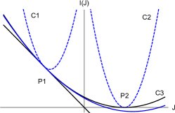
We remark that TUR (1) is equivalent to a geometric condition that the curve crosses the horizontal axis as a blue solid curve in Fig. 1. Actually, the nonnegativity of the discrimination of is nothing but (1).
Suppose TUR does not hold and the discrimination of is negative.
The conditions (5), (6), and the regularity condition imply that the curve corresponding to the actual rate function is tangent to the line and the horizontal axis, and locally follows the curves and with a common curvature at the points and .
Such a curve , however, is not convex and contradicts to the convexity of the rate function[40]. This completes the derivation.
Here, we compare our result with related works.
If the equality condition is fulfilled in TUR (1) then the curves and coincide and form a common global curve , which is essentially equivalent to the quadratic bound used for a class of stochastic processes[23, 24, 28].
If the discrimination is zero, corresponding to the rate function is given by .
Note that our geometric argument can also make clear the mechanism of the violation of TUR for a class of irregular distributions generated from the minimal distribution that has the smallest variance for a fixed mean value and is given as a sum of delta functions as reported in Ref. [35]. In our case, the minimal distribution reads
| (7) |
with an arbitrary positive constant .
The corresponding curve has the largest curvature proportional to the inverse of the variance . Therefore, the curve follows only in a close vicinity of the mean value. As a consequence, the bound of TUR (1) is available only approximately with sufficiently small values of the affinity . Furthermore, we can construct a class of TUR violating probability distributions by generalizing (7) to continuous but finite supports. Such distributions are expressed as
| (8) |
where is an even function as in Ref. [35] and importantly does not rapidly decay.
For instance, it is easy to numerically verify that the choices with also provide distributions which slightly violates the bound (1) for large [40] for the same reason as that of , i.e., the smallness of variance due to the non-sufficient decay of .
In contrast to the minimal distribution, the distributions for these choices of are continuous.
However, the support is exactly finite, which restricts the range of the fluctuation and is in marked contrast to the usual distributions of charge transfers with exponential tails.
Hence, (8) with the abovementioned choice of is regarded as the onset of the regularity condition.
Short time regime.— In the remaining of the Letter, to investigate further universal model-independent properties, we will consider the short time limit.
TUR applied to the short time limit claims that for the statistics of current, the mean and the variance satisfy the following theorem.
Theorem(Equality in a short time limit)
In a proper short time limit , the ratio of the thermodynamic precision and the half of the entropy production approaches unity
| (9) |
The use of the short time limit is certainly a limiting and strong condition[26, 35], however, we can apply (9) to the analysis of the universal relation among the scaling exponents for the charge transfer.
As a nontrivial consequence of (9), we will show the following corollary later in (18).
Corollary(Scaling of mean and variance in short time limit)
Let us independently vary the duration and the affinity [39].
If the mean of the charge transfer follows the scaling relation in the short time regime, i.e., and ,
| (10) |
as then the variance scales as
| (11) |
and vice versa.
Note that in the short time regime, the affinity is not necessarily small. As for the dependence, the validity of this corollary was experimentally verified for the electron current in a quantum dot[41] in the context of the full counting statistics.
Derivation of the relation among the scaling exponents.— The central limit theorem states that for sufficiently large the probability distribution obeys a normal distribution as
| (12) |
for
| (13) |
with a normalization constant and an dimensionless parameter [42]. Fix large but finite, the range of applicability (13) contains as the central region with a nonnegligible probability by taking sufficiently short so that is kept finite.
Then, a particular choice with fulfills the condition (13) in a proper short time regime. For this , we obtain
| (14) |
from (12). The main idea is to compare (14) with EFT applied to the probability distribution of the net charge transfer
| (15) |
To explain the validity of this scenario, let us investigate the asymptotic scaling behaviors of the mean and variance by assuming the following ansatz in the short time limit
| (16) |
and
| (17) |
where the coefficients , and standard values of the time scale and the affinity are constant. At the moment, the relation among the exponents , , , and are unknown.
The condition for the central limit theorem (13) requires that holds. By substituting (16) and (17) into this condition, a straightforward calculation shows that the choice
| (18) |
is a unique solution that satisfies (14), EFT (15), and (13). Interestingly, in the linear response regime, i.e., , becomes vanishingly small. We verified (18) in concrete examples in Supplemental Material.
Combining EFT (15) and (14), we can show that the fluctuation of the heat current satisfies
| (19) |
By multiplying the mean value , and using , equality of TUR (9) holds in the short time limit.
Similarly, we can obtain TUR equality in the short time limit for the external work.
Next, we will show a concrete example of TUR (1) and the equality (9) for Hamiltonian dynamics, which supports our perspective.
Example.—
We consider a one-dimensional oscillator with a time-dependent frequency as one of the simplest models with non-Gaussian probability distributions under the time symmetric driving protocol.
We explore the work done during as a charge transfer.
Let and denote the position and momentum of a particle with a mass , and let
| (20) |
denote the Hamiltonian at time . For concreteness, the time dependence of the frequency is assumed to be time symmetric under the protocol for and for with a natural frequency . Initially, the state is sampled from the canonical ensemble at a room temperature .
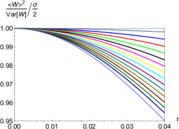
Then, we can explicitly solve the equation of motion, and calculate the work . We illustrate the TUR ratio as a function of in Fig. 2, and confirm TUR and (9). Since we are interested in mesoscopic systems, we fix the mass to and change the spring constant so that the period of oscillation is in the range between to . As shown in Fig. 3, the work distribution has a sharp peak, however, the TUR ratio actually converges to unity in the short time regime, which is in agreement with (19). We can also verify that (10) and (11) holds with the common exponent and by replacing and with and , respectively[40].

Conclusion.— We derived TUR for the charge transfer by a geometric argument on the rate function in terms of EFT and the central limit theorem applied to the ensemble of independent copies of the original system. In particular, TUR has a simple geometric interpretation in terms of the discrimination of the curve , which locally characterizes the statistics of rare events. In this manner, we directly revealed a link between important rigorous theorems TUR and EFT under a physical requirement of the regularity condition, which complements the insights gained in Refs. [26, 36, 35]. Exclusion of irregular distributions generated by the minimal distribution has a drawback that restricts the availability of our result, however, has also an advantage that no modification is necessary to the standard entropic bound. Hence, our result guarantees that TUR (1) holds for a large class of practical dynamics starting from a local Gibbs ensemble[13].
In the short time regime, TUR equality (9) holds beyond the linear response regime by fixing the affinity large but finite. If the net charge transfer quickly converges to the normal distribution[44, 43], the TUR equality (9) would accurately hold without taking the limit .
As a nontrivial corollary, we have shown a universal relation among the scaling exponents of the mean and variance of the charge transfer in the short time regime. This prediction is practically important e.g. for the electron transports in nanojunctions[41], for our example and for a stochastic description of a dragged colloidal particle in water[18]. The corollary provides a unified theoretical explanation for these observations.
Acknowledgements.
This work was supported by the Grant-in-Aid for Scientific Research (C) (No. 18K03467 and No. 22K03456) from the Japan Society for the Promotion of Science (JSPS).References
- [1] F. Hartmann, P. Pfeffer, S. Hofling, M. Kamp, and L. Worschech, Phys. Rev. Lett. 114, 146805 (2015)
- [2] K. Chida, S. Desai, K. Nishiguchi, and A. Fujiwara, Nat. Commun. 8, 15310 (2017)
- [3] K. Sekimoto, Prog. Theor. Phys. Suppl. 130, 17(1998)
- [4] U. Seifert, Phys. Rev. Lett. 95, 040602 (2005)
- [5] U. Seifert, Rep. Prog. Phys. 75, 126001 (2012)
- [6] D. J. Evans, E. G. D. Cohen, and G. P. Morriss, Phys. Rev. Lett. 71, 2401 (1993)
- [7] G. Gallavotti, and E. G. D. Cohen, Phys. Rev. Lett. 74, 2694 (1995)
- [8] J. Kurchan, J. Phys. A 31, 3719 (1998)
- [9] J. L. Lebowtiz, and H. Spohn, J. Stat. Phys. 95, 333 (1999)
- [10] G. E. Crooks, Phys. Rev. E 60, 2721 (1999)
- [11] C. Jarzynski, J. Stat. Phys. 98, 77-102 (2000)
- [12] P. Gaspard, J. Chem. Phys. 120, 8898 (2004)
- [13] C. Jarzynski and D. K. Wojcik, Phys. Rev. Lett. 92, 230602 (2004)
- [14] D. Andrieux and P. Gaspard, J. Chem. Phys. 121, 6167-6174 (2004)
- [15] D. Andrieux, P. Gaspard, T. Monnai, and S. Tasaki, New J. Phys. 11, 043014 (2009)
- [16] R. Rao, and M. Esposito, J. Chem. Phys. 149, 245101 (2018)
- [17] M. Esposito, U. Harbola, and S. Mukamel, Rev. Mod. Phys. 81, 1665 (2009)
- [18] G. M. Wang, E. M. Sevick, E. Mittag, D. J. Searles, and D. J. Evans, Phys. Rev. Lett. 89, 050601 (2002)
- [19] Y. Utsumi and K. Saito, Phys. Rev. B 79, 235311 (2009)
- [20] S. Nakamura, Y. Yamauchi, M. Hashisaka, K. Chida, K. Kobayashi, T. Ono, R. Leturcq, K. Ensslin, K. Saito, Y. Utsumi, and A. C. Gossard, Phys. Rev. Lett. 104, 080602 (2010)
- [21] K. Saito and Abhishek Dhar Phys. Rev. Lett. 99, 180601 (2007)
- [22] A. C. Barato and U. Seifert, Phys. Rev. Lett. 114, 158101 (2015)
- [23] T. R. Gingrich, J. M. Horowitz, N. Perunov, and J. L. England, Phys. Rev. Lett. 116, 120601 (2016)
- [24] T. R. Gingrich, G. M. Rotskoff, and J. M. Horowitz, J. Phys. A: Math. Gen. 50, 184004 (2017)
- [25] M. Polettini, A. Lazarescu, and M. Esposito, Phys. Rev. E 94 052104 (2016)
- [26] P. Pietzonka, A. C. Barato, and U. Seifert, Phys. Rev. E 93 052145 (2016)
- [27] P. Pietzonka, A. C. Barato, and U. Seifert, J. Stat. Mech. 124004 (2016)
- [28] J. M. Horowitz and T. R. Gingrich, Phys. Rev. E 96, 020103(R) (2017)
- [29] P. Pietzonka, F. Ritort, and U. Seifert, Phys. Rev. E 96, 012101 (2017)
- [30] J. M. Horowitz, and T. R. Gingrich, Nat. Phys. 16 15 (2020)
- [31] G. Guarnieri, G. T. Landi, S. R. Clark, and J. Goold, Phys. Rev. Research 1, 033021 (2019)
- [32] Y. Hasegawa, Phys. Rev. Lett., 125, 050601 (2020)
- [33] H. M. Friedman, B. K. Agarwalla, O. Shein-Lumbroso, O. Tal, and D. Segal, Phys. Rev. B 101, 195423 (2020)
- [34] T. Monnai, Phys. Rev. E 105, 034115 (2022)
- [35] A. M. Timpanaro, G. Guarnieri, J. Goold, and G. T. Landi, Phys. Rev. Lett. 123, 090604 (2019)
- [36] Y. Hasegawa and T. Van Vu, Phys. Rev. Lett. 123, 110602 (2019)
- [37] W. Feller, An Introduction to Probability Theory and Its Applications. Vol. 2nd ed, John Wiley & Sons, Inc. (1971)
- [38] R. S. Ellis, Entropy, Large Deviations, and Statistical Mechanics, Springer (1985)
- [39] Note that it is practical to regard and as independent variables by fixing the affinity and changing .
- [40] See Supplemental Material for more details of the regularity condition, the convexity of , and verifications of the scaling relations of and .
- [41] S. Gustavsson, R. Leturcq, T. Ihn, K. Ensslin, M. Reinwald, and W. Wegscheider, Phys. Rev. B 75, 075314 (2007)
- [42] Eq. (12) is a stronger statement than the stochastic convergence of the probability distribution , and is valid near the mean value .
- [43] H. B. Callen, An Introduction to Probability Theory and Its Applications. Vol. 1, 2nd ed, John Wiley & Sons, Inc. (1985)
- [44] In many cases, the convergence to the normal distribution in the central limit theorem is sufficiently rapid. The distribution function in Fig. 3 is an example.